Oriented ice eddy detection network based on the Sentinel-1 dual-polarization data

The complex convergence of cold and warm ocean currents in the Nordic Seas provides suitable conditions for the formation and development of eddies. In the Marginal Ice Zones (MIZs), ice eddies contribute to the accelerated melting of surface sea ice by facilitating vertical heat transfer, which influences the evolution of the marginal ice zone and plays an indirect role in regulating global climate. In this paper, we employed high-resolution synthetic aperture radar (SAR) satellite imagery and proposed an oriented ice eddy detection network (OIEDNet) framework to conduct automated detection and spatiotemporal analysis of ice eddies in the Nordic Seas. Firstly, a high-quality RGB false-color imaging method was developed based on Sentinel-1 dual-polarization (HH+HV) Extra-Wide Swath (EW) mode products, effectively integrating denoising algorithms and image processing techniques. Secondly, an automatic ice eddy detection method based on oriented bounding boxes (OBB) was constructed to identify the ice eddy and output features such as horizontal scales, eddy centers and rotation angles. Finally, the characteristics of the detected ice eddies in the Nordic Seas during 2022-2023 were systematically analyzed. The results demonstrate that the proposed OIEDNet exhibits significant performance in ice eddy detection.

1 Introduction

Ocean eddies are a pervasive oceanic phenomenon that plays a significant role in the transport and distribution of material, energy, heat, and freshwater in the global ocean (Chelton et al., 2011; Zhang et al., 2020). The observational advantages of SAR satellites, which operate in all weather conditions and at all times of the day, and offer high spatial resolution, make them an important data source for the refined study of oceanic eddies. SAR satellites are essential for the study of submesoscale eddies that remain unobservable by altimeter satellites. The remote sensing imaging mechanism of SAR ocean eddies is mainly influenced by two mechanisms (ZHENG et al., 2018; Fu and Holt, 1983; Karimova et al., 2012): the wave-current interaction mechanism and the sea surface floating tracer mechanism, such as bio-oil films and ice floes. In the MIZs, surface sea ice is driven by ocean eddies, exhibiting spiral motion and eddy characteristics (Manucharyan and Thompson, 2017). This paper refers to the ice-water mixing pattern formed by surface sea ice and ocean eddies as an ice eddy (Johannessen et al., 1987; Dumont et al., 2011). The melting of surface ice is facilitated by ice eddies through the vertical transfer of heat, which affects the development of MIZs and indirectly influences global climate regulation.

Data acquisition for ice eddies relies on both in situ instruments and satellite sensors. In general, in situ observations are characterized by their high quality and reliability and include moorings (Cassianides et al., 2021; von Appen et al., 2018), ice-tethered profilers (Toole et al., 2011), and under-ice gliders. However, due to the high cost of observations and poor weather conditions, the amount and coverage of in situ observational data may not adequately support experimental demands. Satellite sensors theoretically possess the capability to acquire vast amounts of data, supporting ice eddy detection and characterization tasks with high spatial resolution and wide-area global observation. In the Arctic Ocean, the detection of submesoscale and small-scale eddies using satellite altimetry data is challenging due to the limited spatial and temporal coverage of both altimetry and in situ data. The Rossby radius of deformation in the Arctic Ocean is significantly smaller than in mid- and low-latitude seas (Bashmachnikov et al., 2020; Nurser and Bacon, 2013). Due to the presence of sea ice, the complexity of using altimeter data in the Arctic Ocean renders it nearly unsuitable for detecting ice eddies. Observational costs and adverse weather limit the quantity and coverage of in situ data, which may be insufficient to meet experimental demands. In contrast, SAR satellites with high spatial resolution, full-time, and all-weather capability are better suited for detecting mesoscale and submesoscale oceanic phenomena in the Arctic Ocean (Kozlov et al., 2019). SAR satellites have become essential in in-depth studies of oceanic eddies, particularly submesoscale eddies challenging to detect with altimeter satellites. The unique advantages of SAR satellites are illustrated in Figure 1.

Figure 1

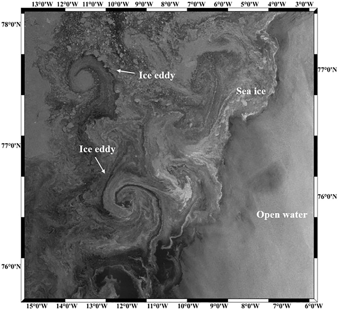
Figure 1. S1 EW HH-polarized SAR image, 6 August 2022,07:47 UTC.

The detection of eddies using SAR imagery has been the focus of numerous studies (Cassianides et al., 2021; Kozlov and Atadzhanova, 2021; Manucharyan and Thompson, 2017). However, most studies rely on manual visual interpretation methods for the detection of eddies from SAR images (Toole et al., 2011; Gupta and Thompson, 2022). The accumulation of massive SAR images has rendered it time-consuming and laborious to recognize ocean eddies solely through manual visual interpretation, highlighting the growing importance of automated ocean eddy detection. In recent years, several researchers have applied deep learning methods to ocean eddy detection on synthetic aperture radar (SAR) images (Zhang et al., 2023; Xia et al., 2022; Huang et al., 2017; Du et al., 2019b; Zhang et al., 2020). Du et al. (2019a) attempted to fuse a variety of features to automatically identify ocean eddies and proposed an eddy identification method based on adaptive weighted multi-feature fusion for SAR images. Considering the different importance of different features for eddy recognition, an adaptive weighted feature fusion method based on multiple kernel learning (MKL) is also proposed. Although MKL demonstrates excellent performance in addressing heterogeneous data, the method exhibits low detection efficiency. Du et al. (2019b) proposed DeepEddy, a deep learning-based ocean eddy detection method consisting of a hierarchical feature learning model and a simple Support Vector Machine (SVM) classifier. Eddy features are learned using two principal component analysis convolutional layers. Additionally, DeepEddy employs Spatial Pyramid Pooling (SPP), which addresses the complex structure and morphology of ocean eddies by fusing multi-scale features. However, this method fails to localize eddies on SAR images. Zhang et al. (2023) proposed EddyDet, a deep framework based on the Mask RCNN framework utilizing Convolutional Neural Networks for eddy detection on SAR images. Khachatrian et al. (2023) applied the YOLOv5 network to SAR ocean eddy detection and realized the automatic detection of ice eddies in the MIZs. Zi et al. (2024) proposed an EOLO network to enhance the feature fusion method by introducing a channel attention mechanism and employing an upsampling operator with a larger receptive field. Xia et al. (2022) constructed a context and edge association network (CEA-Net) based on the YOLOv3 backbone network for identifying ocean eddies in S1 interferometric wide (IW) swath mode data. While the automatic detection of eddies in SAR images using deep learning has shown promising results, current research emphasizes the detection of eddies in ice-free areas within mid- and low-latitude waters through the use of co-polarization SAR images. HH-polarized images make small-scale features more visible, while HV-polarization provided more stable large-scale features related to sea-ice morphology (Korosov and Rampal, 2017). The HV-polarized images were less sensitive to surface scattering from open water but were very sensitive to body scattering from sea ice. As a result, the contrast between sea ice and open water is higher in HV-polarized images, making ice eddy features more visible (Qiu and Li, 2022). The advantages of HH-polarized images in detecting ice eddies are due to its high sensitivity to surface scattering, its strong contrast with open water, and its high signal-to-noise ratio, particularly under low wind speed or rough surface conditions, where HH polarization can offer precise and reliable ice eddy detection results. Combining HH-polarization and HV-polarization features for ice eddy detection, compared to using a single polarization, is beneficial for reducing detection errors and improving accuracy.

Although the aforementioned methods have achieved superior results in eddy detection in SAR images, they all utilize the conventional horizontal bounding box (HBB) and still exhibit notable limitations. HBBs are not optimal for representing oceanic ice eddies with arbitrary orientations and large aspect ratios, as they provide only a rough location without accurate directional and scale information. Additionally, the HBB representation often includes excessive background or nearby object interference, which can lead to misidentification of ice eddies. Unlike HBBs, OBBs are capable of flexibly adjusting the orientation of detection boxes, allowing for the accurate enclosure of inclined or rotated ice eddies. This capability addresses issues related to redundant and overlapping detection boxes, thereby significantly reducing detection errors. The field of target detection has made remarkable progress over the past decade. Directional target detection, as an extended branch of target detection, has attracted significant attention due to its wide range of applications (Li et al., 2020; Liu et al., 2020; Han et al., 2021; Xia et al., 2018; Ma et al., 2018; Ding et al., 2019; Yang et al., 2019). Ice eddies have distinct rotational characteristics and directionality, and directional target detection can not only detect the position of eddies but also accurately estimate their rotational direction, which is highly significant for ocean dynamics research, marine environment monitoring, and marine resource development.

To address the above challenge, in this paper, we proposed OIEDNet, which is a oriented ice eddy detection network based on the Sentinel-1 dual-polarization data. The remainder of this paper is structured as follows. Section 2 provides an overview of the dataset. Section 3 describes the methodology employed in this study. Section 4 presents the experimental results and discussion. Finally, conclusions are outlined in Section 5.

2 Materials

We utilize Sentinel-1A Level-1 EW mode Ground Range Detected (GRD) product. The swath width for the EW Mode is approximately 400 km, with an incidence angle ranging from 18.9° to 47° and a pixel spacing of 40 m × 40 m. We selected 702 Sentinel-1 SAR images containing ice eddies in the marginal ice area of the Nordic Seas during January 2022-December 2023 as shown in Table 1 and Figure 2.

Table 1

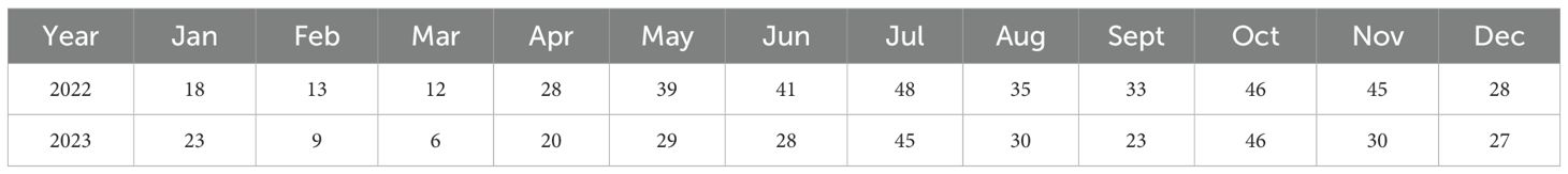
Table 1. SAR data statistics for Nordic ice eddy detection (S1).

Figure 2

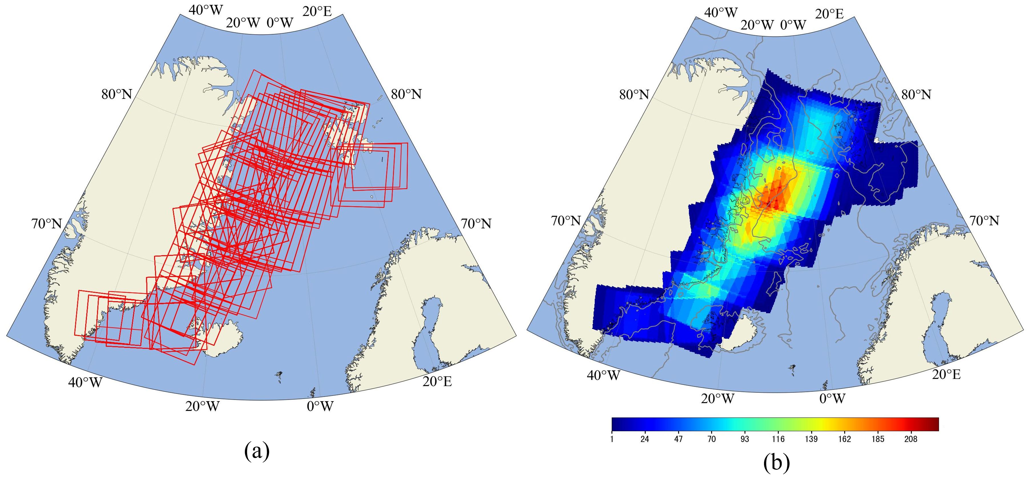
Figure 2. The distribution of experimental SAR images collected in the marginal ice zone of the Nordic Seas from January 2022 to December 2023. (A) Spatial coverage of SAR images. (B) The number of SAR images is represented by color intensity. The gray lines indicate the 200 m and 2000 m isobaths, derived from IBCAOv4.0.

The bathymetric product is the 200m resolution version 4.0 of the International Bathymetric Chart of the Arctic Ocean (IBCAOv4.0) (Jakobsson et al., 2020). The relationship between the intensity of ice eddy production and the background wind velocity was analyzed using 10m u and v hourly means from the ERA-Interim reanalysis. The validation was conducted using the Level 3 (L3) products from the Surface Water and Ocean Topography (SWOT) mission, the Mesoscale Eddy Trajectory Atlas Product (META3.1exp DT), the situ data collected from OpenMetBuoys-v2021 (OMBs) deployed in the marginal ice zone (Rabault et al., 2024) and drifters 15m drogue.

3 Methods

The pipeline of the proposed OIEDNet framework is depicted in Figure 3. From this figure, it is evident that the proposed framework consists of three components: the Polarization Combination Enhancement Module, the Neural Network Module, and the Feature Statistical Analysis Module.

Figure 3

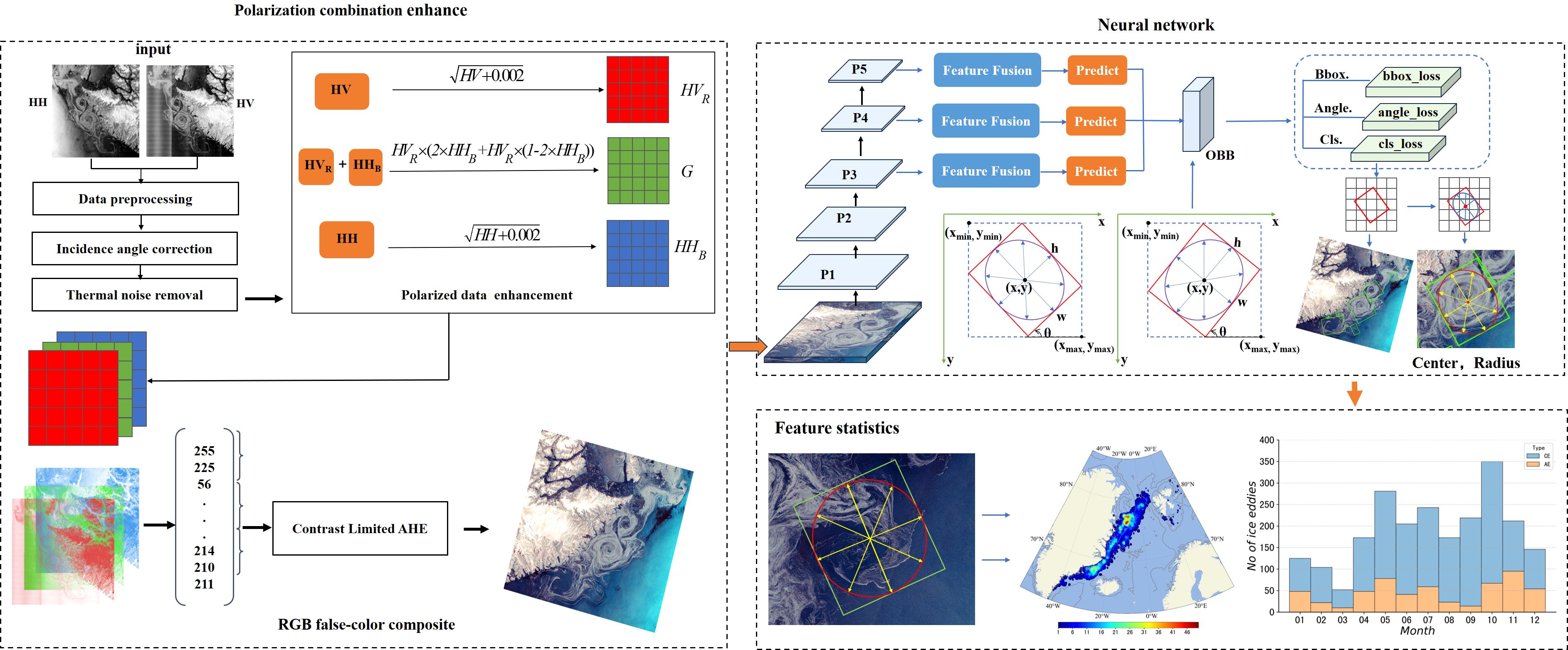
Figure 3. The structure of the proposed OIEDNet framework.

Firstly, the Sentinel-1 satellite’s HH and HV dual-polarized ice eddy SAR images undergo data preprocessing, HH-polarized incidence angle correction (IAC), HV-polarized thermal noise removal (TNR), and dual-polarized false-color image synthesis to generate dual-polarized SAR false-color ice eddy images. Secondly, the ice eddy sample library is created using the data expansion method. Finally, based on the dual-polarized SAR false-color ice eddy images, a rotating frame ice eddy auto-detection model is developed and trained to achieve the automatic detection of ice eddies in the Nordic Seas MIZs.

3.1 Polarization combination enhancement method

The polarization combination enhancement method includes (1) data preprocessing; (2) HH-polarized IAC; (3) HV-polarized TNR; (4) polarized data enhancement, and (5) RGB false-color composite. Figure 4 illustrates the flowchart of the polarization combination enhancement process. Data preprocessing mainly involves orbit correction, radiometric calibration, filtering, conversion to dB values, and geocoding processing.

Figure 4

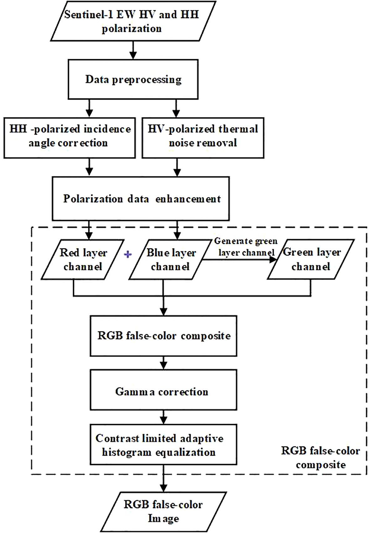
Figure 4. Flowchart of the polarization combination enhancement method.

In the process of ice eddy detection, the variation in the backward scattering coefficient caused by changes in the incidence angle may introduce significant errors, necessitating the correction of the incidence angle for HH-polarized data. In this study, the IAC algorithm (Qiu and Li, 2022; Li et al., 2020) is utilized, and the calculation formula is presented in Equation 1.

$\begin{array}{ll}\sigma ={\sigma }^0+0.200\times (\theta -{\theta }_0),& (1)\end{array}$

where σ is the corrected backward scattering coefficient (in dB), ${\sigma }^0$ is the backward scattering coefficient before correction, θ is the incidence angle of the pixel, and ${\theta }_0$ is the corrected standard incidence angle, which is taken as 34.5°. Figure 5D illustrates the effects following the correction of the HH polarization incidence angle.

Figure 5

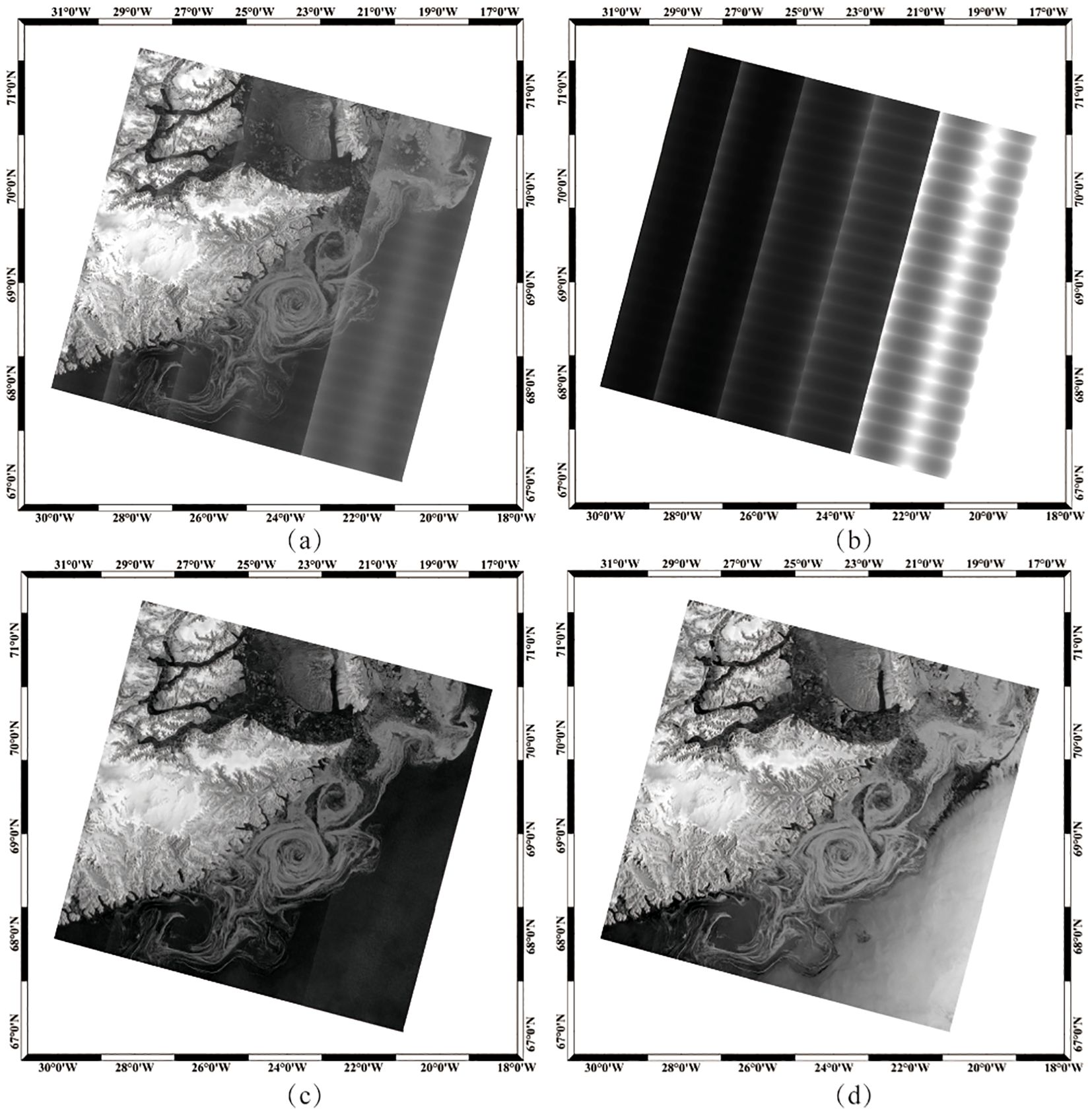
Figure 5. Effect of HV TNR and HH IAC. (A) Original HV polarized image. (B)The thermal noise in HV polarized images. (C) HV polarized image after TNR, (D) HH polarized image after IAC (S1 EW image taken on 1 November 2023 at 08:21:44 UTC).

In Sentinel-1 EW-mode SAR images that are strongly affected by scallop stripe noise in the azimuth direction and by noise gradients in the distance direction, especially in HV-polarized images, thermal noise is particularly prominent as displayed in Figures 5A, B. Although ESA provides a standard method of noise vector correction, the effect of residual noise cannot be ignored due to the narrow distribution of HV polarization backscatter.

The denoising algorithm (Park et al., 2017; Sun and Li, 2020) was improved for the removal of thermal noise. The average noise power was added to the denoised results. This adjustment enabled the conversion of noise power from a linear scale to a logarithmic scale (dB) sigma zero conversion, ensuring that these pixels did not become invalid values. By appropriately scaling and balancing the noise vectors given by ESA, the algorithm can approximate the actual noise values as much as possible by using the azimuthal antenna element pattern in the azimuthal direction, so that the effects of the scallop stripe and the noise gradient in the distance direction can be effectively eliminated. The specific processing steps are as follows.

To eliminate the noise step phenomenon between sub-bands, it can be assumed that the denoising process model satisfies a linear relationship. It is calculated using Equation 2.

$\begin{array}{ll}s(k)={\sigma }_{SN}^0-(K_{ns,n}·G•{\sigma }_N^0+K_{pb,n}^0),& (2)\end{array}$

where $s(k)$ is the denoised ${\sigma }^0$ value. ${\sigma }_{SN}^0$ is the uncorrected original ${\sigma }^0$ value. ${\sigma }_N^0$ is the ${\sigma }^0$ calculated by bilinear interpolation using the thermal noise vector provided by ESA. $K_{ns,n}$ is the optimal noise scaling factor. $K_{pb,n}^0$ is the interstrip noise power balance factor. n is the number of sub-bands, n = 1, 2, 3, 4, 5. $K_{ns,n}$ can be obtained by least squares solution using a large amount of HV polarized data. $K_{pb,n}^0$ can be calculated using Equation 3.

$\begin{array}{ll}{K}_{pb,n}^0=({\alpha }_{n-1}i+{\beta }_{n-1})-({\alpha }_{n}i+{\beta }_n),& (3)\end{array}$

where ${\alpha }_n$ and ${\beta }_n$ are the slopes and intercepts, respectively, of the linear models for the different sub-strips. i is the number of image elements in the range direction at the boundary between the strips n = 2, 3, 4, 5. Since there are only four interstrip boundaries. $K_{pb,1}^0$ is set to 0.

When the original image is subtracted from the thermal noise acquired using the described method, some image element points become negative. To eliminate the effect of negative noise power, noise compensation is required. By appropriately scaling and balancing the noise vectors provided by ESA, the algorithm can closely approximate the actual noise values using the azimuthal antenna element pattern, effectively eliminating the effects of scallop stripes and noise gradients in the range direction.

First, the Signal-Noise Ratio (SNR) is defined as the ratio of the ${\sigma }^0$ value $(s_{0g})$ after Gaussian filtering to the noise equivalent sigma zero (NESZ). The SNR is calculated using Equation 4.

$\begin{array}{ll}\text{SNR}=\frac{s_{0g}}{\text{NESZ}}.& (4)\end{array}$

Subsequently, further calculations were conducted to obtain the power compensated using Equation 5.

$\begin{array}{ll}{s}_{0o}=\frac{\text{weight }\times s_{0g}+ \text{SNR }\times s_0}{\text{weight }+\text{ SNR}}+s_{0\text{offset}},& (5)\end{array}$

where $s_{0o}$ is the residual noise power compensated ${\sigma }^0$. $s_{0\text{offset}}$ is the noise field compensation value, which can be taken as the average value of the reconstructed noise field.

Finally, the HV polarization grayscale image with thermal noise removed can be obtained. Figure 5C illustrates the effects after the removal of thermal noise from the HV polarization.

In this paper, a high-quality dual-polarization SAR RGB false-color ice eddy image production method is proposed, compositing HH and HV polarizations into a single false-color image. Since the ice eddy information in the Sentinel-1 EW model is primarily contained in the HH-polarized data, the HH-polarized image is used for the blue channel and the HV-polarized image for the red channel. To optimize the visual quality, the square root is applied to the HH and HV channels, with a slight offset added to mitigate the effect of grain noise on the data. The calculation formula is presented in Equation 6 and Equation 7.

$\begin{array}{ll}H{H}_B=\sqrt{HH+0.002}.& (6)\end{array}$

$\begin{array}{ll}H{V}_R=\sqrt{HV+0.002}.& (7)\end{array}$

The green channel image is produced by combining the offset-processed HH and HV polarization data, as shown Equation 8.

$\begin{array}{ll}G=H{V}_R\times (2\times H{H}_B+H{V}_R\times (1-2\times H{H}_B)).& (8)\end{array}$

Finally, the SAR image was enhanced using SAR image stretching and contrast-limited adaptive histogram equalization (CLAHE). Figure 6 illustrates a comparison the RGB false color images before and after denoising.

Figure 6

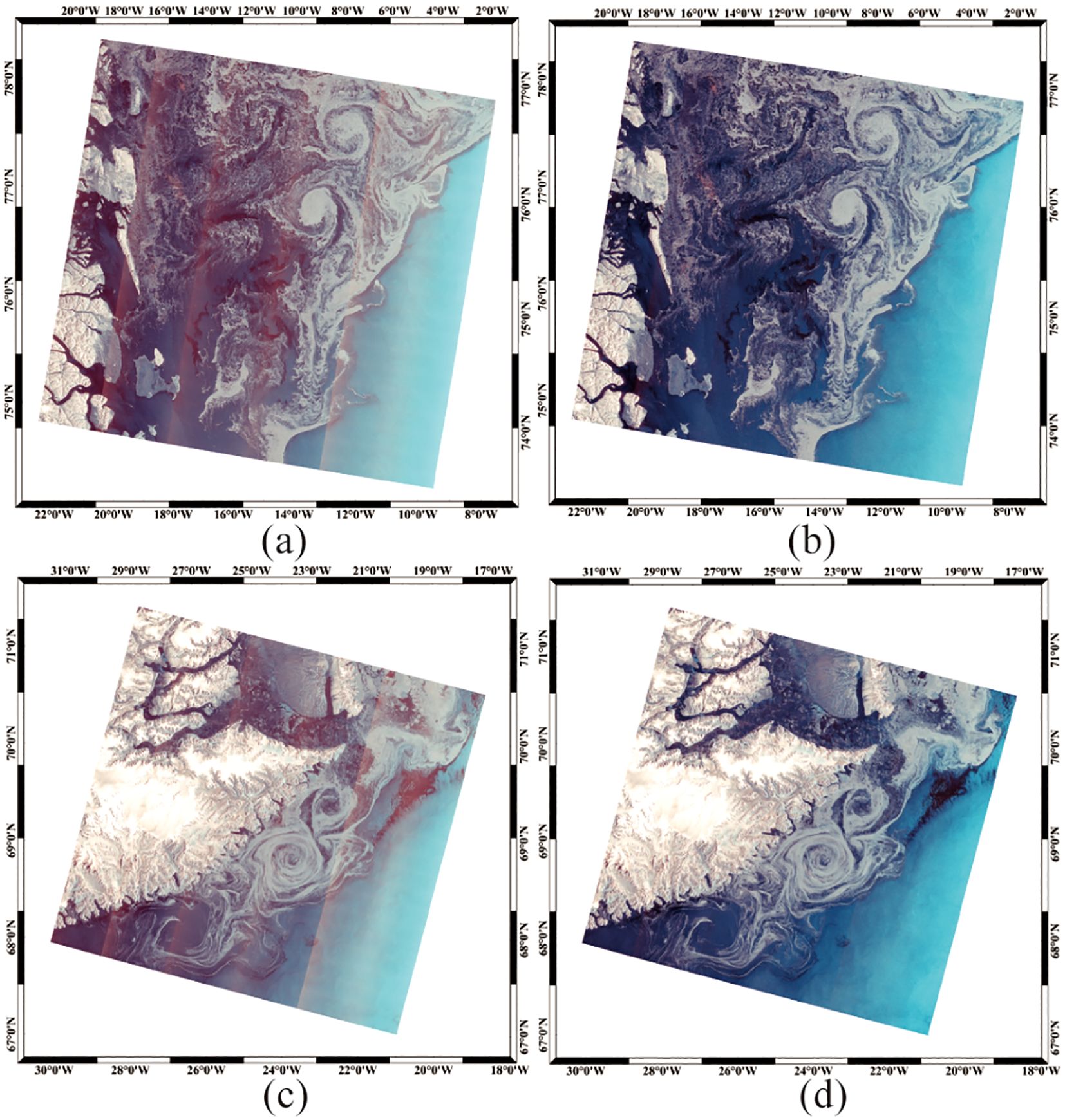
Figure 6. Comparison of the RGB false-color images before and after denoising. A comparison of the RGB false-color images before and after denoising is presented. (A, C) represent the RGB images prior to denoising, while (B, D) represent the RGB images following denoising. (A, B) correspond to the S1 EW image acquired on 28th September 2023 at 08:03:22 UTC, while Figures (C, D) correspond to the data acquired on 1st November 2023 at 08:21:44 UTC.

The data expansion of 702 dual-polarized false-color ice eddy images was achieved through noise perturbation transformations, rotations (90°, 180°, 270°), and up-down flip transformations, resulting in dual-polarized ice eddy samples. Eddies that rotate clockwise in the northern hemisphere are referred to as anticyclonic eddies, while those that rotate counterclockwise are referred to as cyclonic eddies. Figure 7 illustrates examples of anticyclonic and cyclonic ice eddies.

Figure 7

Figure 7. Examples of ice eddies photographed by S1. (A–C) are anticyclonic eddies and (D–F) are cyclonic eddies.

3.2 Neural network

In this paper, we propose the neural network component of OIEDNet, a multiscale rotating frame model designed for the automatic detection of ice eddies. The model structure is illustrated in Figure 8. Traditional target detection algorithms typically utilize HBB, assuming that object positions in the image are calculated relative to the image center. However, this assumption is not always accurate, particularly for objects with distinct directional features, as the HBB often fails to accurately locate the true position of such objects. OIEDNet addresses this limitation by introducing OBB, which allow bounding boxes to be positioned at any arbitrary angle, making it more adaptable for detecting target objects with various orientations.

Figure 8

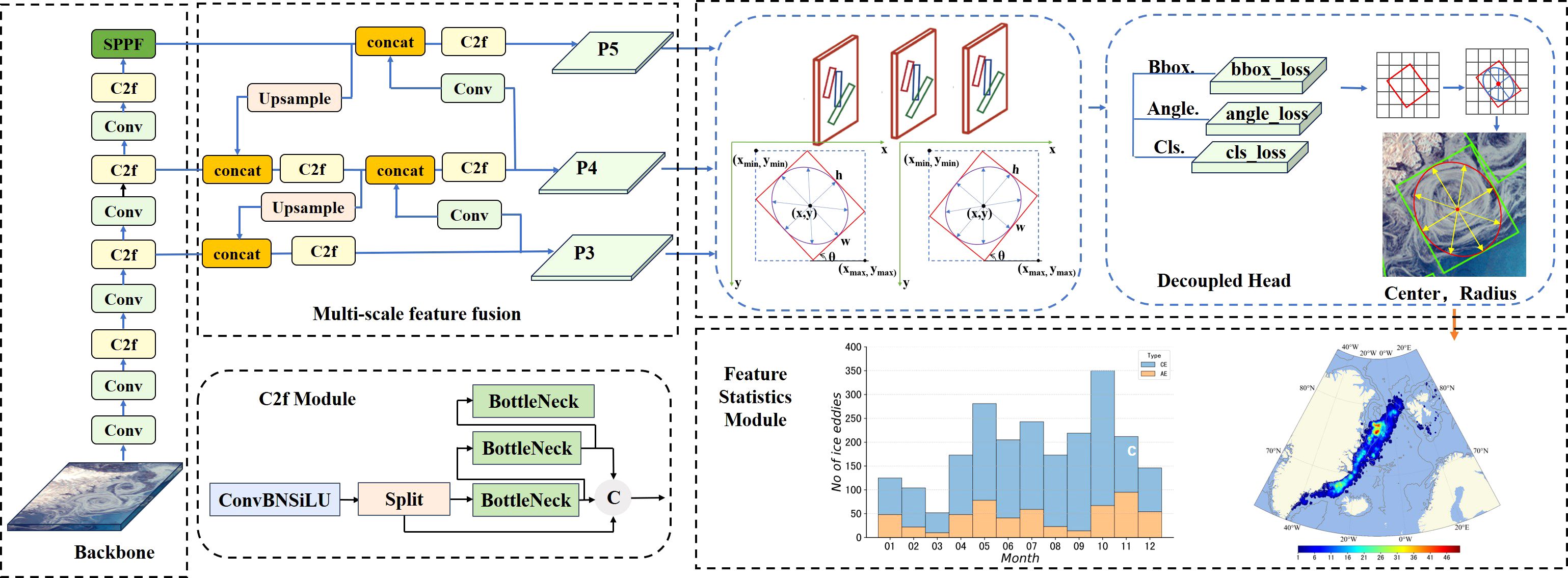
Figure 8. The detailed structure of the neural network part of OIEDNet.

3.2.1 Feature spatial pyramid module

The backbone of OIEDNet consists of the CSPDarknet53 feature extractor, which is followed by a C2f module. The C2f module is succeeded by two segmentation heads designed to predict the semantic segmentation masks of the input images. Submesoscale ice eddies (approximately 0.1 to 10 km) and mesoscale ice eddies (approximately 10 to 100 km) can be detected by SAR satellites. To address the wide range of ice eddy target scales in SAR images, a feature fusion module is integrated into CSPDarknet53 to fuse feature maps of varying scales, enhancing the detection of ice eddies of different sizes. OIEDNet incorporates the Spatial Pyramid Pooling Faster (SPPF) module in the feature-enhanced Neck layer, which is optimized from the original SPP module structure. To obtain high-level semantic information from multiscale features and further improve detection accuracy and speed, The SPPF module is inserted between the convolutional and fully connected layers. The SPPF module integrates multiscale local feature information, providing the network with a global perspective and facilitating the extraction of rich multiscale feature representations, as illustrated in Figure 9. The original SPP module generates a final feature map by connecting three feature maps processed in parallel with 5 × 5, 9 × 9, and 13 × 13 max pooling kernels. However, this approach is time-intensive. To improve operational efficiency and detection speed, the SPPF module optimizes this process by merging the feature map processed by a mixed layer (convolutional layer + BatchNorm layer + SiLU layer) with three feature maps derived from a single 5 × 5 max pooling operation. This concatenation enables efficient extraction of the final feature map.

Figure 9

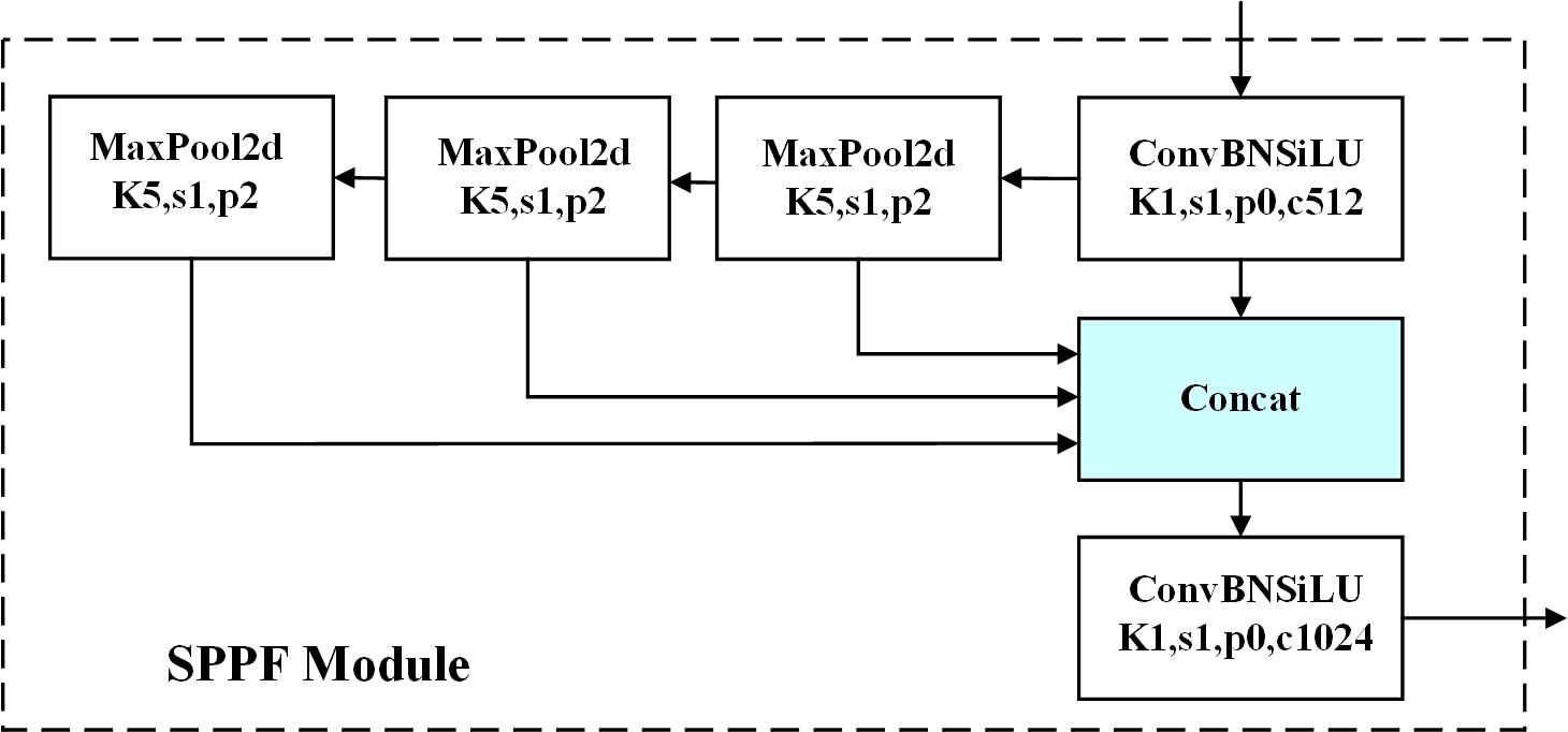
Figure 9. The structure of the Spatial Pyramid Pooling Faster module.

Traditional Feature Pyramid Networks (FPNs) enhance the representation of low-level features by transferring high-level features downwards through a top-down pathway (Lin et al., 2017). Nonetheless, traditional FPNs face challenges in effectively managing scale variations. To compensate for this deficiency, OIEDNet introduces the Progressive Asymmetric Feature Pyramid Network (PAFPN) structure (Liu et al., 2018), which enhances the performance of the target detection task by fusing features from neighboring levels and incorporating higher-level features into the fusion process in an incremental manner, enabling direct interaction between non-neighboring levels. PAFPN is applied between a feature extraction network (backbone) and a neck network (neck module). Specifically, different levels of feature maps are first extracted by the backbone, and then feature fusion is performed using PAFPN. The fused feature maps are fed into OIEDNet’s head network (head module) for object classification and bounding box regression. PAFPN incorporates the Path Aggregation Network (PAN) into the Feature Pyramid Network (FPN) by employing a bottom-to-top fusion approach. OIEDNet replaces the Context Enhancement Module (C3) in PAN with a Context Enhancement Module with feature fusion (C2f) and removes the 1×1 convolution prior to upsampling. OIEDNet directly inputs the feature output from various stages of the backbone into the upsampling operation. The PAFPN network structure enables the construction of multi-scale feature maps from a single image, ensuring that each layer of the pyramid produces feature maps with robust semantic information. This approach provides richer spatial detail and high-level semantic features for detecting marine ice eddies, which exhibit complex structures, varying scales, and rapid, continuous changes.

3.2.2 Rotation bounding box

Five variables $(cx,cy,w,h,\theta )$ are used to define the bounding box with an arbitrary orientation. As shown in Figure 10, cx and cy represent the coordinates of the center point, and the rotation angle θ indicates the angle between the horizontal axis and the first edge of the rectangle after counterclockwise rotation. Here, the first edge defines the width of the bounding box, while the other edge defines its height, with the angle ranging from -90° to 0°.

Figure 10

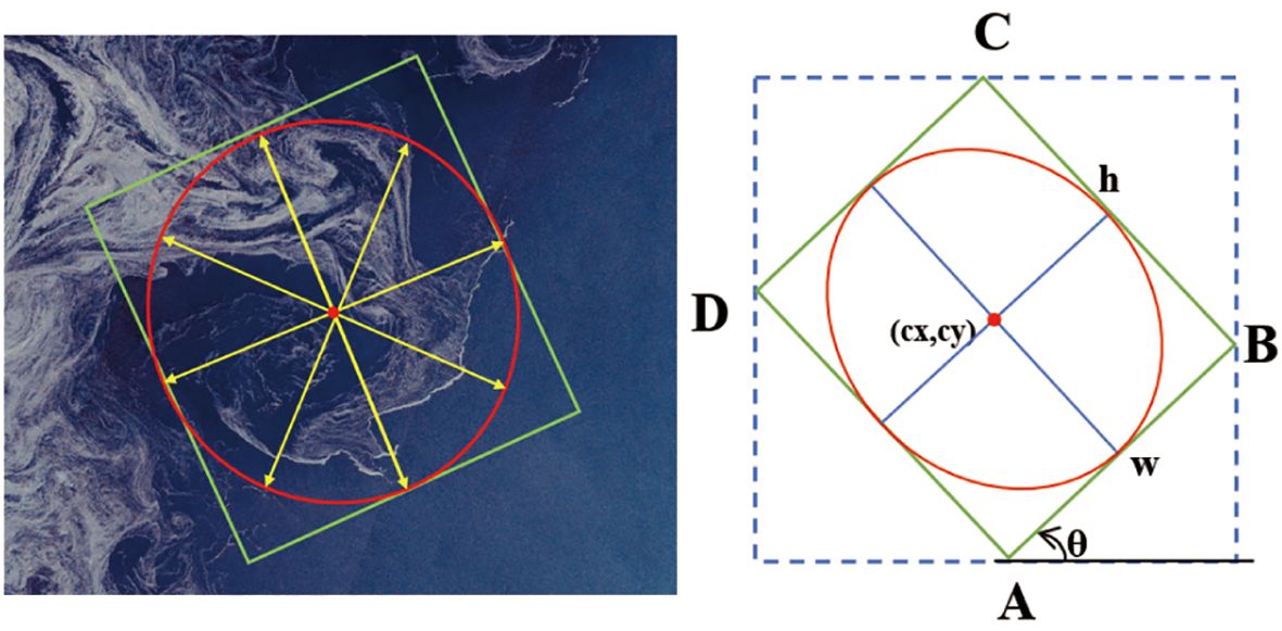
Figure 10. Oriented bounding boxes(green solid lines).The red ellipse represents the eddy edge, while yellow arrows show the distance from the eddy center to any point on the ellipse. A red dot marks the center of the ice eddy.

3.3 Feature statistical analysis module

Based on the obtained location information, the center and diameter of the ice eddy in the predicted box can be determined, laying the foundation for subsequent ice eddy studies. The center of the tangent ellipse inside the rotating frame was used as the eddy center, and the average distance from the center of the ice eddy to all points on the fitted ellipse is used as the radius of the ice eddy. According to the ice eddy automatic detection model, the rotating frame parameters $(cx,cy,w,h,\theta )$ of the ice eddy are obtained. Using the eddy center $(cx,cy)$ as the starting point, the coordinate positions of the four vertices A,B,C,D can be calculated.

During the data preprocessing stage, SAR images are geocoded using the WGS1984 standard, transforming pixel coordinates (rows and columns) into geographic coordinates (longitude and latitude). Consequently, it becomes possible to calculate the location of the ice eddy center and the eddy diameter. The Feature Statistical Analysis Module primarily facilitates the extraction of ice eddy center and diameter information, and performs statistical analyses to produce thematic maps of ice eddies for any time period and any region. These maps depict the spatial distribution of ice eddies and related scale histograms (see Chapter 4.4). These analyses support researchers in examining the generative mechanisms and evolutionary processes of ice eddies.

4 Experimental results and discussion

4.1 Experimental environment

The experimental setup configuration is provided in Table 2. Computation was performed on GPUs with 16 multithreads, and the training data share was configured to 0.75. The RGB ice eddy training set and S1 annotations were employed for training, and the model’s parameters were fine-tuned based on experience and experimental results to attain optimal performance.

Table 2

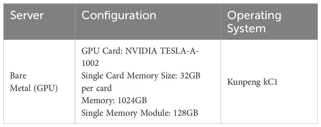
Table 2. Experimental setup configuration.

YOLOX is an open-source high-performance detector that builds upon YOLOv3 by introducing decoupled heads, data augmentation, anchor-free detection, and the SimOTA sample matching method, thus constructing an end-to-end anchor-free object detection framework (Zheng et al., 2021). YOLOv8 is a real-time object detection model that utilizes advanced techniques such as anchor-free detection and multi-scale feature fusion within a HBB framework (Varghese and Sambath, 2024). We conduct comparative experiments on OIEDNet, YOLOX and YOLOv8. In addition, we conduct multi-model comparison experiments to evaluate performance before and after denoising, and between single polarization and dual polarization.

The precision evaluation of the model is based on the validation set, and the evaluation metrics include the precision rate (P), the recall rate (R) and the F1-Score (F1), as shown in Equations 9–11.

$\begin{array}{ll}P=\frac{TP}{TP+FP}.& (9)\end{array}$

$\begin{array}{ll}R=\frac{TP}{TP+FN}.& (10)\end{array}$

$\begin{array}{ll}F1=2\times \frac{P\times R}{P+R}.& (11)\end{array}$

TP denotes the number of correctly detected ice eddies, FP denotes the number of false positive detections of ice eddies, and FN denotes the number of missed ice eddies.

4.2 Comparison

The results of OIEDNet,YOLOX and YOLOv8 were compared using the same test set, as presented in Table 3. Both YOLOv8 and YOLOX are traditional HBB detection models. The experimental results indicate that the OIEDNet model exhibits a precision of 94.40% and a recall of 93.65%, while YOLOv8 and YOLOX exhibit precisions of 93.50% and 87.90%, as well as recalls of 92.00% and 86.51%. In comparison to YOLOv8 and YOLOX, the OIEDNet model demonstrates superior performance in detecting dense eddy regions. The rotational detection of OIEDNet more accurately detects eddies with irregular shapes and changing directions, and the inspection frame fits the eddies more closely, significantly reducing the redundancy of the horizontal inspection frame, as shown in Figure 11. For eddies with large differences in scales and similar locations, there is obvious overlapping of inspection frames in horizontal detection, while rotational detection effectively avoids overlapping of inspection frames (Figure 11B). The interaction between ocean circulation and ocean currents is accompanied by the splitting and fusion of ocean eddies, leading to the multinucleated structure of ice eddies, which the rotational detection method can detect more accurately (Figure 11D). The IEDNet model reduces the leakage and false alarms of ice eddies to a certain extent. The OIEDNet model has obvious advantages in the precision and recall of ice eddy detection, and it can effectively detect submesoscale and mesoscale ice eddies.

Table 3

Table 3. Accuracy evaluation of different models.

Figure 11

Figure 11. The comparison of ice eddy detection results between OIEDNet and YOLOv8 is shown in (A–D) where the red HBB is used to represent YOLOv8 detection results, and the green OBB is used to represent OIEDNet detection results.

This study evaluates the enhancement effects of IAC, TNR, and dual-polarization RGB false color synthesis in the OIEDNet model. Comparison of four sets of ice eddy detection results for the same OIEDNet model (Figure 12). Before and after the denoising of dual-polarized false-color images, the detection accuracy increases from 88.71% to 94.40%, reflecting an improvement of 5.69%. In contrast, the detection accuracy of ice eddies in HV-polarized images without TNR is 85.04%, while the detection accuracy in HH-polarized images without IAC is 89.06%. This indicates that thermal noise significantly reduces the detection accuracy of ice eddies, whereas the incidence angle has a relatively minor effect on detection accuracy. The detection performance of the proposed model shows significant improvement with the adoption of the Polarization Combination Enhancement, resulting in an approximate 8.65% increase in the F1 score. This enhancement effectively boosts detection accuracy in noise-heavy environments.

Figure 12

Figure 12. Comparison of four sets of ice eddy detection results using the OIEDNet model: (A) detection results without HH-polarized IAC, (B) detection results without HV-polarized thermal noise reduction, (C) detection results of dual-polarized RGB images before denoising, and (D) detection results of dual-polarized RGB images after denoising.

4.3 Validation

Altimeters and SWOT satellites rely on radar echo signals for measuring sea surface height. However, sea ice leads to attenuation and scattering of radar signals, rendering the echo signals unstable, which makes it difficult to obtain accurate sea surface height data and, therefore, makes it unable to accurately detect ice eddies, as shown in Figures 13, 14. SAR, on the other hand, can clearly detect ice eddies in this environment due to its high-resolution imaging and penetration capabilities. Mesoscale eddies can be identified from sea level height data using altimetry, but the daily mesoscale eddy dataset is identified by measuring different time trajectories, which results in low spatial and temporal resolution. Figures 13B, 14B shows a comparison of eddies identified by OIEDNet and altimeters. It is clear that SAR is able to detect more submesoscale ice eddies and that SAR is even more advantageous in detecting high-latitude ice eddies.

Figure 13

Figure 13. Comparison of the ice eddy identification results from OIEDNet (green) with those obtained from SWOT, drifting buoys(yellow), and the mesoscale eddy track atlas product META3.1exp DT (red). (A, B) data time are S1: 2023-10-15 08:13:37 UTC. SWOT: 2023-10-15 03:43:56 UTC, META3.1exp DT: 2023-10-15 UTC. drifting buoys(5801987): from 2023-10-1 to 2023-10-15 UTC. The orange arrow in (B) indicates the trajectory of the drifting buoy.

Figure 14

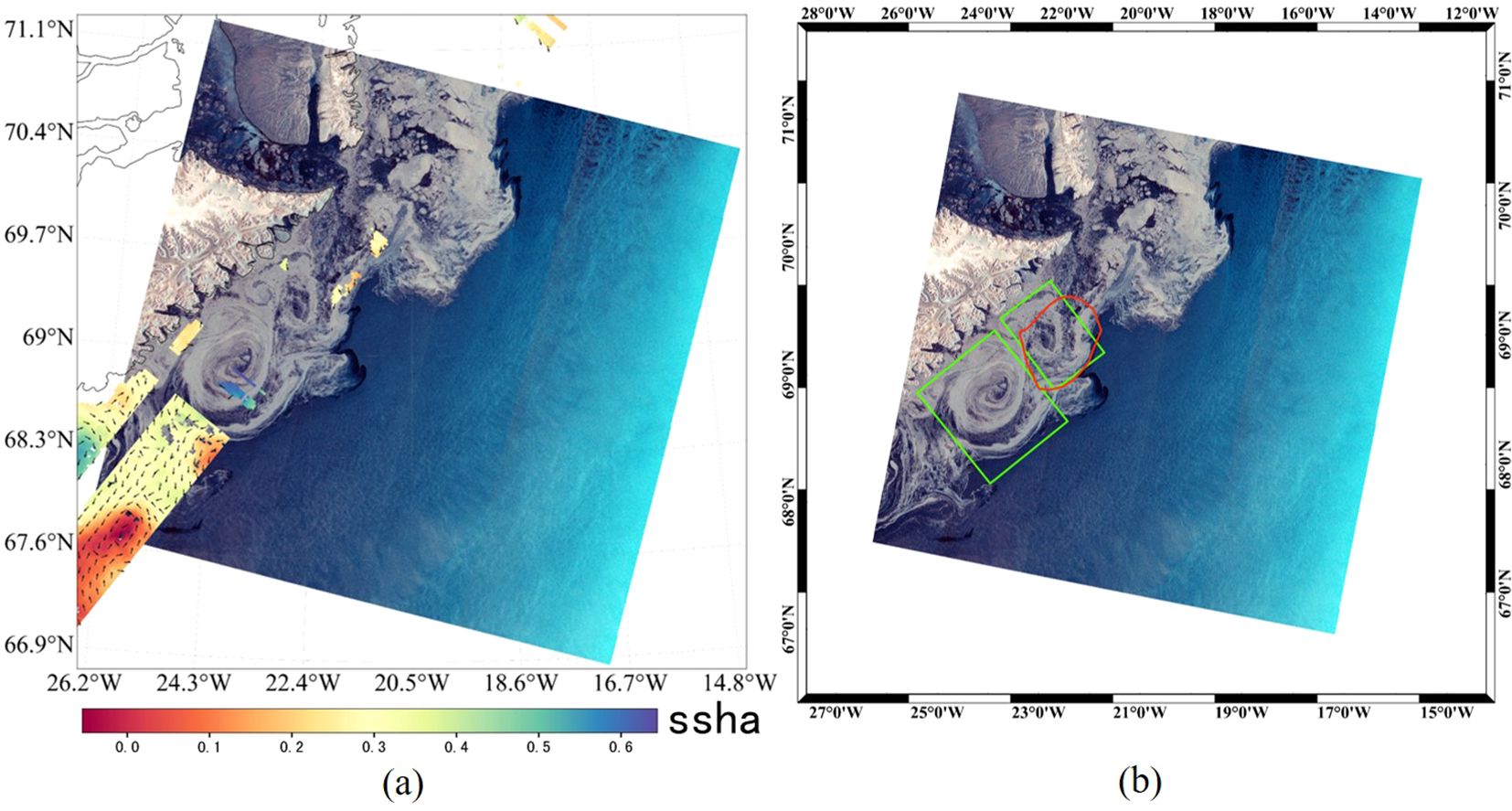
Figure 14. Comparison of the ice eddy identification results from OIEDNet (green) with those obtained from SWOT and the mesoscale eddy track atlas product META3.1exp DT (red). (A, B) data time are S1: 2023-11-03 08:05:21 UTC. SWOT: 2023-11-03 16:46:19 UTC, META3.1exp DT: 2023-11-03 UTC.

The ice eddies detected by OIEDNet were compared and validated against in situ data collected from OpenMetBuoys-v2021 (OMBs) deployed in the marginal ice zone. Figure 15 illustrates the movement trajectories of two ice buoys in the marginal ice zone around Svalbard from August 18, 2022, to August 26, 2022. Red triangles are used to denote the starting positions of the buoys, while pentagrams indicate the ending positions of their trajectories. The ice buoy trajectories exhibit a counterclockwise rotation consistent with the direction of the ice eddy, indicating a cyclonic ice eddy.

Figure 15

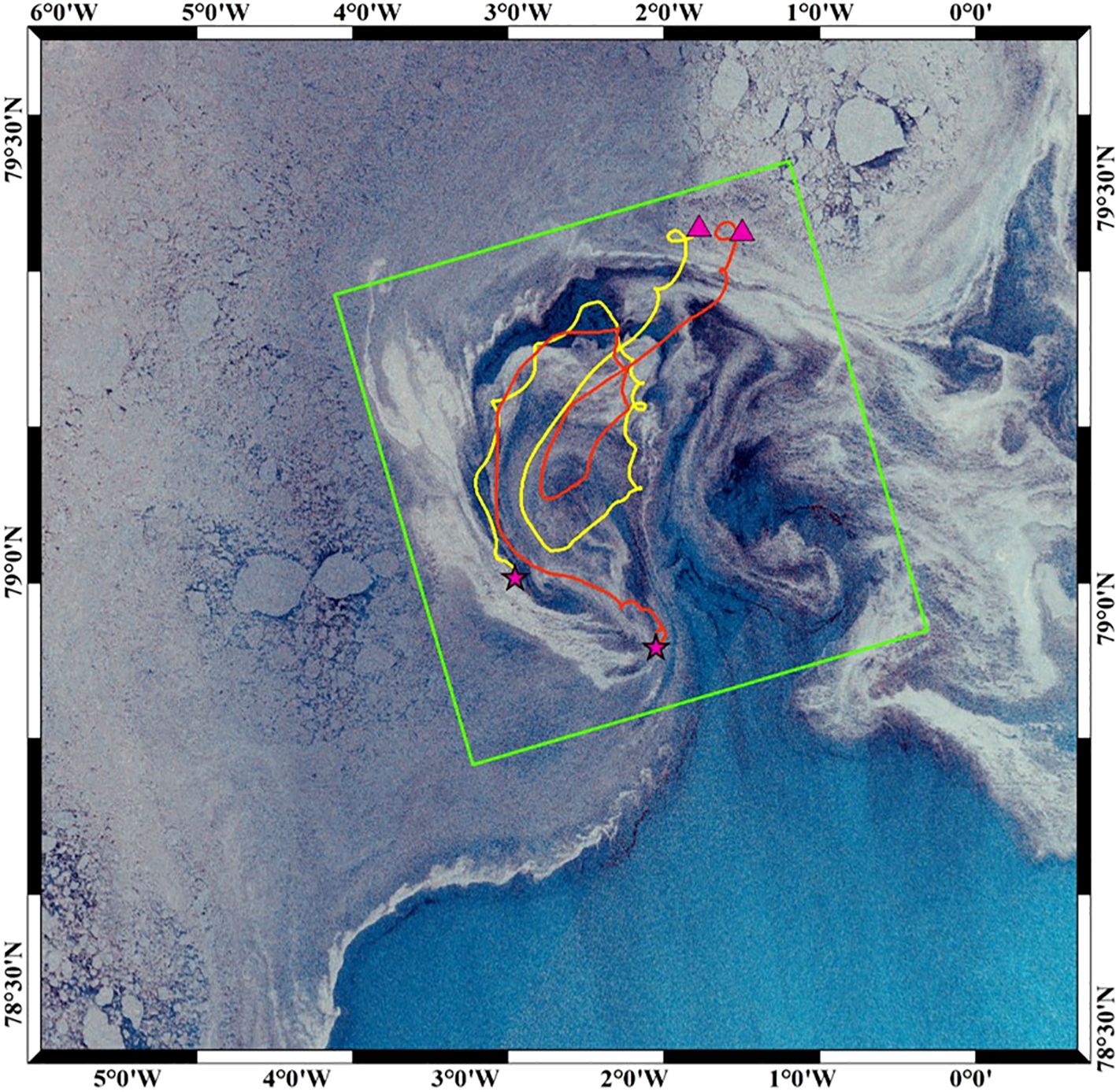
Figure 15. Comparison of the ice eddy identification results from OIEDNet (green) with those obtained from OMBs (red and yellow). The acquisition time for Sentinel-1 occurred on August 23, 2022, at 07:53:58 UTC. OMBs data collection spanned from August 18, 2022, to August 26, 2022, between 07:53:58 and 07:55:02 UTC. Red triangles are used to denote the starting positions of the buoys, while pentagrams indicate the ending positions of their trajectories.

4.4 Spatial and temporal distribution of ice eddies

Using the OIEDNet ice eddy detection framework, ice eddy identification and scale information extraction were performed on 702 SAR images containing ice eddies in the Nordic Seas from January 2022 to December 2023. To ensure the accuracy of the statistical feature information of the ice eddies, the detected ice eddy types were annotated using a manual visual inspection method. A total of 2283 ice eddies were identified, including 1724 cyclonic eddies (CEs) and 559 anticyclonic eddies (AEs). The number of cyclonic ice eddies is 3.08 times that of anticyclonic eddies, which may be related to the mechanism of anticyclonic eddy generation and the interaction between the two (McWilliams, 2016).

The spatial density distribution of ice eddies was calculated using a 0.1° × 0.1° grid, as shown in Figure 16A, revealing that the densest distribution of ice eddies is located in the north-central Greenland Sea, which exhibits a high number of both cyclonic and anticyclonic ice eddies. The monthly variation is shown in Figure 16B, indicating that Nordic Seas ice eddies are present throughout the year, with two peaks in the total number of ice eddies in May and October, and a low in March. Overall, May to November is the period when ice eddies are most frequent. The formation of ice eddies in the Nordic Seas results from a combination of dynamical and thermal forces (Perovich and Jones, 2014). Spatially, areas of high ice eddy occurrence are often closely linked to the Arctic Current, with the East Greenland Cold Current flowing along the east coast of Greenland. Temporally, with the onset of the Arctic summer polar day, sea surface temperatures (SSTs) rise, and glacier melting causes the expansion of marginal ice areas, leading to high ice eddy occurrence. In contrast, the Nordic Seas ice cover decreases rapidly to reach a minimum at the beginning of October, after which the ice area starts to expand rapidly. Thus, the thermodynamic factors in the Nordic Seas are more complex in October, which is conducive to the formation of ice eddies.

Figure 16

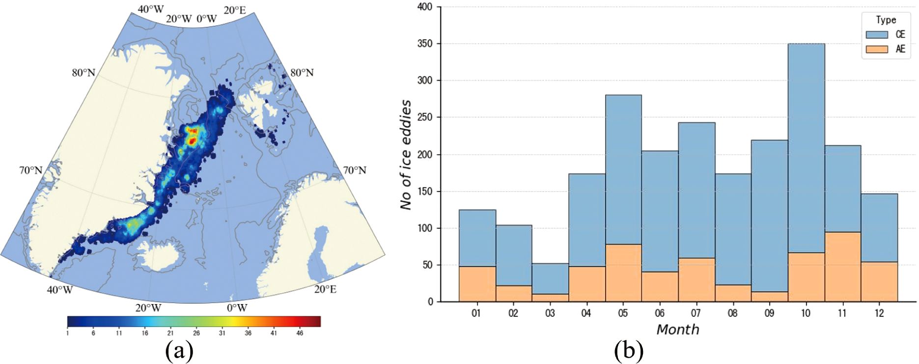
Figure 16. Spatial distribution of ice eddies with histograms of months. (A) The spatial distribution of ice eddy frequency (gray lines represent the 200 m and 2000 m bathymetry lines of IBCAOv4.0). (B) Monthly variation in the number of ice eddies detected during 2022-2023.

Figure 17A shows that the sizes of ice eddies in the Nordic Seas are primarily concentrated in the mesoscale and submesoscale intervals. The diameters of these eddies are mostly in the range of 10-100 km. The diameter of cyclonic ice eddies is mainly between 10-60 km, while the diameter of anticyclonic ice eddies is mostly between 30-70 km, indicating that anticyclonic ice eddies tend to be larger than cyclonic ice eddies. Large ice eddies are primarily located in the north-central Greenland Sea.

Figure 17

Figure 17. Histogram distributions of ice eddy number, ice eddy diameter, and wind velocity. (A) Distributions of the number and diameter of ice eddies, with cyclones shown in blue and anticyclones in orange. (B) Distributions of the number of ice eddies and wind velocity (m/s), based on data from the ERA5 Interim Reanalysis.

From Figure 17B, we observe that the proposed model maintains detection performance despite increasing wind velocity. Although the number of ice eddy detections decreases with higher wind speeds, this does not indicate a decline in model performance; instead, it reflects the inherent difficulty of eddy formation in areas with strong winds, resulting in a reduced number of eddies. The lack of a sharp downward trend in detections further illustrates the robustness of the proposed model across varying wind speeds. Regarding wind velocity, 79.7% of the detected ice eddies formed under low wind conditions of 1-4 m/s, while about 20.3% occurred under medium wind conditions. Similarly, from Figure 18, as ice concentration increases, the number of ice eddies decreases. The rate of detected ice eddies shows a gradual decline, which further demonstrates the robustness of the proposed model under varying ice concentrations.

Figure 18

Figure 18. Distribution of the number of ice eddies and their average diameter (km) across ice concentration (%) for cyclonic (blue) and anticyclonic (orange) ice eddies.

5 Conclusions

To accurately detect MIZs ice eddies, denoising algorithms and image processing techniques are combined to propose a high-quality RGB false-color image production method and to create a dual-polarization synthetic aperture radar false-color ice eddy dataset. Simultaneously, the OIEDNet ice eddy detection model was developed and trained, achieving a precision rate of 94.4% and a recall rate of 93.65%, highlighting significant advantages in ice eddy detection. The OIEDNet effectively detects dual-polarized SAR ice eddies with a small sample size, identifying Submesoscale and mesoscale ice eddies in SAR images quickly and accurately. The experimental results demonstrate that the ice eddies detected in SAR images are not as large as previously indicated. The experimental results show that the OIEDNet model excels at detecting dense eddy regions in ice eddy detection. The rotating detection frame of OIEDNet better fits the eddy, effectively avoiding overlap. The interaction between ocean circulation and currents involves the splitting and fusion of ocean eddies, leading to the multinuclear structure of ice eddies, which can be more accurately detected by the rotational detection method. The OIEDNet also significantly reduces the leakage of ice eddies and false detections, especially in dense eddy regions. The OIEDNet not only accurately detects ice eddies in the Arctic MIZs but also addresses the traditional HBB’s limitations in identifying ice eddies of different scales and forms. This work lays a solid foundation for future research on the automatic detection and quantification of ice eddies.

Despite the OIEDNet model’s high performance in ice eddy detection, certain limitations persist. For instance, minor changes in the rotation angle can lead to significant alterations in the detection frame, increasing instability and difficulty in the detection and regression process. Exploring new angle representations could reduce ambiguity. Furthermore, we will incorporate multi-polarization and multi-frequency SAR images for model training to enhance the accuracy of ice eddy detection. The identification of ice eddy drift using Synthetic Aperture Radar (SAR) images holds significant potential for enhancing the understanding of sea ice eddy dynamics.

Data availability statement

The datasets presented in this study can be found in online repositories. The names of the repository/repositories and accession number(s) can be found in the article/supplementary material.

Author contributions

JW: Data curation, Investigation, Methodology, Software, Validation, Writing – original draft, Conceptualization, Project administration, Visualization, Writing – review & editing. YZ: Software, Visualization, Writing – review & editing, Formal analysis. TW: Methodology, Writing – review & editing, Writing – original draft, Investigation. CM: Funding acquisition, Resources, Writing – review & editing, Investigation, Supervision, Project administration. GC: Funding acquisition, Methodology, Resources, Writing – review & editing, Conceptualization, Project administration, Supervision.

Funding

The author(s) declare financial support was received for the research, authorship, and/or publication of this article. This work was supported in part by Laoshan Laboratory Science and Technology Innovation Projects under Grant LSKJ202204301 and LSKJ202201302, the National Natural Science Foundation of China under Grant 42030406 and 42276179, and in part by the Taishan Scholars Program.

Conflict of interest

Authors JW and YZ were employed by Piesat Information Technology Co., Ltd.

The remaining authors declare that the research was conducted in the absence of any commercial or financial relationships that could be construed as a potential conflict of interest.

Publisher’s note

All claims expressed in this article are solely those of the authors and do not necessarily represent those of their affiliated organizations, or those of the publisher, the editors and the reviewers. Any product that may be evaluated in this article, or claim that may be made by its manufacturer, is not guaranteed or endorsed by the publisher.

References

Bashmachnikov I. L., Kozlov I. E., Petrenko L. A., Glok N. I., Wekerle C. (2020). Eddies in the north Greenland sea and fram strait from satellite altimetry, SAR and high-resolution model data. J. Geophysical Research: Oceans 125, e2019JC015832. doi: 10.1029/2019JC015832

Crossref Full Text | Google Scholar

Cassianides A., Lique C., Korosov A. (2021). Ocean eddy signature on sar-derived sea ice drift and vorticity. Geophysical Res. Lett. 48, e2020GL092066. doi: 10.1029/2020GL092066

Crossref Full Text | Google Scholar

Chelton D. B., Schlax M. G., Samelson R. M. (2011). Global observations of nonlinear mesoscale eddies. Prog. oceanography 91, 167–216. doi: 10.1016/j.pocean.2011.01.002

Crossref Full Text | Google Scholar

Ding J., Xue N., Long Y., Xia G.-S., Lu Q. (2019). “Learning RoI transformer for oriented object detection in aerial images,” in Proceedings of the IEEE/CVF conference on computer vision and pattern recognition. 2849–2858.

Google Scholar

Du Y., Liu J., Song W., He Q., Huang D. (2019a). Ocean eddy recognition in sar images with adaptive weighted feature fusion. IEEE Access 7, 152023–152033. doi: 10.1109/Access.6287639

Crossref Full Text | Google Scholar

Du Y., Song W., He Q., Huang D., Liotta A., Su C. (2019b). Deep learning with multi-scale feature fusion in remote sensing for automatic oceanic eddy detection. Inf. Fusion 49, 89–99. doi: 10.1016/j.inffus.2018.09.006

Crossref Full Text | Google Scholar

Dumont D., Kohout A., Bertino L. (2011). A wave-based model for the marginal ice zone including a floe breaking parameterization. J. Geophysical Research: Oceans 116. doi: 10.1029/2010JC006682

Crossref Full Text | Google Scholar

Fu L.-L., Holt B. (1983). Some examples of detection of oceanic mesoscale eddies by the SEASAT synthetic-aperture radar. J. Geophysical Research: Oceans 88, 1844–1852. doi: 10.1029/JC088iC03p01844

Crossref Full Text | Google Scholar

Gupta M., Thompson A. F. (2022). Regimes of sea-ice floe melt: Ice-ocean coupling at the submesoscales. J. Geophysical Research: Oceans 127, e2022JC018894. doi: 10.1029/2022jc018894

Crossref Full Text | Google Scholar

Han J., Ding J., Li J., Xia G.-S. (2021). Align deep features for oriented object detection. IEEE Trans. Geosci. Remote Sens. 60, 1–11. doi: 10.1109/TGRS.2021.3062048

Crossref Full Text | Google Scholar

Huang D., Du Y., He Q., Song W., Liotta A. (2017). “DeepEddy: A simple deep architecture for mesoscale oceanic eddy detection in SAR images,” in 2017 IEEE 14th International Conference on Networking, Sensing and Control (ICNSC). 673–678.

Google Scholar

Jakobsson M., Mayer L. A., Bringensparr C., Castro C. F., Mohammad R., Johnson P., et al. (2020). The international bathymetric chart of the arctic ocean version 4.0. Sci. Data 7, 176. doi: 10.1038/s41597-020-0520-9

PubMed Abstract | Crossref Full Text | Google Scholar

Johannessen J., Johannessen O., Svendsen E., Shuchman R., Manley T., Campbell W., et al. (1987). Mesoscale eddies in the fram strait marginal ice zone during the 1983 and 1984 marginal ice zone experiments. J. Geophysical Research: Oceans 92, 6754–6772. doi: 10.1029/JC092iC07p06754

Crossref Full Text | Google Scholar

Karimova S., Lavrova O. Y., Solov’Ev D. (2012). Observation of eddy structures in the baltic sea with the use of radiolocation and radiometric satellite data. Izvestiya Atmospheric oceanic Phys. 48, 1006–1013. doi: 10.1134/S0001433812090071

Crossref Full Text | Google Scholar

Khachatrian E., Sandalyuk N., Lozou P. (2023). Eddy detection in the marginal ice zone with sentinel-1 data using YOLOv5. Remote Sens. 15, 2244. doi: 10.3390/rs15092244

Crossref Full Text | Google Scholar

Korosov A. A., Rampal P. (2017). A combination of feature tracking and pattern matching with optimal parametrization for sea ice drift retrieval from SAR data. Remote Sens. 9, 258. doi: 10.3390/rs9030258

Crossref Full Text | Google Scholar

Kozlov I. E., Artamonova A. V., Manucharyan G. E., Kubryakov A. A. (2019). Eddies in the western arctic ocean from spaceborne SAR observations over open ocean and marginal ice zones. J. Geophysical Research: Oceans 124, 6601–6616. doi: 10.1029/2019JC015113

Crossref Full Text | Google Scholar

Kozlov I. E., Atadzhanova O. A. (2021). Eddies in the marginal ice zone of fram strait and svalbard from spaceborne SAR observations in winter. Remote Sens. 14, 134. doi: 10.3390/rs14010134

Crossref Full Text | Google Scholar

Li K., Wan G., Cheng G., Meng L., Han J. (2020). Object detection in optical remote sensing images: A survey and a new benchmark. ISPRS J. photogrammetry Remote Sens. 159, 296–307. doi: 10.1016/j.isprsjprs.2019.11.023

Crossref Full Text | Google Scholar

Lin T.-Y., Dollár P., Girshick R., He K., Hariharan B., Belongie S. (2017). “Feature pyramid networks for object detection,” in Proceedings of the IEEE conference on computer vision and pattern recognition. 2117–2125.

Google Scholar

Liu L., Ouyang W., Wang X., Fieguth P., Chen J., Liu X., et al. (2020). Deep learning for generic object detection: A survey. Int. J. Comput. Vision 128, 261–318. doi: 10.1007/s11263-019-01247-4

Crossref Full Text | Google Scholar

Liu S., Qi L., Qin H., Shi J., Jia J. (2018). “Path aggregation network for instance segmentation,” in Proceedings of the IEEE conference on computer vision and pattern recognition. 8759–8768.

Google Scholar

Ma J., Shao W., Ye H., Wang L., Wang H., Zheng Y., et al. (2018). Arbitrary-oriented scene text detection via rotation proposals. IEEE Trans. multimedia 20, 3111–3122. doi: 10.1109/TMM.2018.2818020

Crossref Full Text | Google Scholar

Manucharyan G. E., Thompson A. F. (2017). Submesoscale sea ice-ocean interactions in marginal ice zones. J. Geophysical Research: Oceans 122, 9455–9475. doi: 10.1002/2017JC012895

Crossref Full Text | Google Scholar

McWilliams J. C. (2016). Submesoscale currents in the ocean. Proc. R. Soc. A: Mathematical Phys. Eng. Sci. 472, 20160117. doi: 10.1098/rspa.2016.0117

PubMed Abstract | Crossref Full Text | Google Scholar

Nurser A., Bacon S. (2013). Eddy length scales and the rossby radius in the arctic ocean. Ocean Sci. Discussions 10.5, 1807–1831. doi: 10.5194/osd-10-1807-2013

Crossref Full Text | Google Scholar

Park J.-W., Korosov A. A., Babiker M., Sandven S., Won J.-S. (2017). Efficient thermal noise removal for sentinel-1 TOPSAR cross-polarization channel. IEEE Trans. Geosci. Remote Sens. 56, 1555–1565. doi: 10.1109/TGRS.2017.2765248

Crossref Full Text | Google Scholar

Perovich D. K., Jones K. F. (2014). The seasonal evolution of sea ice floe size distribution. J. Geophysical Research: Oceans 119, 8767–8777. doi: 10.1002/2014JC010136

Crossref Full Text | Google Scholar

Qiu Y., Li X. (2022). Retrieval of sea ice drift from the central arctic to the fram strait based on sequential sentinel-1 SAR data. IEEE Trans. Geosci. Remote Sens. 60, 1–14. doi: 10.1109/TGRS.2022.3226223

Crossref Full Text | Google Scholar

Rabault J., Taelman C., Idžanović M., Hope G., Nose T., Kristoffersen Y., et al. (2024). An openmetbuoy dataset of marginal ice zone dynamics collected around svalbard in 2022 and 2023. arXiv. doi: 10.48550/arXiv.2409.04151

Crossref Full Text | Google Scholar

Sun Y., Li X. (2020). Denoising sentinel-1 extra-wide mode cross-polarization images over sea ice. IEEE T. Geosci. Remote. 3, 2116–2131. doi: 10.20944/preprints202006.0092.v1

Crossref Full Text | Google Scholar

Toole J. M., Krishfield R. A., Timmermans M.-L., Proshutinsky A. (2011). The ice-tethered profiler: Argo of the arctic. Oceanography 24, 126–135. doi: 10.5670/oceanog.2011.64

Crossref Full Text | Google Scholar

Varghese R., Sambath M. (2024). “Yolov8: A novel object detection algorithm with enhanced performance and robustness,” in 2024 International Conference on Advances in Data Engineering and Intelligent Computing Systems (ADICS). 1–6.

Google Scholar

von Appen W.-J., Wekerle C., Hehemann L., Schourup-Kristensen V., Konrad C., Iversen M. H. (2018). Observations of a submesoscale cyclonic filament in the marginal ice zone. Geophysical Res. Lett. 45, 6141–6149. doi: 10.1029/2018GL077897

Crossref Full Text | Google Scholar

Xia G.-S., Bai X., Ding J., Zhu Z., Belongie S., Luo J., et al. (2018). “DOTA: A large-scale dataset for object detection in aerial images,” in Proceedings of the IEEE conference on computer vision and pattern recognition. 3974–3983.

Google Scholar

Xia L., Chen G., Chen X., Ge L., Huang B. (2022). Submesoscale oceanic eddy detection in SAR images using context and edge association network. Front. Mar. Sci. 9, 1023624. doi: 10.3389/fmars.2022.1023624

Crossref Full Text | Google Scholar

Yang X., Yang J., Yan J., Zhang Y., Zhang T., Guo Z., et al. (2019). “Scrdet: Towards more robust detection for small, cluttered and rotated objects,” in Proceedings of the IEEE/CVF international conference on computer vision. 8232–8241.

Google Scholar

Zhang D., Gade M., Wang W., Zhou H. (2023). EddyDet: A deep framework for oceanic eddy detection in synthetic aperture radar images. Remote Sens. 15, 4752. doi: 10.3390/rs15194752

Crossref Full Text | Google Scholar

Zhang D., Gade M., Zhang J. (2020). “Sar eddy detection using mask-rcnn and edge enhancement,” in IGARSS 2020-2020 IEEE international geoscience and remote sensing symposium. 1604–1607.

Google Scholar

Zheng P., Chong J., Wang Y. (2018). A method of automatic shape depiction and information extraction for oceanic eddies in sar images. J. Measurement Sci. Instrumentation 9, 241. doi: 10.3969/j.issn.1674-8042.2018.03.006

Crossref Full Text | Google Scholar

Zheng G., Songtao L., Feng W., Zeming L., Jian S. (2021). Yolox: Exceeding yolo series in 2021. arXiv. doi: 10.48550/arXiv.2107.08430

Crossref Full Text | Google Scholar

Zi N., Li X.-M., Gade M., Fu H., Min S. (2024). Ocean eddy detection based on yolo deep learning algorithm by synthetic aperture radar data. Remote Sens. Environ. 307, 114139. doi: 10.1016/j.rse.2024.114139

Crossref Full Text | Google Scholar