Full-grid bathymetry estimation in the numerical simulation of 8 tidal constituents using an ensemble adjustment Kalman filter-smoothing scheme

The spatially varying geographic-parameters introduce significant uncertainty into the ocean model. Due to the impracticality of manually tuning spatial varying parameters, data assimilation methods are widely used for geographic-parameter optimization (GPO). Practically, the limited observations do not contain enough information to perform GPO directly on the entire grid. Therefore, techniques are required to reduce the complexity of the parameters. A full-grid GPO scheme based on the ensemble adjustment Kalman filter (EAKF) is developed. Via smoothing the spatial distribution of posterior parameter members, the EAKF-smoothing (EAKF-S) introduces additional spatial correlations among parameters. Meanwhile, the small-scale correlation between the state and the parameters, which exhibit strong pseudo-correlations, is filtered out. A tide model of the Bohai Sea and Yellow Sea, considering 8 principal tidal constituents. is constructed using the Princeton Ocean Model with the generalized coordinate system (POMgcs). The EAKF-S is employed for optimizing the full-grid bathymetry. In twin experiment, based on idealized water level observations, EAKF-S effectively reduced model errors and approximately inverted the “true” bathymetry. After GPO, the lowest mean absolute error of the parameter ensemble is 0.83 m. A series of practical GPO experiments based on synthetic water level observations calculated from NAO.99Jb data are performed. First, the improvement of EAKF-S in accuracy and efficiency over standard EAKF is proven using an M₂ tide model. After that, a practical experiment on an 8 constituents tide model is performed. The results show that the forecasting performance of all 8 constituents is improved after GPO, indicating the efficacy of EAKF-S.

1 Introduction

Numerical models are the primary means for conducting ocean forecasting and reanalysis. Parameters, such as bathymetry, bottom friction, and open boundary conditions, have a significant impact on the accuracy of the model. By introducing observations into numerical models, data assimilation (DA) methods—including four-dimensional variational data assimilation (4D-Var; Courtier and Talagrand, 1987; Talagrand and Courtier, 1987; Rabier et al., 2000; Stammer et al., 2002), ensemble Kalman filter (EnKF; Evensen, 1994, Evensen, 2004) and their derivative methods—allow for the optimization of model parameters (Panchang and O’Brien, 1989; Smedstad and O’Brien, 1991; Anderson, 2001; Aksoy et al., 2006). Geographic-parameter optimization (GPO) is one of the concerns in parameter optimization. Currently, there have been many studies on GPO based on DA methods (Lardner et al., 1993; Zhang and Lu, 2008; Zhang et al., 2011; Wu et al., 2012; Guo et al., 2017; Liang et al., 2023).

Bathymetry is one of the fundamental geographic-dependent parameters in ocean models. Due to limitations in observational technology, environmental factors, and other aspects, current bathymetric datasets still contain certain errors (Li et al., 2023). In tide simulation, bathymetry significantly affects all state variables: water level, eastward and northward current velocities. This means that there is a strong correlation between bathymetry and both water levels and current. Based on observations of water levels or current velocities, the inversion of bathymetry can be achieved through the correlations between bathymetry and state variables revealed by the model. The key challenge of GPO for bathymetry lies in the vast number of parameters to be estimated. The ideal quantity of bathymetry parameters should match the number of 2-dimensional grid points. As the number of parameters increases, the uncertainty of the model will rapidly increase. Practically, the available observational information usually does not adequately match such finely tuned spatial parameter settings (Das and Lardner, 1991). This makes it difficult to achieve a deterministic solution to the optimization problem. To address the discrepancy between the large number of bathymetry parameters and the limited observations, researchers have employed various dimensionality reduction methods to meet practical requirements:

1. Partitioning the computational domain into blocks, where parameters within each block are considered constants (Das and Lardner, 1991; Lardner et al., 1993; Han et al., 2006).

2. Selecting independent parameter points within the computational domain for optimization. Parameter values at other grid points are determined by interpolation (Heemink et al., 2002).

3. Incorporating spatial correlation information of parameters into the background error covariance matrix. For instance, Wilson et al., 2010; Wilson and Özkan-Haller2012; Wilson et al, 2014 established a spatial correlation function based on horizontal length scales and vertical variance. By defining the expected shape and scale of bathymetric features, additional information is introduced into the background error covariance. The full-grid bathymetry estimation of the EnKF is then achieved.

It is noting that approaches (1), (2) mentioned above require tailored treatments for specific problems. Meanwhile, despite being proficient in achieving full-grid GPO, approach (3) is constrained by static spatial correlations among parameters. As a result, the specific spatial patterns are predetermined, imposing limitations on the optimization results.

Another challenge in bathymetry estimation for tide models arises from the long-time scale evolutionary processes of the tide. To obtain the globally optimized parameters, DA methods requires sufficient observations over a long duration to capture long-period features. 4D-Var establishes the correlation between state variables and parameters based on the adjoint model. Via the minimization time window aligned with the duration of oceanic processes, 4D-Var can fully capture the temporal features. However, 4D-Var requires numerous iterations of model integration. Moreover, the extensive amounts of both model and observational data pose challenges to computational memory. In contrast, the ensemble-based DA methods, such as EnKF, store the information of the model and observations within the ensemble distribution. As the model integrating, the ensemble dynamically determines the correlations between state variables and parameters. Although ensemble-based DA methods don’t retain all temporal information as 4D-Var does, they avoid the issue of memory limitations. Through parallelization, the computation time of ensemble-based DA methods can also be greatly reduced as well. Hence, ensemble-based DA methods are suitable for optimizing parameters over long periods. However, employing ensemble-based DA for parameter optimization requires setting an ensemble size at least equal to the number of parameters. Conducting parameter optimization on the entire grid directly is impractical. Therefore, it remains necessary to employ appropriate techniques to reduce the required ensemble size.

In this paper, an GPO scheme based on ensemble adjustment Kalman filter (EAKF; Anderson, 2001, Anderson, 2003) is developed. By incorporating a spatial smoothing term after the standard EAKF procedure, this EAKF-smoothing (EAKF-S) scheme enables full-grid GPO with a limited number of ensemble members. This enhancement not only improves the robustness of the EAKF, but also broadens its applicability to scenarios with limited observations. Additionally, the smoothing term effectively filters out small-scale correlations between observations and the background. Then, the EAKF can focus solely on the large and medium-scale patterns of observations. As a result, the complexity of GPO is reduced. The Princeton Ocean Model with a generalized coordinate system (POMgcs; Blumberg and Mellor, 1987; Ezer and Mellor, 2004) was used to conduct GPO experiments for bathymetry. A tide model for the Bohai Sea and Yellow Sea, including 4 semi-diurnal tidal constituents (M₂, S₂, N₂ and K₂), and 4 diurnal tidal constituents (K₁, O₁, P₁ and Q₁), was developed. The effectiveness and performance of EAKF-S were validated through both idealized twin experiment and a series of practical experiments. Water levels from POMgcs and those generated from the 1/12° tidal harmonic constants dataset NAO.99Jb (Matsumoto et al., 2000; https://www.miz.nao.ac.jp/staffs/nao99/index_En.html) were used as observations in twin and practical experiments, respectively.

The remainder of this paper is organized as follows: Section 2 introduces the POMgcs model and configurations. In Section 3, the formulations of the EAKF-S and the procedure of GPO experiments are described in detail. The twin experiment setups and the results are introduced in Section 4. The practical experiments based on NAO.99Jb observations are performed in Section 5. The last section gives a summary and discussion of GPO experiments.

2 The numerical model

2.1 Governing equations of POMgcs

Here, the external mode of the POMgcs is used to build the Bohai Sea and Yellow Sea tide model (referred to as “BYM”). The attributes of POMgcs model include a mixed coordinate system that makes the z-coordinate and sigma-coordinate compatible. The Arakawa C scheme is implemented for the horizontal grid, while the leap-frog scheme is used for time differencing. The free surface and split time step method is adopted. The two-dimensional external mode uses a short time step for a high-accuracy surface simulation. Meanwhile, the three-dimensional internal mode uses a longer time step to reduce the computational cost. In this paper, the vertical procedure is not considered. The governing equations are as follows:

$\begin{array}{ll}\frac{\partial \zeta }{\partial t}+\frac{\partial UD}{\partial x}+\frac{\partial VD}{\partial y}=0& (1)\end{array}$

$\begin{array}{ll}\begin{array}{l}\frac{\partial UD}{\partial t}+\frac{\partial U^{2}D}{\partial x}+\frac{\partial UVD}{\partial y}-fVD=-ɡD\frac{\partial \zeta }{\partial x}+\frac{{\rho }_a{C}_d{W}_x\sqrt{W_x^2+W_y^2}}{{\rho }_w}\\ -C_{b}U\sqrt{U^2+V^2}+\frac{\partial }{\partial x}\left(H^2{A}_M\frac{\partial U}{\partial x}\right)+\frac{\partial }{\partial y}\left[H{A}_M\left(\frac{\partial U}{\partial y}+\frac{\partial V}{\partial x}\right)\right]\end{array}& (2)\end{array}$

$\begin{array}{ll}\begin{array}{l}\frac{\partial VD}{\partial t}+\frac{\partial UVD}{\partial x}+\frac{\partial V^{2}D}{\partial y}+fUD=-ɡD\frac{\partial \zeta }{\partial y}+\frac{{\rho }_a{C}_d{W}_y\sqrt{W_x^2+W_y^2}}{{\rho }_w}\\ -C_{b}V\sqrt{U^2+V^2}+\frac{\partial }{\partial y}\left(H^2{A}_M\frac{\partial V}{\partial y}\right)+\frac{\partial }{\partial x}\left[H{A}_M\left(\frac{\partial U}{\partial y}+\frac{\partial V}{\partial x}\right)\right],\end{array}& (3)\end{array}$

where $t$ is the model time step; $x$ and $y$ are the conventional cartesian coordinates; $U$ and $V$ are the vertically averaged velocity components; $D=H+\text{ζ}$, where the $\text{ζ}$ is the water level, $H$ is the bathymetry; $f$ is the Coriolis frequency, which takes the local value; $ɡ$ is the gravitational acceleration; ${\rho }_a$ and ${\rho }_w$ are the densities of the air and water, respectively; $C_d$ is the wind drag coefficient; $W_x$ and $W_y$ are the horizonal wind velocity components; $C_b$ is the coefficient of bottom friction; $A_M$ is the horizontal eddy viscosity.

2.2 Model settings

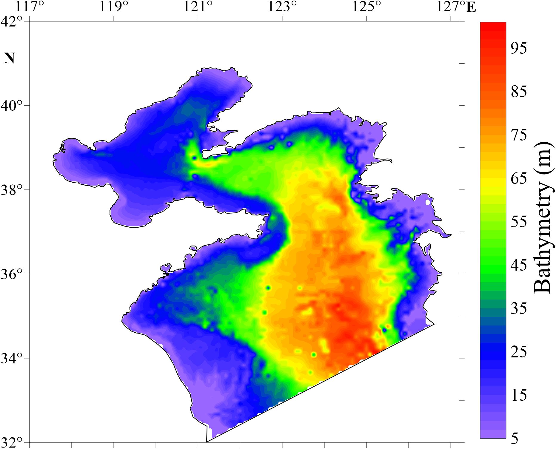
As shown in Figure 1, the model area extends from 32°N to 42°N in latitude and from 117°E to 127.2°E in longitude. In this continental shelf sea, tides are the predominant hydrodynamic influence in the model area. The gridded bathymetry is derived through interpolation of ETOPO5 bathymetry datasets (https://www.ncei.noaa.gov/products/etopo-global-relief-model). To prevent the occurrence of dry cells ($D<0$), the model enforces a minimum bathymetry of 5 m. The spatial resolution is 1/30° in both the east and north directions, and the integration time step is 12 s, which satisfies the Courant-Friedrichs-Lewy (CFL) condition (Courant et al., 1967) and is sufficient to simulate all 8 tidal constituents. A static initial condition with zero sea surface height and current velocity is used to spin up the model. The southern open boundary condition is the tide height, which is specified by:

Figure 1

Figure 1. Bathymetry (m) of BYM based on ETOPO5 data.

$\begin{array}{ll}\zeta ={\displaystyle {\sum }_{ntides}^{n=1}{f}_n{A}_n\cos ({\omega }_{n}t+V_0{}_n+u_n-{ɡ}_n),}& (4)\end{array}$

where $ntides$ is the number of tidal constituents; $A_n$ and ${ɡ}_n$ are the amplitude and phase lag of the $n$th tidal constituent, respectively, which derived from NAO.99Jb datasets; ${\text{ω}}_n$ is the frequency of the $n$th tidal constituent; $V_0{}_n$ is astronomical phase originating from the tide-generating potential of the $n$th tidal constituent; $f_n$ and $u_n$ are the nodal factor and correction angle of the $n$th tidal constituent, respectively.

Fan et al. (2019) demonstrated that the value of bottom friction coefficient in the east China shelf seas varies from 0.001 to 0.003. Therefore, the bottom friction coefficient of BYM is set to a constant value of 0.001. Additionally, forcing terms from the sea surface, such as wind stress, heat flux, and precipitation, are not considered in the BYM.

3 Methodology

3.1 Standard ensemble adjustment Kalman filter

In this paper, a deterministic EAKF based on the least squares approach is employed (Anderson and Anderson, 2001; Tippett et al., 2003). The implementation consists of 2 steps:

For a single observation $y^o$, the adjustments of the $k$th ensemble member of $y^o$ is first computed by:

$\begin{array}{ll}\text{Δ}{y}_k^o=\left(\sqrt{\frac{{({\text{σ}}^o)}^2}{{({\text{σ}}^o)}^2+{({\text{σ}}_y^p)}^2}}-1\right)\left(y_k^p-{\overline{y}}^p\right)+\frac{{({\text{σ}}_y^p)}^2}{{({\text{σ}}^o)}^2+{({\text{σ}}_y^p)}^2}\left(y^o-{\overline{y}}^p\right),& (5)\end{array}$

where ${\text{σ}}^o$ and ${\text{σ}}_y^p$ denote the standard deviation of observational error and prior standard deviation of $y^o$, respectively; $y_k^p$ is the $k$th prior ensemble member of $y^o$, which is obtained by spatial interpolation of the prior state variable; ${\overline{y}}^p$ denotes the ensemble mean of $y_k^p$.

Next, based on the correlations between $y_k$ and relevant state variables or parameters, the observational increment is projected as follows:

$\begin{array}{ll}{x}_k^a=x_k^p+r_{x,y}\frac{{\text{cov}}_{x,y}^p}{{({\text{σ}}_y^p)}^2}\text{Δ}{y}_k^o,& (6)\end{array}$

where $x_k^a$ and $x_k^p$ denote the $k$th posterior and prior ensemble member of state variable or parameter, respectively; ${\text{cov}}_{x,y}^p$ is the covariance between the state variable or parameter and the observation; $r_{x,y}$ is the localization factor, which is determined by the Gaspari-Cohn function (Gaspari and Cohn, 1999):

$\begin{array}{ll}{r}_{x,y}=\{\begin{array}{ll}-\frac{1}{4}{(\frac{b}{a})}^5+\frac{1}{2}{(\frac{b}{a})}^4+\frac{5}{8}{(\frac{b}{a})}^3-\frac{5}{3}{(\frac{b}{a})}^2+1,& \hfill 0\le b\le a\hfill \\ \frac{1}{12}{(\frac{b}{a})}^5-\frac{1}{2}{(\frac{b}{a})}^4+\frac{5}{8}{(\frac{b}{a})}^3+\frac{5}{3}{(\frac{b}{a})}^2-5(\frac{b}{a})+4-\frac{2}{3}{(\frac{b}{a})}^{-1},& \hfill a<b\le 2a\hfill \\ 0,& \hfill b>2a\hfill \end{array}& (7)\end{array}$

where $a$ represents the empirically specified impact radius; $b$ denotes the spatial distance between $y^o$ and $x_k$.

EAKF measures the posterior uncertainty by standard deviation or ensemble spread. As EAKF progresses, the posterior uncertainty consistently becomes smaller than the prior uncertainty. In other words, the ensemble spread gradually decreases. The model biases introduce an underestimation of the prior state uncertainty, leading to an overestimation of model accuracy. Consequently, the effect of the assimilation will progressively weaken and may even lead to filter divergence. Therefore, state and parameter inflation need to be introduced before the EAKF. For state variables, a static multiplicative inflation scheme is applied. A constant inflation factor is determined to inflate perturbations of each ensemble member relative to the ensemble mean. As for parameters, a conditional static inflation scheme is introduced (Aksoy et al., 2006; Tong and Xue, 2008). For the ensemble of a single parameter, the inflation is calculated as follows:

$\begin{array}{ll}\widetilde{P_m}=\overline{P}+\max (1,\frac{{\text{α}}_0{\text{σ}}_0}{{\text{σ}}_t})(P_m-\overline{P}),& (8)\end{array}$

where $P_m$ and $\widetilde{P_m}$ denote the parameter ensemble before and after inflation, respectively; $\overline{P}$ is the mean of $P_m$; ${\text{α}}_0$ is the empirically set inflation factor; ${\text{σ}}_0$ and ${\text{σ}}_t$ are the standard deviation of P_m at the initial time step and the $t$th time step.

3.2 Framework of EAKF-smoothing

As illustrated by Equation 5, the EAKF linearly adjusts $y^p$ based on the mean and variance of prior ensemble. Subsequently, via the local least squares fitting outlined in Equation 6, the adjustment is projected onto the gridded state variables and parameters (Zhang and Lu, 2008). Both steps ignore the higher-order nonlinear correlations of the ensemble. Hence, due to the strong nonlinearity correlation between parameters and state variables, certain errors arise in the adjustment by EAKF. Moreover, constrained by the ensemble size and the spatial scale of observations, pseudo-correlations unavoidably arise in the covariance between the background and observations. Under the conditions of full-grid parameter optimization, the projection of the observational increments affects all grid points. Therefore, the scale of forementioned error signals can reach the level of model resolution. Consequently, although observations may indeed contain small spatial scale information, it is hard for EAKF to accurately identify them. Therefore, filtering out small-scale information, relying solely on EAKF adjustments at relatively large scales should yield better effects.

After conducting parameter optimization with the standard EAKF, both large and small spatial scale information are projected onto the posterior parameter. Applying the smoothing term individually to each parameter member can effectively remove small scale information. To control the smoothing scale, we adopt the cost function proposed by Li et al, 2008; Li et al, 2013 for the multigrid analysis (MGA) method as the smoothing term. For a one-dimensional with $M$ homogeneous distributed grid points, the smoothing term can be described as:

$\begin{array}{ll}{P}^{T}SP={\displaystyle {\sum }_{M-1}^{i=2}{(P_{i-1}-2·P_i+P_{i+1})}^2},& (9)\end{array}$

Where P is the parameter with dimension $M\times 1$; S is the smoothing matrix with dimension $M\times M$.

Equation 9 represents the square of the numerator of the second derivative at the $i$th point, which characterizes the smoothness of the grid point. However, if Equation 9 is used directly as the cost function for P, the optimal solution for the smoothing term would inevitably be a straight line. To constrain the smoothing scale, we draw on the form of the MGA observation term and incorporate the parameters before smoothing (P^b) into the cost function:

$\begin{array}{ll}J=\frac{1}{2}{P}^{T}SP+\frac{1}{2}{(P-P^b)}^T{O}^{-1}(P-P^b)& (10)\end{array}$

$\begin{array}{ll}O={\text{λ}}^2·(R\circ R),& (11)\end{array}$

Where $O$ represents the background weight matrix, which is determined by a smoothing coefficient $\text{λ}$ and the confidence matrix R of the parameters. Where $\text{λ}$ is empirically specified to prevent over-smoothing or under-smoothing, as $\text{λ}$ approaches 0, the smoothing term will have no effect, while as $\text{λ}$ approaches infinity, the smoothing term will cause the P to converge to a uniform vector (Supplementary Figure S4). Meanwhile, R is defined based on the sensitivity of the parameters.

Under the same observational increment, the EAKF adjusts parameters differently due to their sensitivities to the observational state variable. After scaling the observational increment based on sensitivity information, parameters with lower sensitivity will have larger adjustments. If parameters of all grids are smoothed with equal weights, the sensitivity information will also be penalized by the smoothing term. By introducing sensitivity information into the $O$ matrix, the smoothing term can account for the scaling adjustments. Given the infeasibility of accurately estimating the sensitivity of geographic-dependent parameters, we assume that these parameters are independent to each other. Meanwhile, the time-varying characteristics of parameter sensitivity are ignored. As a result, $\text{R}$ is represented as a static and diagonal matrix. For the full-grid bathymetry estimation of BYM, we assume that the BYM using the ETOPO5 data, without perturbation, is the unbiased model. The parameter sensitivity is approximately determined by the following scheme.

First, generate the perturbated bathymetry ensemble member:

1. Independent points are selected every 10 grid points in the east and north directions. Each selected point is assigned a Gaussian random number with a mean of 0 and a standard deviation of 10% of the local bathymetry to generate a spatially coarsened perturbation.

2. Using the coarsened perturbation, the full-grid bathymetry perturbation distribution is obtained through bilinear interpolation.

3. Combine the perturbation distribution with the ETOPO5 bathymetry data to generate the perturbated bathymetry member.

The approach above guarantees significant state differences while preventing the occurrence of dry cells. 50 bathymetry members are generated, each forecasting for 35 days. The first 5 days are for spin-up, the subsequent 30 days of the forecast water level are saved to estimate the sensitivity. The root mean square error (RMSE) of the water level between the ensemble members and the unbiased model is calculated to quantify parameter sensitivity, for the $t$th hour, the RMSE of the grid point $(i,j)$ is:

$\begin{array}{ll}RMSE(i,j,t)=\sqrt{\frac{{\sum }_{k=1}^M{({\text{ζ}}_k(i,j)-{\text{ζ}}_{unbiased}(i,j))}^2}{M}},& (12)\end{array}$

where $M$ is the number of the ensemble members; ${\text{ζ}}_k$ and ${\text{ζ}}_{unbiased}$ are the water level of the $k$th ensemble member and the unbiased model, respectively.

Then, to filter out the temporal variation in parameter sensitivity and for better quantification of parameter sensitivity in the cost function, the RMSE is time-averaged and normalized:

$\begin{array}{ll}TRMSE(i,j)=\frac{{\sum }_{t=1}^{N}RMSE(i,j,t)}{N}& (13)\end{array}$

$\begin{array}{ll}NRMSE(i,j)=\frac{TRMSE(i,j)-TRMS{E}_{\text{min}}}{TRMS{E}_{\text{max}}-TRMS{E}_{\text{min}}},& (14)\end{array}$

where $TRMSE$ and $NRMSE$ are the time-averaged RMSE and normalized $TRMSE$, respectively; $N$ is the total number of integrated hours; $TRMS{E}_{\text{max}}$ and $TRMS{E}_{\text{min}}$ represent the maximum and minimum of $TRMSE$ values among all grid points, respectively.

Here, the static confidence matrix $\text{R}$ can be generated with the $NRMSE$, for the bathymetry estimation of BYM, the confidence of single parameter on the grid point $(i,j)$ can be calculated as follows:

$\begin{array}{ll}R(i,j)=0.05\times (H(i,j)-5)\times (1-NRMSE(i,j))+0.5,& (15)\end{array}$

where the coefficient 5 is the minimum bathymetry; the coefficient 0.5 guarantees that $R(i,j)$ is greater than 0.5 and does not reach 0; the coefficient 0.05 is a manually defined factor to adjust the magnitudes of ${(P-P^b)}^T{O}^{-1}(P-P^b)$ and $P^{T}S\text{P}$, aiming to make them comparable in scale.

The spatial distribution of $R$ displays in Supplementary Figure S2. For a parameter with low sensitivity, the $NRMSE$ is smaller. The observational increment is relatively amplified by the sensitivity information. Hence, a larger uncertainty should be assigned to the smoothing term. Additionally, the value of the RMSE is proportional to the given parameter error. Therefore, in areas with greater bathymetry, the value of $NRMSE$ is also larger. To remove the impact of bathymetry, the $H(i,j)$ is considered in the Equation 14.

As can be seen from Equations 12–15, the $\text{R}$ matrix proposed in this paper is only a very rough estimate. Yet, there are still significant improvements in the experiments described in Section 5.1.

The limited-memory quasi-Newton method (L-BFGS) is employed to calculate the minimization of Equation 10, the gradient with respect to $\text{P}$ is expressed as:

$\begin{array}{ll}\nabla J=(S+O^{-1})P-O^{-1}{P}^b,& (16)\end{array}$

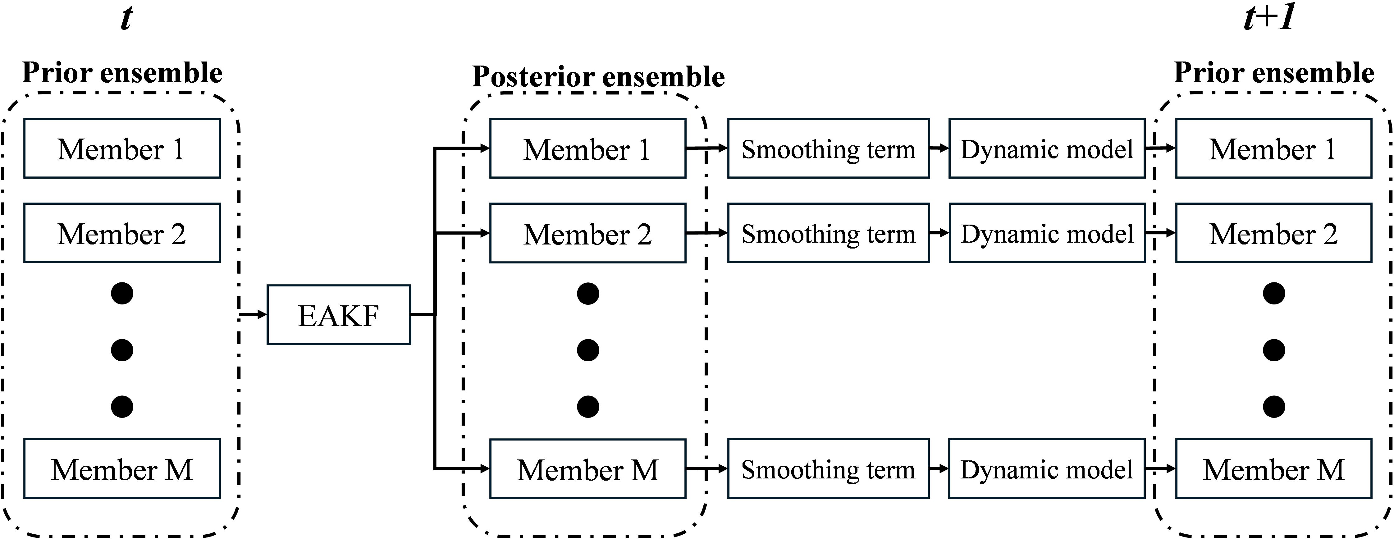
Figure 2 shows the brief procedure of the EAKF-S scheme from time $t$ of observation to the next time step $t+1$. During the linear projection of the observational increments, the EAKF adjusts both state variables and parameters based on their correlation with the observed state variables. As shown in Figure 2, after applying the smoothing term, the model forecasting restarts based on the smoothed parameters. The correlation between parameters and state variables can still be accurately estimated by the ensemble distribution. Therefore, the smoothing term can be well embedded into the EAKF algorithm.

Figure 2

Figure 2. The flowchart of EAKF-S from time $t$ of observation to the next forecast time step.

3.3 Settings of bathymetry estimation experiments

Following the scheme in Han et al. (2006), we perform the GPO experiments on the bathymetry increment parameters (BIP). For the $n$th ensemble member, the total bathymetry on the grid point $(i,j)$ is calculated as follows:

$\begin{array}{ll}{H}_n(i,j)=H_{ETOPO5}(i,j)+\text{Δ}{H}_n(i,j),& (17)\end{array}$

where the $\text{Δ}{H}_n$ denotes the BIP; $H_{ETOPO5}$ is the bathymetry obtained from the ETOPO5 dataset.

By introducing the BIP, the details of the ETOPO5 dataset can be well preserved during the smoothing of parameters. The BIPs that are on the grid points where the bathymetry of ETOPO5 greater than 5m were chosen. In the following GPO experiments, a total of 38440 BIPs, representing the number of parameters at the chosen grid points, were adjusted. We set 50 ensemble members for the BIPs. The perturbation of the bathymetry ensemble is generated using Gaussian random numbers, following the scheme of generating the perturbated bathymetry in Section 3.2. Furthermore, after generating the BIP ensemble, the smoothing term was applied to the ensemble members before forecasting. As demonstrated in the experiments detailed in Section 5.1, smoothing the initial BIP ensemble significantly accelerates the convergence of GPO and improves the stability of the EAKF-S. Based on a series of tests with impact radius ranging from 5 to 20 grids, state and BIP inflation factors from 1.0 to 1.1, by comparing the state RMSE, we set the impact radius $a$ (Equation 7) to Equation 15 grids, and both the state and BIP inflation factors were chosen as 1.05 in all experiments.

As an unconstrained method, EAKF can’t handle cases where parameters must stay within a reasonable range. For example, the BIP in this study must satisfy the condition $D>0$. Such problem can be resolved by manually adjust ensemble mean, when $D(i,j)<0$, the BIP ensemble will be adjusted according to:

$\begin{array}{ll}\text{Δ}H(i,j)=\text{Δ}{H}^a(i,j)-\min (\text{Δ}{H}^a(i,j))-1.5,& (18)\end{array}$

where $\text{Δ}{H}^a(i,j)$ represents the BIP ensemble on grid point $(i,j)$ after EAKF-S. Here, the members of $\text{Δ}H(i,j)$ are greater or equal to -1.5 m. Because of $H_{ETOPO5}(i,j)>5m$, the minimum bathymetry among ensemble members was constrained to be greater than 3.5 m, while the original distribution features of the ensemble are well preserved.

Due to the smoothing term, grid points are more likely to dry out within certain small areas. The overall tide pattern was not significantly impacted. Moreover, the parameter ensemble at the adjusted grid points still conforms to the characteristics of the original BIP distribution. The spin-up process of assimilation remains steady. After the spin-up phase, the EAKF forms a more accurate parameter-state correlation. Hence, the parameters deviating from the reasonable range should have disappeared or become very few. Using Equation 18 to adjust the remaining few parameters won’t significantly affect the accuracy of the GPO.

Note that the data assimilation scheme for enhancive parameter correction (DAEPC) has been applied to facilitate the performance of EAKF on GPO (Zhang et al., 2012). DAEPC starts parameter optimization after adjusting the state variables only (called state estimation only, SEO) until the data assimilation reaches a “quasi-equilibrium” stage. As the state error is relatively small, the parameter error, or the covariance between parameter and observation becomes the dominant signal. The effect of parameter optimization will be enhanced compared to performing state estimation and parameter optimization simultaneously.

In addition, the leap-frog time-stepping schemes in the POMgcs model generate the state of next time step by both current and the last time step. It will introduce significant inconsistency between the two steps if only the state of current time step is adjusted by the EAKF. Via project the observational increment on both time steps of the state variables, EAKF naturally allows for the matching between the 2 time steps (Zhang et al., 2004). This adjustment scheme was used for both water level and current during the experiments.

The steps for GPO experiments of EAKF-S are described below in Figure 3, followed by detailed explanations:

Figure 3

Figure 3. Flow chart of GPO experiments based on EAKF-S.

Step 1: Generate the coarsened BIP ensemble by the Gaussian random numbers.

Step 2: Interpolate the coarsened BIPs to obtain the full-grid BIP ensemble.

Step 3: Smooth the BIP members to get the initial BIP ensemble for the GPO experiments.

Step 4: Spin-up the BYM for 5 days to stabilize the model integration.

Step 5: When reached an observation time, the EAKF-S is applied to adjust the prior state variables and parameters based on DAEPC.

Step 6: After the EAKF-S, continue the model integration with the posterior state and BIPs.

Step 7: Repeat the Step 5 and Step 6 until the last time step.

4 The twin experiment

4.1 Experiment settings

In this section, the twin experiment of bathymetry estimation is conducted to evaluate the performance of EAKF-S. The 8 main tidal constituents of Bohai Sea and Yellow Sea are included in the BYM. The simulated water level, based on the ETOPO5 dataset as bathymetry, is considered as the “true” water level. The hourly, 1/10° observations are directly sampled from the “true” water level data. According to the accuracy of bathymetry datasets, we assume an error of approximately 10% of the local bathymetry. 0.1 times the model bathymetry was smoothed using Equation 10, with a $\text{λ}$ of 1 and the elements of $\text{R}$ setting to 0.01 times the model bathymetry. Then, add the smoothed 0.1 times bathymetry to the ETOPO5 bathymetry ($H_{ETOPO5}$) to create the biased BYM.

As the “true” water level is assimilated in the twin experiment, the standard deviation of observational error was set to a small constant of 0.05 m. Notably, the $\text{R}$ is set differently in Section 3.2 compared to when generating the biased BYM. As shown in Supplementary Figure S2, the range of elements in $\text{R}$ is approximately 0 to 4.5, while the range of 0.01 times model bathymetry is about 0 to 1. Since the $\text{S}$ in Equation 10 is static, in order to ensure that the smoothing term during assimilation and when generating the prior error are roughly consistent, λ is set to 0.2 when generating the biased model and performing EAKF-S. Based on the period of BYM and the computation time, the twin experiment was set to last 15.6 days. During the first 14 hours, only state estimation is performed, followed by jointly state and BIP estimation for the next 15 days.

4.2 Results

The time series of spatially averaged water level RMSE of the prior ensemble is displayed in Figure 4. The blue line represents the SEO while the red line is the GPO. According to the RMSE time series of SEO, we consider that the water level has reached the “quasi-equilibrium” state after the 14th hour. Therefore, in subsequent experiments, we set the duration of state estimation to 14 h. As shown in the figure, when state estimation was performed, the RMSE decreased from 0.1 m to 0.04 m. After the 14th hour, when the GPO started, the RMSE of water level rapidly decreased to 0.01 m within 12 h. The time series of RMSE then stabilized in the next 14.5 days, demonstrating the significant effectiveness of EAKF-S on the improvement of state error.

Figure 4

Figure 4. Time series of spatially averaged RMSE of prior water level, the red line is the GPO, the blue line is SEO, and the red dashed line represents the start time of GPO.

To evaluate the feasibility of EAKF-S in bathymetry inversion, the spatial distribution of Mean Absolute Error (MAE) of BIP members is calculated. Figure 5 shows the prior, “true”, and the posterior bathymetry, respectively. As shown in the figure, Figure 5C, which shows the ensemble mean of the posterior bathymetry, is significantly closer to the “true” bathymetry compared to the prior (Figure 5A). Figure 6 displays the spatial distribution of the prior BIP error (the smoothed 0.1-times-model bathymetry), and the $-\text{Δ}{H}_n$ of the posterior ensemble. The ensemble mean, The best member (with the minimum MAE) and the worst member (with the maximum MAE) are shown in Figures 6B–D, respectively. When $-\text{Δ}{H}_n$ and the prior error are consistent, it indicates that the posterior bathymetry is exactly the “true” bathymetry. We can see Figure 6B closely resembles Figure 6A. The spatial and time averaged RMSE of the forecast water level based on Figure 6B is 1.28 cm. An ensemble size of 50 suffices to capture the uncertainty of the prior bathymetry error. This can also be attributed to the well-chosen λ, which approximately aligns the smoothness of the prior error with the posterior BIPs. The initial knowledge of the parameter enables a better representation of the finer spatial features of the prior error. Conversely, even if the smoothing term is not set very precisely, EAKF-S can still achieve good results, demonstrating the robustness of the method. Figuress 6C, D illustrate the maximum differences among the BIP members. The MAE between Figure 6C and the prior error is 0.83 m, which is slightly larger than Figure 6A. Meanwhile, although Figure 6D has a relatively higher MAE of 2.03 m, its spatial and time-averaged RMSE remains a small value of 3.50 cm. On one hand, it indicates that diverse shapes of BIPs may all generate results close to the “true” water level. On the other hand, it also implies that the correlation between bathymetry and water level operates on a relatively large spatial scale.

Figure 5

Figure 5. The bathymetry of (A) the biased BYM, (B) the ETOPO5 bathymetry and (C) the ensemble mean of BIPs after GPO.

Figure 6

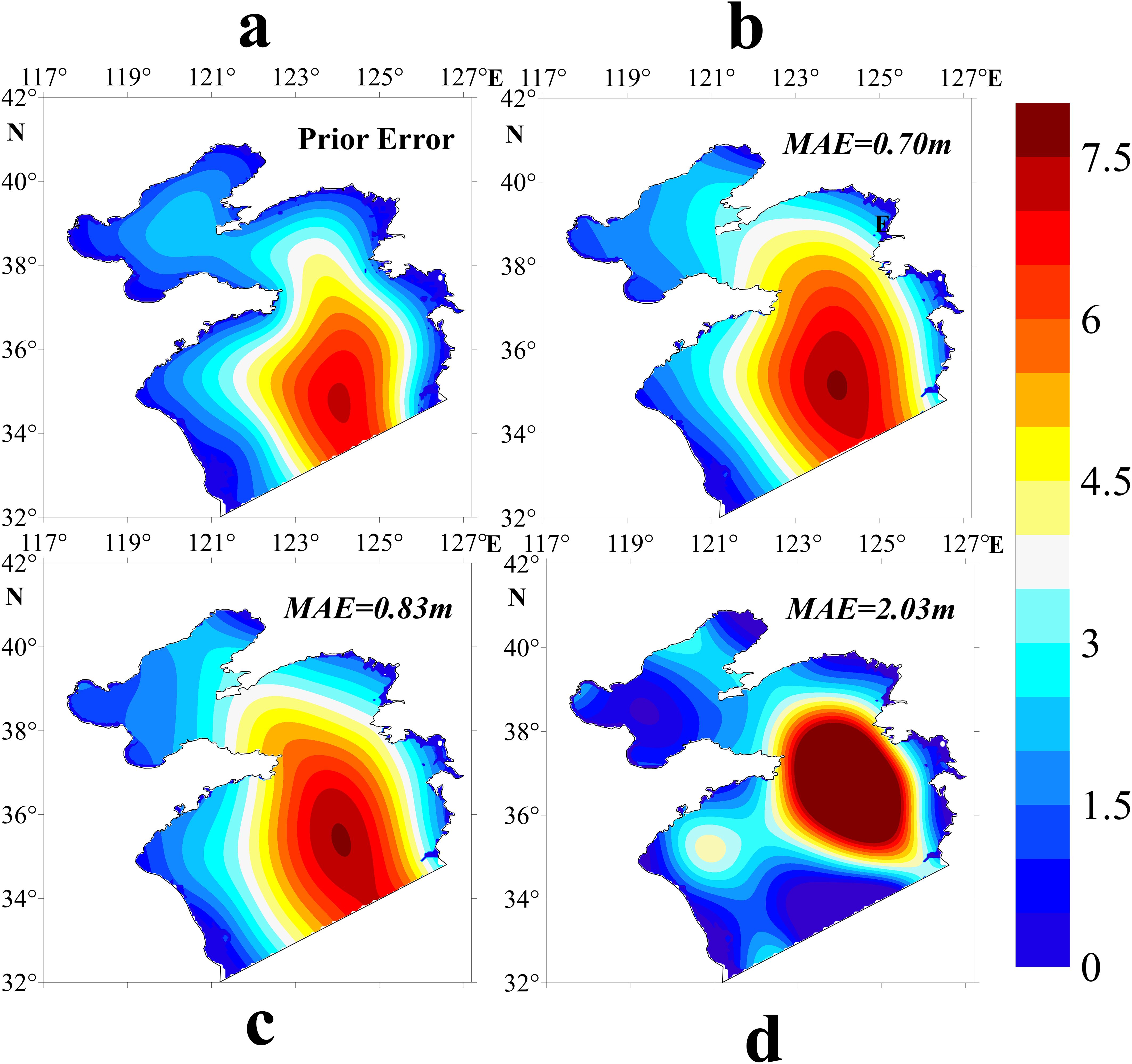
Figure 6. (A) The spatial distribution of prior bathymetry error (m), (B) the ensemble mean of $-\Delta H_n$, (C, D) are the ensemble member with the minimum MAE and the maximum MAE between- $-\Delta H_n$ and prior bathymetry error, respectively.

Conduct model integration using the BIPs ensemble after assimilation, and perform harmonic analysis based on the water levels from the ensemble mean to further evaluate the effects of bathymetry estimation. Table 1 lists the spatially averaged MAE and bias of harmonic constants. The bold font represents the smaller MAE or smaller absolute value of bias. It is easy to notice that all constituents improved except for the bias of Q₁ constituent. The prior spatially averaged bias of Q₁ is smaller than 0.001, which is due to the discrepancy of amphidromic points. The spatial averaging causes the large deviations near the amphidromic points. Coincidentally, the deviations canceled out the difference in other areas. As a result, the averaged bias becomes close to 0.

Table 1

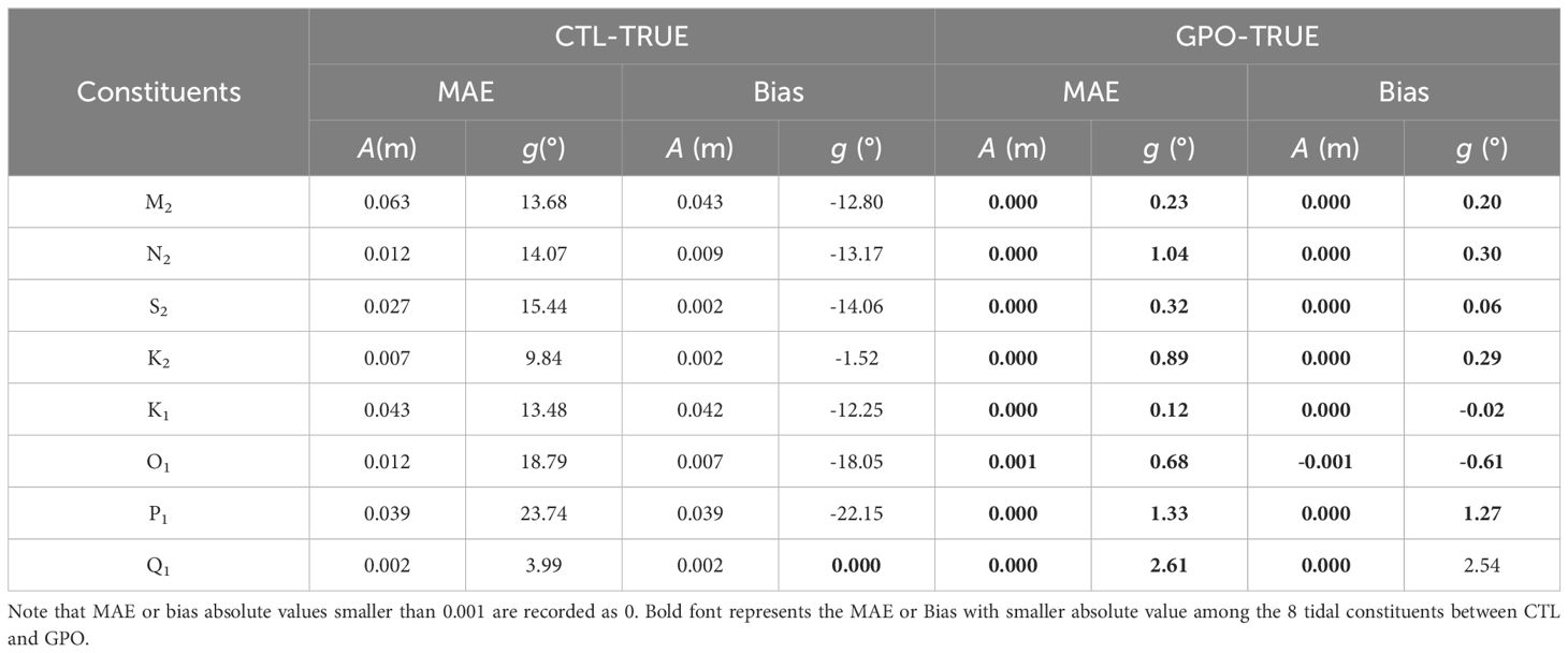
Table 1. Spatially averaged MAE and bias of amplitude ($A$) and phase lag ($g$) for each constituents CTL compared with “true” state.

5 Practical experiments based on NAO.99Jb

5.1 Experiments based on M₂ tide model

5.1.1 Experiment settings

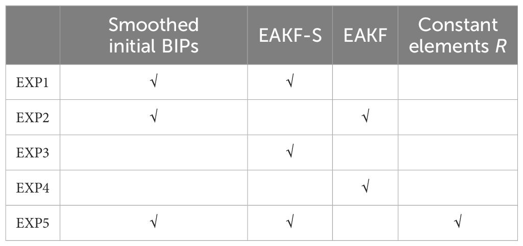
In this section, the BYM is simplified to consider only the M₂ constituent. The performance of EAKF-S in practical GPO experiments is discussed. The influence of the smoothing term and the confidence matrix (R) are explained through 5 experiments, which are listed in Table 2. Note that the $\text{λ}$ is set to 1 based on the results of a series of experiments. EXP1 — EXP5 are divided based on whether the initial BIPs are smoothed, whether EAKF-S or standard EAKF is applied, and whether a constant elements confidence matrix ($R$) is used. Note that the values of constant elements are all equal to the average of the spatially varying $\text{R}$.

Table 2

Table 2. Experiment settings of EXP1 — EXP5.

Following the duration of the experiment with the longest spin-up time (EXP4), the GPO experiments mentioned above are set to last 8 days. Since NAO.99Jb (1/12° of spatial resolution) can generate water level data for any time and location within the coverage area, to ensure consistency between the twin experiment and practical experiments, the observation resolution was set to hourly and 1/10°. The NAO.99Jb data of the M₂ constituent was used in this section. Due to the minimum bathymetry being set to 5 m, the BYM does not accurately represent the bathymetry in shallow regions. The simulation accuracy in these areas is expected to be relatively worse. Therefore, a standard deviation of observational error ${\text{σ}}^o$ strictly determined by the observational error leads to a high tendency of EAKF to prioritize optimizing these shallow areas with larger errors. Hence, to achieve a better and reasonable result, the ${\text{σ}}^o$ of the NAO.99Jb observations are specified regionally. For the $n$th observation, the ${\text{σ}}^o$ is given by the Equation 19 below:

$\begin{array}{ll}\{\begin{array}{cc}{\sigma }^o(n)=0.4m,\hfill & \hfill 5m\le H_{ETOPO5}(n)\le 20m\\ {\sigma }^o(n)=0.1m,\hfill & \hfill H_{ETOPO5}(n)>20m\\ {\sigma }^o(n)=0.8m,\hspace{1em}\hfill & \hfill {125.4}^{°}E<lon(n)<{127.0}^{°}E,{36.8}^{°}N<lat(n)<{38.0}^{°}N\end{array}& (19)\end{array}$

where $H_{ETOPO5}(n)$ is the ETOPO5 bathymetry of the observation; $lon$ and $lat$ represent the longitude and latitude of the observation, respectively. The region defined by $lon$ and $lat$ in the equation above is Ganghwa Bay, characterized by its extensive tidal flats. The resolution of the BYM (1/30°) makes it challenging to accurately represent the complex bathymetry of Ganghwa Bay. The accuracy of forecasting water levels is poor and difficult to optimize. With relatively small ${\sigma }^o$, the EAKF may become overly focused on optimizing water levels specifically within Ganghwa Bay, potentially leading to negative impacts on the overall optimization outcomes.

5.1.2 Results

Figure 7 shows the time series of spatially averaged prior water level RMSE for EXP1 — EXP5. Before the GPO started, the RMSE values for all experiments were very close. Whether the initial BIPs were smoothed or not didn’t significantly affect the overall precision of state estimation. Thus, all experiments had a relatively “fair” start for the GPO process. After the jointly state and parameter optimization was activated, the spin-up periods of GPO varied between EXP4 and the other experiments. Compared with EXP2, which shares the same GPO scheme, the spin-up time of EXP4 is notably longer. This indicates that the smoothed, continuous BIPs allow the EAKF to better capture the patterns of the spatial distribution. The accuracy of the observational increment projection to the parameter was then enhanced. However, as the EAKF progresses, the lack of spatial smoothing leads to the accumulation of small-scale errors in the ensemble. Consequently, the RMSE converges to a level similar to that of the unsmoothed initial BIPs. By comparison, with the EAKF-S, the RMSEs of EXP1 and EXP3 are significantly smaller than EXP2 and EXP4. The smoothing term substantially enhances the performance of the EAKF on GPO. It can be noticed that the RMSE of EXP1 is only slightly smaller than EXP3. After the GPO started, the BIP ensemble of EXP3 was smoothed during the first implementation of EAKF-S. In the end, there is little difference between EXP1 and EXP3. However, applying the smoothing term to the initial BIP ensemble carries only benefits and poses no harm. It helps prevent inaccurate estimation in the first GPO step and enhances the robustness of GPO based on EAKF.

Figure 7

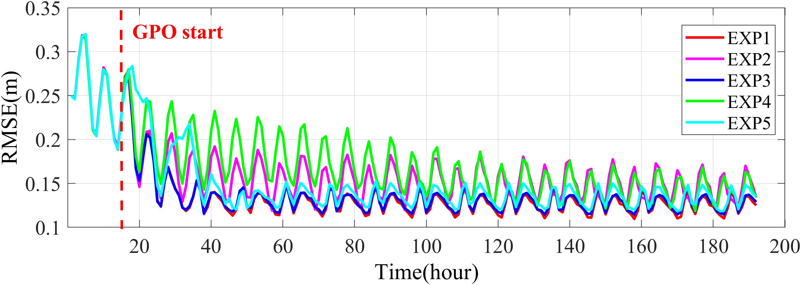
Figure 7. Time series of prior water level spatially averaged RMSE of EXP1—EXP5, the red dashed line represents the start time of GPO.

Compared to EXP1, the water level RMSE is only slightly worse in EXP5, yet the difference remains pronounced. Figure 8 shows a filled plot of the time series of water level MAE ensemble distribution, with the cyan shaded area representing EXP1 and the magenta shaded area the EXP5. Besides the larger RMSE, there is also marked variability in the distribution of the ensemble. During the spin-up phase, the ensemble spread of EXP5 was ranging from 9×10^-3 m to 0.09 m, which implies a mismatch between EAKF and the constant elements $R$. As mentioned above, the BIPs near the coast are much more sensitive than those in the central sea areas of Bohai Sea and Yellow Sea. Many of the BIPs were adjusted excessively by the smoothing term. The distribution of posterior BIPs was altered and deviated from the pattern formed by EAKF. With the continuous adjustment, due to the constraints of ${\text{P}}^b$, EAKF-S is still able to approximate the optimal BIPs that correspond to the water level errors. However, the mismatch between the covariance matrix ${\text{cov}}_{x,y}^p$ and the constant elements $\mathit{\text{R}}$ still results in weaker performance compared to EXP1. In other words, the EAKF is searching for the optimal BIP that satisfies both the smoothing term and the model correlations.

Figure 8

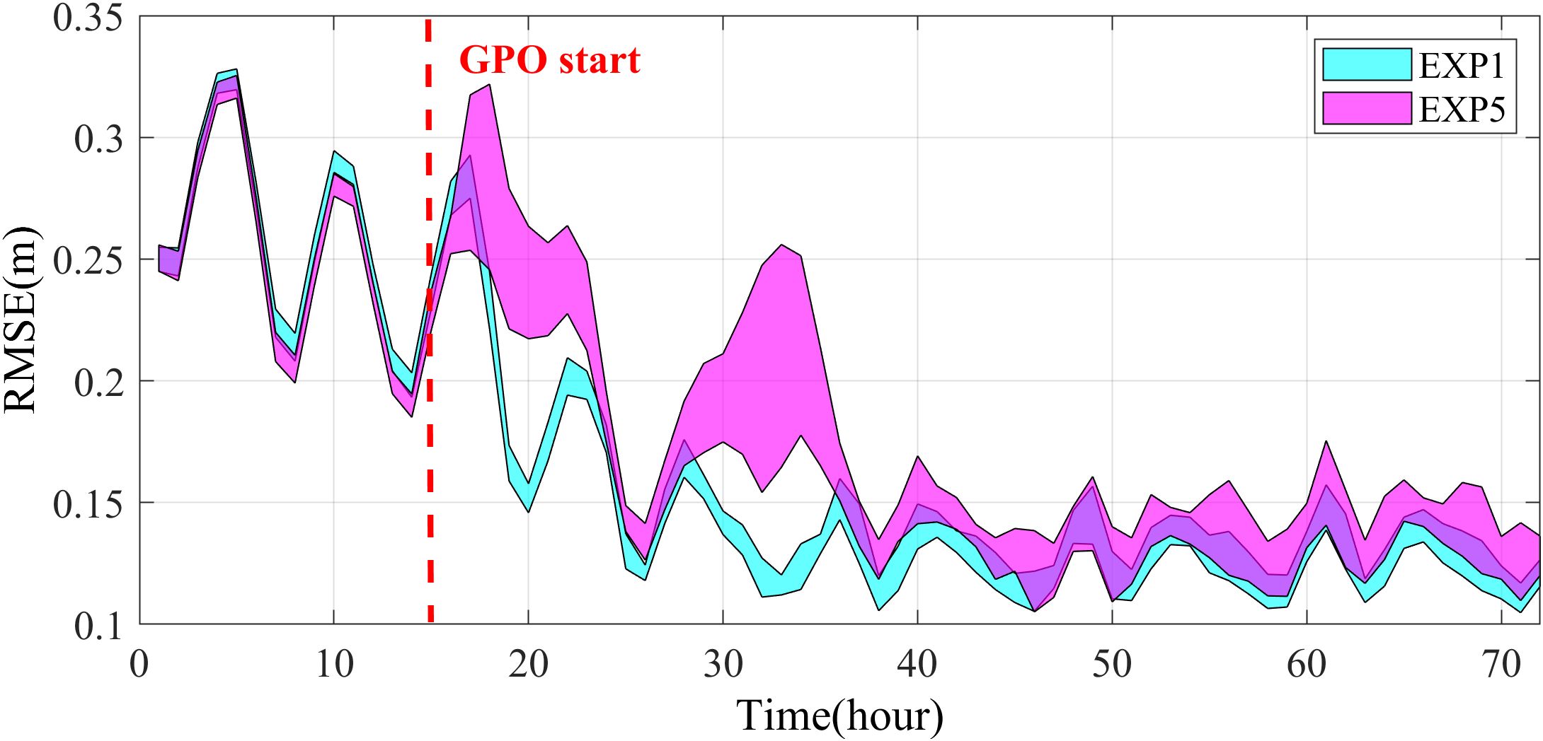
Figure 8. Time series of ensemble distribution of prior water level MAE for EXP1 (cyan) and EXP5 (magenta).

Figure 9 shows the differences in amplitudes and phase lags of the model before data assimilation (or the control model, CTL) and EXP1 compared to those of NAO.99Jb. As shown in the figure, EAKF-S notably improved the model harmonic constants. Compared to NAO.99Jb, the spatially averaged amplitude and phase lag errors of CTL are 0.25 m and 23.93°, respectively. For EXP1, these errors are 0.05 m and 3.59°, respectively. It can be observed that the amplitude and phase lag errors of CTL are significantly higher in coastal area. Additionally, there is a great discrepancy in the locations of the amphidromic points between CTL and NAO.99Jb. The spatial distribution of amplitude errors in Figure 9A exhibits a spreading pattern around the amphidromic points. Correspondingly, there is a great phase lag difference between CTL and NAO.99Jb in Figure 9C. Conversely, in Figures 9B, D, both the errors in harmonic constants and the locations of the amphidromic points are significantly improved. There is only slight displacement observed of the amphidromic points in the northern Bohai Sea. Although the Ganghwa Bay area shows some improvement after GPO, significant deviations still exist. This is attributed to the inherent limitations of the model in accurately representing the complex bathymetry of Ganghwa Bay. It can’t be solved solely by adjusting the bathymetry.

Figure 9

Figure 9. (A, C) are the differences of amplitudes (m) and phase lags (°) between CTL and NAO.99Jb, respectively. (B, D) are similar with (A, C) but for the differences between EXP1 and NAO.99Jb.

5.2 Practical experiment based on 8 constituents tide model

5.2.1 Experiment settings

In this section, the BYM, which incorporates 8 tidal constituents as introduced in Section 4 is employed. The hourly tide height of 8 tidal constituents NAO.99Jb is used as observations. Considering both the tide period of 8 constituents and computational cost, we set the GPO period as 30 days.

The BYM model with 8 tidal constituents closely represents the complete ocean model in terms of complexity. By testing the performance on the BYM with 8 constituents, the effectiveness of EAKF-S is further evaluated in strongly nonlinear, long-period ocean model. In this experiment, we still used the spatially varying $R$ and set $\text{λ}$ to 0.5.

5.2.2 Results

Figure 10 presents the time series of the prior water level RMSE for the CTL, SEO, and GPO. As shown in the figure, the GPO performs significantly better than the others. The time-averaged RMSEs for the CTL, SEO, and GPO experiments are 0.31 m, 0.23 m, and 0.15 m, respectively. Furthermore, the RMSE curves for SEO and GPO differ in amplitude and period compared to CTL. On semi-diurnal and diurnal scales, the RMSE amplitude for GPO is also notably smaller than that of CTL and SEO. That indicates the EAKF can capture the overall tidal patterns. Generally, EAKF-S demonstrates a considerable improvement in model accuracy.

Figure 10

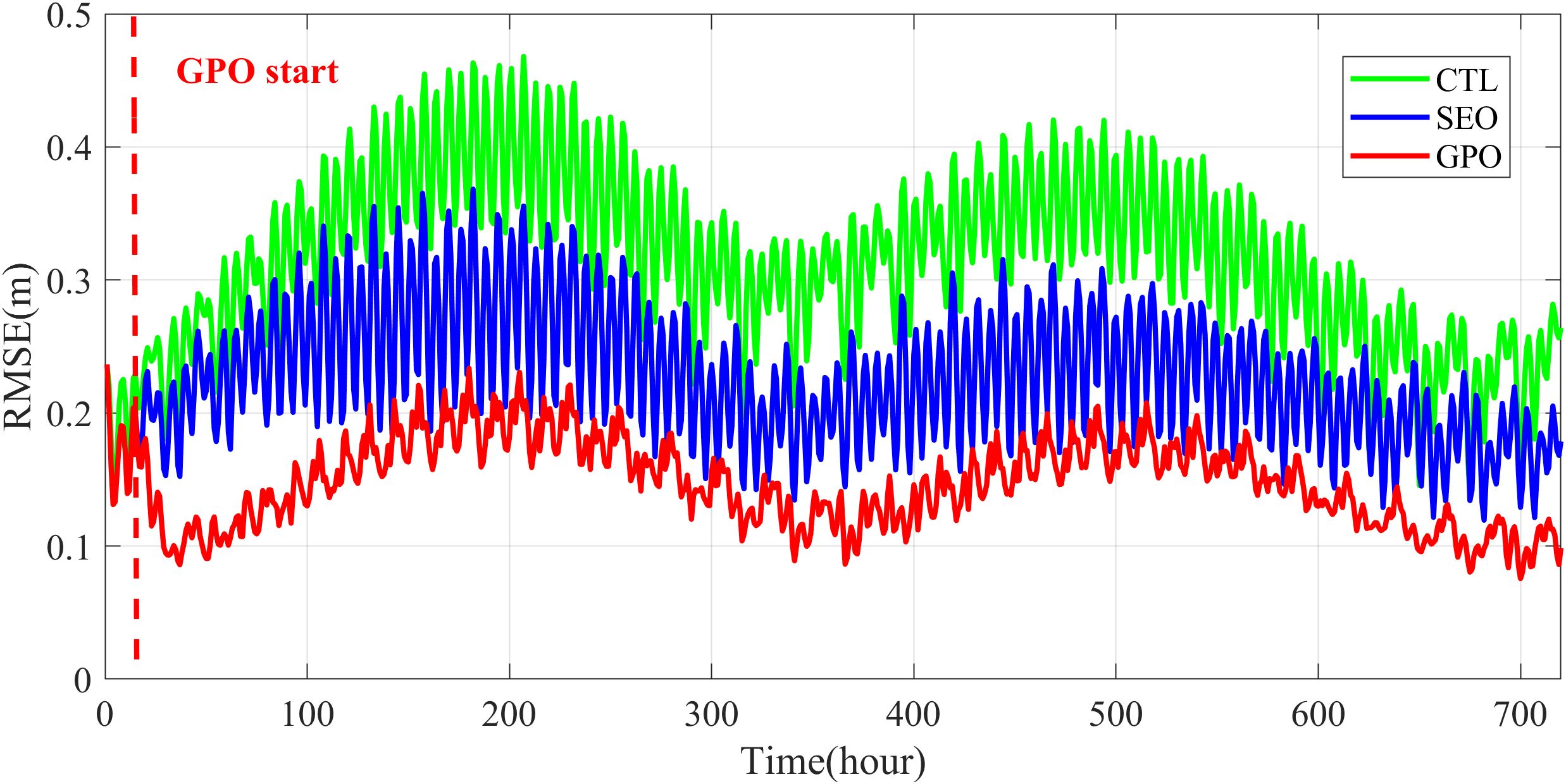
Figure 10. Time series of prior water level RMSE of CTL (green line), SEO (blue line) and GPO (red line).

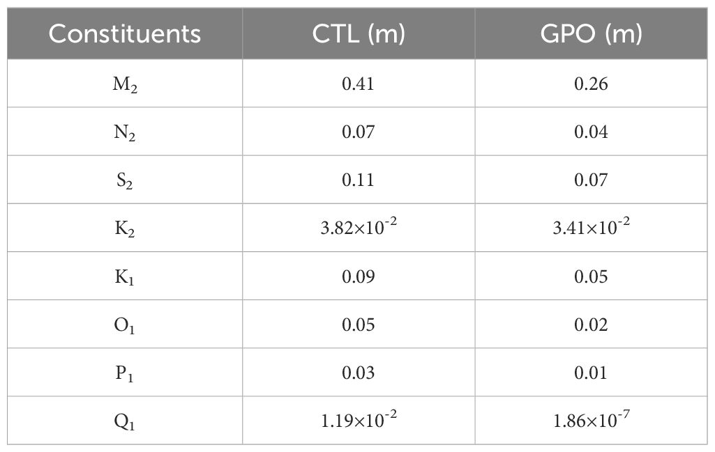
To assess the improvement of harmonic constants, we define the vectorial error $d$ (Fang et al., 2004) between the NAO.99Jb and GPO or CTL for each constituent. The amplitude is represented as the magnitude and the phase lag as the angle:

$\begin{array}{ll}d=\sqrt{A^2+A_{NAO}^2-2A{A}_{NAO}\cos (ɡ-{ɡ}_{NAO})},& (20)\end{array}$

where $A$ and $ɡ$ are the amplitude and phase lag from CTL or GPO, respectively; $A_{NAO}$ and ${ɡ}_{NAO}$ are the amplitude and phase lag from NAO.99Jb.

Table 3 lists the spatially averaged $d$ of CTL and GPO. For all 8 constituents, the $d$ for GPO are smaller than CTL, demonstrating the comprehensive improvement of water level after assimilation.

Table 3

Table 3. Vectorial errors ($d$) of harmonic constants from CTL and GPO compared with NAO.99Jb.

As shown in Figures 11, 12, there are great improvements in the amplitude and phase lag at the coastal area compared to CTL. Two main factors can be attributed. First, the amplitude near the coast is larger, resulting in greater error between the model and observations. Greater weights are given to those grid points in EAKF-S. Second, the BIPs are more sensitive in shallow areas. The EAKF favors optimizing these highly sensitive parameters due to the larger covariance values. For example, the region with the largest amplitude within the computational domain is Ganghwa Bay. Despite being assigned a large observation error, the EAKF still recognizes that improving Ganghwa Bay can efficiently enhance the overall model accuracy. The harmonic constants for all constituents in this region have improved after assimilation. Additionally, the Q₁ constituent shows the poorest spatial pattern of amplitude and phase lag errors. This is because NAO.99Jb has two amphidromic points in the Bohai Sea, while CTL has only one. The distinct tidal patterns between the BYM and NAO.99Jb result in a great difficulty of tuning the Q₁ constituent. Furthermore, the Q₁ constituent contributes minimally to water level deviations, with the maximum amplitude of the Q₁ constituent being only 0.05 m in NAO.99Jb. Thus, EAKF-S is unable to effectively improve the location and number of the amphidromic points of Q₁ constituent.

Figure 11

Figure 11. he amplitude differences (m) of M₂ (A, B), N₂ (C, D), S₂ (E, F), K₂ (G, H), K₁ (I, J), O₁ (K, L), P₁ (M, N), Q₁ (O, P) constituents of CTL and GPO compared with NAO.99Jb, respectively.

Figure 12

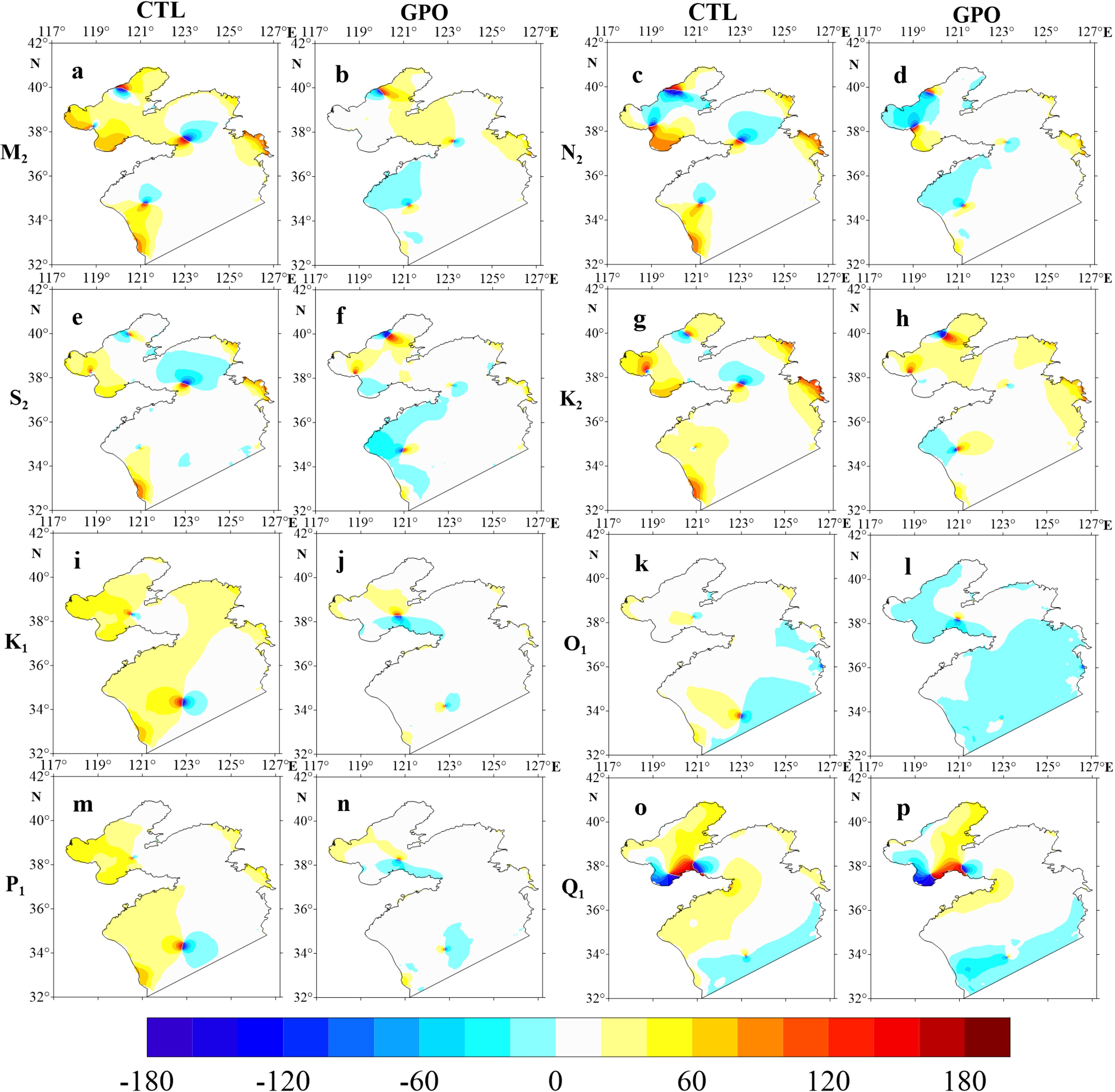
Figure 12. The phase lag differences (°) of M₂ (A, B), N₂ (C, D), S₂ (E, F), K₂ (G, H), K₁ (I, J), O₁ (K, L), P₁ (M, N), Q₁ (O, P) constituents of CTL and GPO compared with NAO.99Jb, respectively.

6 Conclusions and discussion

A full-grid parameter optimization scheme based on the EAKF, referred to as the EAKF-S, was proposed. By smoothing the ensemble members after the standard EAKF process, the correlation between parameters and state variables are simplified, enabling optimization with a limited ensemble size. A numerical tide model for the Bohai and Yellow Seas (BYM) was constructed using POMgcs. The feasibility of EAKF-S was discussed through twin experiment for bathymetry estimation of the 8 tide constituents’ model. Practical experiments using the NAO.99Jb data were also performed to examine the effectiveness and reliability of EAKF-S.

Twin experiment for full-grid bathymetry estimation were conducted under a “perfect model” scenario — the “true” model can be fully achieved by adjusting the parameters to be estimated. Results show that EAKF-S not only effectively reduces model state errors but also accurately inverts the true bathymetry. The plausible optimized parameter distribution thoroughly demonstrates the effectiveness of the scheme.

Further practical GPO experiments revealed that the smoothing term implicitly introduces spatial correlation of parameters while filtering out small-scale error signals. Under a comparable error level, using the EAKF-S scheme improved the accuracy of the GPO and reduced the spin-up time of the EAKF. The experiments also indicate that the current smoothing term still introduces inaccurate correlations between parameters and state. The confidence matrix $R$ based on sensitivity performs better than the constant elements. However, the $\text{R}$ used in this study remains overly simplified, warranting further exploration of this issue.

The EAKF-S scheme was applied to the BYM with 8 tide constituents and still effective in improving forecasting performance. Despite promising results, challenges remain. In this study, only single-parameter GPO was conducted. To achieve global optimization results and eliminate the issue of pseudo-correlations caused by adjusting bathymetry only, it is necessary to consider open boundary conditions and bottom friction coefficient to conduct multi-parameter optimization. On the other hand, the NAO.99Jb data used in this study consist of tide heights with globally consistent spatial scale and accuracy. Exploring the optimization performance of EAKF-S under multi-source and discrete observations will be a focus of future research.

Data availability statement

The datasets presented in this study can be found in online repositories (Wu et al., 2024). The names of the repository/repositories and accession number(s) can be found in the article/Supplementary Material.

Author contributions

HW: Conceptualization, Formal analysis, Methodology, Software, Visualization, Writing – original draft. WL: Conceptualization, Funding acquisition, Methodology, Project administration, Supervision, Validation, Writing – review & editing. GH: Conceptualization, Funding acquisition, Project administration, Supervision, Validation, Writing – review & editing. LC: Conceptualization, Methodology, Validation, Writing – review & editing. XC: Resources, Software, Writing – review & editing. KL: Methodology, Software, Writing – review & editing. GZ: Validation, Writing – review & editing, Visualization. QZ: Writing – review & editing, Visualization.

Funding

The author(s) declare financial support was received for the research, authorship, and/or publication of this article. This research is cosponsored by grants from the National Key Research and Development Program (2023YFC3107800) and the National Natural Science Foundation (42376190 and 41876014) of China.

Acknowledgments

The authors acknowledge valuable discussions with Xiaobo Wu from the National Marine Environmental Forecasting Center, Beijing China.

Conflict of interest

The authors declare that the research was conducted in the absence of any commercial or financial relationships that could be construed as a potential conflict of interest.

Publisher’s note

All claims expressed in this article are solely those of the authors and do not necessarily represent those of their affiliated organizations, or those of the publisher, the editors and the reviewers. Any product that may be evaluated in this article, or claim that may be made by its manufacturer, is not guaranteed or endorsed by the publisher.

Supplementary material

The Supplementary Material for this article can be found online at: https://www.frontiersin.org/articles/10.3389/fmars.2024.1479335/full#supplementary-material

References

Aksoy A., Zhang F., Nielsen-Gammon J. W. (2006). Ensemble-based simultaneous state and parameter estimation with MM5. Geophysical Res. Lett. 33, L12801. doi: 10.1029/2006GL026186

Crossref Full Text | Google Scholar

Anderson J. L. (2001). An ensemble adjustment Kalman filter for data assimilation. Monthly Weather Rev. 129, 2884—2903. doi: 10.1175/1520-0493(2001)129<2884:AEAKFF>2.0.CO;2

Crossref Full Text | Google Scholar

Anderson J. L. (2003). A local least squares framework for ensemble filtering. Monthly Weather Rev. 131, 634—642. doi: 10.1175/1520-0493(2003)131<0634:ALLSFF>2.0.CO;2

Crossref Full Text | Google Scholar

Anderson J. L., Anderson S. L. (2001). A Monte Carlo implementation of the nonlinear filtering problem to produce ensemble assimilations and forecasts. Monthly Weather Rev. 127, 2741–2758. doi: 10.1175/1520-0493(1999)127<2741:AMCIOT>2.0.CO;2

Crossref Full Text | Google Scholar

Blumberg A. F., Mellor G. L. (1987). A description of a three-dimensional coastal ocean circulation model, in Three-dimensional coastal ocean modelsvol. 4Ed. (Coastal and Estuarine Sciences), 1–16. doi: 10.1029/CO004p0001

Crossref Full Text | Google Scholar

Courant R., Friedrichs K., Lewy H. (1967). On the partial difference equations of mathematical physics. J. Res. Dev. 11, 215—234. doi: 10.1147/rd.112.0215

Crossref Full Text | Google Scholar

Courtier P., Talagrand O. (1987). Variational assimilation of meteorological observations with the adjoint vorticity equation II: Numerical results. Q. J. R. Meteorological Soc. 113, 1329—1347. doi: 10.1002/qj.49711347813

Crossref Full Text | Google Scholar

Das S. K., Lardner R. W. (1991). On the estimation of parameters of hydraulic models by assimilation of periodic tidal data. J. Geophys. Res. Oceans 96, 15187–15196. doi: 10.1029/91JC01318

Crossref Full Text | Google Scholar

Evensen G. (1994). Sequential data assimilation with a nonlinear quasi geostrophic model using Monte-Carlo methods to forecast error statistics. J. Geophysical Research: Oceans 99, 10143—10162. doi: 10.1029/94JC00572

Crossref Full Text | Google Scholar

Evensen G. (2004). Sampling strategies and square root analysis schemes for the EnKF. Ocean Dynamics 54, 539—560. doi: 10.1007/s10236-004-0099-2

Crossref Full Text | Google Scholar

Ezer T., Mellor G. L. (2004). A generalized coordinate ocean model and a comparison of the bottom boundary layer dynamics in terrain-following and in z-level grids. Ocean Modelling. 6, 379—403. doi: 10.1016/S1463-5003(03)00026-X

Crossref Full Text | Google Scholar

Fan R., Zhao L., Lu Y., Nie H., Wei H. (2019). Impacts of currents and waves on bottom drag coefficient in the East China shelf seas. J. Geophysical Research: Oceans 124, 7344—7354. doi: 10.1029/2019jc015097

Crossref Full Text | Google Scholar

Fang G., Wang Y., Wei Z., Choi B. H., Wang X., Wang J. (2004). Empirical cotidal charts of the Bohai, Yellow, and East China Seas from 10 years of TOPEX/Poseidon altimetry. J. Geophysical Research: Oceans 109, C11006. doi: 10.1029/2004jc002484

Crossref Full Text | Google Scholar

Gaspari G., Cohn S. E. (1999). ). Construction of correlation functions in two and three dimensions. Q. J. R. Meteorological Soc. 125, 723—757. doi: 10.1002/qj.49712555417

Crossref Full Text | Google Scholar

Guo Z., Pan H., Fan W., Lv X. (2017). Application of surface spline interpolation in inversion of bottom friction coefficients. J. Atmospheric Oceanic Technol. 34, 2021—2028. doi: 10.1175/JTECH-D-17-0012.1

Crossref Full Text | Google Scholar

Han G., Li W., He Z., Liu K., Ma J. (2006). Assimilated tidal results of tide gauge and TOPEX/POSEIDON data over the China seas using a variational adjoint approach with a nonlinear numerical model. Adv. Atmospheric Sci. 23, 449—460. doi: 10.1007/s00376-006-044908

Crossref Full Text | Google Scholar

Heemink A. W., Mouthaan E. E. A., Roest M. R. T., Vollebregt E. A. H., Robaczewska K. B., Verlaan M. (2002). Inverse 3D shallow water flow modelling of the continental shelf. Continental Shelf Res. 22, 465—484. doi: 10.1016/S0278-4343(01)00071-1

Crossref Full Text | Google Scholar

Lardner R. W., Al-Rabeh A. H., Gunay N. (1993). Optimal estimation of parameters for a two-dimensional hydrodynamical model of the Arabian Gulf. J. Geophysical Research: Oceans 98, 18229. doi: 10.1029/93JC01411

Crossref Full Text | Google Scholar

Li Z., Peng Z., Zhang Z., Chu Y., Xu C., Yao S., et al. (2023). Exploring modern bathymetry: A comprehensive review of data acquisition devices, model accuracy, and interpolation techniques for enhanced underwater mapping. Front. Mar. Sci. 10, 1178845. doi: 10.3389/fmars.2023.1178845

Crossref Full Text | Google Scholar

Li W., Xie Y., Han G. (2013). A theoretical study of the multigrid three-dimensional variational data assimilation scheme using a simple bilinear interpolation algorithm. Acta Oceanologica Sin. 32, 80—87. doi: 10.1007/s13131-013-0292-6

Crossref Full Text | Google Scholar

Li W., Xie Y., He Z., Han G., Liu K., Ma J., et al. (2008). Application of the multigrid data assimilation scheme to the China sea’s temperature forecast. J. Atmospheric Oceanic Technol. 25, 2106—2116. doi: 10.1175/2008JTECHO510.1

Crossref Full Text | Google Scholar

Liang K., Li W., Han G., Wang X., Qiu X. (2023). An operational improvement of A-4DEnVar and its application to the estimation of the spatially varying bottom friction coefficients of the M₂ constituent in the Bohai and Yellow seas. Front. Mar. Sci. 9. doi: 10.3389/fmars.2022.1084159

Crossref Full Text | Google Scholar

Matsumoto K., Takanezawa T., Ooe M. (2000). Ocean tide models developed by assimilating TOPEX/POSEIDON altimeter data into hydrodynamical model: A global model and a regional model around Japan. J. Oceanography 56, 567—581. doi: 10.1023/A:1011157212596

Crossref Full Text | Google Scholar

Panchang V. G., O’Brien J. J. (1989). “On the determination of hydraulic model parameters using the adjoint state formulation,” in .), modelling marine system. Ed. Davis A. M. (CRC Press, Boca Raton, FL), 6—18.

Google Scholar

Rabier F., Järvinen H., Klinker E., Mahfouf J. F., Simmons A. (2000). The ECMWF operational implementation of four-dimensional variational assimilation. I: Experimental results with simplified physics. Q. J. R. Meteorological Soc. 126, 1143—1170. doi: 10.1002/qj.49712656415

Crossref Full Text | Google Scholar

Smedstad O. M., O’Brien J. J. (1991). Variational data assimilation and parameter estimation in an equatorial Pacific Ocean model. Prog. Oceanography 26, 179—241. doi: 10.1016/0079-6611(91)90002-4

Crossref Full Text | Google Scholar

Stammer D., Wunsch C., Giering R., Eckert C., Heimbach P., Marotzke J., et al. (2002). Global ocean circulation during 1992–1997, estimated from ocean observations and a general circulation model. J. Geophysical Research: Oceans 107, 3118. doi: 10.1029/2001JC000888

Crossref Full Text | Google Scholar

Talagrand O., Courtier P. (1987). Variational assimilation of meteorological observations with the adjoint vorticity equation. I: Theory. Q. J. R. Meteorological Soc. 113, 1311—1328. doi: 10.1002/qj.49711347812

Crossref Full Text | Google Scholar

Tippett M. K., Anderson J. L., Bishop C. H., Hamill T. M., Whitaker J. S. (2003). Ensemble square root filters. Monthly Weather Rev. 131, 1485—1490. doi: 10.1175/1520-0493(2003)131<1485:ESRF>2.0.CO;2

Crossref Full Text | Google Scholar

Tong M., Xue M. (2008). Simultaneous estimation of microphysical parameters and atmospheric state with simulated radar data and ensemble square root Kalman filter. Part II: parameter optimization experiments. Monthly Weather Rev. 136, 1649—1668. doi: 10.1175/2007MWR2070.1

Crossref Full Text | Google Scholar

Wilson G., Özkan-Haller H. T. (2012). Ensemble-based data assimilation for estimation of river depths. J. Atmospheric Oceanic Technol. 29, 1558—1568. doi: 10.1175/JTECH-D-12-00014.1

Crossref Full Text | Google Scholar

Wilson G., Özkan-Haller H. T., Holman R. (2010). Data assimilation and bathymetric inversion in a two-dimensional horizontal surf zone model. J. Geophysical Research: Oceans 115, C12057. doi: 10.1029/2010JC006286

Crossref Full Text | Google Scholar

Wilson G., Özkan-Haller H. T., Holman R., Haller M. C., Honegger D. A., Chickadel C. C. (2014). Surf zone bathymetry and circulation predictions via data assimilation of remote sensing observations. J. Geophysical Research: Oceans 119, 1993—2016. doi: 10.1002/2013JC009213

Crossref Full Text | Google Scholar

Wu H., Li W., Han G., Cao L., Cui X., Liang K., et al. (2024). Full-grid bathymetry estimation in the numerical simulation of 8 tidal constituents using an ensemble adjustment Kalman filter-smoothing scheme [Dataset. Figshare. doi: 10.6084/m9.figshare.26343856

Crossref Full Text | Google Scholar

Wu X., Zhang S., Liu Z., Rosati A., Delworth T. L., Liu Y. (2012). Impact of geographic-dependent parameter optimization on climate estimation and prediction: simulation with an intermediate coupled model. Monthly Weather Rev. 140, 3956—3971. doi: 10.1175/MWR-D-11-00298.1

Crossref Full Text | Google Scholar

Zhang S., Anderson J. ,. L., Rosati A., Harrison M. ,. J., Khare S. P., Wittenberg A. (2004). Multiple time level adjustment for data assimilation. Tellus 56A, 2—15. doi: 10.1111/j.1600-0870.2004.00040.x

Crossref Full Text | Google Scholar

Zhang S., Liu Z., Rosati A., Delworth T. (2012). A study of enhancive parameter correction with coupled data assimilation for climate estimation and prediction using a simple coupled model. Tellus 64A, 10963. doi: 10.3402/tellusa.v64i0.10963

Crossref Full Text | Google Scholar

Zhang J. C., Lu X. Q. (2008). Parameter optimization for a three-dimensional numerical barotropic tidal model with adjoint method. Numerical Methods Fluids 57, 47—92. doi: 10.1002/fld.1620

Crossref Full Text | Google Scholar

Zhang J. C., Lu X. Q., Wang P., Wang Y. P. (2011). Study on linear and nonlinear bottom friction parameterizations for regional tidal models using data assimilation. Continental Shelf Res. 6, 555—573. doi: 10.1016/j.csr.2010.12.011

Crossref Full Text | Google Scholar