Wind-driven nearshore overturning currents off the northeastern Shandong Peninsula in the Yellow Sea in winter

Introduction: The nearshore sea off the northeastern Shandong Peninsula is characterized by intensive mariculture, whose ecosystem is involved in the large marine ecosystem of the Yellow Sea. However, ocean currents in this area are poorly explored. Observations suggested overturning currents were robust phenomena in winter in this area.

Methods: Numerical simulations and experiments were used to investigate the mechanisms of overturning currents.

Results: There were two classes of wind-driven overturning currents. One consisted of surface southeastward currents, nearshore downwelling currents, and bottom northeastward currents. The other consisted of surface northeastward currents, nearshore upwelling currents, and bottom southwestward currents.

Discussion: The underlying dynamics involved local wind forcing and propagation of coastal trapped waves (CTWs). Northwesterly winds in the Bohai Sea and North Yellow Sea drove surface southward currents and converged water toward coastline off the northeastern Shandong Peninsula, generating nearshore sea level rising. The resultant southward sea level slope drove nearshore bottom northward currents. Meanwhile, high sea level in the southern part of Bohai Sea and North Yellow Sea also propagated as CTWs clockwise around the Shandong Peninsula, which further enhanced nearshore bottom northward currents and caused eastward currents in the entire water column off the northeastern Shandong Peninsula. Southwesterly winds in the Bohai Sea and North Yellow Sea drove surface northward currents, generating nearshore sea level dropping off the northeastern Shandong Peninsula. The resultant northward sea level slope caused bottom southward currents. Meanwhile, the southwesterly winds caused CTWs with low sea level in the south part of the Bohai Sea and Yellow Sea. The northward sea level slope of CTWs enhanced nearshore bottom southwestward currents. The current study emphasized winds in winter drove not only local currents but also propagation of CTWs in the Bohai Sea and North Yellow Sea. The sea level slope of CTWs regulated surface and bottom Ekman layers driven by local winds.

1 Introduction

Wind-driven currents are a common phenomenon in the nearshore sea with shallow waters. Previous studies have shown that along-shelf and cross-shelf winds generate nearshore overturning currents (Austin and Lentz, 2002; Tilburg, 2003). When downwelling-favorite winds prevail, onshore currents occur at sea surface with water converged in the nearshore area. This results in nearshore sea level rising and downwelling currents. Nearshore high sea level drives bottom offshore currents. When upwelling-favorite winds prevail, there are surface offshore currents, bottom onshore currents, and nearshore upwelling currents with nearshore low sea level. The aforementioned wind-driven overturning currents result in vertical displacements and cross-shelf exchange (Austin and Lentz, 2002; Tilburg, 2003; Lentz and Fewings, 2011; Kämpf, 2017). The cross-shelf exchange of water masses is important for transporting nutrients and low-oxygen water masses between the shore and the open ocean (Garland et al., 2002; Grantham et al., 2004; Lentz and Fewings, 2011).

As one of the important shelf seas of the western Pacific Ocean, the Yellow Sea is located between the northern China and the Korean Peninsula, connecting with the Bohai Sea to the northwest and the East China Sea to the south (Figure 1A). It has an average depth of approximately 44 m, with a deep trough in the central area extending northward to the Bohai Sea. Each year a large amount of freshwater and high nutrient loads from China and the Korean Peninsula are carried into the Bohai Sea and Yellow Sea by rivers, atmospheric depositions, wastewater discharges, and mariculture (Wang et al., 2003, 2019; Zhai et al., 2021a; Wu et al., 2023a). This results in a thriving marine ecosystem in the Yellow Sea, which is one of the most important large marine ecosystems in the world and makes great contributions to the socioeconomic development of China, North Korea, and South Korea (Zhang et al., 2019; Zhai et al., 2020a).

Figure 1

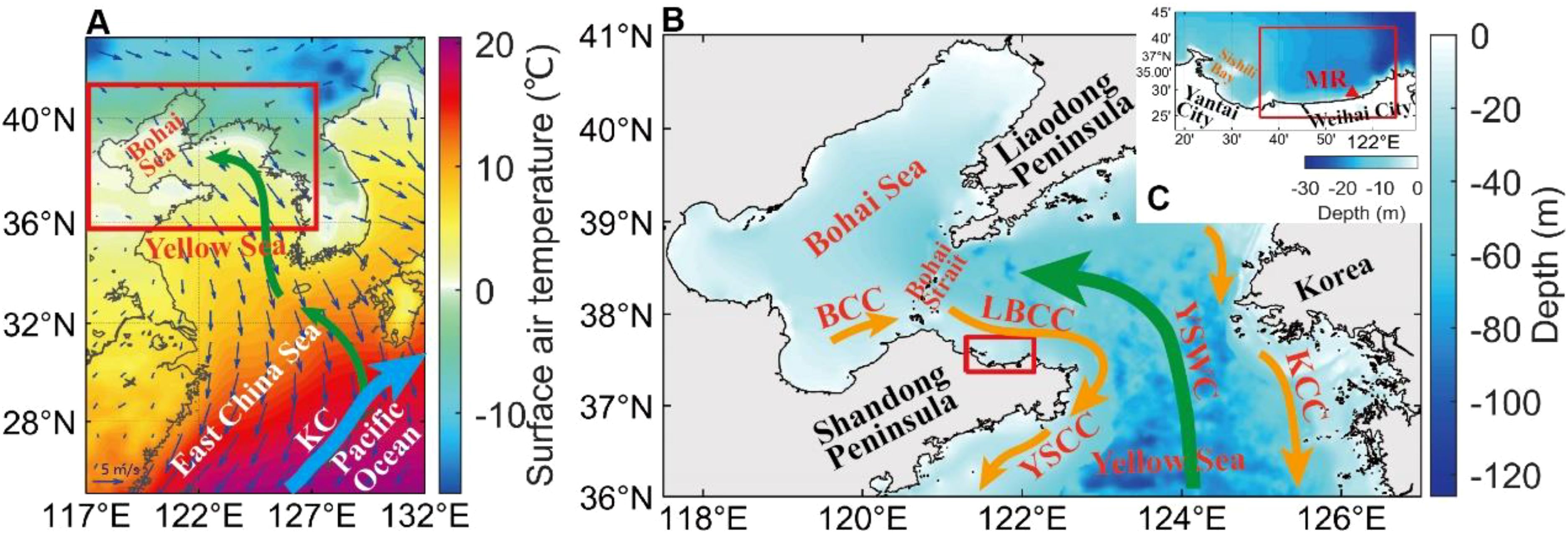
Figure 1. (A) Climatological winter mean 2-m air temperature (°C; color) and 10-m wind vectors (m s⁻¹; arrows) over the East Asia and adjacent seas. The red rectangle denotes the model domain in the current study. (B) Water depth (m) of the model domain in Bohai Sea and Yellow Sea. The red rectangle denotes the northeastern coastal oceans of the Shandong Peninsula. (C) Water depth (m) in northeastern coastal oceans of the Shandong Peninsula. The magenta rectangle denotes the study area east of the Yangma Island in this paper. The red triangle marks the submarine cable real-time observation site in the Yutai marine ranching area (MR). Thick arrows in (A, B) denote major currents in the East China Sea, Yellow Sea and Bohai Sea in winter: Kuroshio Current (KC), Yellow Sea Warm Current (YSWC), Yellow Sea Coastal Current (YSCC), Korean Coastal Current (KCC), Lubei Coastal Current (LBCC) and Bohai Coastal Current (BCC).

Ocean currents and water masses in the Yellow Sea are predominantly forced by the East Asian Monsoon system, land-sourced river runoffs, and Kuroshio Current originating from the large-scale circulation in the Pacific Ocean (Qu et al., 1999; Su, 2001; Zhai and Hu, 2013; Zhai et al., 2014). The spatiotemporal variations in the large-scale ocean circulation in the Yellow Sea have been well established by previous studies (Su, 2001). In winter, prevailing northerly/northwesterly monsoon winds form and maintain southward cold currents in coastal oceans, such as the Lubei Coastal Current, Yellow Sea Coastal Current, and Korean Coastal Current. Consequently, the Yellow Sea Warm Current (YSWC) in the central area occurs as a compensation (Figure 1; Su, 2001). Waters are mixed well from surface to bottom in the majority of the Yellow Sea. Significant thermocline subsequently develops in spring, peaks in summer, and decays in autumn. In summer, the Yellow Sea features a strong thermocline and a large volume of cold water in the deep layer of the central area (Zhang et al., 2008; Li et al., 2024). In the current study, seasons are those for the Northern Hemisphere, with winter referring to December-February, spring referring to March-May, summer referring to June-August, and autumn referring to September-November.

In winter, strong northerly monsoon drives YSWC in the central area of the Yellow Sea and Lubei Coastal Current (LBCC) off the northeastern Shandong Peninsula. One of the mechanisms of YSWC is the wind-driven barotropic current in the basin with a trough. Csanady (1973) developed wind forcing barotropic model with arbitrary topography and long basin to study circulations in similar bathymetries. Wind-driven barotropic models propose that YSWC is upwind current (Hsueh and Pang, 1989; Takahashi et al., 1995; Lin and Yang, 2011). In all models, there are currents downwind in shallow areas and upwind in deep trough (Csanady, 1973; Hsueh and Pang, 1989; Takahashi et al., 1995; Lin and Yang, 2011). The upwind currents last only for a few days as the two gyres evolve and propagate as topographic waves (Lin and Yang, 2011). Observations also confirm the circulations (Hsueh, 1988; Lin et al., 2011; Qu et al., 2018). Winds in the Bohai Sea and North Yellow Sea in winter show very strong synoptic variations in the north‐south direction with a period of less than one week, generating CTWs (Hsueh and Pang, 1989; Li and Huang, 2019). CTWs in the north Yellow Sea moved clockwise around the Shandong Peninsula (Hsueh and Pang, 1989; Li and Huang, 2019). Kelvin wave is the dominated component of CTWs in the Yellow Sea (Hsueh and Pang, 1989; Li and Huang, 2019). Meanwhile, the sea level slope of CTWs generates currents energetic with periods of 2–5 days (Li and Huang, 2019). The currents are in quasi-geostrophic balance with the cross-shelf pressure gradient (Wang et al., 2020). One branch of YSWC flows into Bohai and turns anticlockwise, then flows eastward off the northeastern Shandong Peninsula (Su and Yuan, 2005). Zheng et al. (2021) indicate that LBCC increases with the increasing northerly wind, and barotropic pressure gradient is the dominant driving force.

Spatiotemporal variations in the three-dimensional nearshore circulation in the Yellow Sea are still poorly understood. Note that nearshore waters of the Yellow Sea are with intensive mariculture and marine ranching, which are greatly influenced by both large-scale and regional ocean circulation systems (Zhai et al., 2021b; Wu et al., 2023b). Among them, the northeastern nearshore waters of the Shandong Peninsula are mainly farmed for precious seafood, such as sea cucumbers, abalones, and scallops, which are less mobile and therefore are more vulnerable to changes in ocean currents and water masses (Zhai et al., 2020a). Recently, submarine cable real-time observations indicated that there were possibly overturning currents in the northeastern nearshore waters of the Shandong Peninsula in winter (magenta rectangle in Figure 1C; Hu et al., 2021). Strong overturning currents could further affect the winter thermal structure and thus seasonal changes of the marine ecosystem in the marine ranching areas (Zhai et al., 2021c).

Based on high-resolution numerical simulations and experiments, the current study aimed to document the spatiotemporal variations in nearshore overturning currents off the northeastern Shandong Peninsula and clarify the underlying dynamics. The current study enriches the nearshore hydrodynamics and is helpful for further studies and predictions of the nearshore marine ecosystem. The rest of the paper is structured as follows: Section 2 describes the data, numerical model, and methods. Section 3 presents the characteristics of wind-driven overturning currents by composite analysis. In section 4, the primarily impact factors of currents in all events are firstly researched. Then dynamics in the typical events are investigated. Idealized conceptual experiments were used to illustrate that the dynamic processes are the primary and robust processes, even though winds were changed. Section 5 gives a summary of the current study.

2 Observations, numerical model and methodology

2.1 Observations

As shown by the magenta rectangle in Figure 1C, the study area is located to the east of Sishili Bay in the northeastern coastal waters of the Shandong Peninsula. In this region, the topography is basically flat in most offshore areas with water depth being approximately 20.0 m and is sloping approaching the shoreline. The shoreline is roughly zonal. To better understand current variations in the northeastern nearshore waters of the Shandong Peninsula, we used observations obtained from the submarine cable real-time observation system (SCROS) in the Yutai marine ranching area (MR; 121.93°E, 37.47°N, Figure 1B). The SCROS was located at the sea bottom and was approximately 1.6 km away from the shoreline (Zhai et al., 2020a). The SCROS was equipped with a HydroCAT conductivity-temperature-depth-oxygen recorder and an acoustic Doppler current profiler. The conductivity-temperature-depth-oxygen recorder and acoustic Doppler current profiler were at distances of approximately 20 cm and 60 cm vertically away from the sea bottom. The SCROS continuously measured the bottom layer temperature, salinity, depth, and profiles of current speed and direction. The SCROS also transmitted data in a real-time mode (Zhai et al., 2020b, 2021b). Current profiles had a vertical sampling interval of 1.0 m, and the deepest layer was at approximately 1.0 m vertically away from the sea bottom. The SCROS observations lasted two winters of 2019/2020 (December 1, 2019 to February 29, 2020) and 2020/2021 (December 1, 2020 to February 28, 2021). The time intervals were 10 minutes for the conductivity-temperature-depth-oxygen observations and 1 hour for the acoustic Doppler current profiler observations.

In addition, we also used two kinds of satellite-observed sea surface temperature (SST) data sets to validate the model simulations. One data set was the level 4 high-resolution daily SST produced by the operational SST and sea ice analysis system (OSTIA; Donlon et al., 2012). The OSTIA data set was generated through merging satellite observations and field observations using the optimum interpolation method. It is available from April 2006 to the present and over the global ocean with a horizontal resolution of 0.05°. The other data set was the daily Multi-scale Ultra-high Resolution SST (MURSST; Chin et al., 2017). The MURSST data set was generated through merging field observations and three types of satellite observations using a meshless multi-scale interpolation method (Chin et al., 2017). The satellite observations included infrared SST retrievals at a high resolution of approximately 1 km, radiometer SST retrievals at a medium resolution of approximately 4−8.8 km, and microwave SST retrievals at a nominal resolution of 25 km. The MURSST data set is available from June 2002 to the present and over the global ocean with a horizontal resolution of 0.01°.

2.2 Numerical model configurations and methodology

In the current study, we adopted the Semi-implicit Cross-scale Hydroscience Integrated System Model (SCHISM; Zhang et al., 2016). SCHISM is an open-source community-supported modeling system designed for seamless simulations of three-dimensional baroclinic circulations across creek-lake-river-estuary-shelf-ocean scales. It uses unstructured mixed triangular/quadrangular grid in the horizontal dimension and Localized Sigma Coordinates with Shaved Cell (Zhang et al., 2015) in the vertical dimension. Utilizing semi-implicit time-stepping, SCHISM can be implemented with remarkably high spatial resolutions and free from the Courant-Friedrichs-Lewy constraints, and thus has high numerical efficiency in coastal applications. SCHISM has been successfully applied in understanding the three-dimensional circulation and its effects on coastal marine ecosystem in the Bohai Sea in summer (Wu et al., 2023b, 2023c).

As shown in Figure 1B, the model domain covered the Bohai Sea and Yellow Sea north of 36°N. The horizontal unstructured grid was generated with the OceanMesh2D package (Roberts et al., 2019) and included 42290 elements and 22337 nodes. Model grids were depth-dependent and had finer resolutions in shallow/coastal waters than in deep/open oceans. The horizontal resolutions generally ranged from 8.0 km in the deep ocean to approximately 2.0 km in coastal oceans. In the study area (Figure 1C), model grids were further refined, with horizontal resolutions ranging from 1.0 km in offshore waters to approximately 0.6 km in nearshore waters. The number of vertical layers decreased from 26 in the deep waters to 20 in the shallow waters.

The model topography was interpolated from the 1 arc-minute global relief model of Earth’s surface and corrected by a regional nautical chart data set. The simulation period was from November 2018 to March 2021. The atmospheric forcing variables were derived from the fifth-generation atmospheric reanalysis of the global climate produced by the European Center for Medium-Range Weather Forecasts (ERA5; Hersbach et al., 2020; Wu et al., 2020) and included hourly 10-m wind vectors, surface heat fluxes, and surface freshwater fluxes. ERA5 variables are available from January 1940 to the present with a horizontal resolution of 0.25°. Initial values of water temperature, salinity, and sea surface height (SSH) were interpolated from the global HYbrid Coordinate Ocean Model reanalysis data set. Daily water temperature, salinity, SSH, and current vectors at the open boundary (36°N) were also interpolated from the HYbrid Coordinate Ocean Model reanalysis data set. HYbrid Coordinate Ocean Model variables were available from January 1994 to the present with a horizontal resolution of 0.08°. Eight major tidal components, including S₂, M₂, N₂, K₂, K₁, P₁, O_1, and Q₁ obtained from FES2014 (Lyard et al., 2021), were used in the model.

Because nearshore currents were strong daily variations and sea surface winds were complex synoptic variable in the Bohai Sea and North Yellow Sea in winter, conceptual experiments were adapted to better illustrate dynamic processes of two-layer overturning currents. Because winds and sea level slope of CTWs were primarily impact factors in all events shown in the below section, experiments with idealized winds focused on ocean currents driven by local winds and by the propagation of CTWs in the Bohai Sea and North Yellow Sea were adapted. We used the wind forcing barotropic model according to the previous study (Hsueh and Pang, 1989; Takahashi et al., 1995; Lin and Yang, 2011). Model domain and grid in experiments were the same as those in the simulation aforementioned. Sea water temperature and salinity were constant. Water flux was zero at the open boundary. Tide and river variables were ignored. Atmospheric forcing was only composed of sea surface winds.

Three series of experiments with idealized sea surface winds were considered. Firstly, model domain was divided into four regions (Figure 2A). In each experiment, sea surface winds were set to 0 except winds in the selected region. These experiments were conducted to check whether the two-layer overturning currents were driven by local winds in the study area or the propagation of CTWs around the Shandong Peninsula. Then, we changed directions of sea surface winds. These experiments were conducted to check that propagations of CTWs were robust phenomena in the Bohai Sea and North Yellow Sea, no matter where sea surface winds blew. Finally, the evolutions of ocean currents in the study area were explored, including local wind-driven currents, currents driven by the propagation of CTWs, and currents driven by local winds and the propagation of CTWs.

Figure 2

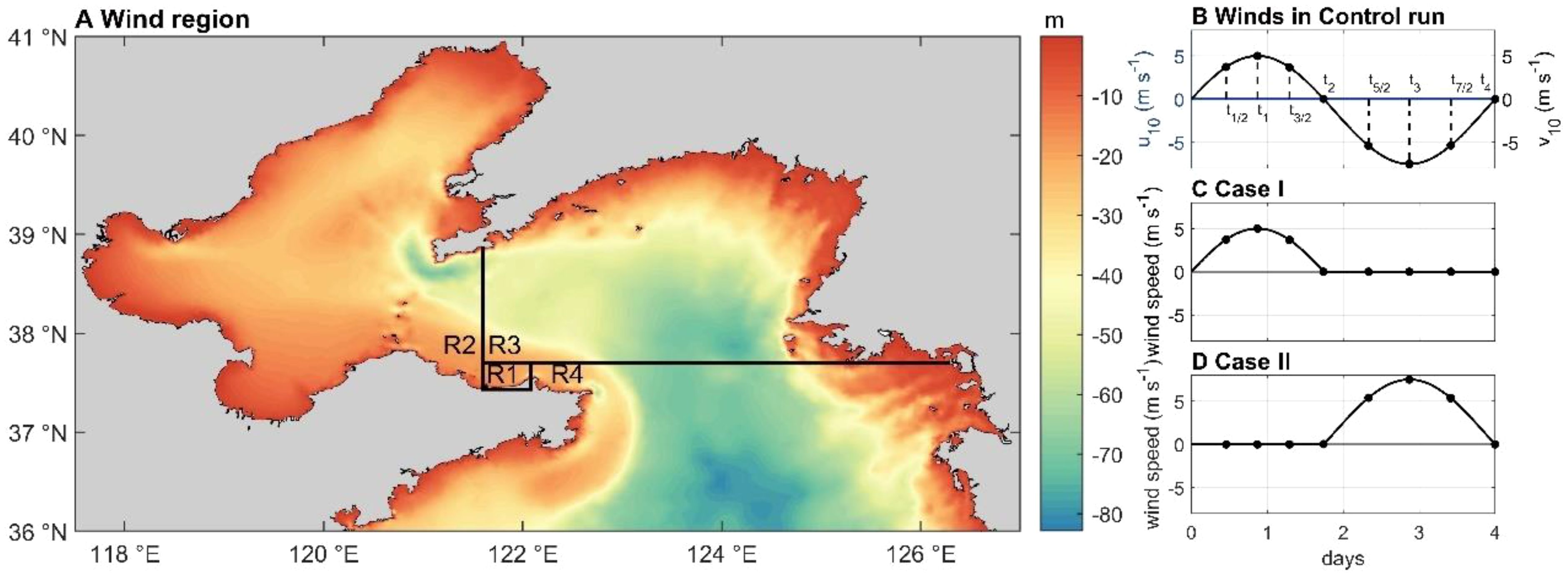
Figure 2. (A) Model domain of experiments. R1-R4 represented four regions and R1 was the study area. Sea surface winds were set to 0 except the selected region in each experiment. (B) Zonal component (blue line; m s⁻¹) and meridional component (black line; m s⁻¹) of surface winds in control run. Three time (t_1/2, t_1, t_3/2) equally divided the period of southerly winds. Three time (t_5/2, t_3, t_7/2) equally divided the period of northerly winds. (C) Surface wind speed in Case I in experiments. (D) Surface wind speed in Case II in experiments. Magnitude of wind speeds in Case I and Case II were same as contemporary meridional winds in control run.

Note that there were strong northerly winds and weak southerly winds in the Bohai Sea and North Yellow Sea in winter. Sea surface winds set up in the control run were as follows:

$\begin{array}{ll}\{\begin{array}{c}{u}_{10}=0\\ v_{10}=-1.25+6.25sin(\frac{\pi }{2d}t+{\omega }_0),0\le t<4d\\ v_{10}(t=0)=0\\ v_{10}(t=t_2 or t_4)=0\end{array}& (1)\end{array}$

where d represented one day. $u_{10}$ and $v_{10}$ were zonal and meridional components of the 10 m wind (Figure 2B). We choose three times (t_1/2, t_1, t_3/2), which equally divided the period of southerly winds. Three times (t_5/2, t_3, t_7/2) equally divided the period of northerly winds. Note that sea surface winds were spatially constant in the wind zone. Sea surface wind speeds in Case I were setup as:

$\begin{array}{ll}\{\begin{array}{c}u= -1.25+6.25sin(\frac{\pi }{2d}t+{\omega }_0), 0\le t<t_2\\ u=0,t_2\le t<4d\\ u(t=0)=0\\ u(t=t_2)=0\end{array}& (2)\end{array}$

where d represented one day and u represented sea surface wind speed (Figure 2C). Sea surface wind speed in Case II were set as:

$\begin{array}{ll}\{\begin{array}{c}u= 0, 0\le t<t_2\\ u=1.25-6.25sin(\frac{\pi }{2d}t+{\omega }_0),t_2\le t<4d\\ u(t=0)=0\\ u(t=t_2)=0\end{array}& (3)\end{array}$

where d represented one day and u represented wind speed (Figure 2D). The list of information about three series of experiments were provided in Table 1.

Table 1

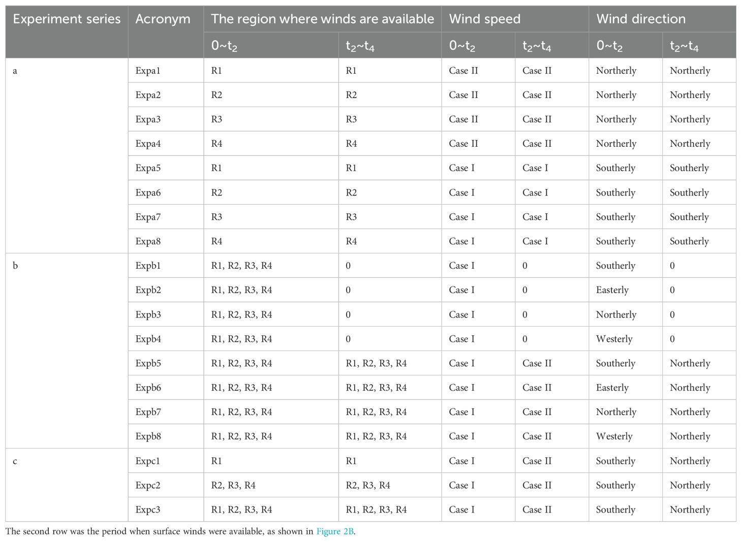
Table 1. Setup for three series of experiments.

Performance of the model simulation was validated with observations using three statistical parameters, which were simultaneous linear correlation coefficient (R), mean absolute bias (MAB), and root mean square error (RMSE). For time series or space maps of X and Y, $R=X\text{'}Y\text{'}/\sqrt{X{\text{'}}^{2}Y{\text{'}}^2}$, $MAB=\left|X-Y\right|$, and $RMSE=\sqrt{{(X-Y)}^2}$, where $X\text{'}$ and $Y\text{'}$ were anomalies, and $\langle \rangle$ denoted the time mean. Simultaneous linear correlation coefficients were all significant above the 95% confidence level unless otherwise specified.

3 Nearshore overturning currents

3.1 Model validation

Model results were evaluated with the satellite observations, atmospheric reanalysis, and SCROS observation. As shown in Figure 3, climatological winter mean SST in the model simulation showed high spatial correlations with those in the OSTIA (R=0.90), ERA5 (R=0.91) and MUSST (R=0.89). All four products clearly showed a warm tongue extending northward in the central area and cold waters in the coastal areas in the Yellow Sea in winter (Figures 3A–C). In the majority of the study area, SSTs in the model simulation showed high correlation coefficients (>0.9), low mean absolute biases (<1.0°C), and low root mean square errors (<1.0°C) with those in the other three ocean products (Figures 3D–L). Relatively large mean absolute biases and root mean square errors mainly occurred in the nearshore areas, possibly due to that both the model simulation and satellite observations contained certain errors in such shallow waters near the land. However, we noted that both mean absolute biases and root mean square errors were much smaller in the northeastern coastal waters of the Shandong Peninsula and Qinhuangdao than in other coastal waters of the Bohai Sea and Yellow Sea. This finding indicated that model-simulated SSTs agreed with satellite-observed SSTs and ERA5-reanalyzed SSTs in both magnitudes and spatiotemporal variations in the study area.

Figure 3

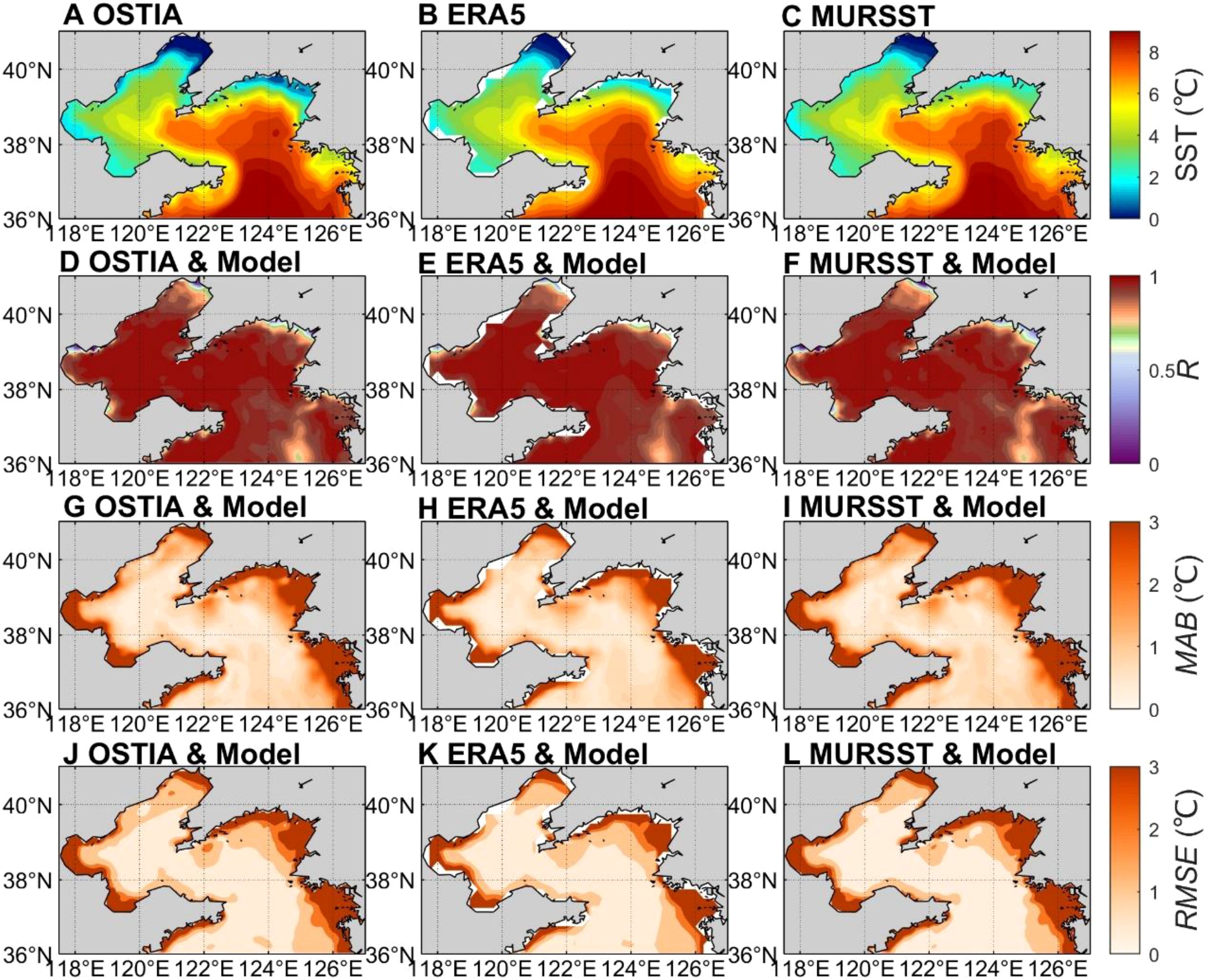
Figure 3. Comparison of daily SST (°C) in the model simulation with those in OSTIA, ERA5 and MURSST in the Bohai Sea and Yellow Sea in winters of 2019−2021. Climatological winter mean SST in (A) OSTIA, (B) ERA5 and (C) MURSST. Simultaneous linear correlation coefficients of daily SST in the model simulation with those in (D) OSTIA, (E) ERA5 and (F) MURSST. Mean absolute biases (°C) of daily SST in the model simulation with those in (G) OSTIA, (H) ERA5 and (I) MURSST. Root mean square error (°C) of daily SST in the model simulation with those in (J) OSTIA, (K) ERA5 and (L) MURSST.

During the observation period, the SCROS stayed at the sea bottom. Therefore, the observed water depth variations were equivalent to SSH variations. In the current study, we calculated SSH anomaly (SSHA) as water depth minus its time mean with the SRCOS observation and as SSH minus its time mean with the model simulation. In the study area, hourly SSHA was dominated by tidal variations (Chen et al., 2019). As shown in Figure 4, hourly (daily) SSHA in the model simulation had a R=0.77 (0.88), MAB=0.30 m (0.07 m), and RMSE=0.35 m (0.09 m) with those in the SCROS observation. This finding indicated that both hourly and daily SSHAs in the model simulation agreed with those in the SCROS observation.

Figure 4

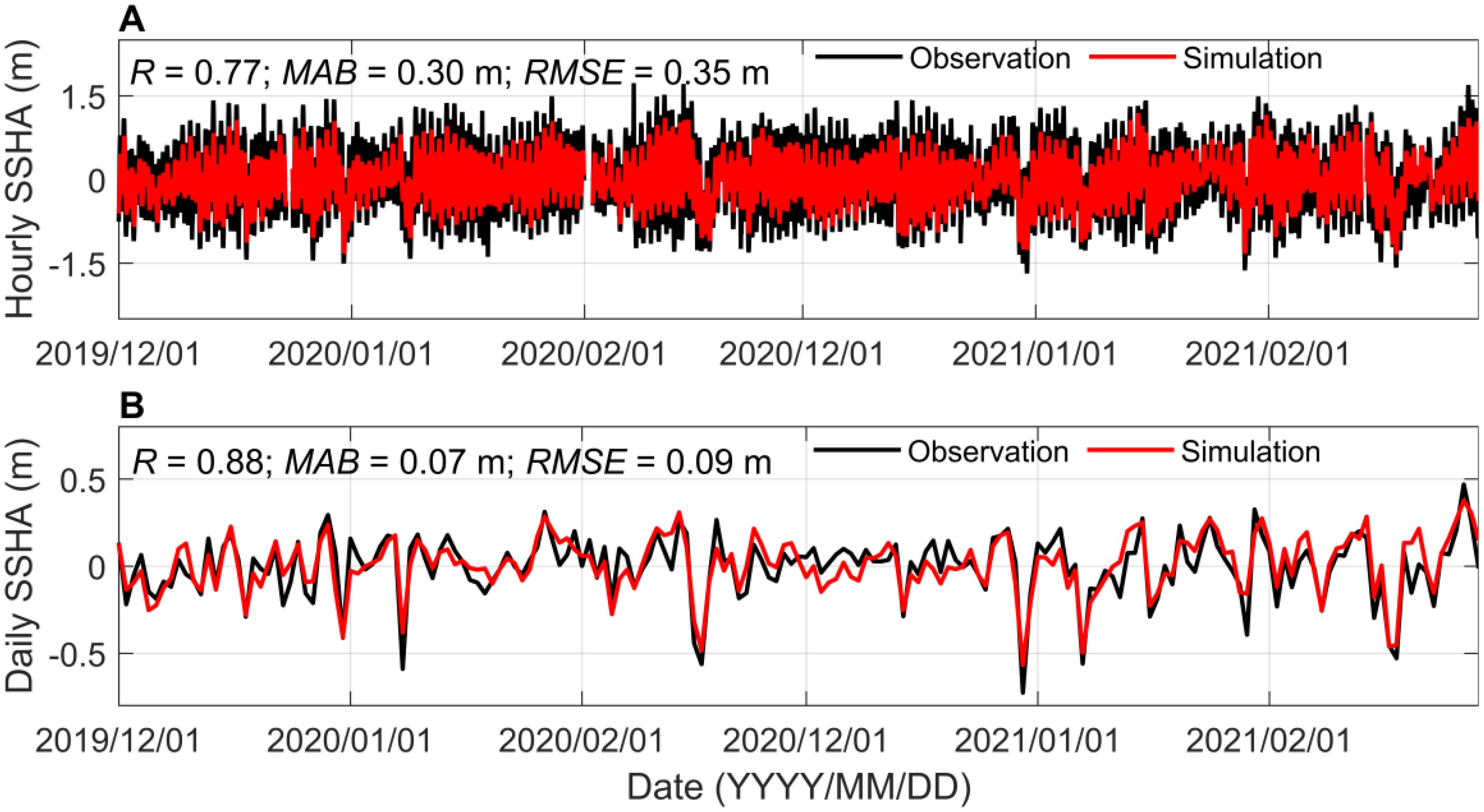
Figure 4. (A) Hourly sea surface height anomaly (SSHA; m) from SCROS observation (black line) and model simulation (red line) in the Yutai marine ranching area off the northeastern Shandong Peninsula. The three numbers indicate simultaneous linear correlation coefficient (R), mean absolute bias (MAB; m) and root mean square error (RMSE; m) between the time series. (B) Same as (A) but for daily SSHA (m).

The model-simulated tidal currents agreed with the SCROS-observed tidal currents. Figures 5A–D further compared the daily currents in the SCROS observation and model simulation. Overall, model-simulated daily currents agreed with observed daily currents in temporal variations, with simultaneous linear correlation coefficients ranging 0.56−0.74 for zonal currents and 0.50−0.76 for meridional currents. Zonal currents mostly had the same sign throughout the water column, but their speeds basically decreased from surface to bottom. On the contrary, meridional currents generally had a two-layer overturning structure, with opposite signs in the upper and lower layers (Hu et al., 2021; Zhai et al., 2021c). Model-simulated meridional currents mostly agreed with observed meridional currents in magnitude throughout the water column except in the surface layer where the model results were much smaller than the observations. The discrepancy between the simulated and observed surface meridional currents was possibly because that the model was unable to well resolve the surface current variations at the SCROS site which was so close to the shoreline (Figure 1C).

Figure 5

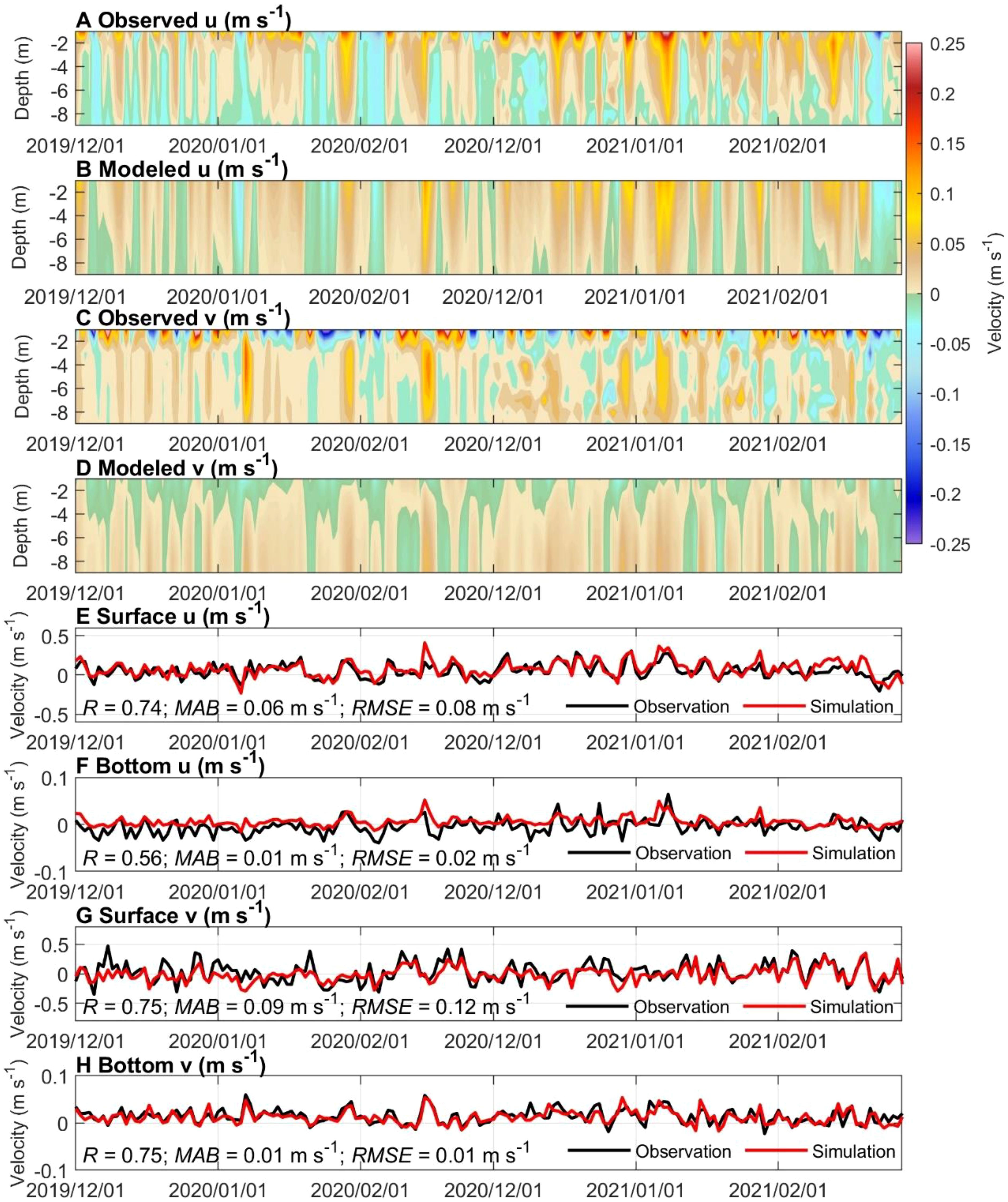
Figure 5. Comparisons of daily ocean currents (m s⁻¹) in the observation and model simulation in the Yutai marine ranching area in winters of 2019/2020 and 2020/2021. (A) Daily profiles of zonal velocity in the observation. (B) Daily profiles of zonal velocity in the model simulation. (C) Daily profiles of meridional velocity in the observation. (D) Daily profiles of meridional velocity in the model simulation. (E) Daily surface zonal velocity in the observation and model simulation. (F) Daily bottom zonal velocity in the observation and model simulation. (G) Daily surface meridional velocity in the observation and model simulation. The model-simulated meridional velocity was multiplied by 10.15 for clarity. (H) Daily bottom meridional velocity in the observation and model simulation.

Figures 5E–H presented the daily time series of surface and bottom currents in the model simulation and SCROS observation. In the surface layer, the simulated and observed zonal (meridional) currents had R=0.74 (0.75), MAB=0.06 m s⁻¹ (0.09 m s⁻¹), and RMSE=0.08 m s⁻¹ (0.12 m s⁻¹). In the bottom layer, the simulated and observed zonal (meridional) currents had R=0.56 (0.75), MAB=0.01 m s⁻¹ (0.01 m s⁻¹), and RMSE=0.02 m s⁻¹ (0.01 m s⁻¹).

Based on the above comparisons, we could conclude that the model simulation was reliable in examining the nearshore circulation dynamics off the northeastern Shandong Peninsula in the Yellow Sea in winter.

3.2 Composite analysis

As shown in Figure 5, there were strong daily variations in ocean currents in the Yutai marine ranching area off the northeastern Shandong Peninsula. In the following, days with surface meridional currents in the Yutai marine ranching area being smaller than −0.71 m s⁻¹ were defined as Period I, while those with surface meridional currents in the Yutai marine ranching area being larger than 0.56 m s⁻¹ were defined as Period II. Figure 6 presented the composite maps of SSH and current vectors during Period I and Period II to examine the three-dimensional structure of overturning currents in the study area. As shown in the figure, ocean currents basically decreased approaching the shoreline but their directions were quite different in the surface and bottom layers in both periods. In Period I, SSH basically increased approaching the shoreline and southeastward currents prevailed in the surface layer in the whole study area (Figure 6A). On the contrary, ocean currents shifted from being eastward in offshore areas to being northeastward in nearshore areas in the bottom layer. This finding indicated that the zonal components of ocean currents were mostly eastward in both the surface and bottom layers but the meridional components of ocean currents showed an overturning structure in nearshore regions. To give more details of the overturning current structure, we calculated the composited ocean currents along the meridional section at 121.92°E and showed the results in Figure 6C. As clearly seen from the figure, overturning currents in nearshore waters in Period I were composed of shoreward currents in the upper layer, downwelling near the shore, and seaward currents in the lower layer.

Figure 6

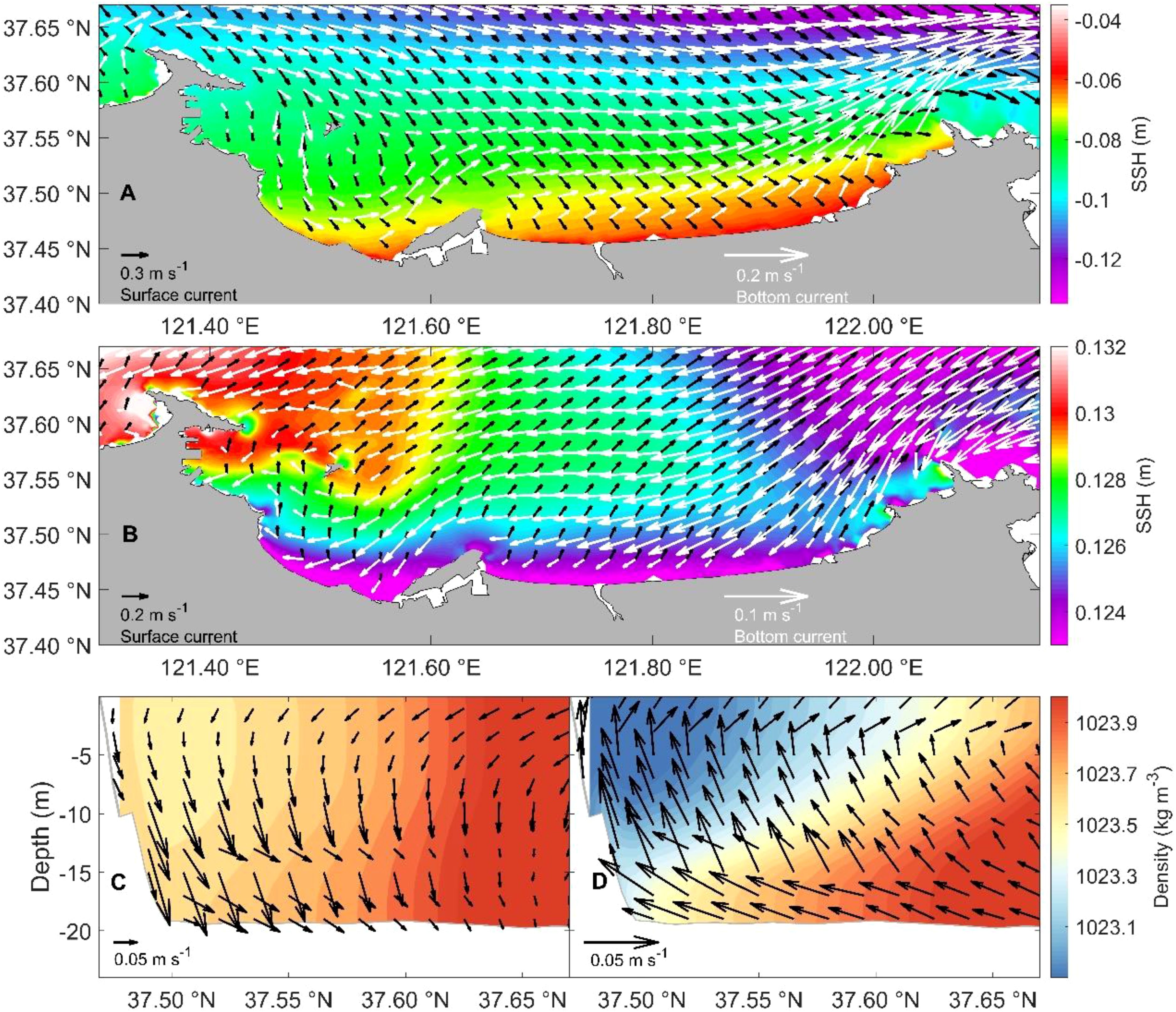
Figure 6. (A) Composite maps of current vectors (m s⁻¹) in the surface layer (black arrows) and bottom layer (white arrows) in coastal waters of the northeastern Shandong Peninsula in Period I (B) Same as (A) but in Period II. (C) Composite meridional and vertical components of ocean currents (m s⁻¹) along the meridional section at 121.92°E in coastal waters of the northeastern Shandong Peninsula in Period I (D) Same as (C) but in Period II. In (C, D), vertical components of ocean currents were multiplied by 1000 for clarity.

In Period II, however, SSH basically increased away from the shoreline and northeastward currents prevailed in the surface layer in the whole study area (Figure 6B). In the bottom layer, ocean currents shifted from being westward in offshore areas to being southwestward in nearshore areas. Clearly, bottom layer currents in Period II were nearly opposite to those in Period I. This finding indicated that ocean currents experienced more significant vertical changes in Period II than in Period I. Not only the meridional components but also the zonal components of ocean currents had opposite directions in the surface and bottom layers in Period II, which were different from the vertical structure of ocean currents in Period I. As clearly seen from Figure 6D, overturning currents in nearshore waters in Period II were composed of seaward currents in the upper layer, upwelling near the shore and shoreward currents in the lower layer.

Figure 7 presented the composite vertical profiles of ocean currents at 121.92°E, 37.65°N in the offshore area and at 121.92°E, 37.5°N in the nearshore area off the northeastern Shandong Peninsula during Period I and Period II. Overall, current speeds shared the same vertical structure in the whole study area in both periods. With increasing depth, current speeds first decreased from being largest at the sea surface to a local minimum in the middle layer, and then increased to a secondary maximum near the sea bottom. In contrast, current directions showed opposite vertical structures in the two periods. With increasing depth, current directions rotated counterclockwise in Period I but rotated clockwise in Period II. The rotation of current directions with increasing depth became more significant approaching the shoreline. The above findings indicated that ocean currents in different layers in the two periods were controlled by different mechanisms.

Figure 7

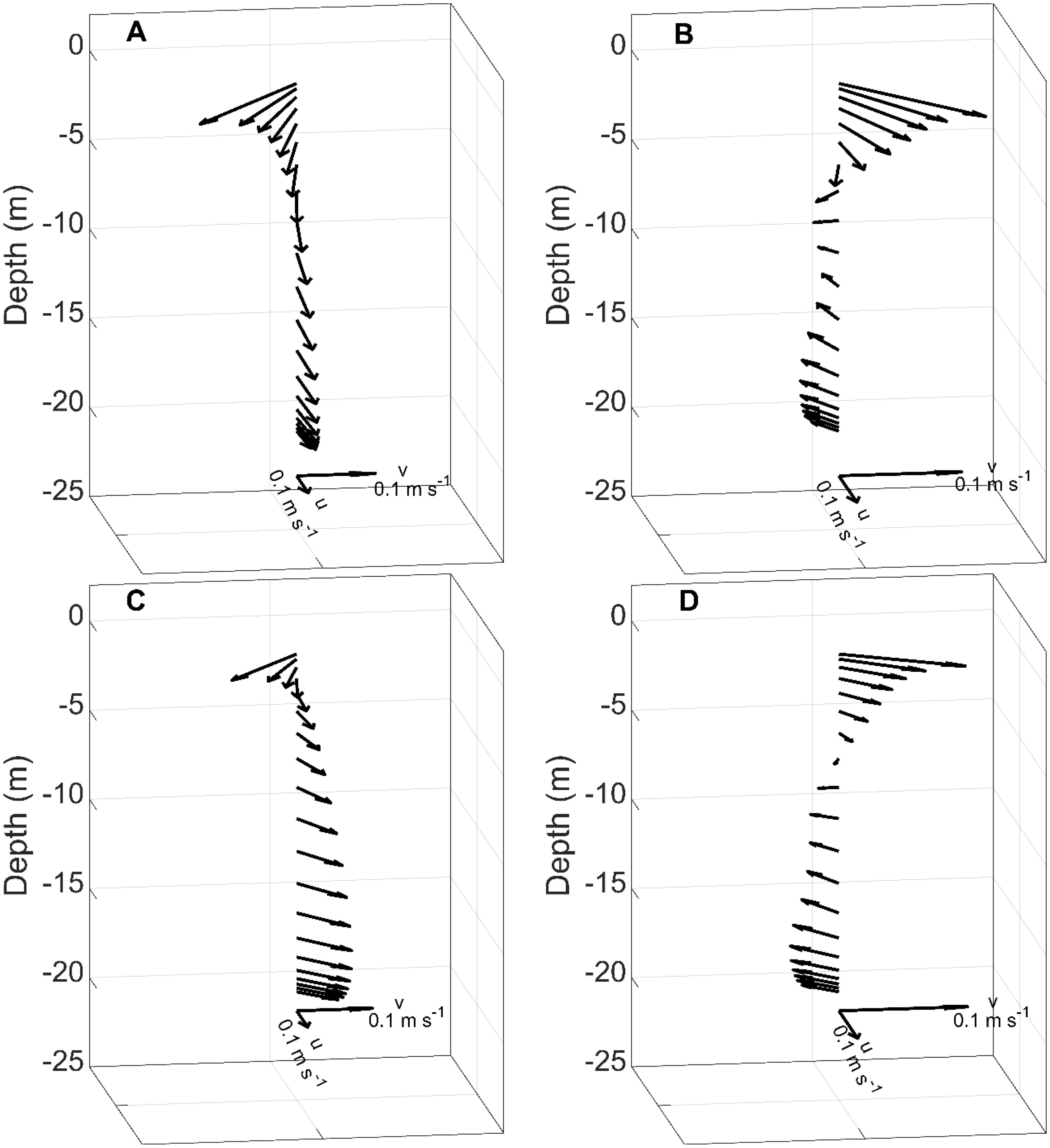
Figure 7. Composite maps of vertical profiles of horizontal currents (m s⁻¹) at (A) 121.92°E, 37.65°N in Period I, (B) 121.92°E, 37.65°N in Period II, (C) 121.92°E, 37.5°N in Period I and (D) 121.92°E, 37.5°N in Period II. The horizontal coordinate axes are rotated counterclockwise to clearly display currents.

4 Mechanisms

4.1 Wind-driven and pressure gradient-driven currents

In winter, nearshore waters of the Yellow Sea and Bohai Sea are vertically mixed throughout the water column (Zhai et al., 2021c; Liu et al., 2023). As a result, ocean currents in the nearshore waters are primarily driven by sea surface wind and pressure gradient, which results from the horizontal variations in SSH and water density. In order to check the impacts of sea surface wind and horizontal pressure gradient on ocean currents, we firstly calculated the zonal ($u_{geo}$) and meridional ($v_{geo}$) geostrophic currents at the depth of h as $u_{geo}=-\frac{g}{f}\frac{\partial \eta }{\partial y}-\frac{g}{f{\rho }_0}\underset{-h}{\overset{\eta }{\int }}\frac{\partial \rho }{\partial y}dz$ and $v_{geo}=\frac{g}{f}\frac{\partial \eta }{\partial x}+\frac{g}{f{\rho }_0}\underset{-h}{\overset{\eta }{\int }}\frac{\partial \rho }{\partial x}dz$, where positive x, y and z were eastward, northward and upward, respectively. f was the Coriolis parameter, g = 9.8 m s⁻² was gravity acceleration, η was SSH, ${\rho }_0$ = 1025 kg m⁻³ was the reference density of seawater and ρ was water density. The two terms on the right side of each equation denoted geostrophic currents caused by horizontal variations in SSH and water density, respectively. Then we calculated simultaneous linear correlation coefficients of hourly-averaged ocean currents with winds and with geostrophic currents in the zonal and meridional directions in Period I and Period II. A 25-hourly running mean filter was applied to hourly averaged data to remove tidal signals. Correlation coefficients between simulated currents and geostrophic currents caused by horizontal variations in water density were low and neglected. Figure 8 showed the simultaneous linear correlation coefficients in the surface and bottom layers. Note that geostrophic currents in Figure 8 were caused by horizontal variations in SSH. Correlations of simulated currents with geostrophic currents caused by horizontal variations in water density were weak and not shown.

Figure 8

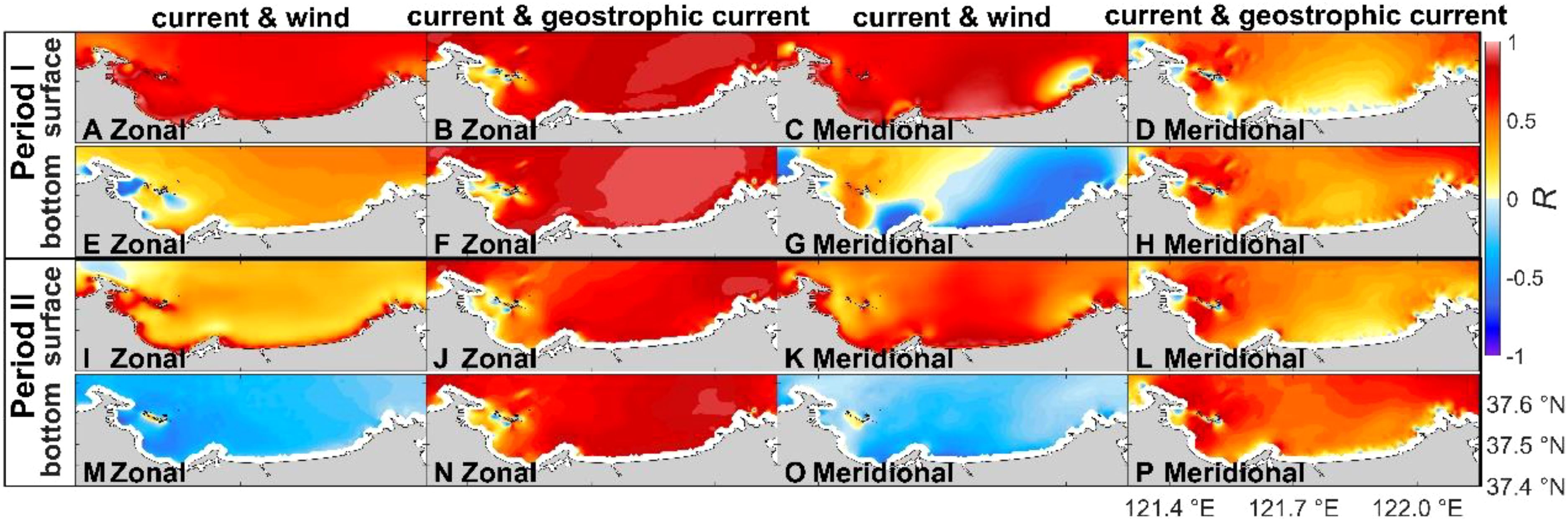
Figure 8. Simultaneous linear correlation coefficients between (A) surface zonal currents and zonal winds, (B) surface zonal currents and surface zonal geostrophic currents, (C) surface meridional currents and meridional winds, (D) surface meridional currents and surface meridional geostrophic currents. (E) bottom zonal currents and zonal winds, (F) bottom zonal currents and bottom zonal geostrophic currents, (G) bottom meridional currents and meridional winds, (H) bottom meridional currents and bottom meridional geostrophic currents in Period I (I-P) same as (A-H) but in Period II. Note that geostrophic currents here were caused by horizontal variations in SSH. Correlations of simulated currents with geostrophic currents caused by horizontal variations in water density were weak and not shown.

In Period I in the surface layer, zonal currents in the study area were strongly positively correlated with zonal geostrophic currents, with meridional currents in the surface layer positively correlated with meridional winds. In the bottom layer, zonal currents in the study area were strongly positively correlated with zonal geostrophic currents. Meridional currents in the offshore region of the study area in the bottom layer were positively correlated with meridional geostrophic currents. Meridional currents in the nearshore region of the study area in the bottom layer were negatively correlated with meridional winds. The zonal ocean currents in nearly whole study area were strongly correlated with sea level slope, while the meridional currents in the nearshore region of the study area were strongly correlated with meridional winds. This finding suggested sea level slope in the study area was not primarily caused by winds.

In Period II in the surface layer, zonal currents in the study area were strongly positively correlated with zonal geostrophic currents, with meridional currents in the surface layer positively correlated with meridional winds. In the bottom layer, zonal currents in the study area were strongly positively correlated with zonal geostrophic currents. Meridional currents in the offshore region of the study area were positively correlated with meridional geostrophic currents. Meridional currents in the nearshore region of the study area were negatively correlated with meridional winds. Distributions of simultaneous linear correlation coefficients in Period II were similar to those in Period I. However, positive correlation coefficients between zonal ocean currents and zonal geostrophic currents were significantly stronger in Period I than those in Period II. This finding suggested sea level slope might cause aforementioned distinct vertical alterations of horizontal currents in the two periods.

Based on the above results, we could conclude that zonal ocean currents in the surface and bottom layers of the study area and bottom meridional currents in the offshore region of the study area were primarily correlated with sea level slope in the two periods. Surface meridional currents in the study area and bottom meridional currents in the nearshore region of the study area were primarily correlated with meridional winds.

4.2 Momentum budgets

As shown in Figure 8, strong correlation coefficients suggested that sea level slope and winds were the robust impact factors in all two-layer ocean current events in the two periods. To gain a straight understanding of the currents driven by sea level slope and winds, it was necessary to investigate momentum budgets during a single event in Period I (Event I) and Period II (Event II). The zonal and meridional momentum balance equations with corresponding abbreviations were shown as follows:

$\begin{array}{ll}\frac{\partial u}{\underset{{\text{ACCEL}}_{\text{x}}}{\underbrace{\partial t}}}=\underset{{\text{PGF}}_{\text{x}}}{\underbrace{-\frac{1}{\rho }\frac{\partial p}{\partial x}}}\underset{{\text{ADV}}_{\text{x}}}{\underbrace{-\left(u\frac{\partial u}{\partial x}+v\frac{\partial u}{\partial y}+w\frac{\partial u}{\partial z}\right)}}\underset{{\text{COR}}_{\text{x}}}{\underbrace{+fv}}\underset{{\text{HVIS}}_{\text{x}}}{\underbrace{+\frac{\partial }{\partial x}\left(A_h\frac{\partial u}{\partial x}\right)+\frac{\partial }{\partial y}\left(A_h\frac{\partial u}{\partial y}\right)}}\underset{{\text{VVIS}}_{\text{x}}}{\underbrace{+\frac{\partial }{\partial z}\left(A_z\frac{\partial u}{\partial z}\right)}}& (4)\end{array}$

$\begin{array}{ll}\frac{\partial v}{\underset{{\text{ACCEL}}_{\text{y}}}{\underbrace{\partial t}}}=\underset{{\text{PGF}}_{\text{y}}}{\underbrace{-\frac{1}{\rho }\frac{\partial p}{\partial x}}}\underset{{\text{ADV}}_{\text{y}}}{\underbrace{-\left(u\frac{\partial v}{\partial x}+v\frac{\partial v}{\partial y}+w\frac{\partial v}{\partial z}\right)}}\underset{{\text{COR}}_{\text{y}}}{\underbrace{-fu}}\underset{{\text{HVIS}}_{\text{y}}}{\underbrace{+\frac{\partial }{\partial x}\left(A_h\frac{\partial v}{\partial x}\right)+\frac{\partial }{\partial y}\left(A_h\frac{\partial v}{\partial y}\right)}}\underset{{\text{VVIS}}_{\text{y}}}{\underbrace{+\frac{\partial }{\partial z}\left(A_z\frac{\partial v}{\partial z}\right)}}& (5)\end{array}$

where u and v were the zonal and meridional velocities and positive x, y, and z were eastward, northward, and upward, respectively. $\rho$ was the water pressure, $p$ was the water density, and $A_h$ and $A_z$ were the horizontal and vertical viscosity coefficients, respectively. The abbreviation ACCEL denoted the local acceleration term, PGF was the horizontal pressure gradient force, ADV was the three-dimensional transport term, COR was the Coriolis force, HVIS and VVIS were horizontal and vertical viscosities, respectively. ${\langle \rangle }_x$ and ${\langle \rangle }_y$ denoted the zonal and the meridional component, respectively. HVIS term was ignored because it was small. A 25-hourly running mean filter was applied to hourly averaged data to remove tidal signals. After removing tidal signals from the data, we calculated all the above terms.

Figure 9A displayed sea surface winds, surface currents, and bottom currents in the Yutai marine ranching area in Event I. On 5 January 2020, sea surface winds blew westward. Surface currents were westward and bottom currents were southward. Subsequently, both surface winds and surface currents rotated counterclockwise. On 7 January, there were strong northwesterly winds, surface southeastward currents, and bottom northeastward currents. After that, both surface winds and ocean currents weakened.

Figure 9

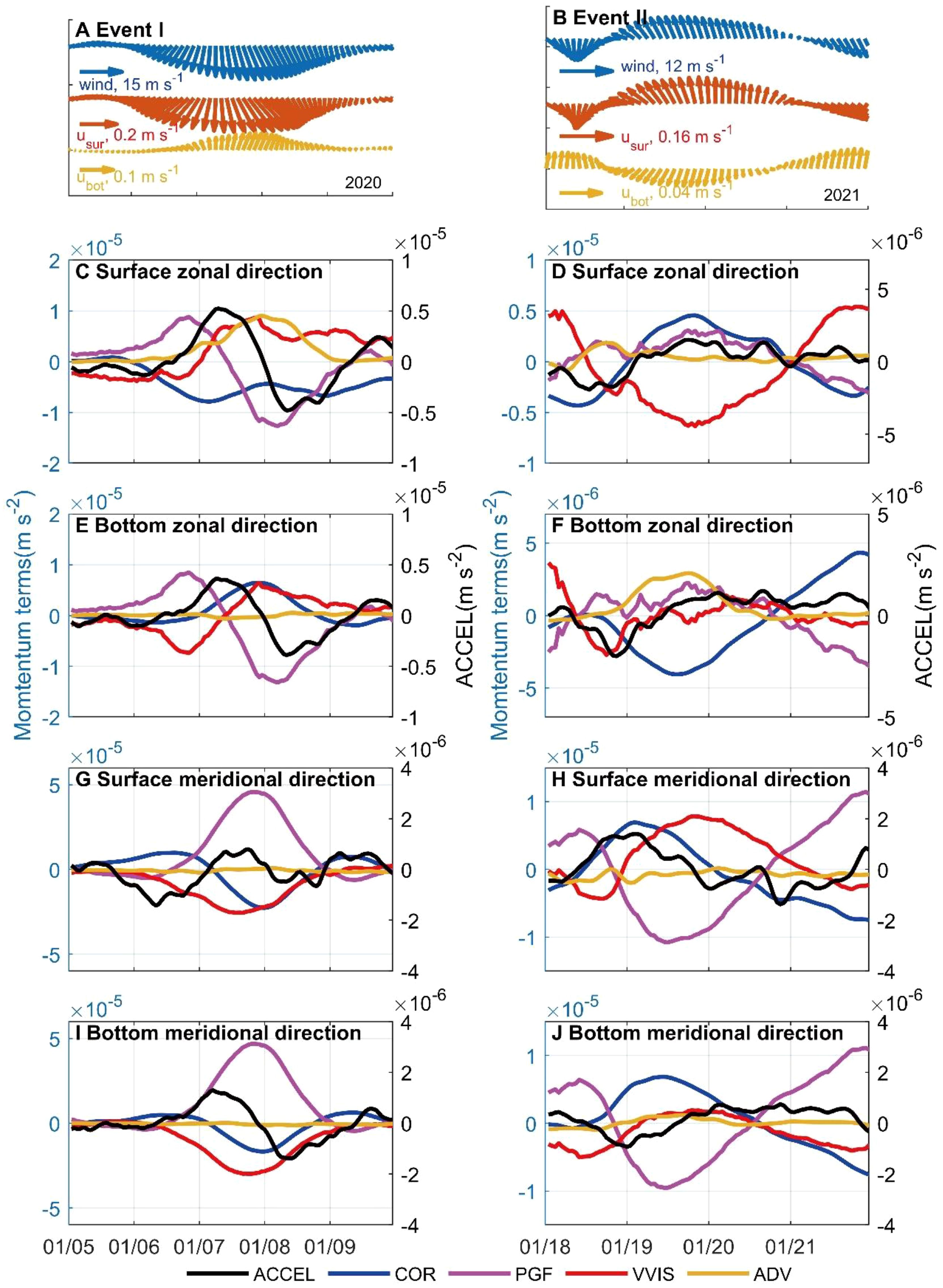
Figure 9. Sea surface winds (m s⁻¹), surface currents (m s⁻¹) and bottom currents (m s⁻¹) in the Yutai marine ranching area in (A) Event I and (B) Event II. Surface momentum terms in the Yutai marine ranching area in zonal direction in (C) Event I and (D) Event II. (E, F) Same as (C, D) but for bottom momentum terms. (G, H) Same as (C, D) but in the meridional direction. (I, J) Same as (C, D) but for bottom momentum terms.

Strong surface southward and bottom northward currents occurred on 7 January 2020 in Event I, showing two-layer ocean currents that were similar to composite results in Period I (Figure 9A). Before that on 5 January, surface westward currents were driven by easterly winds (negative surface zonal VVIS terms in Figure 9C). Then winds shifted counterclockwise and drove surface southwestward Ekman currents, which were at the right angle to the wind by surface northwestward Coriolis forces (Figure 9C; Ekman, 1905). At that time, westward sea level slope increased rapidly, which resulted in the rapid strengthening of eastward PGF (Figures 9C, E). On 7 January, the strong eastward PGF turned westward currents to the eastward in the surface and bottom layers, which were at the left angle of northerly winds (Figures 9C, E). As winds shifted southeastward, both surface eastward VVIS and PGF drove eastward currents, indicating that Ekman transport was not the main impact of westward sea level slope (Figures 9C, E). Meanwhile, southward sea level slope increased (Figure 9G). Note that northward PGF caused by southward sea level slope was stronger than surface southward VVIS caused by northerly winds and surface southward COR caused by eastward currents, so that northward PGF slowed down surface southward currents (Figure 9G). The strong northward PGF also drove bottom northward currents (Figure 9I). On 8 January 2020, sea level slope turned southeastward and slowed down eastward currents (Figures 9C, E). Meanwhile, southward sea level slope decreased rapidly so that surface southward currents increased by northerly wind and bottom northward currents weakened by bottom friction (Figures 9G, I). After that, ocean currents decreased as both wind and sea level slope decreased.

Figure 9B displayed sea surface winds, surface currents, and bottom currents in the Yutai marine ranching area in Event II. At 12:00 on 18 January 2021, there were northerly winds, surface southward currents, and bottom northward currents (Figure 9B). Then surface winds and surface currents rotated clockwise. Sea surface winds shifted to the southeasterly at 22:00 on 19 January 2021, and surface currents shifted to be northward and bottom currents shifted to be southwestward. Then, both sea surface winds and ocean currents weakened.

Strong surface northward and bottom southwestward currents occurred at 22:00 on 19 January 2021 in Event II, showing two-layer ocean currents that were similar to composite results in Period II (Figure 9B). Before that at 12:00 on 18 January, there were surface southward VVIS caused by northerly winds and northward PGF in the surface and bottom layers caused by southward sea level slope, with PGF stronger than VVIS (Figures 9H, J). From 12:00 on 18 January to 00:00 on 19 January, winds shifted clockwise to northeasterly and drove surface southeastward Ekman currents, which were at the right angle to the wind by surface northwestward Coriolis forces (Figure 9D). At that time, southward sea level slope decreased rapidly (Figures 9H, J). Bottom southward friction decreased bottom northward currents so that bottom eastward COR weakened. Bottom westward friction drove bottom westward currents with bottom eastward COR decreasing and caused bottom northward COR. Then sea level slope turned northward. Bottom southward PGF and bottom southward friction turned bottom northward currents to southward, which caused bottom westward COR. This suggested that bottom Ekman layer was regulated by bottom COR and bottom frictions when sea level slope changed (Figures 9F, J). From 00:00 on 19 January to 22:00 on 19 January 2021, surface southeasterly winds drove northwestward Ekman currents (Figure 9D). At that time, northward sea level slope increased. The strong sea level slope caused strong southward PGF, which prevented the development of surface northward currents and strengthened bottom northward currents (Figures 9H, J). After 22:00 on 19 January 2021, southeasterly winds weakened rapidly (Figures 9D, H). Strong southward PGF slowed down surface northward currents (Figure 9H). Bottom friction weakened bottom southward currents as northward sea level slope decreased (Figure 9J).

Momentum terms demonstrated that ocean currents were dominated by winds and horizontal pressure gradient in both Event I and Event II and proved that horizontal pressure gradient caused by sea level slope in the study area was not primarily caused by winds. Therefore, ocean currents and sea level were displayed to find the factors that drove sea level slope in Event I and Event II. Figures 10A–E displayed surface winds, depth-averaged currents, and sea level characteristics in Bohai Sea and North Yellow Sea in Event I. On 5 January 2020, easterly winds drove water converging in the western part of the Bohai Sea (Figure 10A). From 6 January to 8 January as winds turned counterclockwise, high sea level moved eastward along northern coastline of the Shandong Peninsula (Figures 10B–D). At this time, depth-averaged currents were southeastward, almost parallel to sea level contours. Sea level decreased with contours parallel to coastline as the offshore distance increased, exhibiting the propagation of CTWs (Wang et al., 2020; Li and Huang, 2019). After 9 January, high sea level moved to the South Yellow Sea, there were northward currents in the center of the North Yellow Sea resulting in sea level rising (Figure 10E).

Figure 10

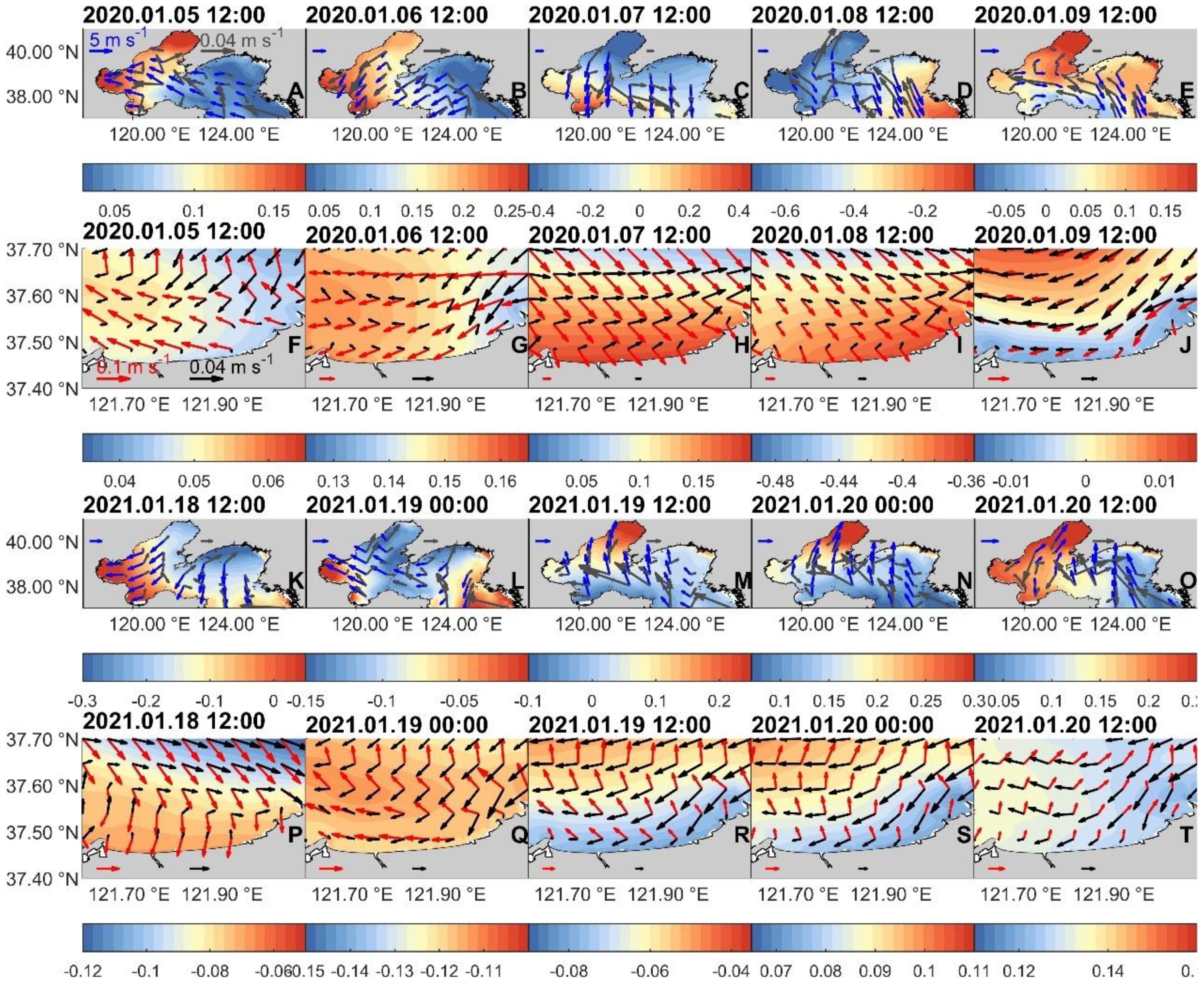
Figure 10. (A-E) Sea surface winds (blue arrows; m s⁻¹), depth-averaged currents (grey arrows; m s⁻¹) and SSH (colormap; m) in the Bohai Sea and North Yellow Sea in Event I. (F-J) Surface currents (red arrows; m s⁻¹), bottom currents (black arrows; m s⁻¹) and SSH (colormap; m) in the study area in Event I. (K-O) Same as (A-E) but in Event II. (P-T) Same as (F-J) but in Event II.

Figures 10F–J displayed surface and bottom currents and SSH in the study area (Figure 1C) in Event I. Sea surface winds in the study area were almost consistent with contemporary sea surface winds in the North Yellow Sea and not shown. On 5 January 2020, there were surface northwestward currents and bottom southwestward currents with southeasterly winds (Figure 10F). From 6 January to 7 January, CTWs of high sea level propagated to the study area and caused westward sea level slope (Figures 10G, H). Westward sea level slope caused eastward PGF and turned westward currents to eastward currents in the surface and bottom layers. The propagation of CTWs raised sea level in the nearshore region of the study area rapidly, which caused southward sea level slope and strong northward PGF (Figures 10H, I). As westward currents turned eastward, both currents and sea level were generally in agreement with composite results. After 9 January, there were westward geostrophic currents caused by northward sea level slope when sea level rose in the center of the North Yellow Sea (Figure 10J).

Figures 10K–O displayed surface winds, depth-averaged currents, and SSH in the Bohai Sea and North Yellow Sea in Event II. There were CTWs of high sea level along the northern coastline of the Shandong Peninsula and northerly winds in the North Yellow Sea at 12:00 on 18 January (Figure 10K). From 12:00 on 18 January to 00:00 on 19 January, high sea level in the south part of North Yellow Sea moved eastward when winds in the North Yellow Sea rotated clockwise (Figures 10K, L). From 19 to 20 January, southeasterly winds in the Bohai Sea and North Yellow Sea drove water diverging in the south part of the Bohai Sea and North Yellow Sea, resulting in CTWs with low sea level along the northern coastline of the Shandong Peninsula (Figures 10M, N). Then CTWs with low sea level moved eastward when winds weakened, followed by CTWs with high sea level (Figure 10O).

CTWs with high sea level caused southward sea level slope in the study area at 12:00 on 18 January (Figure 10K). Then as high sea level moved eastward, southward sea level slope decreased, resulting in the decreasing of northward PGF (Figure 10P). At 19 January, CTWs with low sea level were generated by southeasterly winds in the Bohai Sea and North Yellow Sea (Figures 10L, Q). From 19 to 20 January, CTWs passed through the study area and caused southward sea level slope in the study area, resulting in strong northward PGF (Figures 10R, S). Meanwhile, surface and bottom currents were consistent with the composite results. After low sea level moved eastward, the high sea level gradually extended to the study area (Figure 10T).

4.3 Numerical experiments

Because nearshore currents were strong daily variations and sea surface winds were complex synoptic variable in the Bohai Sea and North Yellow Sea in winter, conceptual experiments with idealized winds focused on ocean currents driven by local winds and by the propagation of CTWs were adapted to better illustrate dynamic processes of two-layer overturning currents. Figure 11 displayed results of the control run. Low (high) sea level appeared and moved eastward along coastline of northeastern Shandong Peninsula with southerly (northerly) winds developing and relaxing, which was consistent with CTWs aforementioned. Additionally, there were surface northward currents and bottom southwestward currents at t_1/2 and t₁. There were surface southeastward currents and bottom northeastward currents at t₃ and t_7/2. The general characteristics of two-layer overturning currents in the study area and CTWs in the Bohai Sea and North Yellow Sea obtained from idealized model were almost consistent with those in realistic model presented in the previous sections.

Figure 11

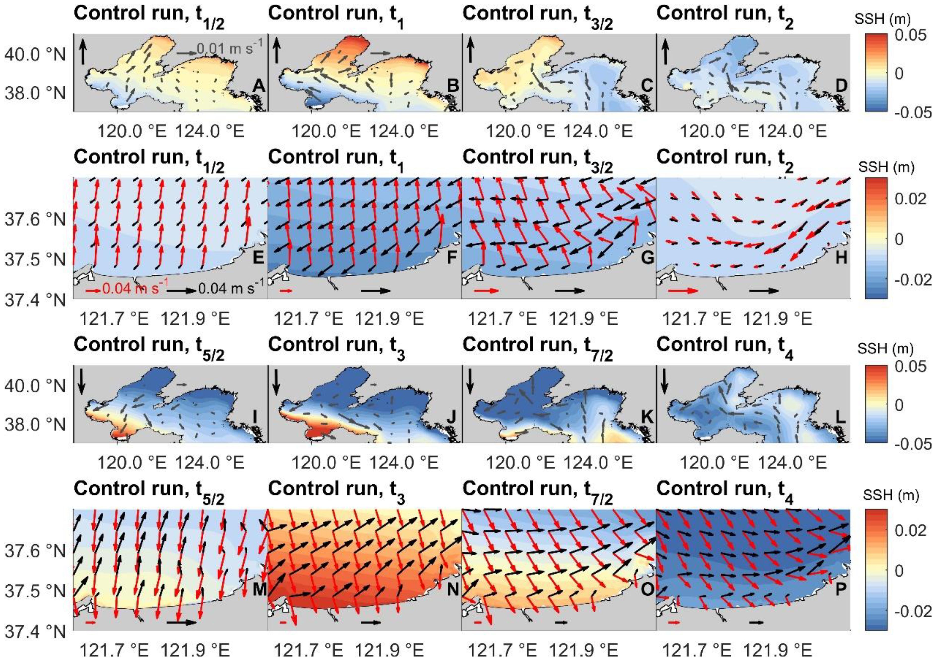
Figure 11. (A-D) Characteristics of depth-averaged currents (grey arrows; m s⁻¹) and SSH (colormap; m) in the Bohai and North Yellow Seas in the control run during southerly winds. (E-H) Characteristics of surface currents (red arrows; m s⁻¹), bottom currents (black arrows; m s−1) and SSH (colormap; m) in the study area in the control run during southerly winds. (I-L) same as (A-D) but during northerly winds. (M-P) same as (E-H) but during northerly winds. Black arrows in (A-D, I-L) were wind directions. The time of snapshot was shown in Figure 2B.

Figure 12 displayed results of the region experiments. In Expa1 (Expa5) where sea surface winds in R1 were available, sea surface winds drove surface southward (northward) currents, resulting in nearshore water convergence (divergence) and sea level rising (dropping). Then, southward (northward) sea level slope drove bottom northward (southward) currents. The northerly (southerly) winds caused sea level in the southwestern area of R1 rising (dropping). There were geostrophic currents rotating clockwise (counterclockwise) around high (low) sea level at the left boundary of R1 and counterclockwise (clockwise) around low (high) water level at the right boundary of R1. In Expa2 (Expa6), the northerly (southerly) winds caused sea level at the south boundary of R2 rising (dropping). High (low) sea level extended eastward along the coastline. Even though there was no wind in R1, the nearshore sea level rose (dropped). The southward (northward) sea level slope drove strong northeastward (southwestward) currents in the bottom Ekman layer, whose horizontal currents turned anticlockwise and weakened from surface layer to bottom layer. Both sea level slope and ocean currents were strong in the nearshore region. In Expa3 (Expa7), the northerly (southerly) winds converged (diverged) the sea level at the south boundary of R3 so that there were weak southwestward (northeastward) currents in R1. In Expa4 (Expa8), currents in the study area were much smaller than those in other experiments, indicating that winds in R4 played little impact on sea water in R1. Ocean currents in R1 were mainly driven by winds in R1 and sea level slope from R2. Additionally, as wind reversed both wind-driven currents and sea level slope driven currents reversed.

Figure 12

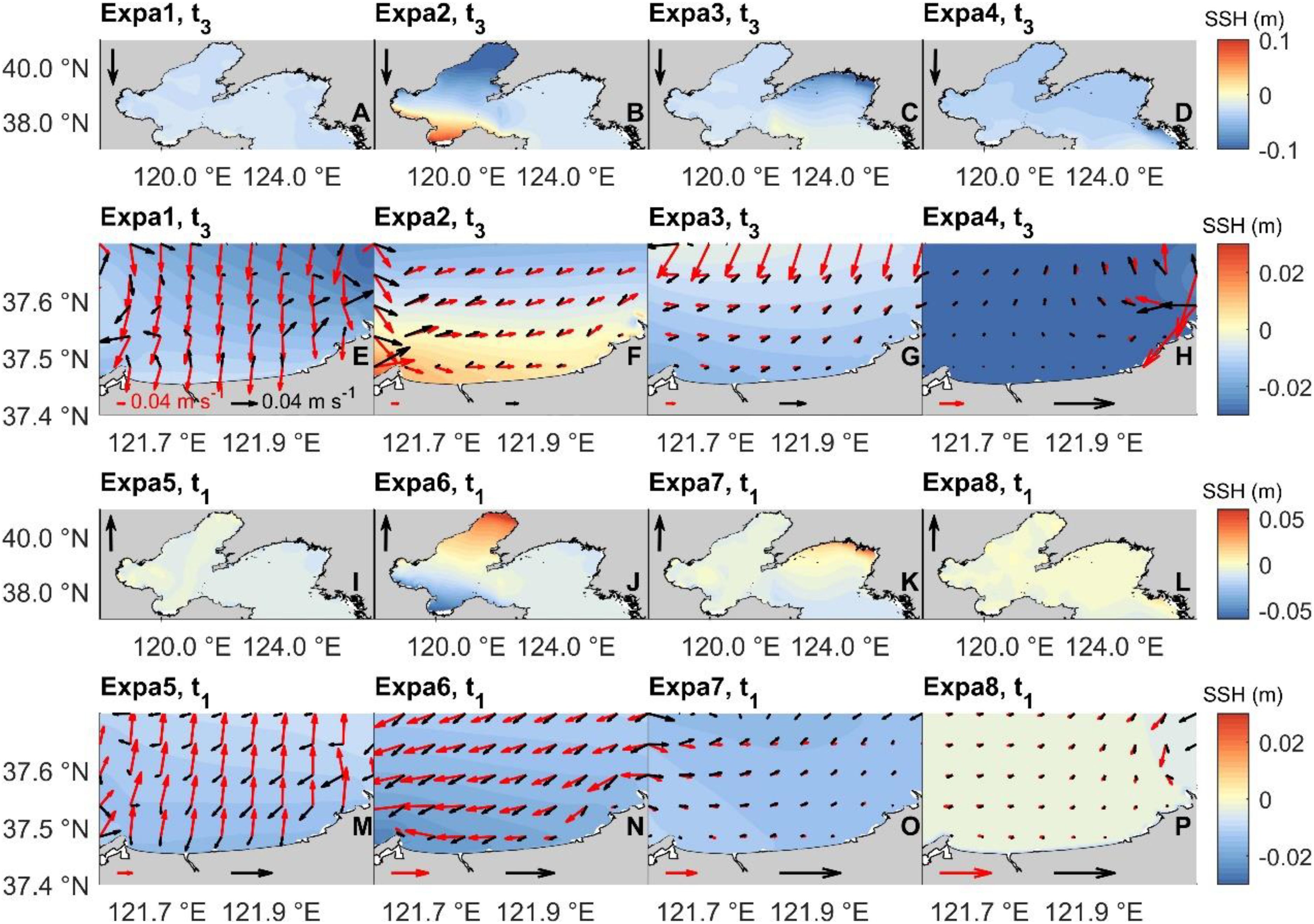
Figure 12. (A-D) SSH (m) in the Bohai Sea and North Yellow Sea and (E-H) surface currents (red arrows; m s⁻¹), bottom currents (black arrows; m s−1) and SSH (colormap; m) in R1 at t₃ when northly winds were strong in region experiments. (I-L) Same as (A-D) but at t₁ when southerly winds were strong. (M-P) Same as (E-H) but at strong southerly winds. Black arrows in (A-D) and (I-L) were wind directions. The time of snapshot was shown in Figure 2B.

Figure 13 showed sea level of CTWs in the Bohai Sea and North Yellow Sea in the experiments where wind directions were changed. Sea level rose (dropped) in the southern part of Bohai Sea and North Yellow Sea when northerly (southerly) winds developed. Then northerly (southerly) winds relaxed. low (high) sea level moved eastward along coastline. Meanwhile, high (low) sea level moved from northern part to western part of Bohai Sea. After that, high (low) sea level moved eastward following nearshore low (high) sea level. When easterly (westerly) winds developed, sea level rose (dropped) in the west area of Bohai Sea and dropped (rose) off the northeastern Shandong Peninsula. As easterly (westerly) winds relaxed, low (high) sea level moved eastward along coastline off the northeastern Shandong Peninsula followed by eastward high (low) sea level. Notably, as winds turned southerly, high sea level along the coastline of northeastern Shandong Peninsula was reconstructed. Then high sea level moved eastward as southerly winds relaxed.

Figure 13

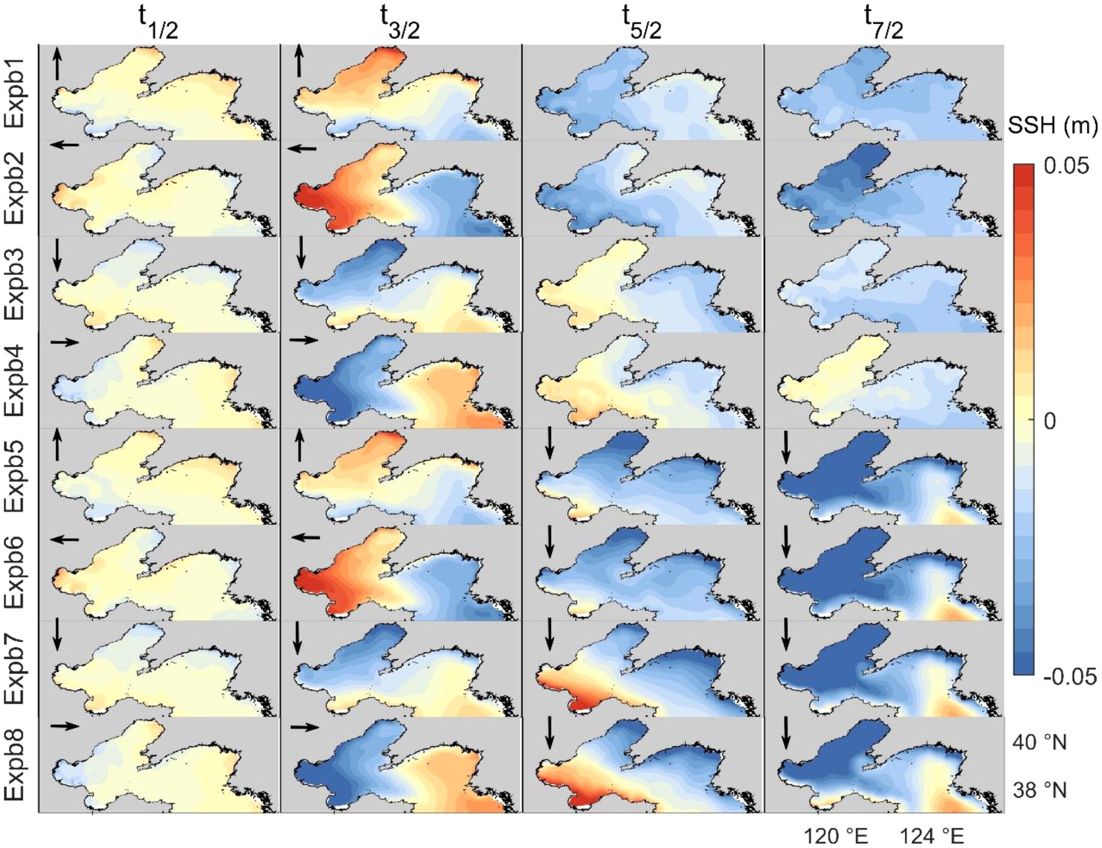
Figure 13. Sea surface height (SSH; m) in experiments where wind directions were changed. The black arrows were wind directions. The time of snapshot were shown in Figure 2B.

The evolution of wind-driven currents and geostrophic currents caused by the propagation of CTWs were explored. Model results within 121.75−121.95°E and 37.5−37.65°N were averaged and smoothed to obtain current profiles. Model results at the northern and southern boundaries of the aforementioned rectangular area were selected to calculate meridional sea level difference (MSLD). The positive MSLD meant that offshore sea level was higher than nearshore sea level.

Figures 14A–C displayed MSLD and current profiles of Expc1. At the beginning, southerly winds drove surface northeastward Ekman currents. Sea level in the northeastern (southwestern) part of the study area rose (dropped) and MSLD was increased. Meanwhile, bottom currents were southwestward caused by northeastward sea level slope. Then southerly winds weakened, resulting in the decreasing of northeastward sea level slope. The MSLD decreased and bottom southward currents weakened with wind-driven surface northeastward currents gradually extending to bottom layer. Sea level and currents under northerly winds were opposite to those under southerly winds.

Figure 14

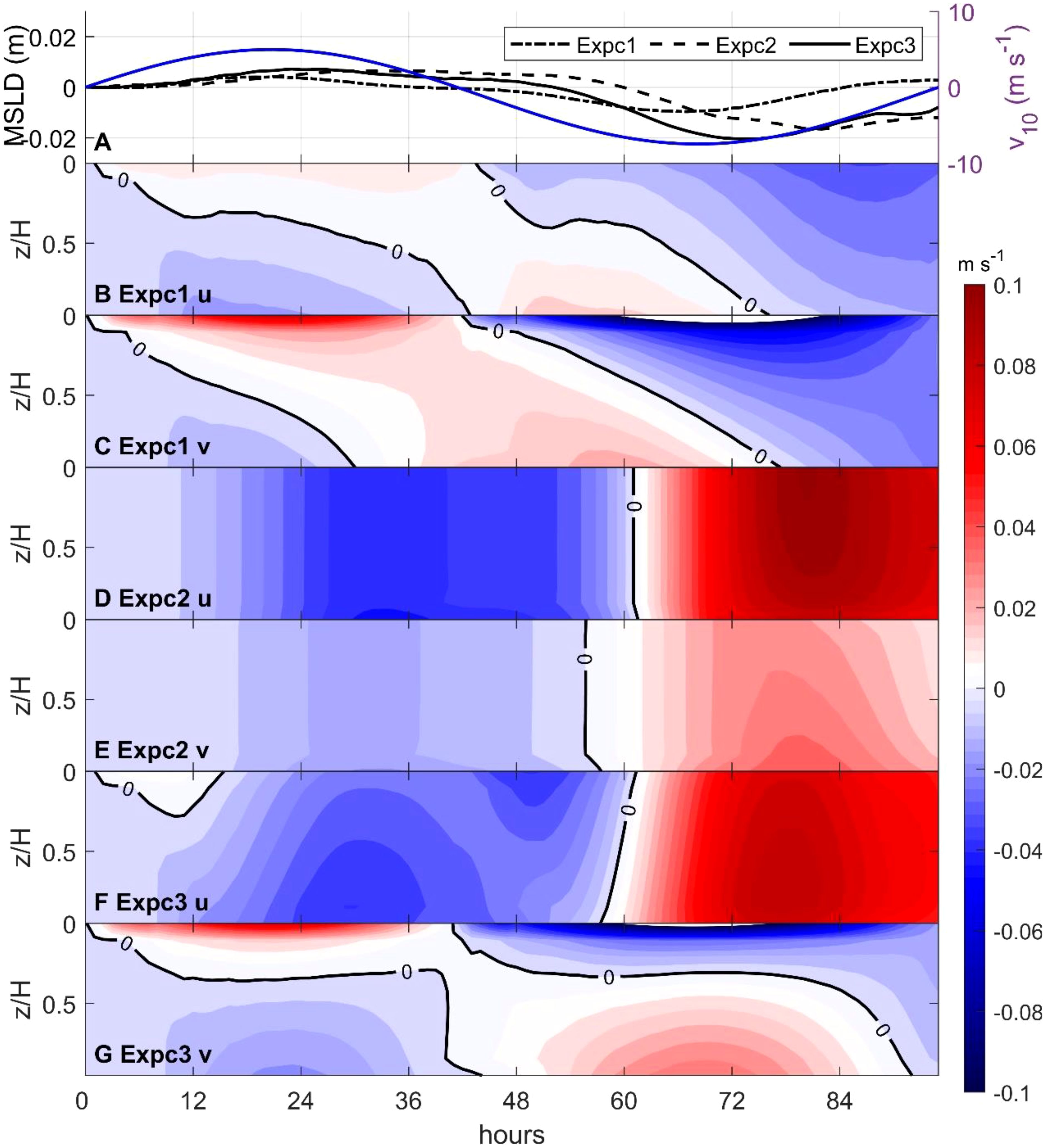
Figure 14. (A) Meridional sea level difference (MSLD; m) in the experiments. Only sea surface winds in R1 were available in Expc1. Sea surface winds in model domains were available excluding R1 in Expc2. Sea surface winds in model domain were available in Expc3. (B) Zonal and (C) meridional current profile (m s⁻¹) in Expc1. (D) Zonal and (E) meridional current profile (m s⁻¹) in Expc2. (F) Zonal and (G) meridional current profile (m s⁻¹) in Expc3.

Figures 14A, D, E displayed MSLD and current profiles of Expc2. MSLD in the study area increased when CTWs generated by southerly winds and strong westward currents occurred. Then positive MSLD and westward currents slowly decreased, even though southerly winds decreased and reserved. Subsequently, when northerly winds were strong, MSLD decreased rapidly and turned local westward currents to eastward. When the northerly winds weakened, high sea level moved eastward.

As shown in Figures 14A, F, G, MSLD and ocean currents in the study area were formed by those driven by winds in the study area and by the propagation of CTWs in the Bohai Sea and North Yellow Sea. At the beginning, southerly winds developed and diverged nearshore sea water. MSLD in Expc1 was stronger than that in Expc2 and currents in Expc3 were similar with those in Expc1, indicating that ocean currents in R1 were mainly driven by local winds. Then southerly winds were strong. MSLD in Expc2 was stronger than those in Expc1. During this period, currents driven by sea level slope of CTWs reversed surface wind-driven eastward currents but strengthened bottom southeastward currents. Horizontal currents rotated counterclockwise with increasing depth. Even though southerly winds relaxed, both MSLD and currents driven by CTWs slightly decreased. As sea surface winds reversed to northerly, southwestward currents driven by CTWs strengthened the surface wind-driven southwestward currents, weakened the bottom northward currents, and caused the bottom westward currents. Meanwhile, current directions rotated counterclockwise with increasing depth in the surface layer. Then strong northerly winds caused nearshore sea level to rise. Southward sea level slope of CTWs turned westward currents to eastward in the whole water column and strengthened bottom northward currents. At that time, current directions rotated counterclockwise with increasing depth.

5 Conclusion

The northeastern waters of the Shandong Peninsula are the nearshore area of the Bohai Sea and North Yellow Sea. There are intensive mariculture and marine ranching activities. In situ observations showed that two-layer overturning currents were robust phenomena in this area in winter. Using high-resolution numerical simulations and experiments, this current study investigated the characteristics and mechanisms of the overturning currents that have not been well established.

The results indicated that there were two classes of overturning currents (Figure 15). When there were strong southeastward currents in the surface layer, the currents in the bottom layer were northeastward. During that period, nearshore downwelling occurred. When there were strong northeastward currents in the surface layer, the currents in the bottom layer were southwestward. During that period, nearshore upwelling occurred. During both periods, the surface meridional currents were positively correlated with meridional winds. However, the ocean currents were different from wind-driven Ekman currents. The horizontal currents turned anticlockwise from surface to bottom layer when there were strong surface southeastward currents. The bottom southwestward currents were strong when there were strong surface northeastward currents.

Figure 15

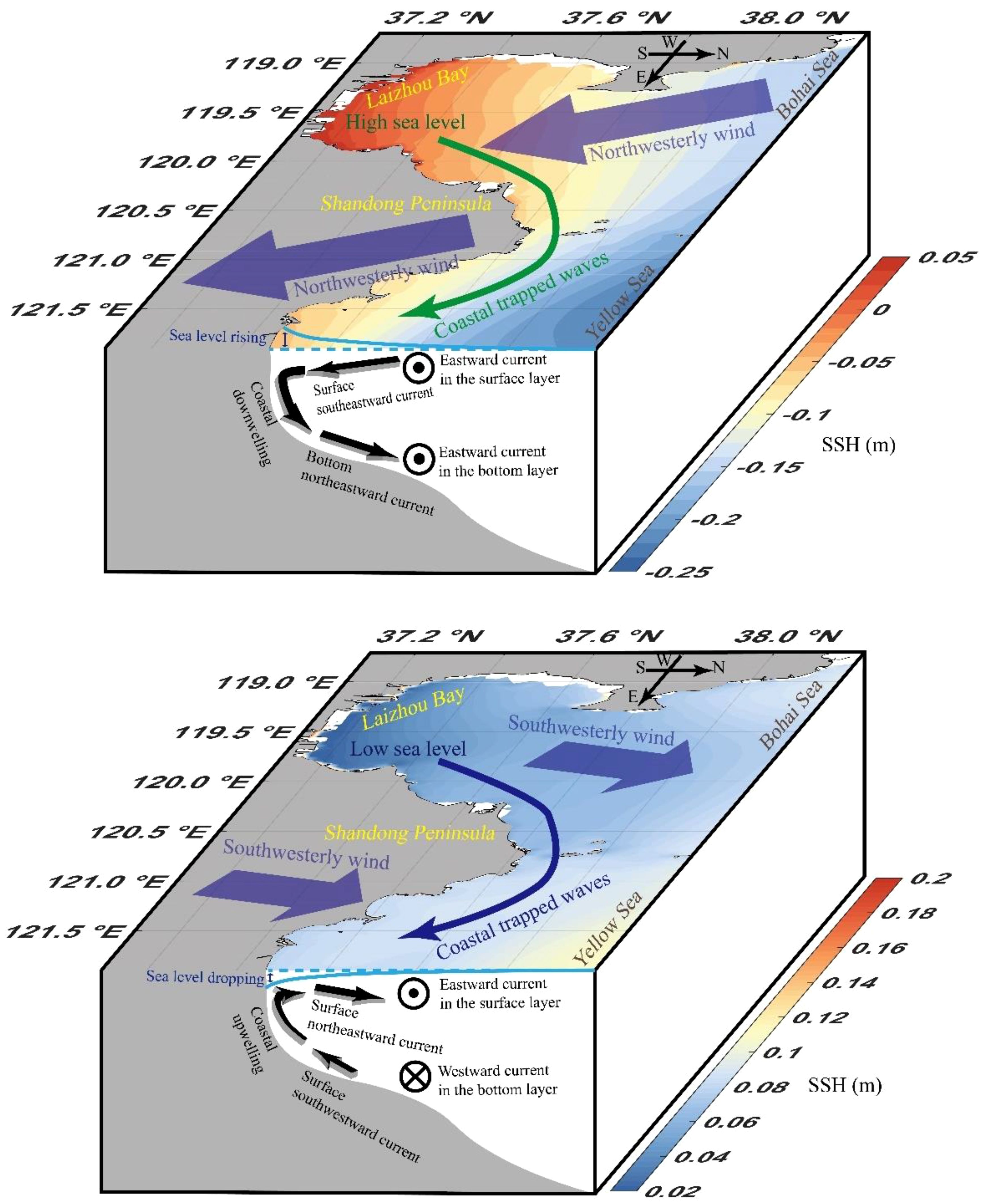
Figure 15. Schematic diagram illustrating processes responsible for two-layer overturning currents in the nearshore waters off the northeastern Shandong Peninsula in the Yellow Sea in winter.

The underlying dynamics mainly involved local wind forcing and the propagation of CTWs in the Bohai Sea and North Yellow Sea, as summarized in Figure 15. Strong surface southeastward currents occurred when there were northwesterly winds. Northwesterly winds in the study area converged water toward nearshore area so that nearshore sea level rose. Nearshore high sea level caused southward sea level slope and drove bottom northward currents. Meanwhile, northwesterly winds in the Bohai Sea and North Yellow Sea converged water toward south area of the Bohai Sea and North Yellow Sea, where sea level rose and moved eastward as CTWs. As CTWs passed through the study area, southward sea level slope of CTWs caused strong eastward in whole water column and strengthened bottom northward currents in the study area. Southwesterly winds in the study area drove surface northeastward Ekman currents and diverged nearshore water so that nearshore sea level dropped. Northward sea level slope drove bottom southward currents. Meanwhile, southwesterly winds in the Bohai Sea and North Yellow Sea diverged water in south area of the Bohai Sea and North Yellow Sea, where sea level dropped and moved eastward as CTWs. As CTWs passed through the study area, northward sea level slope of CTWs caused bottom westward currents in the study area.

The present study enriched our understanding of hydrodynamics in the nearshore marine ranching area and emphasized the importance of CTWs in the Bohai Sea and North Yellow Sea in regulating the nearshore wind-driven currents off northeastern Shandong Peninsula in winter. Note that Yellow Sea has one of the most important large marine ecosystems with intensive mariculture and marine ranching in the nearshore area. The present study showed two classes of two-layer ocean currents. This suggested the complexity variations of the surface Ekman layer and bottom Ekman layer when CTWs propagated to the study area, which could impose impacts on the nearshore marine ecosystem by Ekman transport. The variation of winds and water level in real situations are complex. Therefore, long-term observations, climatology numerical simulations, and realistic hindcast experiments according to climatology numerical simulations are needed to explore the characteristics of overturning currents. Idealized numerical experiments are needed to quantify the evolution of overturning currents under different factors.

The nearshore area connects shore and middle shelf with shallow water column. Various processes drive nearshore sea circulations, including winds, surface gravity waves, and tides (Lentz and Fewings, 2011). Although there are long-term continuous observations, high-resolution topographic data and high-quality satellite data are still needed to enrich the hydrodynamic research. Meanwhile, nearshore assimilation dataset needs to be constructed. In the future, more high-resolution observations and numerical simulations are necessary to understand the ocean currents and their impacts on biogeochemical processes in the nearshore marine ranch areas of the Yellow Sea.

Data availability statement

The original contributions presented in the study are included in the article/supplementary material. Further inquiries can be directed to the corresponding author.

Author contributions

LH: Writing – original draft, Writing – review & editing, Conceptualization, Formal analysis, Investigation, Methodology, Software, Visualization. FZ: Writing – review & editing, Conceptualization, Formal analysis, Funding acquisition, Investigation, Supervision. ZL: Data curation, Methodology, Validation, Writing – review & editing. YG: Data curation, Resources, Writing – review & editing. WW: Methodology, Software, Writing – review & editing. PL: Data curation, Resources, Writing – review & editing. JL: Data curation, Writing – review & editing. JD: Data curation, Writing – review & editing. LS: Data curation, Writing – review & editing.

Funding

The author(s) declare financial support was received for the research, authorship, and/or publication of this article. This research was funded by the National Science Foundation of China (42176016); Scientific and Technological Projects of Zhoushan (2022C01004).

Acknowledgments

Many thanks to Joseph Zhang for patiently answering all queries relating to SCHISM.

Conflict of interest

The authors declare that the research was conducted in the absence of any commercial or financial relationships that could be construed as a potential conflict of interest.

Publisher’s note

All claims expressed in this article are solely those of the authors and do not necessarily represent those of their affiliated organizations, or those of the publisher, the editors and the reviewers. Any product that may be evaluated in this article, or claim that may be made by its manufacturer, is not guaranteed or endorsed by the publisher.

References

Austin J. A., Lentz S. J. (2002). The inner shelf response to wind-driven upwelling and downwelling. J. Phys. Oceanography 32, 2171–2193. doi: 10.1175/1520-0485(2002)032<2171:TISRTW>2.0.CO;2

Crossref Full Text | Google Scholar

Chen Y., Gao L., Liu Z., Sun L., Gu Y., Zhai F., et al. (2019). Tidal characteristics of marine pastures around Shandong Peninsula. Oceanologia Et Limnologia Sin. 50, 719−727. doi: 10.11693/hyhz20180900227

Crossref Full Text | Google Scholar

Chin T. M., Vazquez-Cuervo J., Armstrong E. M. (2017). A multi-scale high-resolution analysis of global sea surface temperature. Remote Sens. Environ. 200, 154–169. doi: 10.1016/j.rse.2017.07.029

Crossref Full Text | Google Scholar

Csanady G. T. (1973). Wind-induced barotropic motions in long lakes. J. Phys. Oceanography 3, 429–438. doi: 10.1175/1520-0485(1973)003<0429:WIBMIL>2.0.CO;2

Crossref Full Text | Google Scholar

Donlon C. J., Martin M., Stark J. D., Roberts-Jones J., Fiedler E., Wimmer W. (2012). The operational sea surface temperature and sea ice analysis (OSTIA) system. Remote Sens. Environ. 116, 140–158. doi: 10.1016/j.rse.2010.10.017

Crossref Full Text | Google Scholar

Ekman V. W. (1905). On the influence of the Earth’s rotation on ocean currents. Arkiv för matematik, astronomi och fysik, 2, 1–53. Available at: http://jhir.library.jhu.edu/handle/1774.2/33989.

Google Scholar

Garland E. D., Zimmer C. A., Lentz S. J. (2002). Larval distributions in inner-shelf waters: the roles of wind-driven cross-shelf currents and diel vertical migrations. Limnology Oceanography 47, 803–817. doi: 10.4319/lo.2002.47.3.0803

Crossref Full Text | Google Scholar

Grantham B. A., Chan F., Nielsen K. J., Fox D. S., Barth J. A., Huyer A., et al. (2004). Upwelling-driven nearshore hypoxia signals ecosystem and oceanographic changes in the northeast Pacific. Nature 429, 749–754. doi: 10.1038/nature02605

PubMed Abstract | Crossref Full Text | Google Scholar

Hersbach H., Bell B., Berrisford P., Hirahara S., Horányi A., Muñoz-Sabater J., et al. (2020). The ERA5 global reanalysis. Q. J. R. Meteorological Soc. 146, 1999–2049. doi: 10.1002/qj.3803

Crossref Full Text | Google Scholar

Hsueh Y. (1988). Recent current observations in the eastern Yellow Sea. J. Geophysical Res. 93, 6875–6884. doi: 10.1029/JC093iC06p06875

Crossref Full Text | Google Scholar

Hsueh Y., Pang I. C. (1989). Coastally trapped long waves in the Yellow Sea. J. Phys. Oceanography 19, 612–625. doi: 10.1175/1520-0485(1989)0192.0.CO;2

Crossref Full Text | Google Scholar

Hu L., Zhai F., Liu Z., Li P., Gu Y., Sun L., et al. (2021). Spatial and temporal characteristics of sea current within the marine ranches in the northeast of Shandong Peninsula. Mar. Sci. 45, 1−12. doi: 10.11759/hykx20200811003

Crossref Full Text | Google Scholar

Kämpf J. (2017). Wind-driven overturning, mixing and upwelling in shallow water: A nonhydrostatic modeling study. J. Mar. Sci. Eng. 5, 47. doi: 10.3390/jmse5040047

Crossref Full Text | Google Scholar

Lentz J., Fewings R. (2011). The Wind- and Wave-driven inner-shelf circulation. Annu. Rev. Mar. Sci. 4, 317–343. doi: 10.1146/annurev-marine-120709-142745

Crossref Full Text | Google Scholar

Li Z., Huang D. (2019). Sea surface height and current responses to synoptic winter wind in the Bohai, Yellow, and East China Seas: Two leading coastal trapped waves. J. Geophysical Research: Oceans 124, 2289–2312. doi: 10.1029/2018jc014120

Crossref Full Text | Google Scholar

Li H., Zhai F., Dong Y., Liu Z., Gu Y., Bai P. (2024). Interannual-decadal variations in the Yellow Sea Cold Water Mass in summer during 1958–2016 using an eddy-resolving hindcast simulation based on OFES2. Continental Shelf Res. 275, 105223. doi: 10.1016/j.csr.2024.105223

Crossref Full Text | Google Scholar

Lin X. P., Yang J. Y. (2011). An asymmetric upwind flow, Yellow Sea Warm Current: 2. Arrested topographic waves in response to the northwesterly wind. J. Geophysical Res. 116, C04027. doi: 10.1029/2010JC006514

Crossref Full Text | Google Scholar

Lin X. P., Yang J. Y., Guo J. S., Zhang Z. X., Yin Y. Q., Song X. Z., et al. (2011). An asymmetric upwind flow, Yellow Sea Warm Current: 1. New observations in the western Yellow Sea. J. Geophysical Res. 116, C04026. doi: 10.1029/2010JC006513

Crossref Full Text | Google Scholar

Liu Z., Zhai F., Gu Y. (2023). Observed current variations in the Bohai Sea in the winter of 2020/2021. J. Sea Res. 196, 102450. doi: 10.1016/j.seares.2023.102450

Crossref Full Text | Google Scholar

Lyard F., Allain D., Cancet M., Carrère L., Picot N. (2021). FES2014 global ocean tide atlas: design and performance. Ocean Sci. 17, 615−649. doi: 10.5194/os-17-615-2021

Crossref Full Text | Google Scholar

Qu L., Lin X., Hetland R. D., Guo J. (2018). The asymmetric continental shelf wave in response to the synoptic wind burst in a semienclosed double-shelf basin. J. Geophysical Research: Oceans 123, 131–148. doi: 10.1002/2017JC013025

Crossref Full Text | Google Scholar

Qu T., Mitsudera H., Yamagata T. (1999). A climatology of the circulation and water mass distribution near the philippine coast. J. Phys. Oceanography 29, 1488−1505. doi: 10.1175/1520-0485(1999)029<1488:ACOTCA>2.0.CO;2

Crossref Full Text | Google Scholar

Roberts K., Pringle W., Westerink J. (2019). OceanMesh2D 1.0: MATLAB-based software for two-dimensional unstructured mesh generation in coastal ocean modeling. Geoscientific Model. Dev. 12, 1847–1868. doi: 10.5194/gmd-12-1847-2019

Crossref Full Text | Google Scholar

Su J. L. (2001). A review of circulation dynamics of the coastal oceans near China. Acta Oceanologica Sin. 23, 1–16. doi: 10.3321/j.issn:0253-4193.2001.04.001

Crossref Full Text | Google Scholar

Su J. L., Yuan Y. L. (2005). China Offshore Hydrology (Beijing: China Ocean Press).

Google Scholar

Takahashi S., Isoda Y., Yanagi T. (1995). A numerical study on the formation and variation of a clockwise-circulation during winter in the Yellow Sea. J. Oceanography 51, 83–98. doi: 10.1007/BF02235938

Crossref Full Text | Google Scholar

Tilburg C. E. (2003). Across-shelf transport on a continental shelf: do across-shelf winds matter. J. Phys. Oceanography 33, 2675–2688. doi: 10.1175/1520-0485(2003)033<2675:ATOACS>2.0.CO;2

Crossref Full Text | Google Scholar

Wang C., Liu Z., Harris C. K., Wu X., Wang H., Bian C., et al. (2020). The impact of winter storms on sediment transport through a narrow strait, Bohai, China. J. Geophysical Research: Oceans 125, e2020JC016069. doi: 10.1029/2020jc016069

Crossref Full Text | Google Scholar

Wang B., Wang X., Zhan R. (2003). Nutrient conditions in the yellow sea and the east China sea. Estuarine Coast. Shelf Sci. 58, 127–136. doi: 10.1016/S0272-7714(03)00067-2

Crossref Full Text | Google Scholar

Wang J., Yu Z., Wei Q., Yao Q. (2019). Long-term nutrient variations in the Bohai Sea over the past 40 years. J. Geophysical Research: Oceans 124, 703–722. doi: 10.1029/2018JC014765

Crossref Full Text | Google Scholar

Wu W., Li P., Zhai F., Gu Y., Liu Z. (2020). Evaluation of different wind resources in simulating wave height for the Bohai, Yellow, and East China Seas (BYES) with SWAN model. Continental Shelf Res. 207, 104217. doi: 10.1016/j.csr.2020.104217

Crossref Full Text | Google Scholar

Wu W., Zhai F., Gu Y., Liu C., Li P. (2023b). Weak local upwelling may elevate the risks of harmful algal blooms and hypoxia in shallow waters during the warm season. Environ. Res. Lett. 18, 114031. doi: 10.1088/1748-9326/ad0256

Crossref Full Text | Google Scholar

Wu W., Zhai F., Liu C., Gu Y., Li P. (2023c). Three-dimensional structure of summer circulation in the Bohai Sea and its intraseasonal variability. Ocean Dynamics 73, 679–698. doi: 10.1007/s10236-023-01576-6

Crossref Full Text | Google Scholar

Wu W., Zhai F., Liu Z., Liu C., Gu Y., Li P. (2023a). The spatial and seasonal variability of nutrient status in the seaward rivers of China shaped by the human activities. Ecol. Indic. 157, 111223. doi: 10.1016/j.ecolind.2023.111223

Crossref Full Text | Google Scholar

Zhai F., Gu Y., Li P., Sun L., Li X., Chen D., et al. (2020a). Construction and development of marine ranch observation network in Shandong Province. Mar. Sci. 44, 93−106. doi: 10.11759/hykx20200623002

Crossref Full Text | Google Scholar

Zhai F., Hu D. (2013). Revisit the interannual variability of the North Equatorial Current transport with ECMWF ORA-S3. J. Geophysical Research: Oceans 118, 1349−1366. doi: 10.1002/jgrc.20093

Crossref Full Text | Google Scholar

Zhai F., Li P., Gu Y., Li X., Chen D., Li L., et al. (2020b). Review of the research and application of the submarine cable online observation system. Mar. Sci. 44, 14–28. doi: 10.11759/hykx20200331003

Crossref Full Text | Google Scholar

Zhai F., Liu Z., Li P., Gu Y., Hu L., Sun L., et al. (2021c). Monthly and interannual variations in winter positive surface-bottom temperature difference in northeastern coastal waters of the Shandong Peninsula in the Yellow Sea. J. Geophysical Research: Oceans 126, e2021JC017562. doi: 10.1029/2021JC017562

Crossref Full Text | Google Scholar

Zhai F., Liu Z., Li P., Gu Y., Sun L., Hu L., et al. (2021b). Physical controls of summer variations in bottom layer oxygen concentrations in the coastal hypoxic region off the northeastern Shandong Peninsula in the Yellow Sea. J. Geophysical Research: Oceans 126, e2021JC017299. doi: 10.1029/2021JC017299

Crossref Full Text | Google Scholar

Zhai F., Wang Q., Wang F., Hu D. (2014). Variation of the north equatorial current, mindanao current, and kuroshio current in a high-resolution data assimilation during 2008–2012. Adv. Atmospheric Sci. 31, 1445−1459. doi: 10.1007/s00376-014-3241-1

Crossref Full Text | Google Scholar

Zhai F., Wu W., Gu Y., Li P., Song X., Liu P., et al. (2021a). Interannual-decadal variation in satellite-derived surface chlorophyll-a concentration in the Bohai Sea over the past 16 years. J. Mar. Syst. 215, 103496. doi: 10.1016/j.jmarsys.2020.103496

Crossref Full Text | Google Scholar

Zhang Y., Ateljevich E., Yu H., Wu C., Yu J. (2015). A new vertical coordinate system for a 3D unstructured-grid model. Ocean Model. 85, 16−31. doi: 10.1016/j.ocemod.2014.10.003

Crossref Full Text | Google Scholar

Zhang Z., Qu F., Wang S. (2019). Sustainable development of the Yellow Sea large marine ecosystem. Deep-Sea Res. Part II 163, 102–107. doi: 10.1016/j.dsr2.2018.08.009

Crossref Full Text | Google Scholar

Zhang S., Wang Q., Lv Y., Cui H., Yuan Y. (2008). Observation of the seasonal evolution of the Yellow Sea Cold Water Mass in 1996−1998. Continental Shelf Res. 28, 442–457. doi: 10.1016/j.csr.2007.10.002

Crossref Full Text | Google Scholar

Zhang Y., Ye F., Stanev E., Grashorn S. (2016). Seamless cross-scale modeling with SCHISM. Ocean Model. 102, 64–81. doi: 10.1016/j.ocemod.2016.05.002

Crossref Full Text | Google Scholar

Zheng X. Y., Zhang H., Li Y. F., Zou T., Liu X., Xing Q. G. (2021). The features and mechanisms of the North Shandong Coastal Current: a case study in 2014. J. Oceanography 77, 631–646. doi: 10.1007/s10872-021-00597-3

Crossref Full Text | Google Scholar