A ConvLSTM nearshore water level prediction model with integrated attention mechanism

Nearshore water-level prediction has a substantial impact on the daily lives of coastal residents, fishing operations, and disaster prevention and mitigation. Compared to the limitations and high costs of traditional empirical forecasts and numerical models for nearshore water-level prediction, data-driven artificial intelligence methods can more efficiently predict water levels. Attention mechanisms have recently shown great potential in natural language processing and video prediction. Convolutional long short-term memory(ConvLSTM) combines the advantages of convolutional neural networks (CNN) and long short-term Memory (LSTM), enabling more effective data feature extraction. Therefore, this study proposes a ConvLSTM nearshore water level prediction model that incorporates an attention mechanism. The ConvLSTM model extracts multiscale information from historical water levels, and the attention mechanism enhances the importance of key features, thereby improving the prediction accuracy and timeliness. The model structure was determined through experiments and relevant previous studies using five years of water level data from the Zhuhai Tide Station and the surrounding wind speed and rainfall data for training and evaluation. The results indicate that this model outperforms the four other baseline models of PCCs, RMSE, and MAE, effectively predicting future water levels at nearshore stations up to 48 h in advance. Compared to the ConvLSTM model, the model with the attention mechanism showed an average improvement of approximately 10% on the test set, with a greater error reduction in short-term forecasts than that in long-term forecasts. During Typhoon Higos, the model reduced the MAE of the best-performing baseline model by approximately 3.2 and 2.4 cm for the 6- and 24-hour forecasts, respectively, decreasing forecast errors by approximately 18% and 11%, effectively enhancing the ability of the model to forecast storm surges. This method provides a new approach for forecasting nearshore tides and storm surges.

1 Introduction

With the intensification of climate change and frequent occurrence of marine disasters, the demand for forecasting various types of marine hazards has recently increased. Natural disasters, such as storm surges, pose considerable threats to human life and property, particularly in coastal areas. Therefore, this study aimed to explore improved methods for marine water-level prediction to enhance its accuracy and practicality.

Traditional empirical forecasts and numerical simulations have met prediction requirements to a certain extent; however, they still have limitations. Empirical forecasts often rely on personal experience and localized data, making it difficult to comprehensively consider the complexity of the marine environment. Although numerical simulation methods can accurately model changes in certain marine elements, they still face challenges in predicting highly nonlinear marine disasters, such as storm surges and hazardous waves. In addition, high computational costs and complex model structures limit the practical application of numerical simulations (Mel et al., 2014).

With the rapid development of artificial intelligence (AI) technology, deep learning models are gradually being applied to the prediction of marine elements. Early related studies Sztobryn (2003) used artificial neural networks (ANN) to predict sea-level heights and compared them with observed sea-level values, finding that neural network methods can be integrated into routine operational forecasting services alongside other conventional methods. A convolutional neural network (CNN) was utilized to forecast wind speeds 4 h in advance (Zhao et al., 2020), effectively capturing the nonlinear patterns of wind speeds; the results demonstrated the feasibility of CNN in wind speed prediction. In the field of marine forecasting, predicting water levels involves forecasting time-series data. Recurrent neural networks (RNN), which are capable of effectively predicting time series data, were previously used (Kagemoto, 2020) to forecast ocean waves and validate the effectiveness of RNNs in time series forecasting. Despite the presence of some nonlinearity in the data, good forecasting results were still achieved. Furthermore, with rapid developments in the field of AI, RNNs have evolved into several variants, such as gate recurrent units (GRU) and long short-term memory (LSTM), all of which are better suited for handling time-series data. LSTM was applied to forecast water levels at 17 stations in Taiwan, and LSTM outperformed six other models in forecasting accuracy (Yang et al., 2020).

To enhance the performance of various deep learning models, researchers often combine multiple models or structures to achieve ideal models by integrating the advantages of each structure. For instance, the accuracy of storm surge predictions was improved by combining LSTM and CNN model structures and studying a CNN-LSTM hybrid model that showed less error in short-term forecasts compared with those of individual CNN or LSTM models (Wang et al., 2021). Wave elements were predicted in the South and East China Seas using the ConvLSTM model for two-dimensional wave forecasting (Zhou et al., 2021) and demonstrated high prediction accuracy and efficiency. To predict tide levels at multiple tide stations, GRU was combined with graph neural networks (GNN) to create a graph convolutional recurrent neural network (Zhang et al., 2023), and this model forecasted future tide levels at multiple stations with higher accuracy than those of five other commonly used baseline models. A more efficient wave forecasting model, the Double-stage ConvLSTM (D-ConvLSTM), was proposed (Ouyang et al., 2023). This model outperformed ConvLSTM in terms of short-term forecasting capabilities compared to those of the ECMWF-WAM model, while saving computational resources and time.

With the outstanding performance of transformer models based on self-attention mechanisms across various fields of artificial intelligence, increased attention has been recently focused on the application of attention mechanisms (Vaswani et al., 2017). In AI, attention mechanisms are a technology that allows models to focus on important parts of information processing, akin to how humans concentrate on critical information when reading or observing (Itti et al., 1998; Corbetta and Shulman, 2002; Larochelle and Hinton, 2010). The introduction of attention mechanisms typically improves the model performance to some extent. A squeeze-and-excitation networks(SENet) module was developed (Hu et al., 2018), and it achieved good results across various classification networks at that time. The convolutional block attention module (CBAM), which does not consume excessive computational resources, enhances the target classification and detection performance in various models (Woo et al., 2018). Owing to its ability to focus on more feature information while conserving computational resources, this study integrates the CBAM module for research purposes. In tasks involving time-series prediction, CBAM enhances the model forecasting performance by capturing the attention weights of input features across channels and spatial points, enabling better identification of anomalous events in input features. The CNN and LSTM models exhibit certain limitations when predicting marine elements. For example, CNN models capture local features within datasets (LeCun et al., 1998), whereas LSTM models are suitable for capturing temporal dependencies within a time series (Hochreiter and Schmidhuber, 1997). However, when these two models are individually applied, they often fail to fully consider the comprehensive impact of the input feature time and spatial characteristics. The ConvLSTM model integrates the strengths of CNN and LSTM, demonstrating advantages in time-series prediction tasks and better handling of these tasks. Therefore, this study proposes a novel model that integrates attention mechanisms with the ConvLSTM to better predict changes in coastal water levels.

This study proposes a CBAM-ConvLSTM model for predicting water levels, which integrates the advantages of attention mechanisms, CNN, and LSTM to enhance prediction accuracy. A case study was conducted using actual measurement data from Zhuhai Station, China, and it was compared with four other models: ANN, CNN, LSTM, and ConvLSTM. Experiments were conducted to forecast the measured water levels 6, 12, 24, and 48 h in advance, employing multiple evaluation metrics to assess the models. This study provides new insights and methods for improving marine water level prediction models, thereby contributing to better safeguarding of human lives and property in coastal areas.

The remainder of this paper is organized as follows: Section 2 discusses the data and methodology used in this study; Section 3 outlines the forecasting process and model structure; Section 4 compares the tidal and storm surge forecasting results of our model with those of other baseline models; and Section 5 summarizes the conclusions and limitations of this study.

2 Data and methods

2.1 Data

The water level data used in this study were collected from hourly measurements at the Zhuhai tide station from 2016 to 2020. These data reflect the variations in water levels under different environmental conditions and provide essential foundational data for establishing prediction models. Meteorological data were sourced from the European Center for Medium-Range Weather Forecasts (ECMWF) global atmospheric reanalysis product ERA5. The selected ERA5 data included hourly records from 2016 to 2020 for the 10m u-component of wind, 10m v-component of wind, and total precipitation at a spatial resolution of 0.25° (Hersbach et al., 2023). This study exclusively employed the aforementioned data as inputs for the models because these elements constitute considerable factors contributing to nonlinear changes in water levels. Moreover, when forecasting water levels, introducing excessive inputs can lead to redundant data and hinder the ability of the model to accurately capture patterns. Therefore, this study avoided including redundant factors as much as possible. Figure 1 shows the location of Zhuhai Station.

Figure 1

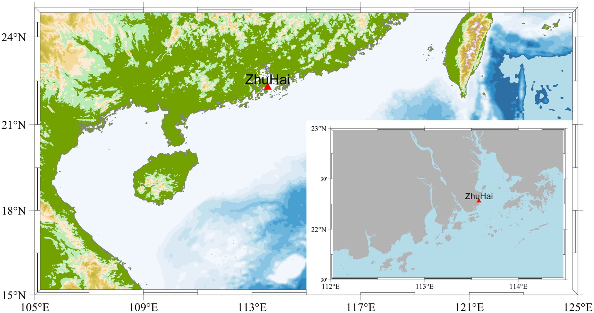
Figure 1. Zhuhai station.

2.2 Methods

2.2.1 Research problem

This study forecasted the water levels at the Zhuhai Station in advance using neural network models based on historical water level data from nearshore tidal gauge stations and weather information. Models for advanced water level prediction were trained according to the forecasting requirements. To construct the water level prediction models, this study employed various neural network models, including ANN, LSTM, CNN, ConvLSTM, and ConvLSTM with fused attention mechanisms, these models were chosen for this study because ANN, LSTM, and CNN are the classic deep learning model architectures, which are widely used in various research fields and are the more common baseline models used for comparison. ConvLSTM is able to combine the advantages of these classic models, so these neural network models are finally chosen for this study, to conduct multi-step-ahead forecasts of water levels at Zhuhai Station and the corresponding analytical research.

2.2.2 CBAM and ConvLSTM

The Convolutional Block Attention Module (CBAM) consists of two attention modules: the Channel Attention Module and the Spatial Attention Module, as illustrated in Figure 2.

Figure 2

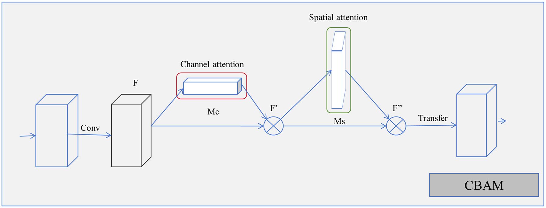
Figure 2. CBAM structure.

Channel attention in CBAM utilizes global average pooling to obtain global statistical information for each channel and employs two fully connected layers to learn the channel weights. During the propagation of the input features, the values in the channel attention structure initially undergo global average pooling. Subsequently, the pooled values are passed through a sigmoid function to normalize the weights, which are then multiplied by the corresponding channel values to acquire the global statistical information for each channel. The spatial attention module in CBAM uses max-pooling and average-pooling to extract detailed features from each spatial position. Specifically, post-convolution, which generates multiple channels, and spatial attention in CBAM apply max-pooling and average-pooling operations to each channel at every feature point. After obtaining the two matrices, they are concatenated and processed through a convolutional layer and a sigmoid function to learn the weights for each spatial position. Finally, these weights are applied to each spatial position on the feature map to produce features with enhanced spatial importance. The utilization of these attention mechanisms can effectively improve the performance of neural network models. This process is represented by the following formula:

$\begin{array}{ll}{F}^{\prime }=M_c(F)\otimes F& (1)\end{array}$

$\begin{array}{ll}\begin{array}{c}{M}_c(F)=\sigma (MLP(AvgPool(F))+MLP(MaxPool(F)))\\ =\sigma (W_1(W_0(F_{avg}^c))+W_1(W_0(F_{max}^c)))\end{array}& (2)\end{array}$

$\begin{array}{ll}{F}^{″}=M_s(F^{\prime })\otimes F^{\prime }& (3)\end{array}$

$\begin{array}{ll}\begin{array}{l}{M}_s(F)=\sigma (f^{7\times 7}([AvgPool(F);MaxPool(F)]))\\ =\sigma (f^{7\times 7}([F_{avg}^s;F_{max}^s]))\end{array}& (4)\end{array}$

where F represents the input feature values; F' denotes the feature values after passing through the channel attention module Mc(F); F'' denotes the feature values after passing through the spatial attention module Ms(F), ⊗ represents element-by-element multiplication; W0 and W1 are the weights of the MLP, σ denotes the sigmoid function, 7×7 is the convolution operation using the 7×7 convolution kernel, AvgPool and MaxPool denote global average pooling and global max pooling. During the multiplication process, attention values are broadcasted accordingly: channel attention values are broadcasted along the spatial dimensions, and F'' is the final output.

ConvLSTM is a specialized type of recurrent neural network that combines the characteristics of CNN and LSTM (Shi et al., 2015). Initially, RNNs were used to handle time-series problems; however, they encountered issues of vanishing and exploding gradients when dealing with long sequential data (Bengio et al., 1994). LSTM, which adds gate mechanisms to RNNs, partially alleviates these problems, and is more suitable for processing long sequential tasks. ConvLSTM units, building upon traditional LSTM units, replace point-wise multiplication in gate mechanisms with convolutions, enabling the simultaneous consideration of both the temporal and spatial features of the data. In ConvLSTM, convolution operations are used not only for mapping inputs to hidden states but also for computing gate signals between hidden states and mapping hidden states to outputs. This design enables ConvLSTM to capture local dependencies in spatiotemporal sequence data while retaining its ability to handle long-term dependencies, such as LSTM. With the introduction of convolution operations, ConvLSTM has become more efficient in processing high-dimensional data, achieves weight sharing, reduces the number of model parameters, and allows ConvLSTM units to process different regions of data in parallel, thereby further enhancing the computational efficiency. The ConvLSTM model itself combines the advantages of these classical ANN, CNN and LSTM models, and its forecasting performance is relatively high. Therefore, combining the attention mechanism with the ConvLSTM model can get better forecasting results than combining other baseline models.

ConvLSTM is widely used in various spatiotemporal prediction tasks, such as weather forecasting, video prediction, and traffic flow prediction. Typically, ConvLSTM uses two-dimensional image data as input, but it has been shown that using one-dimensional data can yield better prediction results than those of LSTM (Jalalifar et al., 2024). Moreover, LSTM may exhibit degraded performance when dealing with long input sequences constructed using sliding windows. In contrast, ConvLSTM can handle one-dimensional time-series data by dividing long sequences into subsequences for training. For instance, given the input of hourly water-level data of LSTM over five days, it learns the overall patterns for these five days. However, in the ConvLSTM, the data can be restructured into segmented data for each of the five days. This approach allows the model to not only learn the overall patterns but also capture finer temporal patterns within each day, thereby achieving better prediction performance. By learning the patterns of data variation over time, the ConvLSTM can extract features at various timescales, thus generating relatively accurate predictions of future states.

$\begin{array}{ll}it=\sigma (W_{xi}*X_t+W_{hi}*H_{t-1}+W_{ci}\circ C_{t-1}+b_i)& (5)\end{array}$

$\begin{array}{ll}ft=\sigma (W_{xf}*X_t+W_{hf}*H_{t-1}+W_{cf}\circ C_{t-1}+b_f)& (6)\end{array}$

$\begin{array}{ll}Ct=ft\circ C_{t-1}+it\circ tanh(W_{xc}*X_t+W_{hc}*H_{t-1}+b_c)& (7)\end{array}$

$\begin{array}{ll}ot=\sigma (W_{xo}*X_t+W_{ho}*H_{t-1}+W_{co}\circ C_t+b_o)& (8)\end{array}$

$\begin{array}{ll}{H}_t=ot\circ tanh(C_t)& (9)\end{array}$

where it represents the input gate, Ct is the memory gate, ft is the forget gate, ot is the output gate, Ht is the final unit output, and $\circ$ is hadamard product. ConvLSTM shares a similar overall structure with LSTM, featuring 3-gate structures. The difference is that the convolution kernel in each gate * represents convolution.

In this study, the features outputted by the ConvLSTM units were fed into the CBAM module to extract the attention weights between each unit, followed by spatial attention weight calculations on the input feature maps to obtain attention-enhanced feature maps. By introducing the attention module, the ConvLSTM model focuses more on learning the salient parts of the data, thereby improving the prediction of actual changes in water levels. In water level data, variations often resemble tidal changes; however, during typhoon impacts, the changes in water level are substantially larger than usual. Owing to the scarcity of data influenced by typhoons, conventional neural network models tend to have larger forecasting errors for this subset of water-level data. ConvLSTM has the advantage of handling time-series data. The CBAM module provides more parameters that can help the model notice potential changes in water level characteristics, and the CBAM module can notice the importance of the data between channels and input sequences, compared with the general channel attention module can learn more details to improve the performance of the model. This study introduces the CBAM module on top of the ConvLSTM to enhance the ability of the model not only to accurately forecast tides but also to pay more attention to the law of storm surges and the details of water level change and obtain a neural network model with a better forecast effect.

2.2.3 Evaluation metrics

During testing, the following metrics were used to evaluate the performances of the neural networks: Mean Absolute Error (MAE), Pearson product-moment correlation coefficient (PCCs), and root-mean-squared error (RMSE). These evaluation indicators are commonly used indicators for deep learning applications in the marine field, which can visualize the advantages and disadvantages of the model results for subsequent analysis and research. The formulas are expressed as follows:

$\begin{array}{ll}MAE=\frac{1}{n}{\displaystyle {\sum }_{i=1}^n|X_i-Y_i|}& (10)\end{array}$

$\begin{array}{ll}PCCs=\frac{{\displaystyle {\sum }_{i=1}^n(X_i-\overline{X})(Y_i-\overline{Y})}}{\sqrt{{\displaystyle {\sum }_{i=1}^n{(X_i-\overline{X})}^2}}\sqrt{{\displaystyle {\sum }_{i=1}^n{(Y_i-\overline{Y})}^2}}}& (11)\end{array}$

$\begin{array}{ll}RMSE=\sqrt{\frac{1}{n}{\displaystyle {\sum }_{i=1}^n}{{(X_i-Y_i)}^2}^{}}& (12)\end{array}$

where n is the number of data points, $X_i$ is the predicted value at the i-th data point; and $Y_i$ is the true value at the i-th data point. Smaller MAE and RMSE values indicate smaller errors between the predicted and actual values, whereas larger PCCs indicate a higher similarity between the predicted and actual curves. This study used these evaluation metrics to assess the results of predicting water levels at 6, 12, 24, and 48 h ahead for each model.

3 Prediction models

3.1 Model forecasting process

In this study, the CBAM module was integrated into the ConvLSTM model to obtain a fused attention mechanism for water-level prediction. The input-output relationships and feature propagation of the model are shown in Figure 3.

Figure 3

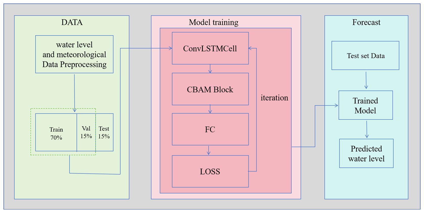
Figure 3. Model prediction process.

The training process can be divided into three major modules: data preprocessing, model training, and model prediction. First, the model was subjected to data preprocessing. Hourly time-series data for wind speed and precipitation in terms of longitude and latitude were averaged from nine grid points near the research station. Values obtained through linear regression were used to fill missing or abnormal values. The input data were screened to ensure quality and reliability. Interpolation was performed to maintain data integrity and continuity. Subsequently, the data were normalized to ensure that each feature had a similar scale and distribution. Normalization prevents input features of different magnitudes from affecting the model training weights, thereby enhancing the robustness and stability of the model. The normalization formula is as follows:

$\begin{array}{ll}{Y}_i=\frac{X_i-X_{min}}{X_{max}-X_{min}}& (13)\end{array}$

where Y_i represents the normalized data; X_i represents the data before preprocessing, X_max and X_min represent the minimum and maximum values of the data for each feature, respectively.

After data preprocessing, the processed data were divided into a 70% training set, 15% validation set, and 15% test set. The training and validation data were inputted into the model for iterative training. During training, the ConvLSTM units in the model learned the temporal features of the data, followed by training with the CBAM module to help the model focus on important features within the input data. Subsequently, the final output was obtained through the fully connected layers and compared with the label data to compute the loss. After multiple training iterations, a well-trained water-level forecasting model was obtained. The test set was then fed into the trained water level forecasting model to obtain the predicted water levels. Finally, the predicted water levels were evaluated against the test labels using metrics, such as MAE, RMSE, and PCCs for model assessment.

3.2 Model construction

To analyze and compare the forecasting results, this study employed baseline models, such as ANN, CNN, LSTM, and ConvLSTM, in addition to the CBAM-ConvLSTM model. ANN is a computational model that simulates a network of neurons in the human brain, processing information through weighted sums and nonlinear activation functions that are widely used in pattern recognition and decision-making (McCulloch and Pitts, 1943). Convolutional neural network (CNN) is a type of neural network similar to ANN and is typically designed for processing image data. CNNs have been extensively applied in image recognition and classification by learning local features of images using convolutional kernels. LSTM networks are extensions of RNNs that incorporate gate mechanisms to address the vanishing and exploding gradient problems of traditional RNNs when dealing with long sequential data. They are particularly suitable for tasks that require the retention of long-term dependencies, such as natural language processing and time-series prediction. Therefore, apart from ConvLSTM, these models were chosen as comparative models in this study.

The parameters for each model are listed in Table 1. Owing to the different characteristics of each model, this study comprehensively evaluated their performances based on various parameter configurations. After multiple experiments and in consideration of previous relevant studies (El-Diasty et al., 2018), the network architecture settings in Table 1 were finalized. The ANN model part of Table 1 indicates that the ANN model in this study has 2 hidden layers, with 528 and 64 neurons, respectively; the CNN model part indicates that the model has 2 hidden layers, with a convolutional kernel of 3*1 outputting 8 feature data, and a convolutional kernel of 3*1 size outputting 16 feature data, respectively; the LSTM model part indicates that the model has 3 layers of hidden layers, each hidden layer has 5 LSTM cells; the ConvLSTM model part indicates that the model has 3 hidden layers, each hidden layer has 5 ConvLSTM cells; the CBAM-ConvLSTM model part indicates that the model has 2 hidden layers, each hidden layer has 5 ConvLSTM cells, and 1 CBAM layer is added at the output layer of the ConvLSTM layer. The ANN structure is relatively simple with fewer parameters; therefore, a two-layer neural network with a larger number of neurons was set, and the number of training iterations was increased compared with those of other models. The CNN extracts the local features of the input data using convolutional kernels, effectively reducing the model parameters. Given the short duration of water-level anomalies during extreme weather events, this study employed smaller convolutional kernels to better capture such local features. To ensure computational efficiency, the model was limited to two convolutional layers with 300 training epochs. The LSTM, which is commonly used for long time-series data, achieves good forecasting results with fewer parameters. To expedite the computations, the LSTM units were kept relatively small without considerable performance degradation. ConvLSTM excels at learning features across various timescales in time-series data, necessitating a large number of parameters. The parameter structure in Table 1 was determined through experimentation, effectively balancing the forecast accuracy and computational speed. The inclusion of the CBAM module in the CBAM-ConvLSTM did not substantially increase the computational overhead. To better demonstrate the effectiveness of the CBAM module, this study maintained the model hyperparameters of CBAM-ConvLSTM, which were largely consistent with those of ConvLSTM. Additionally, the network structure was optimized to reduce the number of parameters that the model needed to learn without compromising the performance.

Table 1

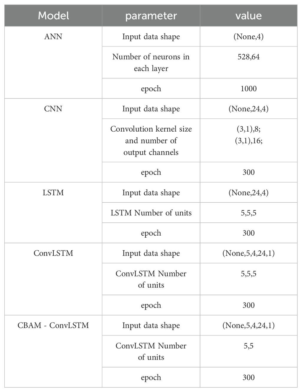
Table 1. Parameter settings for each model.

In addition to the hyperparameters listed in Table 1, some important parameter settings were consistent across the models. For instance, all models utilized the Adam optimizer, ReLU activation function, batch size of 256, and initial learning rate of 0.005 and employed the mean squared error (MSE) as the loss function during training. These settings were based on experimental findings and helped balance the training speed and forecast accuracy to a certain extent.

In addition to configuring the model structures and hyperparameters, it is essential to reformat the input data to satisfy the requirements of each model. Based on multiple experiments and relevant studies (Nitsure et al., 2014), the model inputs were determined as follows: ANN utilized the time series data from the previous 1 h; CNN and LSTM used the time series data from the previous 24 h; and ConvLSTM and CBAM-ConvLSTM utilized the time series data from the previous 120 h. These inputs were used to predict water levels at intervals of 6, 12, 24, and 48 h. During the training of the ANN, the input-output data pairs were offset according to the prediction step length. Short input data in models, such as CNN and LSTM, may prevent the model from learning underlying patterns within the forecast timescale, whereas excessively long inputs can reduce training efficiency and potentially degrade forecast accuracy compared with those of relatively shorter inputs. In certain cases, excessively long inputs may prevent the model from converging. Therefore, the choice of using the previous 24 h of time-series data as input strikes a balance between capturing sufficient temporal dependencies and maintaining the training efficiency for the CNN, LSTM, and similar models. For ConvLSTM and CBAM-ConvLSTM, which can efficiently handle longer input sequences, the input choice was aligned with the settings listed in Table 1.

Five prediction models were constructed for comparison. Figure 4 illustrates the schematic diagrams of each network structure used in this study. Specifically, the input data shapes for the models are as follows: the input tensor for the ANN is shaped as (None, 4); for the CNN and LSTM, it is shaped as a 3-dimensional tensor (None, 24, 4), where the first dimension represents the number of samples used in each training batch; the second dimension represents the length of the time series used in training; and the third dimension represents the number of channels indicating the input factors. The input data shape for CBAM-ConvLSTM and ConvLSTM is a 5-dimensional tensor, where the dimensions denote the number of samples used in each training batch, length of the time series used in training, number of channels, number of rows in the input data, and number of columns in the input data.

Figure 4

Figure 4. Architectures of the models used for prediction.

In this study, we forecast the measured water level 6h, 12h, 24h and 48h in advance respectively, and the output labeled data of the model are the measured water level after 6h, 12h, 24h and 48h respectively, and train the prediction model with different advance prediction lengths by setting up different inputs and labeled datasets respectively. All the models in this study were implemented using Python, primarily based on the PyTorch framework. To ensure reproducibility owing to the presence of randomness in the models, fixed random seeds were set for each model to guarantee reproducible results. After conducting multiple experiments, suitable parameter structures were determined, and the weights of each model were iteratively optimized.

4 Results and discussion

Table 2 shows the performance of each model in forecasting water levels 6, 12, 24, and 48 h ahead.

Table 2

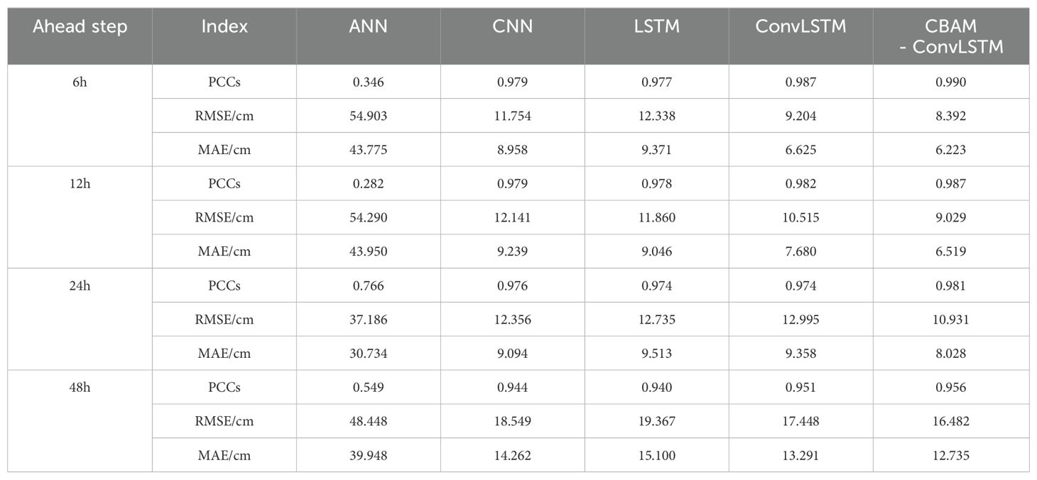
Table 2. Results of five models predicting multiple steps ahead on the test set.

Through a horizontal comparison of evaluation metrics among various models, it was observed that the CBAM-ConvLSTM model performed best across all multi-step-ahead forecasting and evaluation indicators. The ANN struggled to forecast the water-level trends in this experiment, exhibiting substantial overall errors. Across various forecast horizons, the CBAM-ConvLSTM model showed improvements compared to several baseline models. Specifically, the model reduced the average RMSE of each forecast horizon by approximately 21.2%, 19.2%, and 11.1% compared with those of LSTM, CNN, and ConvLSTM, respectively. The average MAE was reduced by approximately 23.2%, 20.6%, and 9.9% compared with those of the LSTM, CNN, and ConvLSTM, respectively. Overall, integrating the CBAM module shows the potential for enhancing model forecasting performance.

The prediction error of each model increased with an increase in the prediction step size, and CBAM-ConvLSTM exhibited the best performance. The comparison of various indices in the table demonstrates that the test set error of all models increases with an increase in the advanced prediction step size; however, compared with other baseline models, the CBAM-ConvLSTM model still has some advantages. Even when forecasting water levels 48 h in advance, the test set errors remained consistently low, indicating practical applicability.

To better compare the forecasting performance of each model, we analyzed the predictive capabilities of the CNN, LSTM, ConvLSTM, and CBAM-ConvLSTM models on a test set by plotting scatter diagrams. In Figure 5, the black line represents the polynomial fit of the predicted versus the actual values in the test set obtained using the least-squares method. The dashed black line corresponds to the y=x line. As the data density decreases, the colors of the scatter points in Figure 5 lighten, indicating that the data density is calculated using Gaussian kernel density estimation.

Figure 5

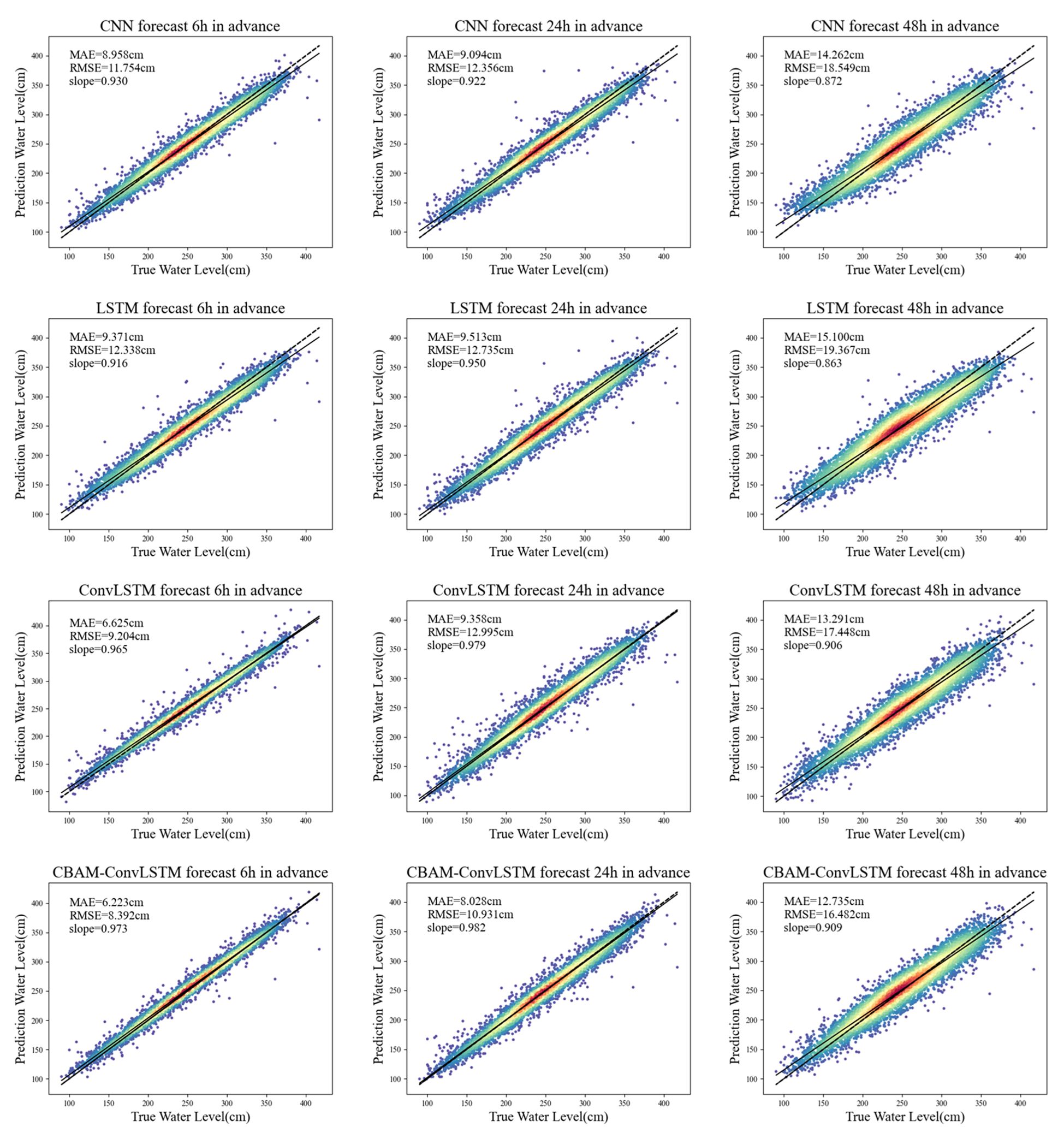
Figure 5. Scatter plots of water level forecasts 6, 24, and 48 h ahead using CNN, LSTM, ConvLSTM, and CBAM-ConvLSTM models.

A comparative analysis of the scatter distributions in Figure 5 reveals the superior performance of the CBAM-ConvLSTM model. Specifically, the model exhibited lower MAE and RMSE values. The overall data distribution is more concentrated and closer to the fitted line, with a smaller angle to the y=x line, indicating a closer alignment between the predicted and actual values. Compared with the other models, the CBAM-ConvLSTM model showed a more uniform distribution of forecast results around the fitted line. This characteristic became more pronounced with a longer prediction step size, suggesting a more reasonable distribution of the predicted values. Moreover, fewer scatter points significantly deviated from the fitted line compared to those in the other three models, further demonstrating the ability of the CBAM-ConvLSTM model to effectively forecast extreme events.

To visually assess the forecasting performance of each model, the predicted results of each model were compared with the actual water levels through visualization. Because of the large volume of data in the test set, which spans hourly data from April 3, 2020, to December 27, 2020, directly visualizing the forecast results does not easily reveal differences. Therefore, following the approach of Wang et al. (2021), the test set data were segmented, and the MAE was computed to obtain clearer results.

From Figure 6E, the performances of various models at different prediction step sizes in the test set show that the models proposed in this study generally outperform the other baseline models. CNN and LSTM exhibited increasing errors with longer prediction step sizes, whereas ConvLSTM and CBAM-ConvLSTM performed well, with the errors remaining within acceptable ranges. The distribution pattern of the MAE in the test set reveals larger errors in the latter half, coinciding with periods of frequent typhoons where station water levels are significantly influenced, resulting in weaker regularities and slightly larger forecasting errors. Comparing the latter half of the MAE values, the CBAM-enhanced ConvLSTM model shows smaller errors, indicating better learning of the hidden patterns in the data. Comparing the MAE distributions of the four prediction step sizes in Figures 6A–D, it is evident that, overall, the distributions are relatively uniform. In the latter half of the segments, the MAE of the model is relatively smaller compared to those of other models, particularly noticeable in the ahead 6-h forecast scenario, where the fluctuations in MAE in the test set are significantly reduced compared to those in other models. This observation validates the effectiveness of the proposed models.

Figure 6

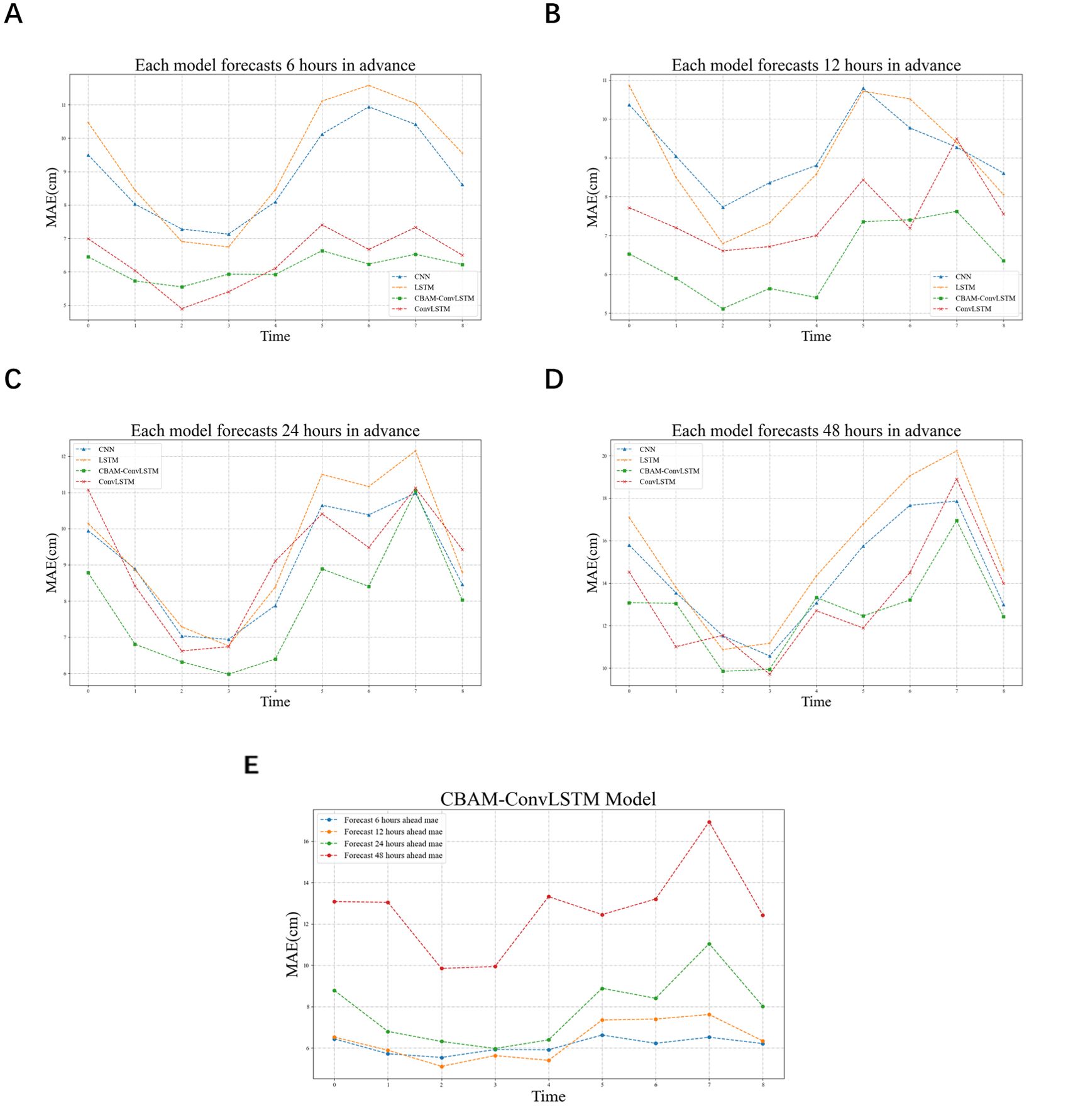
Figure 6. Segmental MAE comparisons of CNN, LSTM, ConvLSTM, and CBAM-ConvLSTM models forecasting 6 (A), 12 (B), 24 (C), and 48 (D) h ahead on the test set, and (E) segmental MAE comparisons of CBAM-ConvLSTM model forecasting 6, 12, 24, and 48 h ahead on the test set.

Nearshore water levels affected by typhoons often undergo drastic changes, typically resulting in storm surges. Accurately predicting such nonlinear and intense changes in water level can be challenging. This study used the Typhoon “Higos”, which passed near Zhuhai Station, as an example to further evaluate the forecasting capabilities of the models during typhoon events. Tropical Storm No. 2007 “Higos” formed in the northeast South China Sea on August 18, strengthened into a typhoon near the Guangdong coast at 20:00 on August 18, made landfall in Jinwan District, Zhuhai at 06:00 on August 19, then moved northwestward, weakened into a tropical depression after entering Guangxi, and was stopped numbering by the Central Meteorological Observatory at 23:00 on August 19.

Figures 7A–D show the forecasted and actual water level changes at 6, 12, 24, and 48 h ahead. It is evident that as the prediction step size increases, the forecast performance of all models gradually decreases. However, overall, the CBAM-ConvLSTM model performs relatively well. During typhoon “Higos”, compared to CNN, LSTM, and ConvLSTM models, the CBAM-ConvLSTM model reduces the average MAE by approximately 15.5%, 19.2%, and 10.5%, respectively, at various prediction steps. Specifically, compared to other top-performing models, the CBAM-ConvLSTM model reduces MAE by approximately 3.2 and 2.4 cm at 6 and 24h forecasting steps, respectively, representing reductions of approximately 18% and 11% in forecast errors. As the prediction step size increases, forecasting difficulty also increases accordingly, yet the CBAM-ConvLSTM model maintains relatively low errors, demonstrating the effectiveness of the attention module.

Figure 7

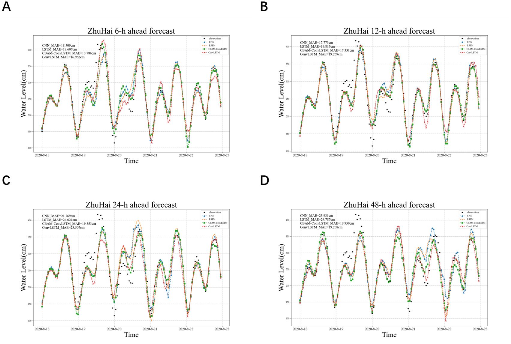
Figure 7. Forecasted and actual water levels by CNN, LSTM, ConvLSTM, and CBAM-ConvLSTM models at 6 (A), 12 (B), 24 (C), and 48 (D) h ahead during Typhoon “Higos”.

During August 19, the tidal stations were substantially affected by typhoons, resulting in abnormally high-water levels. All models underestimated the water-level rise caused by storm surges; however, the potential for improved water-level forecasting capability was evident in the CBAM-ConvLSTM model. The CNN and LSTM models showed poor sensitivity to short-term storm surges, underestimated their impact, and consistently overestimated normal water levels post-storm surges. Compared to CBAM-ConvLSTM, ConvLSTM exhibited less stability, slightly lagging in forecasting some high tide water levels on August 19 at a 6 h forecasting step, and underestimating the water levels on August 19 and August 22 at 24 and 48 h forecasting steps compared to other models. Across all prediction step sizes, CBAM-ConvLSTM performed relatively well in forecasting abnormally high-water levels from August 19 to August 20, closely matching the actual water levels. This indicates that the CBAM-ConvLSTM model effectively captures the impacts of typhoon events, demonstrating its advantages in storm surge prediction tasks.

However, the CBAM-ConvLSTM model exhibited certain limitations, with a noticeable decline in performance when forecasting over an extended prediction step size. As demonstrated in Figure 8, the CBAM-ConvLSTM model achieved the highest accuracy in 6-h advance forecasts. However, as the prediction step size for advanced forecasts increased, the ability of the model to predict anomalous water levels gradually diminished. At a 48-h forecasting step, although the fit of the model is superior to that of other models, it still tends to underestimate some extreme water levels. The primary pattern the model has mainly learned is tidal variation, and it struggles to further learn the nonlinear patterns brought about by typhoons, which is also a current challenge in extending the prediction step size. There are two possible reasons for this finding. First, training data selection may not be sufficiently comprehensive. Although this study used water level, wind, and precipitation data as the training and validation data of the model, these few factors and data from a single station may not fully reflect the characteristics of coastal water level changes. The potential patterns learned by the model are limited, making it difficult to maintain the forecasting capabilities over longer prediction step sizes. Second, there is an issue with the model and its structures. The CBAM and ConvLSTM models used in this study have certain advantages in handling such time-series data; however, with the rapid development of various model algorithms, there may be models and modules that are more suitable for this issue. Moreover, the structure of the model in this study is a relatively lightweight architecture determined after experimentation and may not be the optimal solution. There is still room for improvement in the structure of the model. However, the CBAM-ConvLSTM model proposed in this study for predicting water levels remains a potential model for water level forecasting.

Figure 8

Figure 8. Forecasted and actual water levels by CBAM-ConvLSTM model at 6, 12, 24, and 48 h ahead during Typhoon “Higos”.

5 Conclusion

The primary focus of this study is a comparative analysis of the CBAM-ConvLSTM model, which incorporates an attention mechanism, with models such as an artificial neural network (ANN), convolutional neural network (CNN), long short-term memory (LSTM), and ConvLSTM, in the context of water level forecasting at the Zhuhai station. The CBAM-ConvLSTM model, through its convolutional block attention module (CBAM), can focus on considerable features within the data, enhancing their importance, and thus better identifying anomalous events in water-level data compared to other models. Additionally, by integrating the ConvLSTM model, it effectively learns the multiscale characteristics of the data, leading to superior forecasting outcomes. Furthermore, to achieve a model that consumes minimal computational resources while maintaining relatively high forecasting accuracy, all model structures and parameter settings in this study were determined through multiple experimental adjustments.

The CBAM-ConvLSTM model demonstrated superior performance in the water-level prediction task at Zhuhai Station compared with those of the other four baseline models used for comparison. The model showed higher accuracy in short-term forecasts than that in long-term forecasts and was capable of effectively forecasting water levels 48 h in advance. On average, the CBAM-ConvLSTM model improved the performance by approximately 20% on the test set compared with those of the CNN and LSTM models. When the CBAM module was incorporated into the model, the performance on the test set improved by approximately 10% compared to that of the ConvLSTM model. During typhoon “Higos”, the model reduced the mean absolute error (MAE) by approximately 3.2 and 2.4 cm for the 6- and 24-h forecasts, respectively, which corresponds to a reduction of approximately 18% and 11% in forecasting error. Across the four prediction step sizes, the performance of the model improved by approximately 10%, showing better forecasting capabilities for storm surges compared to those of the other baseline models, and thus holding a certain practical value.

The model used in this study is also applicable for forecasting at other tidal stations, provided sufficient data are available. Nevertheless, there are some areas where our study falls short:(1) The more comprehensive and reliable set of factors affecting nearshore water levels for forecasting. Because there is a certain interplay between the water level variations at coastal stations and the various influencing factors, combining various effective factors can reveal hidden features, which can contribute to better forecasting outcomes. (2) Optimizing model parameter structures to extend the prediction step size. The parameter structure determined in this study may not be the best solution; other structures may consume fewer computational resources and yield better forecasting results.

Data availability statement

The original contributions presented in the study are included in the article/Supplementary Material. Further inquiries can be directed to the corresponding author.

Author contributions

JY: Conceptualization, Data curation, Formal analysis, Methodology, Software, Visualization, Writing – original draft. TZ: Conceptualization, Data curation, Formal analysis, Funding acquisition, Project administration, Resources, Supervision, Writing – review & editing. JZ: Data curation, Writing – review & editing. XL: Writing – review & editing. HW: Writing – review & editing. TF: Writing – review & editing.

Funding

The author(s) declare financial support was received for the research, authorship, and/or publication of this article. This research was jointly funded by independent research project of Southern Ocean Laboratory (Grant number SML2022SP301); National Natural Science Foundation of China (Grant number 42476219); National Natural Science Foundation of China (Grant number 41976200); Innovative Team Plan for Department of Education of Guangdong Province (No. 2023KCXTD015); National Key Research and Development Program of China (Grant number 2022YFC3103104, 2021YFC3101801); Guangdong Science and Technology Plan Project (Observation of Tropical marine environment in Yuexi); Guangdong Ocean University Scientific Research Program (Grant number 060302032106).

Conflict of interest

The authors declare that the research was conducted in the absence of any commercial or financial relationships that could be construed as a potential conflict of interest.

Publisher’s note

All claims expressed in this article are solely those of the authors and do not necessarily represent those of their affiliated organizations, or those of the publisher, the editors and the reviewers. Any product that may be evaluated in this article, or claim that may be made by its manufacturer, is not guaranteed or endorsed by the publisher.

Supplementary material

The Supplementary Material for this article can be found online at: https://www.frontiersin.org/articles/10.3389/fmars.2024.1470320/full#supplementary-material

References

Bengio Y., Simard P., Frasconi. P. (1994). Learning long-term dependencies with gradient descent is difficult. IEEE Trans. Neural Networks 5, 157–166. doi: 10.1109/72.279181

Crossref Full Text | Google Scholar

Corbetta M., Shulman G. L. (2002). Control of goal-directed and stimulus-driven attention in the brain. Nat. Rev. Neurosci. 3, 201–215. doi: 10.1038/nrn755

PubMed Abstract | Crossref Full Text | Google Scholar

El-Diasty M., Al-Harbi S., Pagiatakis S. (2018). Hybrid harmonic analysis and wavelet network model for sea water level prediction. Appl. Ocean Res. 70, 14–21. doi: 10.1016/j.apor.2017.11.007

Crossref Full Text | Google Scholar

Hersbach H., Bell B., Berrisford P., Biavati G., Horányi A., Muñoz Sabater J., et al. (2023). Data from: ERA5 hourly data on single levels from 1940 to present. Copernicus Climate Change Service (C3S) Climate Data Store (CDS). doi: 10.24381/cds.adbb2d47

Crossref Full Text | Google Scholar

Hochreiter S., Schmidhuber J. (1997). Long short-term memory. Neural Comput. 9, 1735–1780. doi: 10.1162/neco.1997.9.8.1735

PubMed Abstract | Crossref Full Text | Google Scholar

Hu J., Shen L., Sun G. (2018). “Squeeze-and-excitation networks,” in 2018 IEEE/CVF Conference on Computer Vision and Pattern Recognition. Salt Lake City, UT, USA, 7132–7141. doi: 10.1109/CVPR.2018.00745

Crossref Full Text | Google Scholar

Itti L., Koch C., Niebur E. (1998). A model of saliency-based visual attention for rapid scene analysis. IEEE Trans. Pattern Anal. Mach. Intell. 20, 1254–1259. doi: 10.1109/34.730558

Crossref Full Text | Google Scholar

Jalalifar R., Delavar M. R., Ghaderi S. F. (2024). SAC-ConvLSTM: A novel spatio-temporal deep learning-based approach for a short term power load forecasting. Expert Syst. Appl. 237, 121487. doi: 10.1016/j.eswa.2023.121487

Crossref Full Text | Google Scholar

Kagemoto H. (2020). Forecasting a water-surface wave train with artificial intelligence- A case study. Ocean Eng. 207, 107380. doi: 10.1016/j.oceaneng.2020.107380

Crossref Full Text | Google Scholar

Larochelle H., Hinton G. (2010). Learning to combine foveal glimpses with a third-order Boltzmann machine. Adv. Neural Inf. Process. Syst. 23, 1243–1251. doi: 10.5555/2997189.2997328

Crossref Full Text | Google Scholar

LeCun Y., Bottou L., Bengio Y., Haffner P. (1998). Gradient-based learning applied to document recognition. Proc. IEEE 86, 2278–2324. doi: 10.1109/5.726791

Crossref Full Text | Google Scholar

McCulloch W. S., Pitts W. (1943). A logical calculus of the ideas immanent in nervous activity. Bull. Math. biophysics 5, 115–133. doi: 10.1007/BF02478259

Crossref Full Text | Google Scholar

Mel R., Viero D. P., Carniello L., Defina A., D’Alpaos L. (2014). Simplified methods for real-time prediction of storm surge uncertainty: The city of Venice case study. Adv. Water Resour. 71, 177–185. doi: 10.1016/j.advwatres.2014.06.014

Crossref Full Text | Google Scholar

Nitsure S. P., Londhe S. N., Khare K. C. (2014). Prediction of sea water levels using wind information and soft computing techniques. Appl. Ocean Res. 47, 344–351. doi: 10.1016/j.apor.2014.07.003

Crossref Full Text | Google Scholar

Ouyang L., Ling F., Li Y., Bai L., Luo J. J. (2023). Wave forecast in the Atlantic Ocean using a double-stage ConvLSTM network. Atmospheric Oceanic Sci. Lett. 16, 100347. doi: 10.1016/j.aosl.2023.100347

Crossref Full Text | Google Scholar

Shi X., Chen Z., Wang H., Yeung D. Y., Wong W. K., Woo W. C. (2015). Convolutional LSTM network: A machine learning approach for precipitation nowcasting. Adv. Neural Inf. Process. Syst. 28, 802–810. Available at: http://arxiv.org/abs/1506.04214.

Google Scholar

Sztobryn M. (2003). Forecast of storm surge by means of artificial neural network. J. Sea Res. 49, 317–322. doi: 10.1016/S1385-1101(03)00024-8

Crossref Full Text | Google Scholar

Vaswani A., Shazeer N., Parmar N., Uszkoreit J., Jones L., Gomez A. N., et al. (2017). Attention is all you need. Adv. Neural Inf. Process. Syst. 30, 6000–6010. doi: 10.48550/arXiv.1706.03762

Crossref Full Text | Google Scholar

Wang B., Liu S., Wang B., Wu W., Wang J., Shen D. (2021). Multi-step ahead short-term predictions of storm surge level using CNN and LSTM network. Acta Oceanologica Sin. 40, 104–118. doi: 10.1007/s13131-021-1763-9

Crossref Full Text | Google Scholar

Woo S., Park J., Lee J. Y., Kweon I. S. (2018). “CBAM: Convolutional block attention module,” in Proceedings of the European conference on computer vision (ECCV). 3–19. Available at: http://arxiv.org/abs/1807.06521.

Google Scholar

Yang C.-H., Wu C.-H., Hsieh C.-M. (2020). Long short-term memory recurrent neural network for tidal level forecasting. IEEE Access, 8, 159389–159401. doi: 10.1109/ACCESS.2020.3017089

Crossref Full Text | Google Scholar

Zhang X., Wang T., Wang W., Shen P., Cai Z., Cai H. (2023). A multi-site tide level prediction model based on graph convolutional recurrent networks. Ocean Eng. 269, 113579. doi: 10.1016/j.oceaneng.2022.113579

Crossref Full Text | Google Scholar

Zhao X., Jiang N., Liu J., Yu D., Chang J. (2020). Short-term average wind speed and turbulent standard deviation forecasts based on one-dimensional convolutional neural network and the integrate method for probabilistic framework. Energy Conversion Manage. 203, 112239. doi: 10.1016/j.enconman.2019.112239

Crossref Full Text | Google Scholar

Zhou S., Xie W., Lu Y., Wang Y., Zhou Y., Hui N., et al. (2021). ConvLSTM-based wave forecasts in the South and East China seas. Front. Mar. Sci. 8. doi: 10.3389/fmars.2021.680079

Crossref Full Text | Google Scholar