Comprehensive comparative analysis of reconstructed sea level datasets in the China Seas: insights from tide gauge and satellite altimetry

At present, there are many reconstructed datasets at the global scale. To test the applicability of these datasets in the China seas, the study comprehensively analyzes the reliability and accuracy of reconstructed sea level datasets in capturing nuanced temporal patterns of sea level changes in the China Seas. This study applied analysis methods or indicators such as time series, Taylor plots, correlation coefficients, growth rates, and standard deviations. Ocean Data Assimilations (ODAs) outperform Tide Gauge Reconstructions (TGRs) in terms of correlation with measured data in the nearshore, while TGRs exhibit superior capability in capturing oceanic sea level variability. Although the ODAs and TGRs both suffer from the underestimation of sea level variability in China as well as in neighboring seas, the TGRs perform better than the former. ODAs show inconsistency in reflecting the rate of sea level rise, but they, particularly the China Ocean Reanalysis (CORA), demonstrate a better correlation with satellite altimetry datasets. Meanwhile, both of them can reflect the Pacific Decadal Oscillation (PDO) well. TGRs, relying on oceanic tide gauge stations, suffer from poor correlation with tide gauge stations due to limited coverage. Reconstruction discrepancies are attributed to methodological differences and data assimilation techniques. Future studies should explore alternative variables like sea surface temperature and so on to enhance sea-level reconstruction, especially in regions with sparse tide gauge coverage.

1 Introduction

Sea level rise has profound implications for coastal societies, island nations, and the global population and economy. Consequently, comprehending sea level changes in response to climate change stands as one of the most critical issues for climate scientists (Milne et al., 2009; Church et al., 2011; Han et al., 2017; Horton et al., 2020). Sea level measurement has long been a pivotal component of oceanographic surveys. Tide gauges and satellite altimetry represent the most prevalent approaches for sea level measurements. Tide gauges offer detailed and long-term sea level information at a temporal scale; however, they are constrained by uneven geographical distribution, inconsistent observation, a lack of uniform reference level, and unsuitability for deep-sea measurements, making studies of large-scale patterns of ocean variability difficult (Cipollini et al., 2017; Adebisi et al., 2021).

Since 1993, satellite altimetry has played a pivotal role in providing precise measurements of sea surface height and comprehensive coverage across the globe. This technological advancement significantly enhances the accuracy of our observations and deepens our understanding of sea level dynamics (Leuliette et al., 2004; Beckley et al., 2007; Nerem et al., 2010; Chen et al., 2017; Hamlington et al., 2019; Horton et al., 2020; Zhou et al., 2022; Guérou et al., 2023). However, satellite data only offer oceanic information after 1993, and with the modern altimetry record spanning a mere 30 years, comprehending lower-frequency signals known to exist in the ocean remains a challenge (Hamlington et al., 2016, 2019).

In response to the disadvantages of tidal gauge and satellite data, numerous studies have been undertaken over recent decades. Since 2002, a method integrating the extensive time-series data obtained from Tidal Gauge (TG) stations with the spatial covariance information of sea level derived from satellite altimetry has been widely employed for the reconstruction of historical sea level fields (Chambers et al., 2002; Church et al., 2004; Church and White, 2006; Church et al., 2011; Ray and Douglas, 2011; Hamlington et al., 2012a; Hay et al., 2015; Kumar et al., 2020; Mu et al., 2024). The empirical orthogonal function (EOF) and cyclostationary empirical orthogonal function (CSEOF) have emerged as the predominant techniques utilized in sea level reconstructions. Another approach is the ocean reanalysis, generated through ocean models driven by atmospheric reanalysis and constrained by historical ocean observations. Several extant ocean reanalysis products are now available for the investigation of global decadal sea level variability (Carton and Giese, 2008; Zuo et al., 2019). On a global scale, Carson et al. (2017) conducted a comparative analysis of several extant statistical and dynamical reconstructions with tide gauges spanning from 1960 to 2007. Their findings revealed significant deviations among all products in terms of decadal variability and trends, highlighting pronounced spatial disparities. Although sea level is a global phenomenon, regional deviations from the global mean trend frequently exceed 50-100%, particularly along the coastlines of the Pacific Ocean (Han et al., 2011; Hamlington et al., 2018). Consequently, the primary objective of this study is to reassess the reliability of existing statistical and dynamical reconstructions at local or regional levels.

In this study, our focus is on the China Sea, encompassing the Bohai Sea, the Yellow Sea, the East China Sea, and the South China Sea. These regions were identified as among the most susceptible areas under climate change scenarios (Hallegatte et al., 2013), however, the number of tide gauges is very limited around the China Seas compared to regions like North America and Europe (Fang et al., 2021; Feng et al., 2023). Utilizing data from tide gauges and satellite altimetry, numerous investigations have explored the regional sea level variability in the China Seas through statistical and dynamical reconstructions (Cheng et al., 2015; Cheng et al., 2016; Feng et al., 2015; Guo et al., 2015; Strassburg et al., 2015; Liu et al., 2020, 2023). Also, since 2011 the National Marine Data and Information Service (NMDIS) has developed the China Ocean Reanalysis (CORA) system for coastal waters of China and adjacent seas (Han et al., 2011, 2013a, b). It is imperative to assess the performance of these reconstructions to ensure the reliability of research outcomes.

The structure of the paper is as follows: The data and method section are concise overviews of the investigated data products, emphasizing notable distinctions. The results section is subdivided into various subsections based on distinct characteristics, including correlation and long-term trends. The conclusion section comprises concluding remarks and recommendations.

2 Data and methodology

2.1 Data

The Datasets involved in this study have some reconstruction products, the tide gauge data, and satellite altimetry data. To compare the strengths and weaknesses of reconstructions in representing sea level variations on the China Seas, we have standardized the research region (0°N-50°N, 100°E-140°E) for all datasets. To compare satellite altimetry era and long-term variables, the period studied is split into two parts: the whole period of 1960–2008 and the altimetry period of 1993–2008. This time range is a common interval for almost all data.

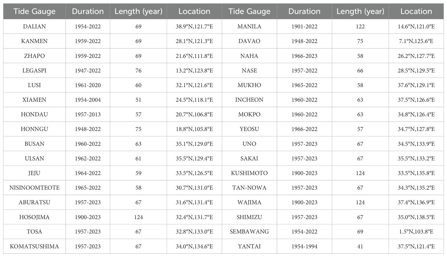
The tide gauge data containing monthly mean sea level records of 32 tide gauges (Figure 1) is collected from the Permanent Service for Mean Sea Level (PSMSL). Tide gauges can only be established on land, resulting in significant spatial limitations in data distribution (Hamlington et al., 2011; Sheng, 2016). For instance, there are hardly any tide gauges in the South China Sea and the open waters of the Pacific Ocean. See Figure 1 for the research region and specific distribution of tide gauges.

Figure 1

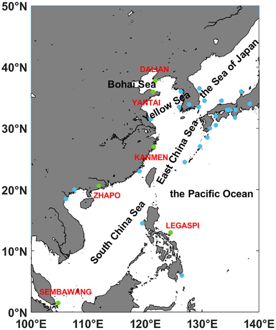
Figure 1. The research region and distribution of tide gauges. The tide gauges marked in green are those mentioned in Figure 3, while the blue pots are other important stations not mentioned in Figure 3.

One crucial criterion for selecting tide gauges is that their temporal span must be long enough. To get more data, the tide gauge data having slight discrepancies with the period are optimized by using interpolation and are also used to evaluate the products. Taking Dalian as an example, linear interpolation is used to fill in the missing data from 1958 to 1967. The model-based Glacial Isostatic Adjustment (GIA) from Bing and Qiang, (2018) is employed to correct tide gauge records from Vertical movement of land. See Table 1 for a summary of the tide gauges’ temporal information.

Table 1

Table 1. A summary of the tide gauges’ temporal information.

As another validation data, the satellite altimetry data is obtained from the Archiving, Validation, and Interpretation of Satellite Oceanographic (AVISO) quarter-degree-resolution, multiple altimeter monthly product. This dataset integrates information from several altimetry satellites, including Jason-1, T/P, Envisat, GFO, ERS-1/2, and GEOSAT. The spatial grid resolution is 1/4°×1/4°, and the temporal resolution involves month-by-month averaging. The temporal scope of this analysis spans from January 1993 to December 2020.

The products requiring validation are categorized as reconstructions derived from statistical tide gauges (TGR) and dynamical ocean reanalysis, also known as ocean data assimilation (ODA). The TGRs encompass the CSIRO product and CCAR product. The CSIRO product represents an improvement of the original dataset outlined in Church et al. (2004), with the new iteration extended up to 2012. The fundamental loading patterns correspond to a subset of global EOF derived from altimetry data, capturing the predominant Sea Surface Height (SSH) variability. Subsequently, these patterns are regressively fitted to a curated selection of tide gauges through a least squares approach to yield the reconstructed SSH fields. The reconstruction methodology employed by CCAR follows a similar approach to the CSIRO product, albeit with a distinct feature. Instead of utilizing conventional EOFs derived from altimetry data, CCAR incorporates CSEOF as proposed by Hamlington et al. (2011; 2012b). These CSEOFs exhibit variability with a defined periodicity, thereby capable of representing cyclic phenomena such as the annual cycle within a singular mode. Since CCAR data is weekly averaged, we utilize a simple three-dimensional interpolation method to convert it into monthly data.

The ODAs include ORAS5 (Ocean Reanalysis System 5), Simple Ocean Data Assimilation (SODA v2.2.4) datasets, and the China Ocean Reanalysis version 1.0 datasets (CORA v1.0). The ORA-S5 dataset is developed by the European Centre for Medium-Range Weather Forecasts (ECMWF) within the OCEAN5 ocean analysis system. This system is composed of 5 ensemble members and employs the 3D-Var FGAT (First Guess at Appropriate Time) assimilation technique, which integrates sub-surface temperature, salinity, sea-ice concentration, and sea-level anomalies. Covering the period from 1979 to the present, with an additional backward extension from 1958 to 1978, the data is characterized by a spatial resolution of 1° × 1°.

SODA v2.2.4 is available for download from the IRI/LDEO Climate Data Library (Giese and Ray, 2011). This dataset is constructed based on the Parallel Ocean Program physics, featuring an average resolution of 0.25° × 0.25° × 40 levels (Smith et al., 1992). It assimilates a comprehensive range of observational data sources, including hydrographic profiles, ocean station data, moored temperature and salinity time series, various surface temperature and salinity observations, and satellite data. Representing the period from 1871 to 2008, this version marks the inaugural assimilation run by the authors spanning over a century.

CORA v1.0 was downloaded from the National Marine Data Center (http://mds.nmdis.org.cn/). The ocean dynamical model utilized in CORA v1.0 is the Princeton Ocean Model with a generalized coordinate system (POMgcs). It incorporates the multigrid three-dimensional variational (3D-Var) ocean data assimilation method, which was developed by NMDIS (Li et al., 2006). The assimilated observations encompass in-situ profiles, altimeter sea level anomaly (SLA), satellite sea surface temperature (SST), and TPXO8 (TOPEX/POSEIDON global tidal model) surface tidal elevation. This dataset spans the period from 1958 to 2021, with a spatial resolution of 0.5° × 0.5°. Additionally, you can access the PDO index at http://jisao.washington.edu/pdo/PDO.latest. See Table 2 for a summary of every reconstruction.

Table 2

Table 2. A summary of every reconstruction’s information.

2.2 Method

It is important to note that sea level reconstructions and models do not necessarily depict the same sea level. Sea level reconstructions rely on data from tide gauges, which encompass land ice melt and additional ocean mass variations, including land water storage, in their sea level estimates (Church et al., 2004; Peltier, 2004). The removal of the temporal mean value from all datasets, and the tide gauges used for comparison (refer to below), addresses a significant portion of the issues related to ice mass loss and landwater storage (Carson et al., 2017).

In the period of our study, tide gauge data served as the reference for the computation of correlations between tide gauge data and datasets from distinct products at 32 specified locations. The methodology encompassed the utilization of the nearest neighbor interpolation technique to procure data from different products. Subsequently, a comparative analysis was conducted at 6 selected tide gauge locations to elucidate the similarities and disparities between the tide gauges’ time series and those of the various products through line graphs. Furthermore, a quantitative assessment of the correlations and standard deviations between these time series was performed utilizing Taylor diagrams. Lastly, we will juxtapose the growth rates of tide gauge data with those of various products on the same coordinate system to highlight their trend discrepancies.

Using satellite altimetry data as a reference, we compared the annual mean time series of satellite altimetry data with various product data using line plots. During the above process, we used the formula (Sheng, 2016) below to calculate the spatial average mean:

$\begin{array}{ll}\overline{{\mathit{\text{h}}}_{\mathit{\text{k}}}}=\frac{{\displaystyle {\sum }_{\mathit{\text{i}}}{\displaystyle {\sum }_{\mathit{\text{j}}}{\mathit{\text{h}}}_{\mathit{\text{ijk}}}}}\mathbf{\text{cos}}({\mathit{\text{φ}}}_{\mathit{\text{j}}})}{{\displaystyle {\sum }_{\mathit{\text{i}}}{\displaystyle {\sum }_{\mathit{\text{j}}}\mathbf{\text{cos}}}({\mathit{\text{φ}}}_{\mathit{\text{j}}})}}& (1)\end{array}$

In Equation 1, $\overline{h_k}$: the regional average at time point k; i, j: the geographical location of the grid point; $h_{ijk}$: the data value for the geographical location (i, j) at time point (k); and ${\phi }_j$: the latitude of the grid point.

The correlation coefficients between satellite altimetry data and various product data at each point were computed. To account for the dissimilarities in spatial resolutions between datasets, a three-dimensional interpolation method was employed to reconcile the grid of satellite altimetry data with that of the various product datasets. Furthermore, the growth rates for all grid points of both the satellite altimetry data and the various product datasets were calculated and depicted on a large-scale map to visualize the trend of each product during the satellite altimetry era. Lastly, the standard deviation of each grid data of satellite altimetry data and other product data was employed to reflect the interdecadal variability. The standard deviation that commonly used to evaluating low-frequency variability in datasets (Barnston and van den Dool, 1993; Manabe and Stouffer, 1996; Dubrovský et al., 2004) quantifies the extent of data dispersion, is robust against noise, facilitates comparative analysis. Additionally, the correlations between the PDO index and various products including satellite data were explored to illuminate the influence of the PDO on sea level.

3 Results

3.1 Time series

Figure 2 depicts the annual mean sea level and satellite altimetry time series for all datasets in the East China Sea (Figure 2A, including the Bohai Sea, the Yellow Sea, and the East China Sea) and the South China Sea (Figure 2B). All datasets show clear decadal variations and upward trends. Satellite data show that the sea level rise trend in the East China Sea between 1993 and 2020 is about 4.44 ± 0.23 mm/year and that in the South China Sea is about 4.6 ± 0.34 mm/year. Among them, in the East China Sea, the sea level rise trend of all datasets is slower than that of the satellite altimetry data, while in the South China Sea, the CSIRO dataset has a rise trend of 5.34 ± 0.22 mm/year, which is beyond the trend of satellite altimetry. The CCAR trend is very close, at 3.33 ± 0.13 mm/year in the East China Sea and 4.01 ± 0.35 mm/year in the South China Sea. While the CORA trend is much lower, less than half that of the satellite data, at 0.58 ± 0.21 mm/year in the East China Sea and 1.83 ± 0.33 mm/year in the South China Sea. And the trend of CORA between 1958 and 2008 is even negative. Taking the East China Sea as an example, the time series of CORA has undergone MK trend testing, and obtained a statistic Z of -1.8356, which confirms the rationality of the negative growth rate in Figure 2A. Despite marked distinctions among the restructured products, some areas of consistency persist. All datasets indicate a rising trend in total sea level across the China Seas. Generally, sea level exhibited slow growth before the altimetry era (1958-1993), transitioning thereafter into a phase of rapid escalation.

Figure 2

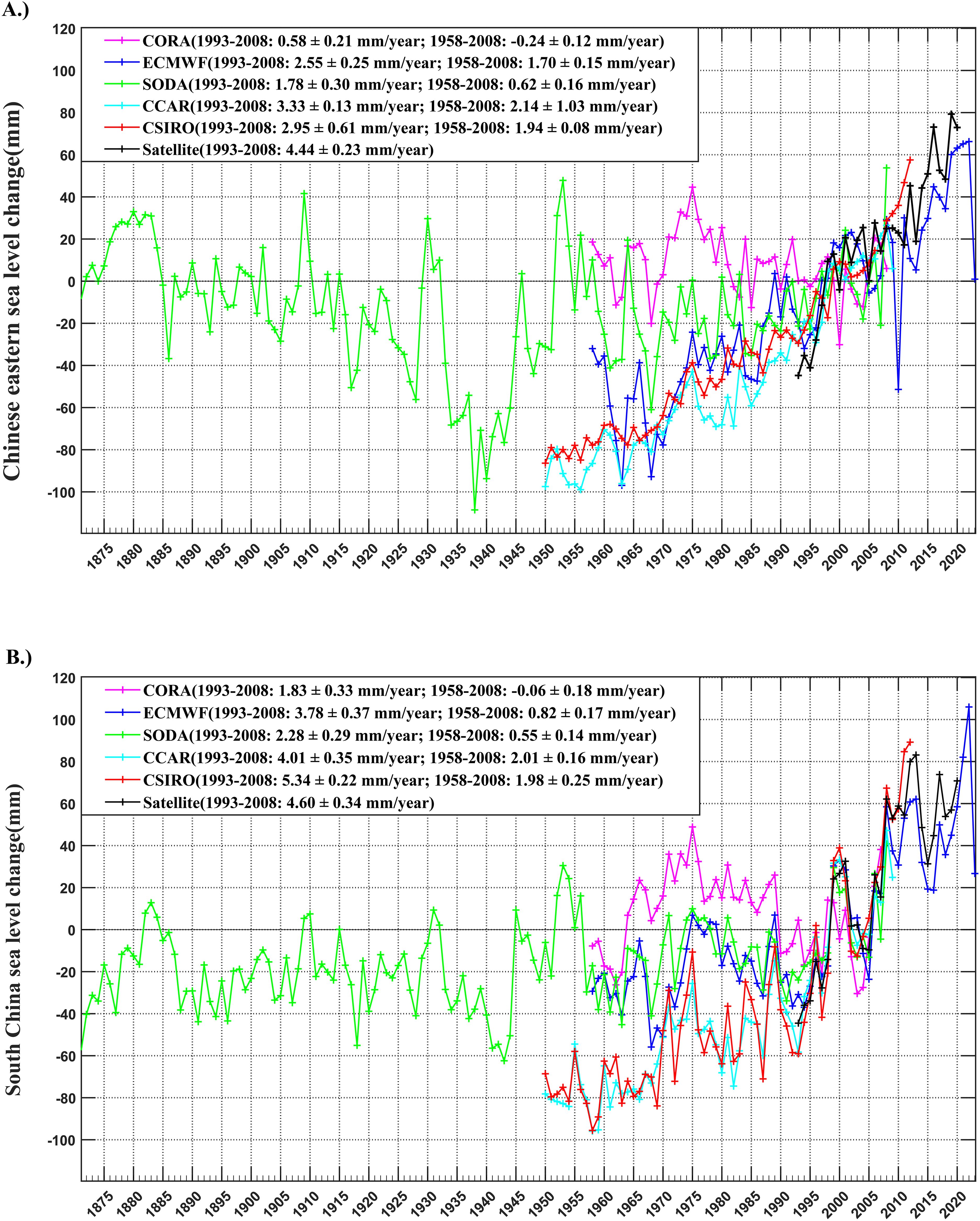
Figure 2. Time series of regional average sea level anomaly. [A: The East China Seas (115.5-131.5°E, 21.5-42.0°N) ; B: The North China Sea (103.5-122.5°E, 1.5-24.5°N)].

3.2 Compared to tide gauge data

The time series of all reconstructions were compared with data provided from multiple tide gauge locations, as depicted in Figure 3. The results indicated that there were some discrepancies between the tide gauges and various data products. Generally, the reconstructions aligned more closely with the variability observed in tide gauges at KANMEN, ZHAPO, and SEMBAWANG. In the case of YANTAI, data from all products from 1972 to 1990 exhibited higher values than those recorded by the tide gauge. At LEGASPI, except for CORA, other products consistently underestimated the increasing trend throughout the period. CORA displayed a pronounced mutation, indicating that before 2008, the data exhibited less variability compared to the tide gauge data across nearly all stations. Nonetheless, both inter-annual and decadal variability saw an increase. Compared to other products, the ECMWF, SODA, and CCAR data sets demonstrated a better match with the variability of the tide gauges (refer to Figures 3A, B, E, F for examples). Among them, the increase trend of CSIRO is very stable, with minimal data oscillation. At six tide gauge stations, the SODA data significantly underestimated the increasing trend, particularly at Legaspi.

Figure 3

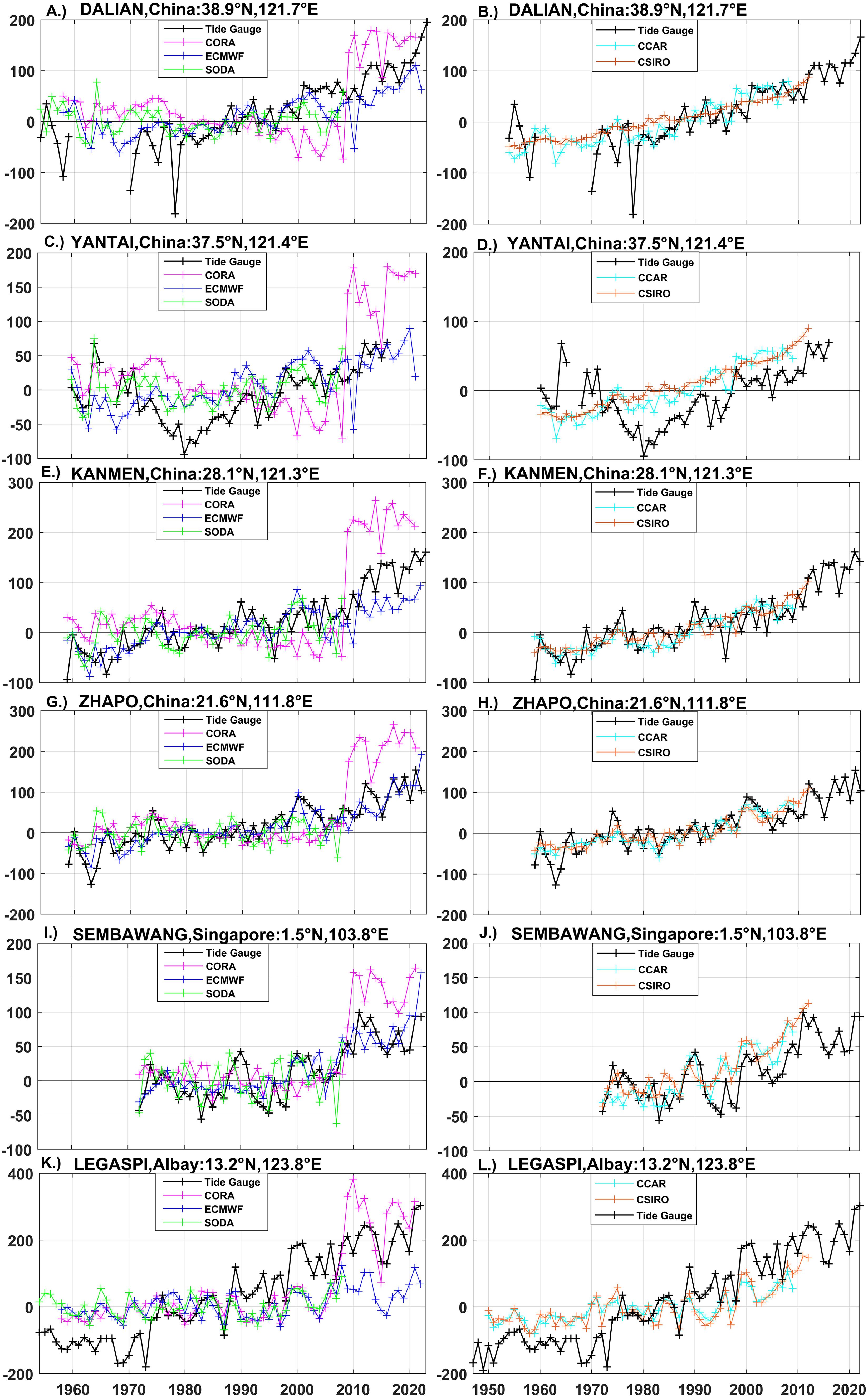
Figure 3. The 6 representative tide gauges (black) are compared with interpolations at this tide gauge calculated from the ODAs (A, C, E, G, I, K) and the TGRs (B, D, F, H, J, L).

Furthermore, the Taylor diagram of the annual mean SSH of the 5 datasets is presented in Figure 4. Generally, the correlation between each product and the tide gauge is not high. It can be seen that the correlation of CCAR datasets at the tide gauge stations of DALIAN (refer to Figure 4A)/YANTAI (refer to Figure 4B)/ZHAPO (refer to Figure 4D)/SEMBAWANG (refer to Figure 4E) are more than 0.5, and the standard deviation is less than 0.5, which shows a better performance compared with other sets of datasets. The SODA dataset also performs well at two tide gauge stations, YANTAI and ZHAPO, meanwhile, CORA performs excellently at the KANMEN (refer to Figure 4C) site but not so well at several other tide gauge stations. Tide gauges at stations ZHAPO/SEMBAWANG, each reconstructed dataset has a good performance. In ZHAPO, the correlation of each dataset is greater than 0.5, and the standard deviation is less than 0.4; and in SEMBAWANG, the correlation of each dataset is greater than 0.5, and the standard deviation is less than 0.6, except for CORA. Another, the root mean square errors (RMSE) for all products are not ideal overall, mostly exceeding 0.8. Particularly at LEGASPI, all RMSE values are above 2 (refer to Figure 4F). In summary, CCAR performs optimally in these five datasets when compared to the six tide gauge stations selected in this paper.

Figure 4

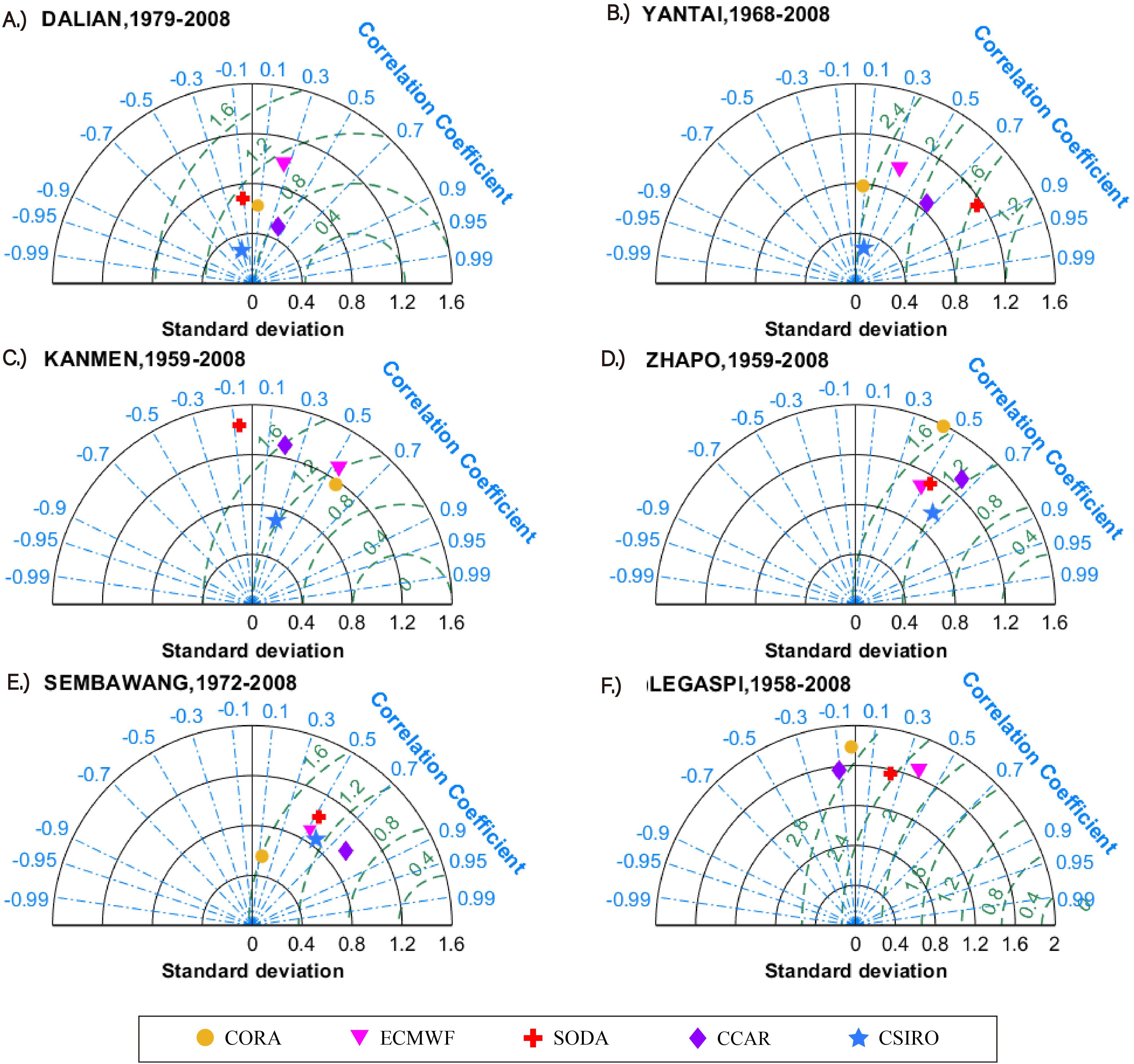
Figure 4. Taylor diagram of the annual mean SSH of 5 datasets compared to the observation data of 6 tide gauges (A–F: Different tide gauge stations).

The correlation between tide gauges and every product is displayed in Figure 5. It’s notable that compared to the TGR (CCAR, CSIRO), the ODAs (CORA, ECMWF, SODA) show a higher correlation with close to 80% of the stations reaching a correlation of 0.7 and above. The correlation with tide gauge stations in all three ODAs datasets is 0.8 and above for six sites including DALIAN, NASE, NISINOOMOTE, SAKAI DAVAO, and SEMBAWANG. However, both CORA and ECMWF (Figures 5A, B) have correlations with MUKHO stations below 0.1, in contrast, the SODA dataset (Figure 5C) has a better correlation with tide gauge stations among the ODAs, where only three tide gauge stations have lower correlations around the 0.5 value. The TGRs dataset (Figure 5D, E) and the tide gauge stations have unsatisfactory correlations, especially CSIRO, which correlates with 0.1 with more than 80% of the stations and a maximum of only 0.5; the CCAR dataset is better than the former, with about 20% of the tide gauges correlating 0.1, and more than 40% of the stations correlating 0.3 and above, with a maximum of 0.7. In short, despite some differences, ODA performs much better in terms of correlation with tide gauges compared to TGRs.

Figure 5

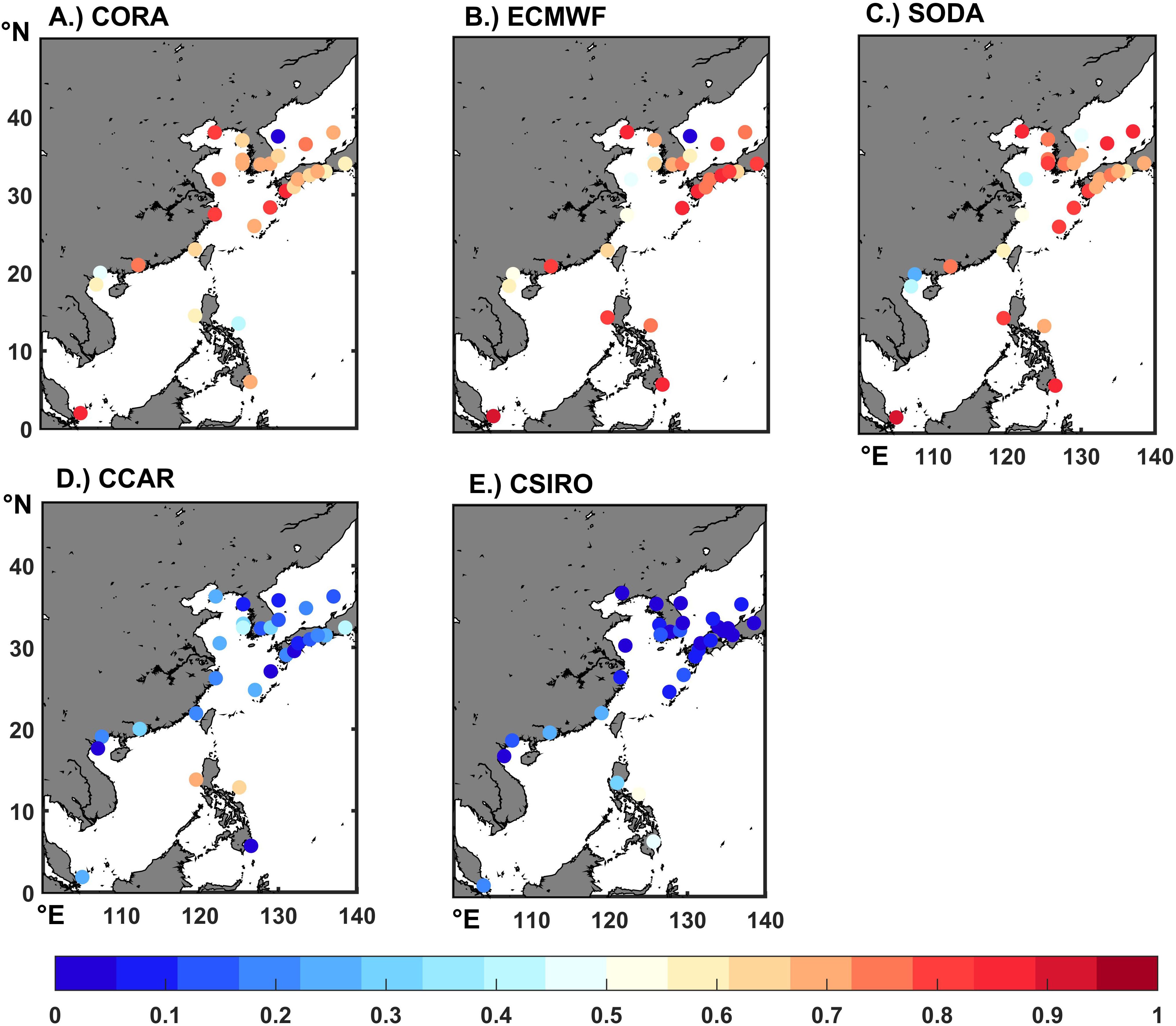
Figure 5. Correlation between tide gauges and products needing evaluation over the period 1960-2008. Each time series is subjected to a 5-year running mean and detrended before the correlation is computed (A–E: Different products).

We compared the reflections of tide gauges and products on the rate of sea level variations from 1960 to 2008 to investigate their consistency (Figure 6), in which the tide gauges were negative in nearly 10 stations in the Bohai Sea, Yellow Sea, and Sea of Japan, among which two stations, HONNGU and NAHA, were affected by the land subsidence and by the winds from the ground, resulting in an abnormal result of -5 mm/year. The ODAs datasets (Figures 6A, B, C) reflect the overall lower rate of sea level variation compared with the TGRs, in which the CORA and ECMWF are more detailed in portraying the spatial scale of sea level variations, and the CORA dataset portrays the rate of sea level variations in the near-shore shallow waters with a negative value of basically -2 mm/year, while the SODA dataset does not reflect the spatial variations of sea level as well. The TGRs (Figures 6D, E) reflected the sea level variability rate with positive values, the mean value is at 2.5 mm/year, among which the CCAR portrayed the spatial distribution of sea level in a more meticulous way, which can reflect the change of swirls in the mainstream region of the Kuroshio, and reached the maximum value of 3.5 mm/year in the Pacific Ocean.

Figure 6

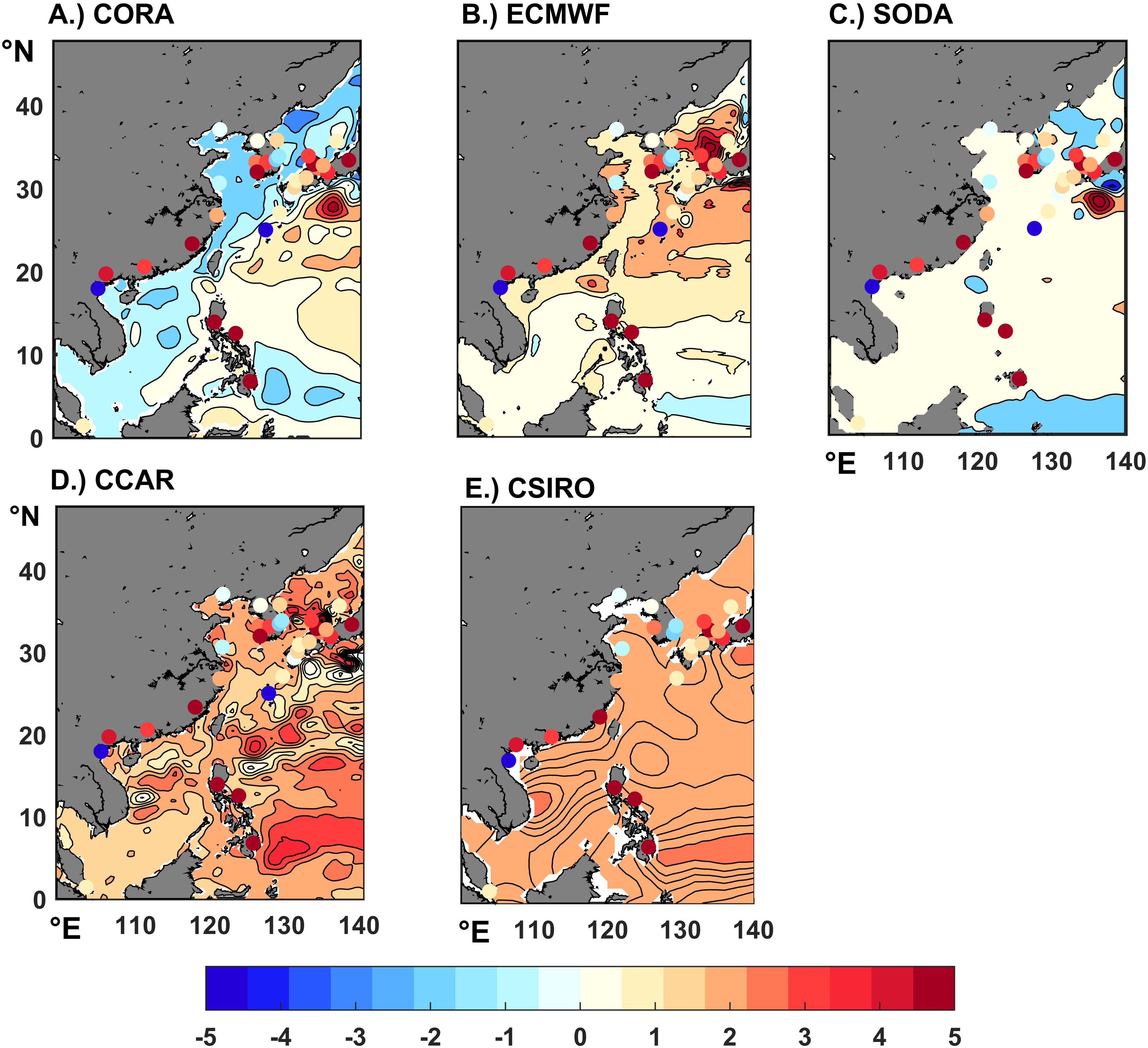
Figure 6. Trends measured by growth rate in tide gauges (colored dots) and each product (contour maps) over the period 1960-2008. (Unit: mm/year ; A–E: Different products).

All reconstructed datasets can describe the decadal cycle and rising trend of sea level variability satisfactorily, and each dataset has its differences in comparison with the data from the six representative stations. In the comparison between the reconstructed datasets and the tide gauge stations, the correlation between the TGRs datasets and the tide gauge stations is much lower than the ODAs, but each of them has its advantages and disadvantages in reflecting the rate of sea level variability, among which, CORA, CCAR, and ECMWF portray the spatial distribution of sea level variability better.

3.3 Compared to satellite altimetry data

We further computed the correlation between the satellite altimetry data (AVISO) and each reconstructed dataset during the satellite altimetry era (1993-2008) in Figure 7. Overall, the correlation between the ODAs (CORA, ECMWF, SODA), and AVISO is significantly stronger compared to TGRs (CCAR, CSIRO), especially in nearshore shallow areas and the Pacific. The CORA dataset (Figure 7A) shows the best correlation with AVISO in the China Sea as well as in the offshore range, and the correlation is greater than 0.8 in most of the regions except in the Sea of Japan region where the correlation is 0.3, which is the lowest value. In contrast, the correlation between ECMWF (Figure 7B) and SODA (Figure 7C), and AVISO in the Sea of Japan and the South China Sea is not very high, which is lower than 0.2. For the TGRs dataset, the correlation of the satellite altimetry data shows better in Southeast Luzon, while it is below 0.4 in all other regions (Figures 7D, E). The CSIRO dataset, however, shows worse performance, considering its lower spatial resolution (1 × 1 mth).

Figure 7

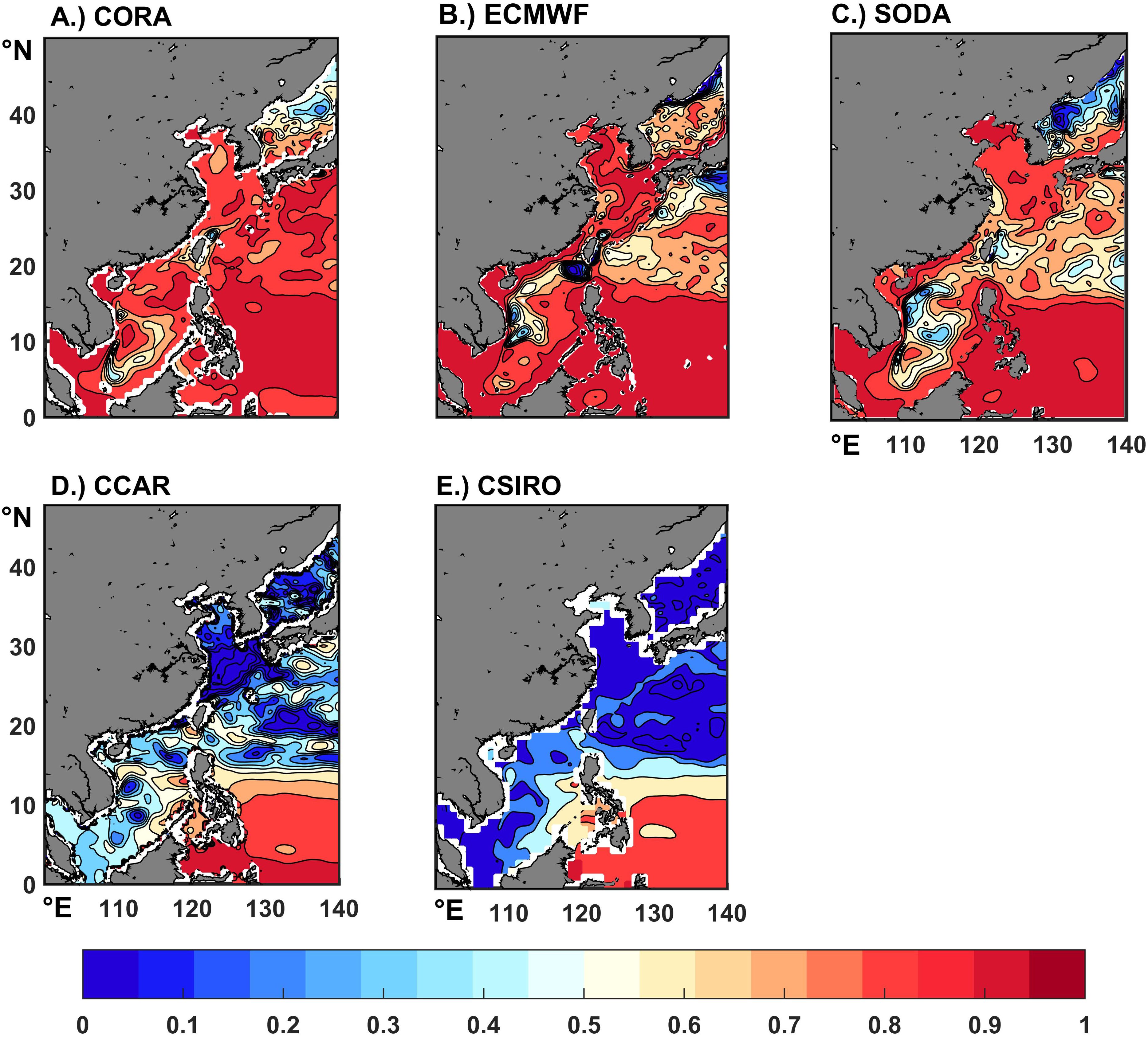
Figure 7. Correlation between the altimetry data (AVISO) and products needing evaluation over the period 1993-2008. The correlation is calculated after a 5-year running mean that has been applied to each time series, and all have been detrended (A–E: Different products).

We further compared the contrast between the rate of the satellite altimetry and each product dataset for the period 1993-2008 (Figure 8). It can be seen that the rate of AVISO is positive in the study area except for the central part of the Penghu Islands (Figure 8F). During the satellite altimetry era, the sea level rate of TGRs (CCAR and CSIRO) was closely aligned with AVISO, exhibiting modest increases in nearshore shallow areas and significant increases in the Pacific Ocean (approximately 7-10 mm/year). However, both TGRs and ODAs datasets underestimate the rate of sea level variability in the shelf seas, with CORA (Figure 8A) being negative in the Bohai Sea, parts of the East China Sea and the South China Sea, and the Sea of Japan, meaning that CORA significantly underestimates the sea level variability of the marginal seas on a 16-year cycle, while ECMWF and SODA (Figures 8B, C) perform slightly better than the former, and perform more consistently with AVISO in the Pacific Ocean, but also show negative values in the South China Sea or some parts of the Sea of Japan.

Figure 8

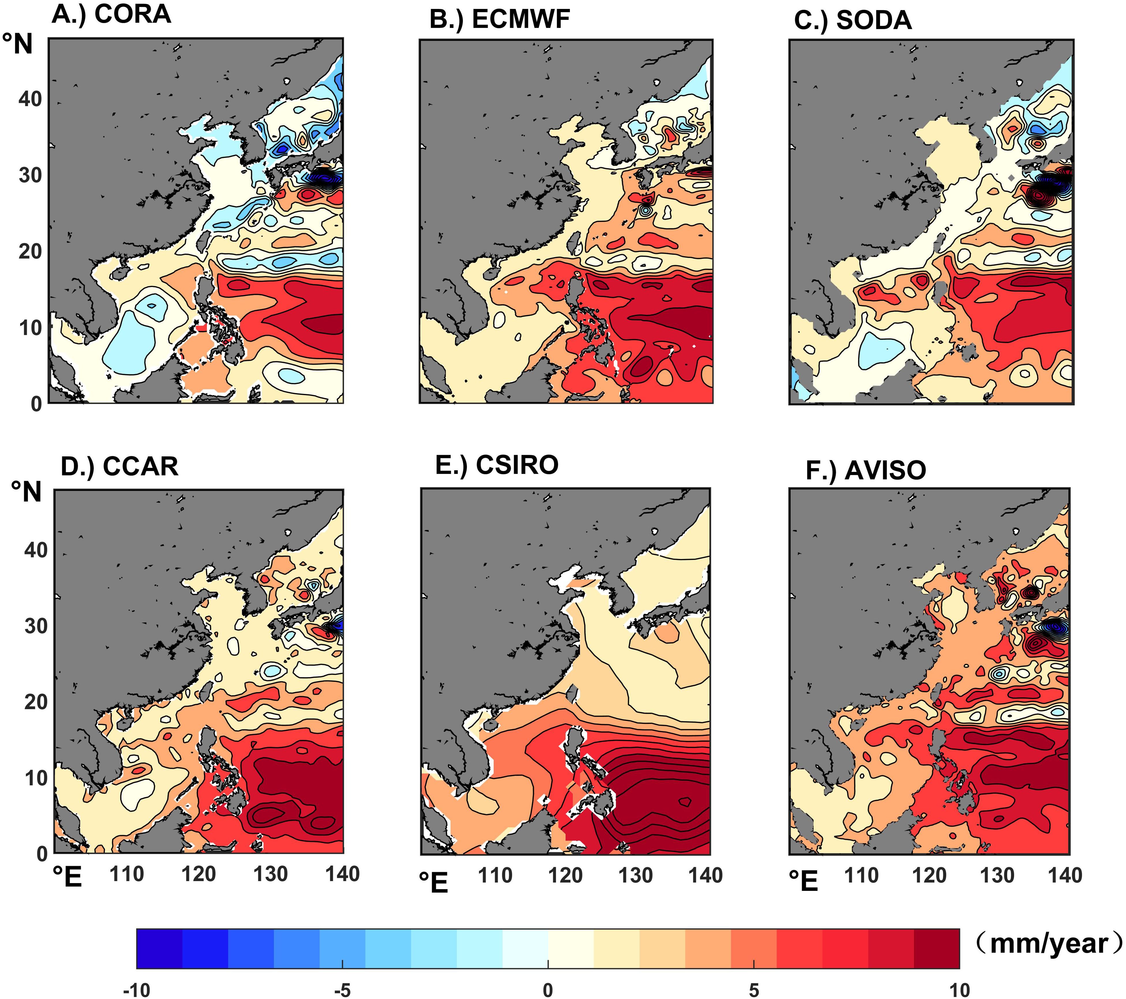
Figure 8. The trend measured by growth rate of sea level anomaly during the period from 1993 to 2008. (Unit: mm/year ; A–E: Different products; F: AVISO).

To assess the ability of each dataset to reproduce low-frequency variability, we calculated the standard deviation (Carson et al., 2017) over the period from 1960 to 2008, using the satellite altimetry data from 1993 to 2008 as a reference in Figure 9. In nearshore shallow waters such as the Sea of Japan, the Bohai Sea, the northern of the Yellow Sea, the eastern of the East China Sea, and the South China Sea, the variability of satellite altimetry sea level is around 10mm, while reaches its maximum variability in the Pacific Ocean east of the Philippines and along the southern coast of the island of Japan (refer to Figure 9F). TGRs (CCAR and CSIRO) also show maximum values in the Pacific region but perform poorly in capturing low-frequency variability in shallow nearshore waters and CSIRO, in particular, does not portray low-frequency variability well in spatial variation. The CCAR has higher variability in shallow nearshore waters, contradicting the characterization of altimetric sea level (Figure 9D). Correspondingly, the ODAs (CORA, SODA, ECMWF) exhibit a higher capability in capturing the low-frequency variability in nearshore areas, but it significantly underestimates the variability in the Pacific Ocean (Figures 9A–C). It’s noteworthy that, except CSIRO, all other products perform well along the coast of southern Japan Island. In conclusion, TGRs and ODAs have their strengths and weaknesses in making standard deviation reflections of low-frequency variability, with the former responding better to the oceanic region and the latter to the shelf-marginal sea region.

Figure 9

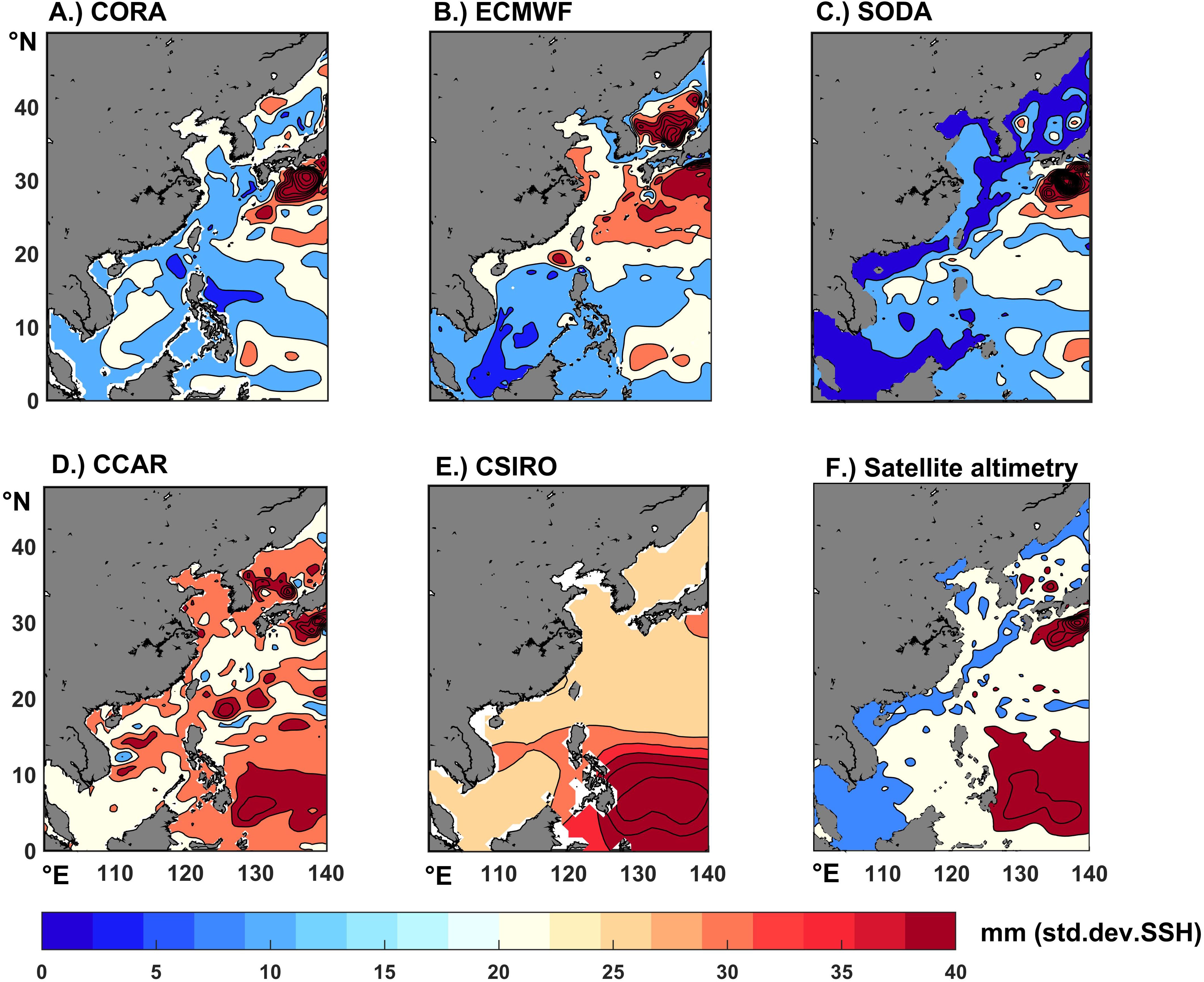
Figure 9. Interdecadal variability was calculated by applying a 5-year running mean with a Hanning window to the annual data and plotting the standard deviation. The data coverage is over the entire common period for the products, 1960-2008. (Unit: mm; A–E: Different products; F: Satellite altimetry).

As shown in Figure 10, to investigate the influences of PDO on regional sea level, we further calculated the correlation between each tide gauge station and the PDO index. It can be seen that all stations except HONNGU and DAVAO are in negative correlation, and nearly 75% of the tide gauge stations have a correlation between -0.1 and 0 with the PDO index (Figure 10F). The correlation between ECMWF (Figure 10B)/SODA (Figure 10C)/CSIRO (Figure 10E) with PDO is closer to the tide gauge stations, with over 95% of the correlations for tide gauge stations showing a negative correlation. CORA (Figure 10A) showed a positive correlation with PDO between 0 and 0.1 at 23% of the stations, overestimating the correlation of PDO compared to the tide gauge stations, while CCAR (Figure 10D) significantly underestimated the correlation between PDO and the tide gauges, especially at the Bohai/Yellow Sea and the tide gauges along the coasts of the Korean Peninsula and the Japanese islands. The correlation reaches about -0.5, which is a misclassification of the PDO impact. In summary, the correlation between CSIRO, ECMWF, and SODA with PDO is closer to the tide gauge stations.

Figure 10

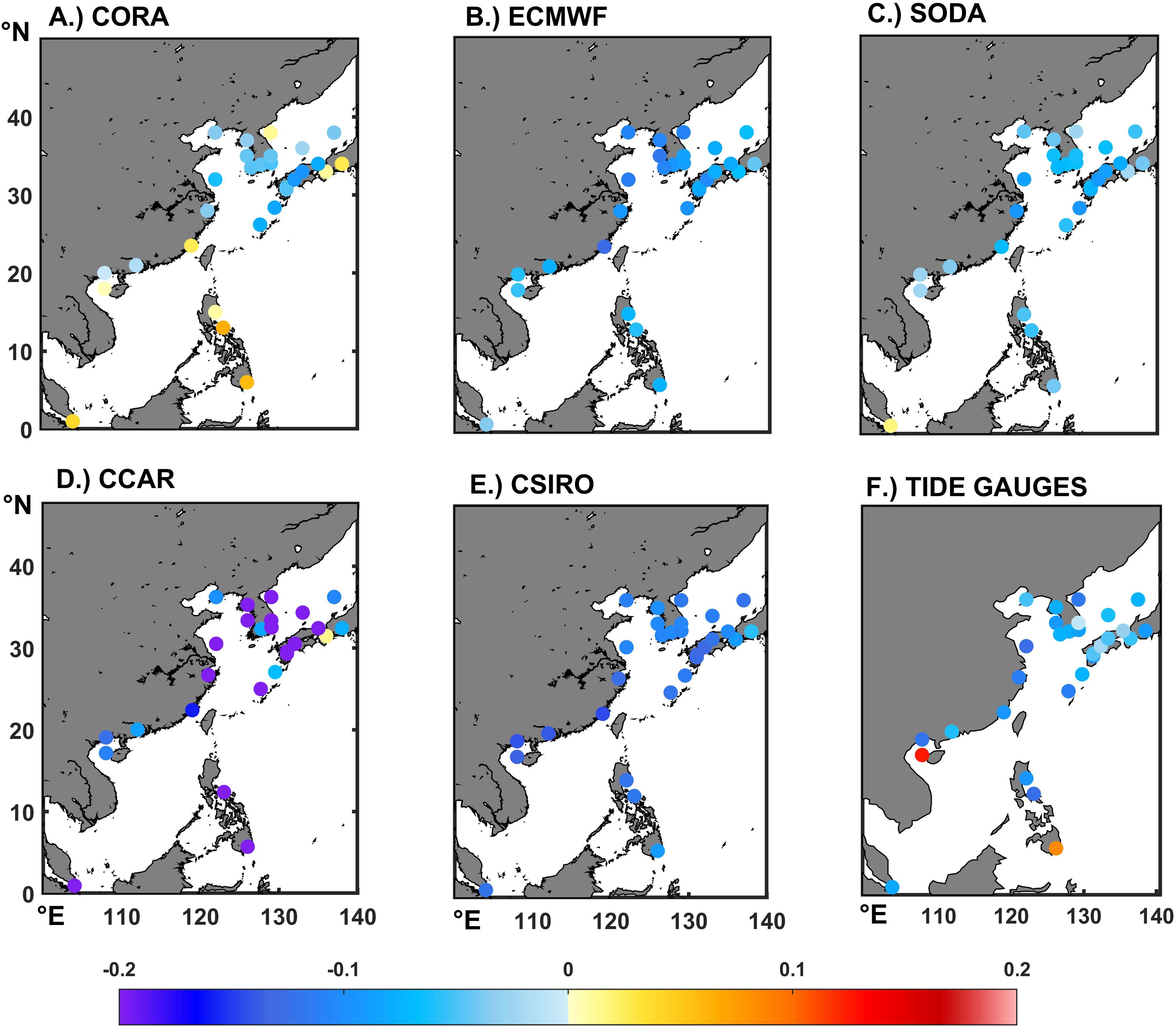
Figure 10. Correlation of the products including the tide gauges data with the PDO index over the period 1960-2008 to the influence of the Pacific Decadal Oscillation (PDO) on sea level (A–E: Different products; F: Tide gauges).

Comparison of each dataset with AVISO in the correlation, rate of sea level rise, and interannual interdecadal variability shows that the ODAs dataset has better correlation than the TGRs, but in terms of the response to the rate of sea level rise, while both have underestimation in some areas, the TGRs are better than the ODAs in a comprehensive sense, but the portrayal of sea level spatial variability by ODAs is also noteworthy. In the assessment of low-frequency variability of sea level, the TGRs dataset overestimates the impact of low-frequency variability, especially in the marginal sea area. All datasets perform obvious low correlation in capturing the PDO phenomenon.

4 Conclusion and discussion

In order to assess the reliability and accuracy of reconstructed sea level datasets in capturing the nuanced temporal patterns of sea level changes in the China Seas, a comprehensive analysis was conducted. Three ensembles of assimilated reconstructed data, labeled as ODA, along with two sets of reconstructed data obtained from tide gauge stations, referred to as TGR, were meticulously scrutinized. These datasets were rigorously compared against independent observations derived from both tide gauge stations and satellite altimetry measurements. The correlation and consistency of sea level time series, as well as the rate of sea level rise, and the inter-annual and inter-decadal variability inherent in the sea level signals across the selected datasets were evaluated.

Generally, positive correlations between ODAs and tide gauge stations in the China Sea and adjacent areas are observed, with correlations surpassing 0.6, except for a few anomalous stations. However, the correlation between CORA and ECMWF is slightly lower on both sides of the Korean Peninsula. Compared with the tide gauge data for the same period, the reflection of the rate of sea level variability in each dataset over the 1960-2008 time period shows that ODAs underestimate the sea level variability, with CORA/SODA being the most obvious, especially in the near-shore shallow waters. These differences may be due to the differences in the data assimilated, among which 3D-Var ocean data assimilation is used in CORA (Li et al., 2006; Xie et al., 2011), 4D-Var data assimilation is used in ECMWF. In addition, the POMgcs model used by CORA and the 3D-Var assimilated reconstructed data better preserve the sea level characteristics of the Chinese coastal areas and optimize the overfitting with the satellite altimetry data.

TGRs exhibit poor correlation with tide gauge stations in the China Sea and nearby regions. While, the TGRs provide a better reflection of sea level variability than the former over nearly 50 years, with CCAR providing the finest description of sea level variability in China and neighboring seas, while SODA and CSIRO provide less detailed descriptions of spatial variability in sea level. One factor contributing to this is the relatively smaller number of tide gauges around the China Seas compared to regions like North America and Europe, which are extensively utilized in TGRs (Parker, 2016). Additionally, the offshore region of China lies on the periphery of the continental shelf, characterized by distinct oceanic processes and structures compared to open ocean environments. Furthermore, TGR reconstruction products are influenced by corrections for local vertical land motion due to glacial isostatic adjustment (GIA), tectonic shifts, and other perturbing factors encountered during measurement, as highlighted in prior studies (Church et al., 2004; Peltier, 2004; Carson et al., 2017). Consequently, the local environment plays a significant role, contributing to the observed poor correlation.

In terms of correlation with satellite altimetry datasets, ODAs exhibit superior correlation compared to TGRs, with CORA displaying notably higher correlation, particularly in the coastal waters of China and the Pacific region, where correlations reach 0.8 and above. However, ODAs demonstrate inconsistency with altimetry datasets in reflecting the rate of sea level rise, but all have underestimated sea level variability over the 1993-2008 time period, especially in shallow marginal waters such as the Bohai Sea. This disparity varies among assimilated products, likely due to a continuous positive acceleration influencing the time-series increase trend during the reconstruction process, leading to overfitting satellite altimetry data through multiple alignments to the most recent (Parker, 2016). The CORA dataset exhibits satisfactory performance in several aspects, except for accurately reflecting the rate of sea level rise, which tends to be consistently underestimated. TGRs reflect sea level variability better than ODAs, but the CSIRO portrayal of sea level on spatial scales is less detailed over these 15a. Consistent with the performance of CSIRO on a global scale.

In terms of reflecting low-frequency variability over 15a compared to altimetry data, the TGRs exhibit an overestimation in the vicinity of China and adjacent seas. Conversely, the ODAs, while displaying greater similarity to each other in terms of low-frequency variability, generally manifest weaker signals compared to TGRs. This finding aligns with global-scale results. Carson et al. (2017) postulated that these disparities between ODAs and TGRs may stem from the inadequate resolution inherent in earlier, truncated altimetry records, which fail to capture the nuanced lower-frequency variability prevalent in the region. Furthermore, the operational disparities between tide gauges in shelf seas and those in open oceanic settings accentuate the need for bespoke methodologies to accurately depict their respective variations.

Regarding correlation with the PDO, the reconstructed products demonstrate consistent low correlation, with ODAs lightly closer with tide gauges than TGRs. This superiority of ODAs is attributed partly to the limited coverage of tide gauge stations by TGRs, particularly along the Asian coast, resulting in fewer valid data points. Consequently, the statistical reconstruction derived from tide gauge data inadequately represents shallow coastal areas. In contrast, assimilated datasets exhibit robust consistency with altimetry data, effectively capturing inter-decadal sea level variability along the coast of China and its adjacent marginal seas.

It is noteworthy that the current portrayals of regional sea level variability preceding the satellite era are constrained and lack robust conclusions regarding their patterns and variability. Our analysis indicates that Ocean Data Assimilations (ODAs) and Tide Gauge Reconstructions (TGRs) exhibit differing strengths and weaknesses in capturing sea level variability. The findings of our study have important implications for coastal management and climate adaptation strategies. Also, our results suggests the need for further research to refine existing reconstruction methodologies. Future studies could investigate hybrid approaches that integrate the strengths of both ODAs and TGRs to enhance overall accuracy in sea level projections, particularly in regions with limited tide gauge coverage. Also, the findings underscore the potential of incorporating additional variables such as sea surface temperature, wind patterns, and atmospheric pressure into the reconstruction process (Chen et al., 2017). At last, given the discrepancies observed due to limited tide gauge coverage, there is a clear need for enhanced long-term monitoring of sea levels, particularly in the China Seas and neighboring regions. Future efforts should focus on expanding the network of tide gauge stations and employing advanced remote sensing technologies to fill data gaps.

Data availability statement

The original contributions presented in the study are included in the article/supplementary material. Further inquiries can be directed to the corresponding author.

Author contributions

SZ: Data curation, Investigation, Software, Writing – original draft. YL: Formal analysis, Validation, Writing – original draft, Methodology. JF: Formal analysis, Methodology, Supervision, Writing – review & editing. YJ: Data curation, Formal analysis, Visualization, Writing – review & editing. JZ: Project administration, Resources, Validation, Writing – review & editing. LZ: Project administration, Resources, Supervision, Validation, Writing – review & editing.

Funding

The author(s) declare financial support was received for the research, authorship, and/or publication of this article. This work is supported by The National Natural Science Foundation of China (No. 42176198). Supported by The Key Laboratory of Ocean Observation and Information of Hainan Province (Open Fund Project No. HKLOOI-OF-2023-03).

Conflict of interest

The authors declare that the research was conducted in the absence of any commercial or financial relationships that could be construed as a potential conflict of interest.

Publisher’s note

All claims expressed in this article are solely those of the authors and do not necessarily represent those of their affiliated organizations, or those of the publisher, the editors and the reviewers. Any product that may be evaluated in this article, or claim that may be made by its manufacturer, is not guaranteed or endorsed by the publisher.

References

Adebisi N., Balogun A. L., Min T. H., Tella A. (2021). Advances in estimating sea level rise: A review of tide gauge, satellite altimetry and spatial data science approaches. Ocean Coast. Manage. 208, 105632. doi: 10.1016/j.ocecoaman.2021.105632

Crossref Full Text | Google Scholar

Barnston A. G., van den Dool H. M. (1993). Toward understanding the causes of low-frequency variability: the interannual standard deviation of monthly mean 700-mb height. J. Climate. 6, 2083–2102. doi: 10.1175/1520-0442(1993)006<2083:TUTCOL>2.0.CO;2

Crossref Full Text | Google Scholar

Beckley B. D., Lemoine F. G., Luthcke S. B., Ray R. D., Zelensky N. P. (2007). A reassessment of global and regional mean sea level trends from TOPEX and Jason-1 altimetry based on revised reference frame and orbits. Geophys. Res. Lett. 34, L14608. doi: 10.1029/2007GL030002

Crossref Full Text | Google Scholar

Bing C., Qiang Z. (2018). GIA model statistics for GRACE hydrology, cryosphere, and ocean science. Geophys. Res. Letters. 45, 2203–2212. doi: 10.1002/2017gl076644

Crossref Full Text | Google Scholar

Carson M., Köhl A., Stammer D., Meyssignac B., Church J., Schröter J., et al. (2017). Regional sea level variability and trends 1960–2007: A comparison of sea level reconstructions and ocean syntheses. J. Geophys. Res. Ocean. 122, 9068–9091. doi: 10.1002/2017jc012992

Crossref Full Text | Google Scholar

Carton J. A., Giese B. S. (2008). A reanalysis of ocean climate using simple ocean data assimilation (SODA). Mon Weather Rev. 136, 2999–3017. doi: 10.1175/2007MWR1978.1

Crossref Full Text | Google Scholar

Chambers D. P., Mehlhaff C. A., Urban T. J., Fujii D., Nerem R. S. (2002). Low-frequency variations in global mean sea level: 1950–2000. J. Geophys. Res. Ocean 107, 1–1-1-10. doi: 10.1029/2001JC001089

Crossref Full Text | Google Scholar

Chen X., Zhang X., Church J. A., Watson C. S., King M. A., Monselesan D., et al. (2017). The increasing rate of global mean sea-level rise during 1993–2014. Nat. Clim Change. 7, 492–495. doi: 10.1038/nclimate3325

Crossref Full Text | Google Scholar

Cheng Y. C., Ezer T., Hamlington B. D. (2016). Sea level acceleration in the China Seas. Water 8 (7), 293. doi: 10.3390/w8070293

Crossref Full Text | Google Scholar

Cheng Y., Hans P. P., Hamlington B. D., Xu Q., He Y. J. (2015). Regional sea level variability in the Bohai Sea, Yellow Sea, and East China Sea. Cont Shelf Res. 111, 95–107. doi: 10.1016/j.csr.2015.11.005

Crossref Full Text | Google Scholar

Church J., Gregory J., White N., Platten S., Mitrovica J. (2011). Understanding and projecting sea level change. Oceanography 24, 130–143. doi: 10.5670/oceanog.2011.33

Crossref Full Text | Google Scholar

Church J. A., White N. J. (2006). A 20th century acceleration in global sea-level rise. Geophys. Res. Lett. 33, L01602. doi: 10.1029/2005GL024826

Crossref Full Text | Google Scholar

Church J. A., White N. J., Coleman R., Lambeck K., Mitrovica J. X. (2004). Estimates of the regional distribution of sea level rise over the 1950–2000 period. J. Clim. 17, 2609–2625. doi: 10.1175/1520-0442(2004)017<2609:EOTRDO>2.0.CO;2

Crossref Full Text | Google Scholar

Cipollini P., Calafat F. M., Jevrejeva S., Melet A., Prandi P. (2017). Monitoring sea level in the coastal zone with satellite altimetry and tide gauges. Surv Geophys. 38, 33–57. doi: 10.1007/s10712-016-9392-0

PubMed Abstract | Crossref Full Text | Google Scholar

Dubrovský M., Buchtele J., Žalud Z. (2004). High-frequency and low-frequency variability in stochastic daily weather generator and its effect on agricultural and hydrologic modelling. Climatic Change. 63, 145–179. doi: 10.1023/b:Clim.0000018504.99914.60

Crossref Full Text | Google Scholar

Fang J., Wahl T., Zhang Q., Muis S., Hu P., Fang J., et al. (2021). Extreme sea levels along coastal China: uncertainties and implications. Stoch Env. Res. Risk A. 35, 405–418. doi: 10.1007/s00477-020-01964-0

Crossref Full Text | Google Scholar

Feng J., Li D., Li Y., Zhao L. (2023). Analysis of compound floods from storm surge and extreme precipitation in China. J. Hydrol. 627, 130402. doi: 10.1016/j.jhydrol.2023.130402

Crossref Full Text | Google Scholar

Feng X., Tsimplis M. N., Marcos M., Calafat F. M., Zheng J., Jordà G., et al. (2015). Spatial and temporal variations of the seasonal sea level cycle in the northwest Pacific. J. Geophys. Res. Ocean. 120, 7091–7112. doi: 10.1002/2015JC011154

Crossref Full Text | Google Scholar

Giese B. S., Ray S. (2011). El Niño variability in simple ocean data assimilation (SODA), 1871–2008. J. Geophys. Res. Ocean. 116, C02024. doi: 10.1029/2010JC006695

Crossref Full Text | Google Scholar

Guérou A., Meyssignac B., Meyssignac B., Prandi P., Ablain M., Ribes A., et al. (2023). Current observed global mean sea level rise and acceleration estimated from satellite altimetry and the associated measurement uncertainty. Ocean Sci. 19, 431–451. doi: 10.5194/os-19-431-2023

Crossref Full Text | Google Scholar

Guo J., Hu Z., Wang J., Chang X., Li G. (2015). Sea level changes of China seas and neighboring ocean based on satellite altimetry missions from 1993 to 2012. J. Coast. Res. 31, 17–21. doi: 10.2112/si73-004.1

Crossref Full Text | Google Scholar

Hallegatte S., Green C., Nicholls R. J., Corfee-Morlot J. (2013). Future flood losses in major coastal cities. Nat. Clim Change 3, 802–806. doi: 10.1038/nclimate1979

Crossref Full Text | Google Scholar

Hamlington B. D., Burgos A., Thompson P. R., Landerer F. W., Piecuch C. G., Adhikari S., et al. (2018). Observation driven estimation of the spatial variability of 20th century sea level rise. J. Geophys. Res. Ocean. 123, 2129–2140. doi: 10.1002/2017JC013486

Crossref Full Text | Google Scholar

Hamlington B. D., Cheon S. H., Piecuch C. G., Karnauskas K. B., Thompson P. R., Kim K.-Y., et al. (2019). The dominant global modes of recent internal sea level variability. J. Geophys. Res. Ocean. 124, 2750–2768. doi: 10.1029/2018JC014635

Crossref Full Text | Google Scholar

Hamlington B. D., Cheon S. H., Thompson P. R., Merrifield M. A., Nerem R. S., Leben R. R., et al. (2016). An ongoing shift in Pacific Ocean sea level. J. Geophys. Res. Ocean. 121, 5084–5097. doi: 10.1002/2016JC011815

Crossref Full Text | Google Scholar

Hamlington B. D., Leben R. R., Kim K.-Y. (2012a). Improving sea level reconstructions using non-sea level measurements. J. Geophys. Res. Ocean 117, C10025. doi: 10.1029/2012JC008277

Crossref Full Text | Google Scholar

Hamlington B. D., Leben R. R., Nerem R. S., Han W., Kim K. Y. (2011). Reconstructing sea level using cyclostationary empirical orthogonal functions. J. Geophys. Res. Ocean 116, C12015. doi: 10.1029/2011JC007529

Crossref Full Text | Google Scholar

Hamlington B. D., Leben R. R., Wright L. A., Kim K. Y. (2012b). Regional sea level reconstruction in the Pacific Ocean. Mar. Geod. 35, 98–117. doi: 10.1080/01490419.2012.718210

Crossref Full Text | Google Scholar

Han G., Fu H., Zhang X., Li W., Wu X., Wang X., et al. (2013a). A global ocean reanalysis product in the China Ocean Reanalysis (CORA) project. Adv. Atmos. Sci. 30, 1621–1631. doi: 10.1007/s00376-013-2198-9

Crossref Full Text | Google Scholar

Han G., Li W., Zhang X., Li D., He Z., Wang X., et al. (2011). A regional ocean reanalysis system for coastal waters of China and adjacent seas. Adv. Atmos. Sci. 28, 682–690. doi: 10.1007/s00376-010-9184-2

Crossref Full Text | Google Scholar

Han G., Li W., Zhang X., Wang X., Wu X., Fu H., et al. (2013b). A new version of regional ocean reanalysis for coastal waters of China and adjacent seas. Adv. Atmos. Sci. 30, 974–982. doi: 10.1007/s00376-012-2195-4

Crossref Full Text | Google Scholar

Han W., Meehl G. A., Stammer D., Hu A., Hamlington B., Kenigson J., et al. (2017). Spatial patterns of sea level variability associated with natural internal climate modes. Surv Geophys. 38, 217–250. doi: 10.1007/s10712-016-9386-y

PubMed Abstract | Crossref Full Text | Google Scholar

Hay C. C., Morrow E., Kopp R. E., Mitrovica J. X. (2015). Probabilistic reanalysis of twentieth-century sea-level rise. Nature 517, 481–484. doi: 10.1038/nature14093

PubMed Abstract | Crossref Full Text | Google Scholar

Horton B. P., Khan N. S., Cahill N., Lee J. S. H., Shaw T. A., Garner A. J., et al. (2020). Estimating global mean sea-level rise and its uncertainties by 2100 and 2300 from an expert survey. NPJ Clim. Atmos. Sci. 3, 1–8. doi: 10.1038/s41612-020-0126-0

Crossref Full Text | Google Scholar

Kumar P., Hamlington B., Cheon S. H., Han W., Thompson P. (2020). 20th century multivariate Indian Ocean regional sea level reconstruction. J. Geophys. Res. Ocean. 125, e2020JC016270. doi: 10.1029/2020JC016270

Crossref Full Text | Google Scholar

Leuliette E. W., Nerem R. S., Mitchum G. T. (2004). Calibration of TOPEX/Poseidon and Jason altimeter data to construct a continuous record of mean sea level change. Mar. Geod. 27, 79–94. doi: 10.1080/01490410490465193

Crossref Full Text | Google Scholar

Li W., Xie Y., He Z., Han G., Liu K., Ma J., et al. (2006). Application of the multigrid data assimilation scheme to the China Seas’ temperature forecast. J. Atmos. Ocean Tech. 25, 2106–2116. doi: 10.1175/2008JTECHO510.1

Crossref Full Text | Google Scholar

Liu H., Cheng X., Qin J., Zhou G., Jiang L. (2023). The dynamic mechanism of sea level variations in the Bohai Sea and Yellow Sea. Clim Dynam. 61, 2937–2947. doi: 10.1007/s00382-023-06724-8

Crossref Full Text | Google Scholar

Liu C., Li X., Wang S., Tang D., Zhu D. (2020). Interannual variability and trends in sea surface temperature, sea surface wind, and sea level anomaly in the South China Sea. Int. J. Remote Sens. 41, 4160–4173. doi: 10.3390/atmos12040454

Crossref Full Text | Google Scholar

Manabe S., Stouffer R. J. (1996). Low-frequency variability of surface air temperature in a 1000-year integration of a coupled atmosphere-ocean-land surface model. J. Climate. 9, 376–393. doi: 10.1175/1520-0442(1996)0092.0.CO;2

Crossref Full Text | Google Scholar

Milne G. A., Gehrels W. R., Hughes C. W., Tamisiea M. E. (2009). Identifying the causes of sea-level change. Nat. Geosci. 2, 471–478. doi: 10.1038/ngeo544

Crossref Full Text | Google Scholar

Mu D., Xu T., Yan H. (2024). Sea level rise along China coast from 1950 to 2020. Sci. China Earth Sci. 67, 802–810. doi: 10.1007/s11430-023-1240-x

Crossref Full Text | Google Scholar

Nerem R. S., Chambers B. D., Hamlington R. R., Leben G., Mitchum T., Phillips T., Willis I. K. (2010). Observations of recentsea level change, paper presented at the IPCC Workshop on Sea Level Rise and lce Sheet Instabilities, Intergov. Panel on Clim. Change, Malaysia, June.

Google Scholar

Parker A. (2016). The actual measurements at the tide gauges do not support strongly accelerating twentieth-century sea-level rise reconstructions. Nonlinear Eng. 5, 45–71. doi: 10.1515/nleng-2015-0006

Crossref Full Text | Google Scholar

Peltier W. R. (2004). Global glacial isostasy and the surface of the ice-age Earth: the ICE-5G (VM2) model and GRACE. Annu. Rev. Earth Pl Sc. 32, 111–149. doi: 10.1146/annurev.earth.32.082503.144359

Crossref Full Text | Google Scholar

Ray R. D., Douglas B. C. (2011). Experiments in reconstructing twentieth-century sea levels. Prog. Oceanogr. 91, 496–515. doi: 10.1016/j.pocean.2011.07.021

Crossref Full Text | Google Scholar

Sheng F. (2016). The sea level change and projection along the coast of China under the background of global warming. [master’s thesis]. [Nanjing(Jiang Su)]: Nanjing University of Information Science and Technology.

Google Scholar

Smith R. D., Dukowicz J. K., Malone R. C. (1992). Parallel ocean general circulation modeling. Phys. D: Nonlinear Phenom. 60, 38–61. doi: 10.1016/0167-2789(92)90225-c

Crossref Full Text | Google Scholar

Strassburg M. W., Hamlington B. D., Leben R. R., Manurung P., Lumban Gaol J., Nababan B., et al. (2015). Sea level trends in Southeast Asian seas. Clim. Past. 11, 743–750. doi: 10.5194/cp-11-743-2015

Crossref Full Text | Google Scholar

Xie Y., Koch S., McGinley J., Albers S., Bieringer P. E., Wolfson M., et al. (2011). A space–time multiscale analysis system: a sequential variational analysis approach. Mon Weather Rev. 139, 1224–1240. doi: 10.1175/2010MWR3338.1

Crossref Full Text | Google Scholar

Zhou D., Liu Y., Feng Y., Zhang H., Fu Y., Liu Y., et al. (2022). Absolute sea level changes along the coast of China from tide gauges, GNSS, and satellite altimetry. J. Geophys. Res. Ocean. 127, e2022JC018994. doi: 10.1029/2022JC018994

Crossref Full Text | Google Scholar

Zuo H., Balmaseda M., Tietsche S., Mogensen K., Mayer M. (2019). The ECMWF operational ensemble reanalysis–analysis system for ocean and sea ice: a description of the system and assessment. Ocean Sci. 15, 779–808. doi: 10.5194/os-15-779-2019

Crossref Full Text | Google Scholar