Robust sensor selection based on maximum correntropy criterion for ocean data reconstruction

Selecting an optimal subset of sensors that can accurately reconstruct the full state of the ocean can reduce the cost of the monitoring system and improve monitoring efficiency. Typically, in data-driven sensor selection processes, the use of Euclidean distance to evaluate reconstruction error is susceptible to non-Gaussian noise and outliers present in ocean data. This paper proposes a Robust Sensor Selection (RSS) evaluation model based on the Maximum Correntropy Criterion (MCC) through subspace learning, enabling the selection of robust sensor measurement subsets and comprehensive data reconstruction. To more accurately quantify the impact of varying noise magnitudes, noise weights were incorporated into the model’s objective function. Additionally, the local geometric structure of data samples is utilized to further enhance reconstruction accuracy through the selected sensors. Subsequently, the MCC_RSS algorithm is proposed, which employs the Block Coordinate Update (BCU) method to achieve the optimal solution for the proposed model. Experiments conducted using ocean temperature and salinity datasets validate the proposed MCC_RSS algorithm. The results demonstrate that the sensor selection method proposed in this paper exhibits strong robustness, outperforming comparative methods under varying proportions of outliers and non-Gaussian noise.

1 Introduction

In the field of oceanography, optimizing sensor selection is a critical area of research. Effective sensor selection can directly impact sensor deployment and enhance our understanding of the oceanic physical parameters. By tailoring sensor selection to meet specific requirements, various objectives can be achieved, including cost reduction (Emily et al., 2020; Saito et al., 2023), energy efficiency (Ghosh et al., 2021), conservation of communication resource (Yang et al., 2015), assistance in localization (Mei et al., 2024), improved field reconstructions (Santini and Colesanti, 2009; Zhang et al., 2018; Nguyen et al., 2021; Santos et al., 2023) and enhanced state predictions (Saucan and Win, 2020; Patan et al., 2022), among others.

The sensor selection problem involves selecting the optimal p positions from n candidate positions to achieve the desired outcomes, a task recognized as NP-hard (Chamon et al., 2021). This implies that an exhaustive search would need to traverse up to $n!/[p!(n-p)!]$ combinations, which is nearly impossible when the number of candidate positions is large in ocean monitoring. General solutions to the sensor selection problem include the following: convex optimization (Joshi and Boyd, 2009), statistical methods (Chepuri and Leus, 2015; Lin et al., 2019; Yamada et al., 2021), heuristic methods (Khokhlov et al., 2019; Zhao et al., 2021; Meray et al., 2023), information theory (Krause et al., 2008; Prakash and Bhushan, 2023), dimensionality reduction (Yildirim et al., 2009; Manohar et al., 2018; Jayaraman et al., 2019), machine learning-based clustering (Kalinić et al., 2022), among others.

Data-driven sensor selection provides an excellent optimization solution for selecting sensors from a large pool of candidate locations in ocean monitoring. By analyzing the intrinsic characteristics of known data, it identifies the most critical geographical locations for reconstructing the entire physical field, without requiring precise modeling or complex statistical analysis of the monitoring object or requirements. However, these methods typically evaluate the reconstruction effect based on the Euclidean distance between the original and reconstructed data, which is highly sensitive to non-Gaussian noise and outliers. This sensitivity is particularly problematic in ocean monitoring, where specific sudden events (such as tsunamis causing sensor failure, communication interruptions, or data loss) can significantly impact data quality. Consequently, noise in the data can severely affect the effectiveness of sensor deployment. Moreover, greedy algorithms such as Proper Orthogonal Decomposition (POD) and QR decomposition cannot guarantee globally optimal results.

Building on the work of Zhou et al. (2019) on Maximum Correntropy Criterion-based sparse subspace learning for feature selection, we propose a novel sparse sensor selection method. This method quantifies the similarity between the original data and the reconstructed data using correntropy, thereby effectively mitigating the impact of outliers on the feature selection process. Additionally, the subspace learning approach allows for the simultaneous updating of the feature selection matrix and the reconstruction matrix, enhancing the accuracy of the reconstruction.

This work employs subspace learning based on the Maximum Correntropy Criterion (MCC) for sensor selection. The main contributions of this study are as follows:

● The application of the MCC for evaluating reconstruction error supersedes the traditional Euclidean distance, thereby enhancing the stability of results in the presence of non-Gaussian noise and outliers. Additionally, noise weight is employed to measure the MCC, and the higher entropy of noise weight is utilized to achieve a noise distribution that more accurately represents the distribution of real system variables.

● In order to further improve reconstruction accuracy, a term that preserves the local geometric structure between samples was incorporated into the objective function to minimize the similarity between the selected measurements.

● The adoption of subspace learning allows for the simultaneous determination of both the sensor selection matrix and the mapping for data reconstruction from low-dimensional measurements to high-dimensional measurements corresponding to this selection matrix.

● Experiments conducted on ocean temperature and salinity datasets demonstrate that the proposed sparse sensor selection method exhibits robust performance.

Subsequently, we review the related work in Section 2. Section 3 introduces the sparse sensor deployment model based on MCC, with the solution algorithm detailed in Section 4. The proposed algorithm is validated using ocean temperature and salinity datasets in Section 5. Finally, Section 6 provides a summary and discussion.

2 Related works

The Euclidean distance is frequently utilized as a criterion for measuring the reconstruction error in sensor selection problems. Specifically, this involves using the Frobenius norm of the difference between the original data and the reconstructed data, as follows:

$\begin{array}{ll}C=\underset{C}{\arg \min }{\Vert X-\widehat{X}\Vert }_F& (1)\end{array}$

where $X\in {ℝ}^{n\times m}$ represents the original data, $\widehat{X}\in {ℝ}^{n\times m}$ represents the reconstructed data, $C\in {ℝ}^{p\times n}$ represents sensor selection matrix, n represents the number of all candidate locations for sensor selection, m represents the number of samples and p represents the number of sensors to be selected. Typically, once the sensor selection matrix C is established, the sensor’s measurement data can be acquired, which can be expressed as: $Y=CX$. By designing an appropriate mapping based on the measurement data Y, the reconstruction data $\widehat{X}$ can be obtained.

There is extensive research on data reconstruction aimed at determining the mapping from measurement data to original data. Examples include fluid reconstruction based on sparse representation (Callaham et al., 2019; Xue et al., 2019) and autoencoder networks (Erichson et al., 2020; Sahba et al., 2022). In these studies, the subset of locations is typically selected in a random manner. Some research focuses on mapping the original fluid data to low-dimensional features using deep neural networks (Özbay and Laizet, 2022; Zhang et al., 2023). These features reside in a subspace of the high-dimensional space and are not directly related to the sensor positions. Other research employs sensor selection by designing sensor positions according to specific partition rules, such as Voronoi tessellation (Fukami et al., 2021) or predetermined positions in a divided grid (Model and Zibulevsky, 2006), among others.

Algorithms for sensor selection and dimension reduction, such as the POD (Jayaraman et al., 2019) and QR decomposition (Manohar et al., 2018; Zhang et al., 2023), primarily map high-dimensional matrices to low-dimensional subspaces to obtain low-dimensional location indices. However, POD relies on a base matrix derived from Singular Value Decomposition (SVD) for data reconstruction, with sensors typically selected at random. In contrast, QR decomposition generally employs a greedy approach to identify low-dimensional location indices with the highest energy (e.g., spectral norm) to determine the measurement subset that can best reconstruct the original data. While a greedy approach focuses on the benefit of each individual step in the solution process, it often neglects the impact on the overall solution.

There are also sensor selection methods for reconstruction that integrate both dimension reduction and data reconstruction, such as data-driven sparse sensing (Jayaraman and Mamun, 2020), clustering for sensor select and regressive reconstruction in (Dubois et al., 2022) and compress sensing (Carmi and Gurfil, 2013; Joneidi et al., 2020). According to the research by Peherstorfer et al (Peherstorfer et al., 2020), the presence of noise in the data exacerbates the impact of the noise on the results as the number of selected locations increases. Furthermore, since these methods utilize Euclidean distance for similarity measurement, they are particularly susceptible to non-Gaussian noise or outliers in real-world marine monitoring scenarios.

To minimize the impact of noise, (Zhou et al. (2019) proposed a sparse subspace learning method based on MCC, which simultaneously searches for the feature selection matrix and the mapping. However, this method is primarily used for feature selection in image and sound data. Generally, MCC, grounded in the concept of correntropy from information theory, is adept at capturing nonlinear relationships and complex structures within data. This endows MCC with a significant advantage in handling complex datasets, enabling it to more accurately reflect the true characteristics of the data. By maximizing correntropy, MCC can effectively mitigate the influence of outliers on the model. Additionally, MCC does not depend on the specific distribution form of noise, thereby exhibiting excellent performance when dealing with non-Gaussian noise. Conversely, Guo et al. (Guo and Lin (2018) minimize the impact of noise by identifying the noise indicator of the maximum entropy distribution during low-rank matrix decomposition. These studies suggest that MCC and entropy-based noise indicators can provide a feasible solution for the problem of robust sparse sensor selection.

3 Model of robust sensor selection based on MCC

This section introduces a model for robust sensor selection. Initially, an error measure based on the Maximum Correntropy Criterion (MCC) is proposed to enhance the robustness of sensor selection. Subsequently, an objective function for the robust sensor selection model is formulated utilizing this error measure. To further augment the robustness of the model, noise indicators are established, which impose additional constraints on the objective function through the noise matrix.

3.1 Reconstruction error based on MCC

In Information Theoretic Learning (ITL), correntropy has proven effective in mitigating the impact of non-Gaussian noise and outliers (Liu et al., 2007). The MCC has demonstrated its efficacy in robust compressive sensing reconstruction (He et al., 2019). Consequently, within this context, MCC is utilized as a standard to evaluate the similarity between the original data and the reconstructed data for robust sensor selection, as follows:

For any two random variables A and B, the correntropy is defined as:

$\begin{array}{ll}V(A,B)=E[\kappa (A,B)]& (2)\end{array}$

where $E[\cdot ]$ represents the expectation operator, $\kappa (\cdot ,\cdot )$ represents kernel function which map the original variables to the Hilbert functional space.

Generally, $\kappa (\cdot ,\cdot )$ is adopted as a Gaussian kernel function. For two given discrete variables $a_i$ and $b_i$, then:

$\begin{array}{ll}\kappa (a_i,b_i)={\kappa }_{\sigma }(a_i-b_i)=\exp (-\frac{{(a_i-b_i)}^2}{2{\sigma }^2})& (3)\end{array}$

where $\sigma$ represents kernel bandwidth.

The similarity between variables $a_i$ and $b_i$ can be measured using the correntropy estimator as follows:

$\begin{array}{ll}{\tilde{V}}_{\sigma }(A,B)=\frac{1}{m}{\displaystyle \sum _{i=1}^m}{\kappa }_{\sigma }(a_i-b_i) & (4)\end{array}$

where m represents sample number.

MCC aims to find the maximum correntropy of the difference between two variables, which is utilized to estimate probability distributions with maximum correntropy under given constraints.

According to the principles of linear subspace learning, once the data representation in a low-dimensional subspace is obtained via the feature selection matrix, the data can be reconstructed using a transformation matrix that maps the low-dimensional data back to the high-dimensional space. Consequently, the reconstruction of data from the low-dimensional measurements Y to high-dimensional estimated data $\widehat{X}$ is defined through the transformation matrix $T\in {ℝ}^{n\times p}$, as follows:

$\begin{array}{ll}\widehat{X}=TY=TCX& (5)\end{array}$

According to Equations 1, 4, 5, the error measure of data reconstruction based on MCC is defined as follows:

$\begin{array}{ll}{J}_{MCC}={\displaystyle \sum _{i=1}^m\exp \left(\frac{-{\Vert s_i{}^T-TC{s}_i{}^T\Vert }_2}{2{\sigma }^2}\right)}& (6)\end{array}$

where, $s_i$ represents the i-th sample of original data X, $TC{s}_i{}^T$ represents the i-th sample of reconstructed data $\widehat{X}$. (·)^T denotes the transpose of the matrix.

3.2 Model of robust sparse sensor selection

Building on the aforementioned content, the robust sensor selection model employing MCC is formulated to determine an optimal selection matrix C, such that the correntropy error specified in Equation 6 is maximized, as follows:

$\begin{array}{ll}\begin{array}{l}\widehat{C}=\underset{C}{\arg \max }\frac{1}{2}{\displaystyle \sum _{i=1}^m\exp \left(\frac{-{\Vert s_i{}^T-TC{s}_i{}^T\Vert }_2}{2{\sigma }^2}\right)}\\ s.t.C\in {\{0,1\}}^{p\times n},C{1}_{n\times 1}=1_{p\times 1},\\ {\Vert C{1}_{p\times 1}\Vert }_0=p.\end{array}& (7)\end{array}$

For ease of solution, as suggested in reference (Zhou et al., 2016), the binary variables of C in the constraint conditions are relaxed to a continuous form. Additionally, to further enhance reconstruction accuracy, the local geometric structure preservation term, as utilized in feature selection (Liu et al., 2014), is incorporated. Based on the representation form of the reconstructed data in Equation 5, this local geometric structure preservation term is transformed into: $Tr(CXL{X}^T{C}^T)$. Then:

$\begin{array}{ll}\begin{array}{l}\widehat{C}=\underset{C}{\arg \max }\frac{1}{2}{\displaystyle \sum _{i=1}^m\exp \left(\frac{-{\Vert s_i{}^T-TC{s}_i{}^T\Vert }_2}{2{\sigma }^2}\right)}-\frac{\mu }{2}Tr(CXL{X}^T{C}^T)\\ s.t.C\in {ℝ}_{+}^{p\times n}\end{array}& (8)\end{array}$

where μ represents a predefined coefficient, $L\in {ℝ}^{m\times m}$ refers to the graph Laplacian matrix that captures the local geometric structure of all data samples. To better measure the relationship between samples, the Linear Preserve Projection (LPP) method is employed to obtain the L matrix, as described in (Liu et al., 2014). Additionally, C is a non-negative matrix.

Simultaneously, to constrain the sparsity of the solution, a sparse regularization term for the selection matrix C is incorporated:

$\begin{array}{ll}\begin{array}{l}\widehat{C}=\underset{C}{\arg \max }\frac{1}{2}{\displaystyle \sum _{i=1}^m\exp \left(\frac{-{\Vert s_i{}^T-TC{s}_i{}^T\Vert }_2}{2{\sigma }^2}\right)}-\frac{\mu }{2}Tr(CXL{X}^T{C}^T)-\alpha {\Vert C\Vert }_{2,1}\\ s.t.C\in {ℝ}_{+}^{p\times n}\end{array}& (9)\end{array}$

Here, the ${\ell }_{2,1}$-norm of the selection matrix C is introduced to control its column sparsity and prevent the selection of too many redundant sensor positions. α represents the sparse coefficient of selection matrix C.

3.3 Model enhancement based on noise weight

Moreover, the noise weight matrix has been demonstrated to effectively enhance the robustness of outlier estimation during the process of low-rank matrix decomposition (Guo and Lin, 2018). The sensor selection problem can be conceptualized as a full state reconstruction leveraging the sparse characteristics of the low-rank matrix. Consequently, we estimate noise using both severe noise and smaller noise weight matrices, respectively, to further mitigate the impact of non-Gaussian noise and outliers on the sensor selection process, as well as the model and measurement noises. Under this condition, the smaller noise weight matrix is incorporated into the error evaluation based on MCC as follows:

$\begin{array}{ll}{J}_{MCC}={\displaystyle \sum _{i=1}^m\exp \left(\frac{-{\Vert W_i⨀(s_i{}^T-TC{s}_i{}^T)\Vert }_2}{2{\sigma }^2}\right)}& (10)\end{array}$

where $W_i$ represents the i-th columns of the smaller noise weight matrix $W\in {ℝ}^{n\times m}$, $⨀$ represents Hadamard product operator.

Simultaneously, to mitigate the impact of severe noise (such as outliers) on the results, we have incorporated a regularization term ${\Vert \overline{W}\Vert }_1$ for the severe noise matrix $\overline{W}\in {ℝ}^{n\times m}$, ensuring its sparsity. Furthermore, according to the maximum entropy theory, a higher entropy of the noise distribution better represents the actual distribution of system variables. Consequently, we have included an entropy term for both severe and minor noise to align the results more closely with the true distribution. Therefore, Equation 9 is modified as follows:

$\begin{array}{ll}\begin{array}{l}\underset{C}{C\leftarrow \arg \max }\frac{1}{2}{\displaystyle \sum _{i=1}^m\exp \left(\frac{-{\Vert \sqrt{W_i}⨀(s_i{}^T-TC{s}_i{}^T)\Vert }_2}{2{\sigma }^2}\right)}-\frac{\mu }{2}Tr(CXL{X}^T{C}^T)-\alpha {\Vert C\Vert }_{2,1}\\ -\beta {\Vert \overline{W}\Vert }_1-\gamma {\displaystyle \sum _{i,j}(w_{ij}\log w_{ij}}+{\overline{w}}_{ij}\log {\overline{w}}_{ij})\text{\hspace{1em}s.t.\hspace{0.17em}}W+\overline{W}=1,Wand\overline{W}\in {[0,1]}^{n\times m}\\ C\in {ℝ}_{+}^{p\times n}\end{array}& (11)\end{array}$

where $w_{ij}\in W$ and ${\overline{w}}_{ij}\in \overline{W}$, β represents coefficient of regularization term ${\Vert \overline{W}\Vert }_1$ and γ represents coefficient of entropy of noise. Equation 11 presents the final model for our robust sensor selection.

4 Algorithm for robust sensor selection

To address the Gaussian kernel function in the model, the half-quadratic optimization technique was employed to simplify the objective function in Equation 11. Subsequently, due to the presence of non-convex components that render direct solution challenging, the Block Coordinate Update (BCU) iterative method (Xu and Yin, 2013), is utilized to resolve the problem in Equation 11.

4.1 Reformulation via half-quadratic optimization

For the correntropy utilizing the Gaussian kernel function, the maximum value calculation through sample accumulation can be interpreted as Welch’s M-estimation. Consequently, it can be approximated using half-quadratic optimization techniques. Let:

$\begin{array}{ll}x=\frac{{\Vert \sqrt{W_i}⨀(s_i{}^T-TC{s}_i{}^T)\Vert }_2}{2{\sigma }^2}& (12)\end{array}$

According to the half-quadratic optimization (He et al., 2014), we obtain:

$\begin{array}{ll}\varphi (x)=\underset{q_i}{\sup }\left\{q_{i}x-\phi (q_i)\right\}& (13)\end{array}$

where $q_i$ represents a scalar variable, $\varphi (x)=\exp (-x)$ is denoted as the kernel function satisfies the condition of finding minimum correntropy. Consequently, we obtain:

$\phi (q_i)=q_i-q_i\ln (-q_i)$, and:

$\begin{array}{ll}\exp \left(\frac{-{\Vert \sqrt{W_i}⨀(s_i{}^T-TC{s}_i{}^T)\Vert }_2}{2{\sigma }^2}\right)=\underset{q_i}{\sup }\left\{q_i\frac{-{\Vert \sqrt{W_i}⨀(s_i{}^T-TC{s}_i{}^T)\Vert }_2^2}{2{\sigma }^2}-\phi (q_i)\right\}& (14)\end{array}$

where $i=1,2,\cdots ,m$. In order to streamline the description process, let:

$\begin{array}{ll}{F}_1^{MCC}(C,T,W,q)=\frac{1}{2}{\displaystyle \sum _{i=1}^m\left(q_i\frac{-{\Vert \sqrt{W_i}⨀(s_i{}^T-TC{s}_i{}^T)\Vert }_2^2}{2{\sigma }^2}-\phi (q_i)\right)}& (15)\end{array}$

Then, let:

$\begin{array}{ll}F(C,T,W,q)=F_1^{MCC}(C,T,W,q)+\frac{\mu }{2}Tr(CXL{X}^T{C}^T)& \text{(16A)}\end{array}$

$\begin{array}{ll}E(W)=\beta {\Vert \overline{W}\Vert }_1+\gamma {\displaystyle \sum _{i,j}(w_{ij}\log w_{ij}}+{\overline{w}}_{ij}\log {\overline{w}}_{ij})& \text{(16B)}\end{array}$

Consequently, the objective function of Equation 11 can be reformulated as:

$\begin{array}{ll}\begin{array}{l}\underset{C}{C\leftarrow \arg \max }F(C,T,W,q)-\alpha {\Vert C\Vert }_{2,1}-E(W)\\ \text{\hspace{1em}s.t. }W+\overline{W}=1,Wand\overline{W}\in {[0,1]}^{n\times m}\\ C\in {ℝ}_{+}^{p\times n}\end{array}& (17)\end{array}$

4.2 Iterative method by BCU

According to the BCU method described in (Xu and Yin, 2013), the objective function of Equation 17 can be optimized by sequentially updating and iterating the variables C, T, W and q. During the update of one variable, the remaining three variables are held constant. The iterative process continues until the termination condition is satisfied, which occurs when the objective function reaches its maximum value and no further significant updates can be made.

Let ${\widehat{G}}^k={\text{∇}}_{C}F({\widehat{C}}^k,T^k,W^k,q^k)$ denote the block-partial gradient of function $F(\cdot )$ at ${\widehat{C}}^k$ during the k-th iteration. Throughout the iteration process, the variables are updated as follows:

$\begin{array}{ll}{C}^{\text{k}+1}=\underset{C\in {ℝ}_{+}^{P\times N}}{\arg \max }\langle {\widehat{G}}^k,C-{\widehat{C}}^k\rangle -\frac{L_C^k}{2}{\Vert C-{\widehat{C}}^k\Vert }_F^2-\alpha {\Vert C\Vert }_{2,1}& \text{(18A)}\end{array}$

$\begin{array}{ll}{T}^{k+1}=\underset{T}{\arg \max }{F}_1^{MCC}(C^{k+1},T^k,W^k,q^k)& \text{(18B)}\end{array}$

$\begin{array}{ll}{W}^{k+1}=\underset{W}{\arg \max }{F}_1^{MCC}(C^{k+1},T^{k+1},W^k,q^k)+E(W^k)& \text{(18C)}\end{array}$

$\begin{array}{ll}{q}^{k+1}=\underset{q}{\arg \max }{F}_1^{MCC}(C^{k+1},T^{k+1},W^{k+1},q^k)& \text{(18D)}\end{array}$

In our algorithm, $L_C^k$ is defined as follows:

$\begin{array}{ll}{L}_C^k={\Vert T^k\Vert }_2^2{\Vert X^k\Vert }_2^2{\Vert W^k\Vert }_2+\mu {\Vert XL{X}^T\Vert }_2& (19)\end{array}$

And $L_C^k>0$ denotes the Lipschitz constant of ${\widehat{G}}^k$, which can be determined according to Equation 41 in the Appendix.

In Equation 18A, ${\widehat{C}}^k$ represents an extrapolated point for the update of C:

$\begin{array}{ll}{\widehat{C}}^k=C^k+{\omega }_C^k(C^k-C^{k-1})& (20)\end{array}$

where ${\omega }_C^k\ge 0$ represents the extrapolation weight as defined in the BCU method (Xu, 2015), and it is typically set as follows:

$\begin{array}{ll}{\omega }_C^k=\min ({\widehat{\omega }}_C^k,{\delta }_{\omega }\sqrt{L_C^{k-1}/L_C^k})& (21)\end{array}$

where ${\delta }_{\omega }<1$ and ${\widehat{\omega }}_C^k=(t^{k-1}-1)/t^k$, with:

$\begin{array}{ll}{t}^k=\left(1+\sqrt{1+4{(t^{k-1})}^2}\right)/2& (22)\end{array}$

and $t^0=1$.

In the aforementioned iterative update process, the treatment of C differs from that of the other three variables. Specifically, C is updated using a block proximal gradient method, whereas the remaining variables are updated directly through block maximization. The primary reason for this distinction is that C is a matrix composed of binary elements (0 and 1), making it challenging to solve directly. The detail solution process for each variable is as follows:

4.2.1 Solution for sensor selection matrix

In order to facilitate the determination of sensor selection matrix C, we first derive the equivalent form of Equation 18A as follows:

$\begin{array}{ll}\underset{C\in {ℝ}_{+}^{p\times n}}{\max }\frac{1}{2}{\Vert C-\left({\widehat{C}}^k-\frac{{\widehat{G}}^k}{L_C^k}\right)\Vert }_F^2+\frac{\alpha {\Vert C\Vert }_{2,1}}{L_C^k}& (23)\end{array}$

Let $Z={\widehat{C}}^k-{\widehat{G}}^k/L_C^k$ and $\lambda =\alpha /L_C^k$. For any given column $c\in C,z\in Z$, by decomposing the problem in Equation 23 into n independent subproblems, each subproblem can be solved corresponding to a column of matrices C and Z, respectively, as referenced in (Zhou et al., 2016; Zhou et al., 2019) as follows:

$\begin{array}{ll}\underset{c\ge 0}{\arg \min }\frac{1}{2}{\Vert c-z\Vert }_2^2+\lambda {\Vert c\Vert }_2& (24)\end{array}$

Equation 24 can be resolved by applying Theorem 1 as presented in reference (Zhou et al., 2016), as follows:

Theorem 1 (Zhou et al., 2016). Given $z$, let $\Omega$ represents the index set of the positive elements of $z$. Then the solution c of Equation 24 is given as:

(A). For any $i\notin \Omega$, $c_i^{\ast }=0$;

(B). If ${\Vert z_{\Omega }\Vert }_2\le \lambda$, then $c_{\Omega }^{\ast }=0$; otherwise, $c_{\Omega }^{\ast }=({\Vert z_{\Omega }\Vert }_2-\lambda )z_{\Omega }/{\Vert z_{\Omega }\Vert }_2$.

Based on the aforementioned Theorem 1, after updating each column’s variable c and subsequently combining all columns, the updated matrix C can be obtained.

4.2.2 Solution for transformation matrix

The solution for transformation matrix T can be obtained by directly maximizing Equation 18B in a block-wise manner, as follows:

$\begin{array}{ll}{T}^{k+1}=\underset{A}{\arg \max }\frac{1}{2}{\displaystyle \sum _{i=1}^m\left(q_i\frac{-{\Vert \sqrt{W_i}⨀(s_i{}^T-TC{s}_i{}^T)\Vert }_2^2}{2{\sigma }^2}-\phi (q_i)\right)}& (25)\end{array}$

Equation 25 is equivalent to:

$\begin{array}{ll}{T}^{k+1}=\underset{A}{\arg \max }\frac{1}{2}{\Vert \sqrt{W^k}⨀(X^k-T{C}^{k+1}{X}^k)\Vert }_F^2& (26)\end{array}$

By taking the first-order partial derivative of the right-hand of Equation 26 with respect to T, and setting the result to zero, we obtain the following expression:

$\begin{array}{ll}{W}^k⨀(X^k-T{C}^{k+1}{X}^k){(C^{k+1}{X}^k)}^T=0& (27)\end{array}$

The solution to Equation 27 can be derived as follows:

$\begin{array}{ll}{T}^{k+1}=X^k{(C^{k+1}{X}^k)}^T{(C^{k+1}{X}^k{(C^{k+1}{X}^k)}^T)}^{†}& (28)\end{array}$

where ${(\cdot )}^{†}$ represents the pseudoinverse, $X^k$ represents updated data matrix under impact of intermediate variable q which will be introduced later.

4.2.3 Solution for noise weight matrix

With respect to the noise weight matrix W subproblem, solving Equation 18C is equivalent to solving the following equation:

$\begin{array}{ll}\begin{array}{l}{W}^{k+1}\leftarrow \underset{W}{\arg \max }{F}_1^{MCC}(C^{k+1},T^{k+1},W^k,q^k)+E(W^k)\\ \text{\hspace{1em}\hspace{1em}s.t.\hspace{0.17em}}W+\overline{W}=1,Wand\overline{W}\in {[0,1]}^{n\times m}\end{array}& (29)\end{array}$

In order to facilitate the solution, the Lagrange multiplier method is employed to relax the aforementioned equation, yielding the following result:

$\begin{array}{ll}\begin{array}{l}L(w_{ij},{\overline{w}}_{ij},{\rho }_i)=\frac{1}{2}{w}_{ij}{[X^k-T^{k+1}{C}^{k+1}{X}^k]}_{ij}^2+\beta {\overline{w}}_{ij}+\gamma (w_{ij}\log w_{ij}+{\overline{w}}_{ij}\log {\overline{w}}_{ij})\\ +{\rho }_i(w_{ij}+{\overline{w}}_{ij}-1)\end{array}& (30)\end{array}$

where ${\rho }_i$ denotes the Lagrange multiplier.

$\begin{array}{ll}\begin{array}{l}\frac{\partial L}{\partial w_{ij}}=\frac{1}{2}{[X^k-T^{k+1}{C}^{k+1}{X}^k]}_{ij}^2+\gamma \log w_{ij}+\gamma +{\rho }_i=0,\\ \frac{\partial L}{\partial {\overline{w}}_{ij}}=\beta +\gamma \log {\overline{w}}_{ij}+\gamma +{\rho }_i=0,\\ \frac{\partial L}{\partial {\rho }_i}=w_{ij}+{\overline{w}}_{ij}-1=0\end{array}& (31)\end{array}$

Further derivation of the solution to Equation 31 yields:

$\begin{array}{ll}{w}_{ij}{}^{k+1}\leftarrow \frac{1}{\exp (({[X-T^{k+1}{C}^{k+1}{X}^k]}_{ij}^2/2-\beta )/\gamma )+1}& (32)\end{array}$

At the same time, ${\overline{w}}_{ij}$ can be updated as: ${\overline{w}}_{ij}^{k+1}=1-w_{ij}^{k+1}$.

4.2.4 Solution for $q$

By computing the partial derivative of Equation 13 with respect to q_i, we obtain:

$\begin{array}{ll}{q}_i=-\exp (-x)& (33)\end{array}$

Substituting Equation 12 into Equation 33, we have:

$\begin{array}{ll}{q}^{k+1}=-\exp \left(\frac{-{\Vert \sqrt{W_i}⨀(s_i{}^T-TC{s}_i{}^T)\Vert }_2^2}{2{\sigma }^2}\right)& (34)\end{array}$

Simultaneously, update $X^k$ to:

$\begin{array}{ll}{X}^{k+1}=D\text{iag}\left(\sqrt{-\frac{q^{k+1}}{2{\sigma }^2}}\right)X^k& (35)\end{array}$

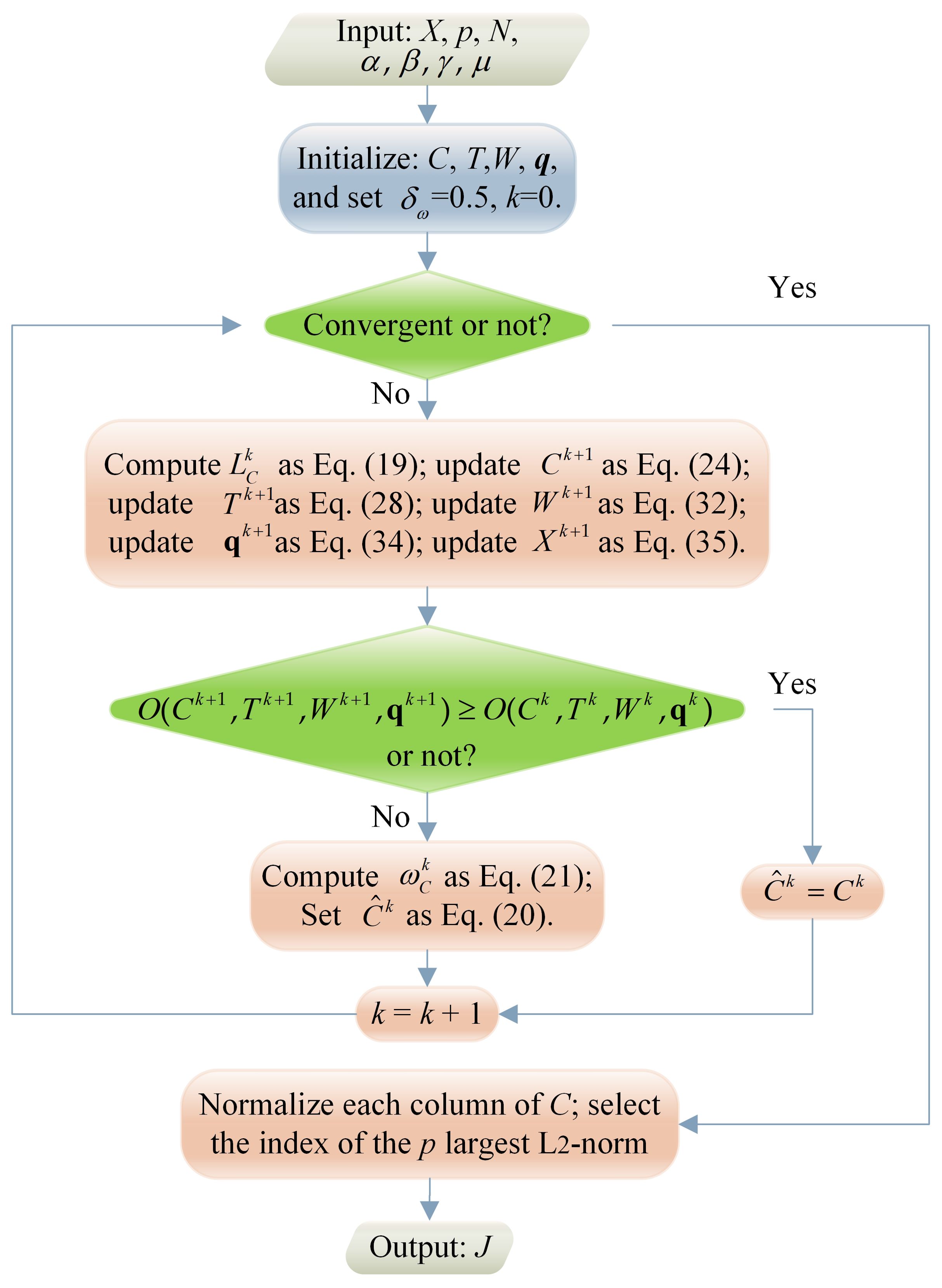
The entire iterative method proposed by BCU for solving Equations 18A–D is referred to as the Maximum Correntropy Criterion-based Robust Sensor Selection (MCC_RSS) algorithm. To elucidate the iterative process of the MCC_RSS algorithm more clearly, we present it in the form of a flowchart, as depicted in Figure 1. Herein, the output J represents the locations of selected sensors. For the sake of clarity, the total objective function in Equations 18A-D is expressed as follows:

Figure 1

Figure 1. Flowchart of MCC_RSS algorithm.

$\begin{array}{ll}O(C,T,W,q)=F(C,T,W,q)-\alpha {\Vert C\Vert }_{2,1}-E(W)& (36)\end{array}$

4.3 Theoretical analysis

4.3.1 Convergence analysis

To facilitate the convergence analysis, we present Theorem 2 and Lemma 1 as follows:

Lemma 1: At k-th iteration with fixed C and T, the solutions of W in Equation 32 are global optimal.

Proof: The W obtained by Equation 32 is the global optimal because it is solved by Lagrange multiplier method and the Equation 29 is convex with the fixed C and T.

Theorem 2: The sequence of $\{O(C^k,T^k,W^k,q^k)\}$, which is generated by the whole objective function in Equation 36 converges monotonically.

Proof: According to the BCU principle and Lemma 1, in the process of iterative optimization, we have:

$\begin{array}{ll}\begin{array}{l}\{O(C^k,T^k,W^k,q^k)\}\le \{O(C^{k+1},T^k,W^k,q^k)\}\le \{O(C^{k+1},T^{k+1},W^k,q^k)\}\\ \le \{O(C^{k+1},T^{k+1},W^{k+1},q^k)\}\le \{O(C^{k+1},T^{k+1},W^{k+1},q^{k+1})\}\end{array}& (37)\end{array}$

During each iteration, the energy of the objective function progressively increases through four sequential updates. Additionally, the objective function has an upper bound. Consequently, the MCC_RSS algorithm exhibits monotonic convergence.

4.3.2 Computational complexity

For the MCC_RSS algorithm, its computational complexity is determined by the number of samples m, the number of location features n in the original data matrix X, and the number of sensors to be selected p. The complexity of each variable update process is as follows:

Update sensor selective matrix C: $n{p}^2+n{m}^2+m^2+nm+n^2+n^3$

Update transformation matrix T: $pm+p^2+p^3+2np$

Update noise weight matrix W: $n^2+2nm$

Update variable q and X: $2nm+n{m}^2$Disregarding the sparsity of the original data matrix X, and by omitting the lower-order terms, the resultant time complexity is given by: $O(n^3+n{m}^2+n{p}^2+p^3)$.

5 Experimental evaluation and results

The MCC_RSS algorithm we proposed is compared with the QR-based sensor selection outlined in (Manohar et al., 2018), POD, and two random selection method. In these methods, data reconstruction is carried out by SVD basis (RS) and sparse representation [SR (Callaham et al., 2019)] respectively. To better demonstrate the robustness of the MCC_RSS method, we also compared the proposed algorithm with the MSE_RSS method [where MSE refers to the use of the Frobenius norm to evaluate the difference between the original data and the reconstructed data as in (Zhang et al., 2024)].

5.1 Dataset and experimental description

5.1.1 Datasets description

5.1.1.1 Ocean temperature

The ocean temperature data utilized in this study is derived from the IAP Global Ocean Temperature Dataset of version IAPv4 (Cheng et al., 2024a) provided by Institute of Atmospheric Physics (IAP), Chinese Academy of Sciences. This dataset includes bias-corrected data from various observational systems within the World Ocean Database as well as data obtained through model simulations by research group of IAP (Cheng and Jiang, 2016; Cheng et al., 2017). Together, these ensemble data constitute the full-state global ocean temperature data. Due to the extensive matrix operations involved in the algorithm and the limitations of our computer memory, a subset of the dataset was selected. Specifically, ocean temperature data from the North Pacific region was used here, with a geographical range of 65°N latitude to 10° S latitude, and 78°W longitude to 99°E longitude. The spatial resolution accuracy is 1°×1°, encompassing a total of 10,188 geographical coordinates as the sensor selection locations. In this study, sea surface temperature at vertical levels of 0m is used to conduct the experiments. In addition, the temporal resolution is monthly, with a total of 996 samples spanning from 1940 to 2022. Of these, the first 800 samples are used as the training dataset, and the remaining samples are used as the test dataset.

5.1.1.2 Ocean salinity

The ocean salinity data utilized in this study is also derived from the IAP Global Ocean Salinity Dataset (Cheng et al., 2024b). This dataset also includes bias-corrected data from the World Ocean Database and the IAP research group, as well as model simulation data (Cheng and Jiang, 2016; Cheng et al., 2020). Similar to the temperature data, salinity data from the North Pacific region, sharing the same geographical range, were extracted. The geospatial resolution is 1°×1°. This ocean salinity dataset encompasses 41 vertical levels ranging from 0 to 2000 meters. For this experiment, the salinity data from the first vertical level were used. The temporal resolution of this dataset is monthly, spanning from January 1940 to December 2021, comprising a total of 984 samples. Of these, the first 800 samples are used as training data, while the remaining samples are used as test data.

5.1.2 Quality of reconstruction

The performance of the proposed method is evaluated by reconstruction errors, which are represented as follows:

$\begin{array}{ll}{R}_{error}=\frac{{\Vert Test-\widehat{T}est\Vert }_2}{{\Vert Test\Vert }_2}& (38)\end{array}$

Wherein $Test$ is input test data from the test set, $\widehat{T}est$ is reconstructed by T from Equation 28 and the sensor’s measurement data $Y_{test}=C_J\times Test$, as $\widehat{T}est=T\times Y_{test}$. J is obtained from the sensor selection methods and $C_J$ is the corresponding sensor selection matrix.

5.1.3 Experimental setting

The hardware and software environment used in the experiment is shown in Table 1.

Table 1

Table 1. Experimental environment.

The specific parameter settings for the MCC_RSS algorithm are as follows: α=1×10⁶, β=1×10^-5, γ=1×10^-4, μ=1×10^-4, with the maximum number of iterations set to 400. During the execution of the MCC_RSS algorithm, the data is first normalized, followed by iterative updates of each subproblem solution based on BCU. The selection of these parameters is determined according to the algorithm’s iterative process. Specifically, inappropriate parameters can lead to non-convergence of the objective function or premature termination of iterations. For instance, the value of α affects the solution process of Equation 23; an unsuitable α will prevent effective updates of matrix C. We determined the specific value of α by observing the algorithm’s iterative process during experiments. Similarly, the values of β and γ influence the solution of the weight matrix W. Inappropriate values can cause the elements w_ij of Equation 32 to quickly converge to infinity or a constant, such as 1/2 (this conclusion can be easily derived by analyzing the relative relationship between β and γ in Equation 32). The value of μ is selected based on the overall distribution range of the objective function, ensuring it does not affect the convergence speed of the objective function value. Finally, among several alternative parameter combinations, the aforementioned parameters were selected as they exhibited the lowest error in the absence of noise.

To compare the robustness of different methods, we introduced varying proportions of outliers into the training data to simulate the loss conditions of actual oceanographic data. Considering the impact of non-Gaussian noise, we use the α-stable distribution to simulate heavy-tailed non-Gaussian noise, setting the signal-to-noise ratio parameter to 60. The alpha value (denoted as α₀ to avoid confusion with the model parameter α) is used to control the magnitude of the heavy tail, with α₀ set to1.

In the following experiments, Po=20% indicates that the proportion of outliers is 20%. Meanwhile, Sn=60 means that the signal-to-noise ratio of non-Gaussian noise is 60.

5.2 Reconstruction for ocean temperature

5.2.1 Compared with comparative methods

5.2.1.1 Reconstruction for different test snapshot

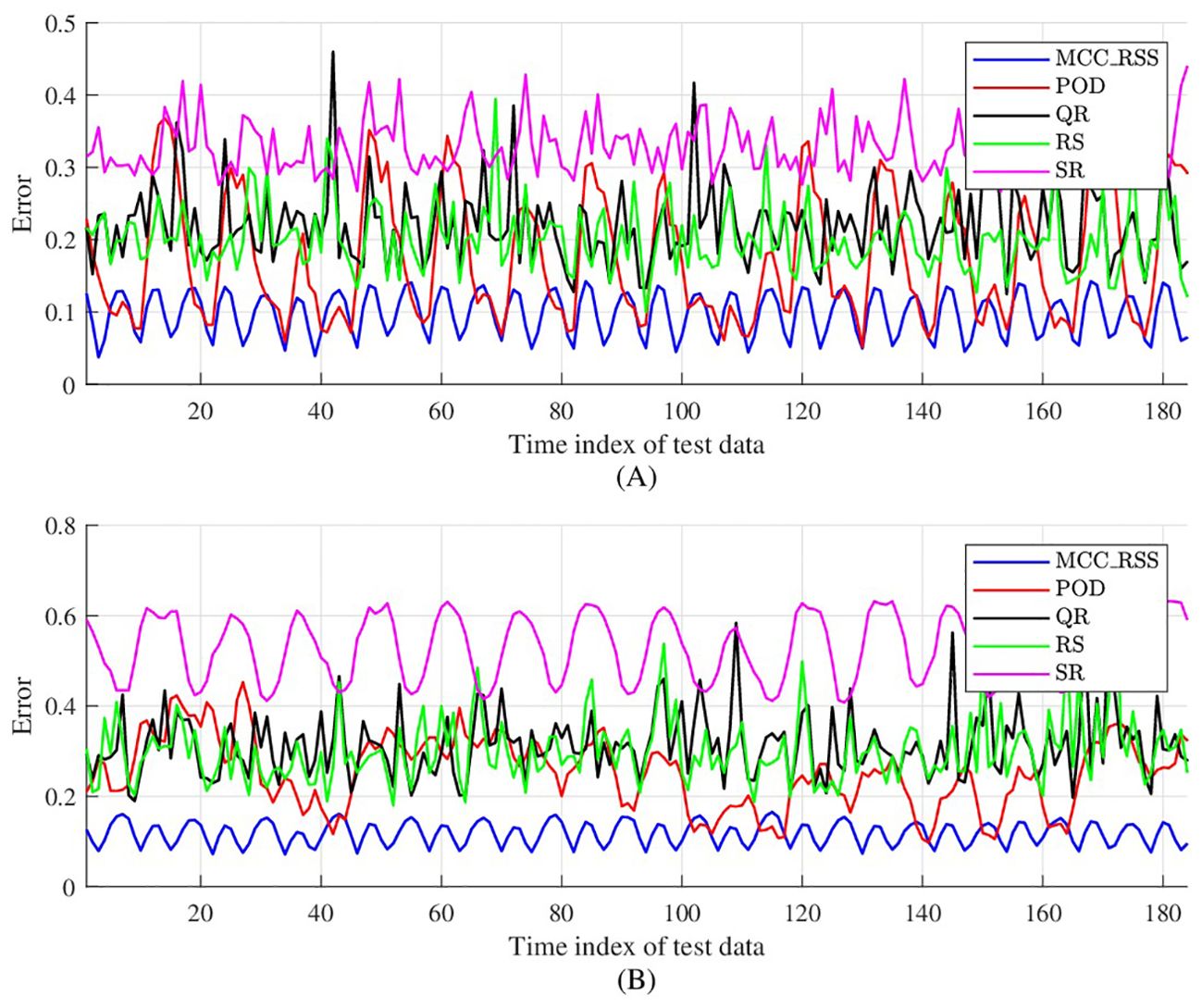
Figure 2 illustrates the comparison of reconstruction errors between the proposed method and the comparative methods for different snapshots in the test set. The number of selected sensors is set to 10. Due to the presence of random components in the comparative methods, each baseline method was executed 10 times, and the median error of the results was taken for comparison. Referring to Figure 2A, when there are outliers and noise in the training data, the reconstruction errors of the comparative methods increase rapidly. This indicates that the effectiveness of the QR and SR methods in the comparative methods is highly dependent on the quality of the training dataset. In contrast, the proposed MCC_RSS method can still minimize the impact of noise and maintain a low reconstruction error even in the presence of outliers and noise, achieving relatively stable reconstruction of test snapshots. Referring to Figure 2B, when the proportion of outliers in the training data increases and noise is still present, the proposed MCC_RSS method still exhibits the lowest reconstruction error compared to the comparative methods. Although the reconstruction error increases slightly compared to the case with weaker noise, the overall difference is small. This fully demonstrates that the proposed MCC_RSS method is minimally affected by noise in the training dataset during data reconstruction, and its sparse sensor selection process has good robustness.

Figure 2

Figure 2. Reconstruction error for temperature comparation. (A) Po =20%, Sn=60; (B) Po =40%, Sn=60.

Figure 2 also illustrates that the reconstruction errors of different methods fluctuate over different time periods. Despite the varying degrees of noise contamination in the training data, the proposed MCC_RSS method effectively captures these temporal fluctuations with only 10 selected sensors, demonstrating superior stability.

5.2.1.2 Reconstruction for one test snapshot

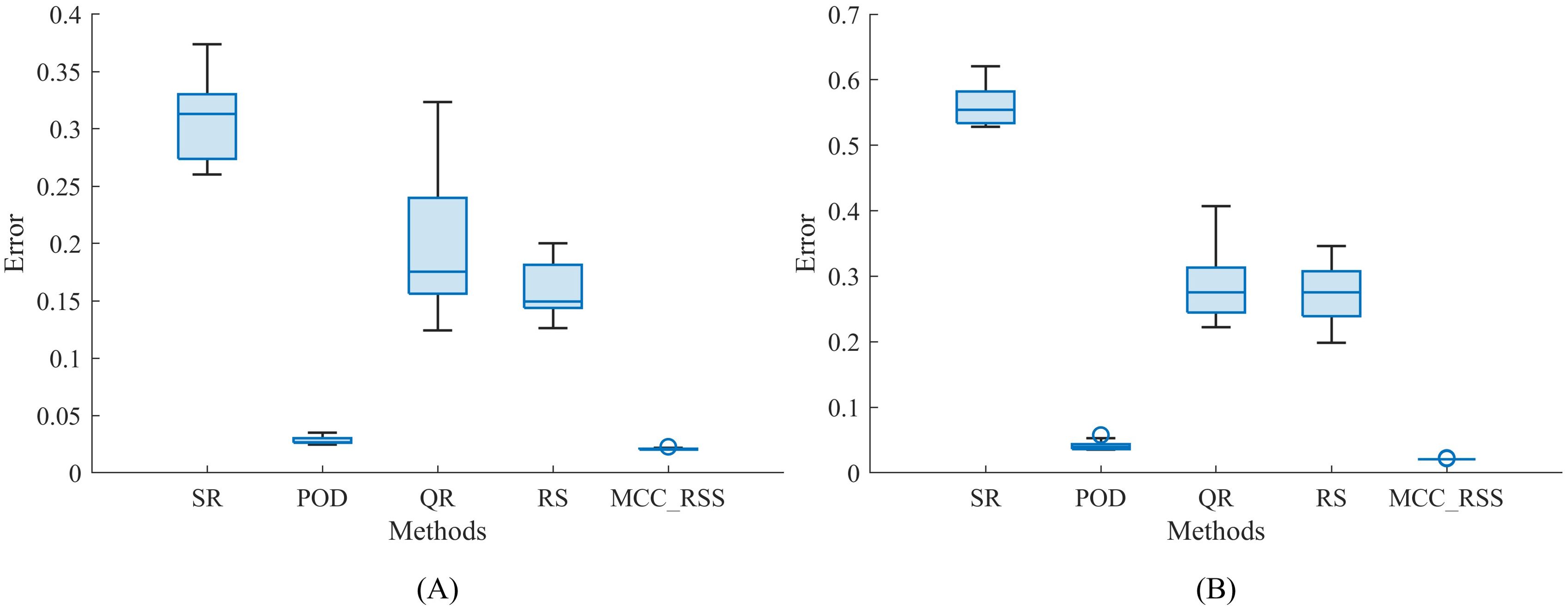
To better reflect the sensitivity of different methods to outliers, a 10-fold cross-validation approach was employed. The results for each method, based on a single snapshot with p = 10, are compared and illustrated in Figure 3. Figure 3A demonstrates that the overall reconstruction error of the proposed method is consistently than that of other methods after multiple validations. Figure 3B indicates that even as the number of outliers increases, the reconstruction error of the proposed method remains lower than that of the other three methods, with only the POD method occasionally achieving lower reconstruction error. However, overall, the results of the proposed method are highly stable, with outcomes remaining concentrated even after multiple experiments. In contrast, the results of the comparative method exhibit a larger distribution range and lack stability across multiple validations. This stability is primarily due to the iterative optimization algorithm proposed in this paper, which focuses on gradually approaching the optimal solution until the algorithm termination condition is met. In the comparative method, the reconstructing based on the basis or orthogonal basis of SVD decomposition is significantly influenced by the data itself, leading to the instability of the solution.

Figure 3

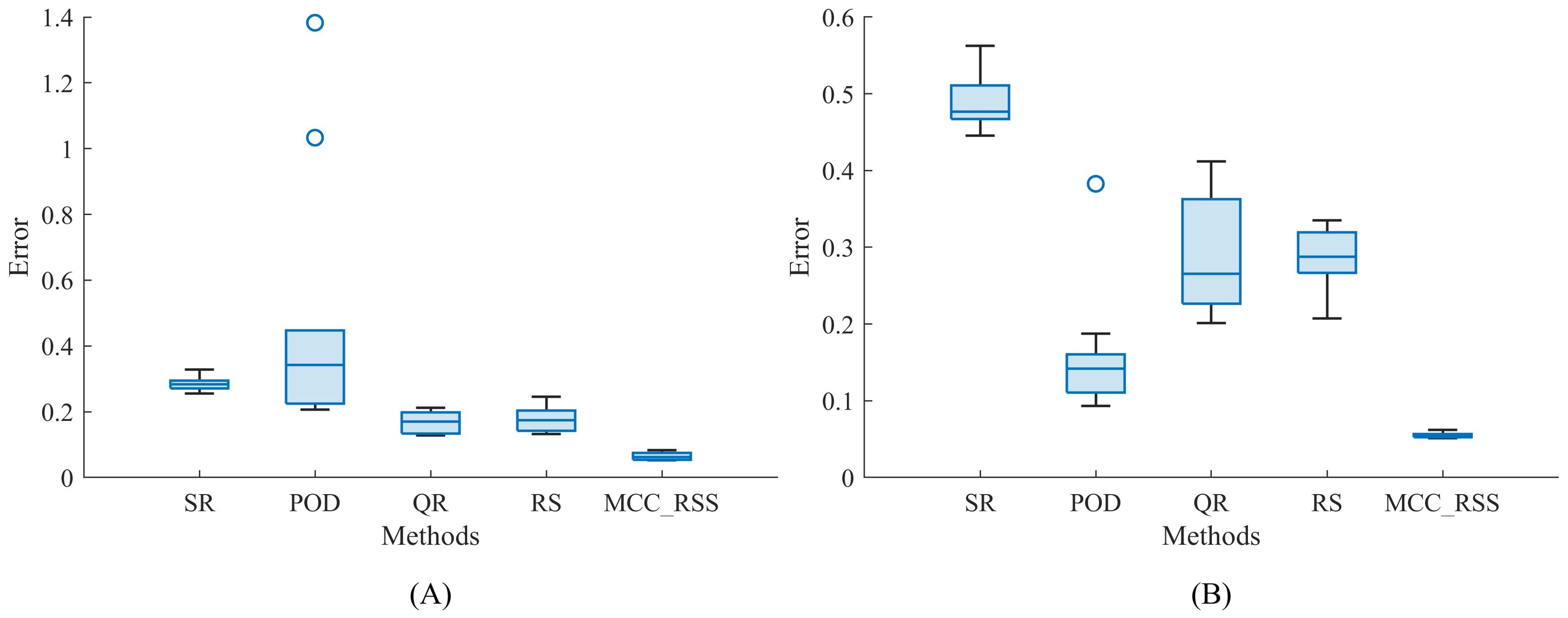
Figure 3. Reconstruction error of temperature for a snapshot. (A) Po =20%, Sn=60; (B) Po =40%, Sn=60.

Based on Figure 4, we present a randomly selected snapshot from the test set along with the corresponding reconstruction maps using different methods. In this scenario, the outlier ratio is set to 20%, and the signal-to-noise ratio is 60. The red dots in each reconstruction map indicate the sensor locations selected by the respective method. As shown in Figure 4B, the method proposed in this paper can effectively reconstruct the sea surface temperature distribution in the North Pacific region using only 10 selected sensors for this snapshot. Among the compared methods, only the POD method can relatively reconstruct the temperature distribution for this snapshot, but it still contains numerous noise points. Naturally, the reconstruction results vary for different snapshots, as indicated by the numerical comparison of reconstruction errors mentioned above. Although the POD method performs relatively well for this particular snapshot, the numerical results demonstrate that its reconstruction error is still higher than that of the proposed method when only 10 sensors are selected, and its stability is compromised by the randomly chosen sensor locations.

Figure 4

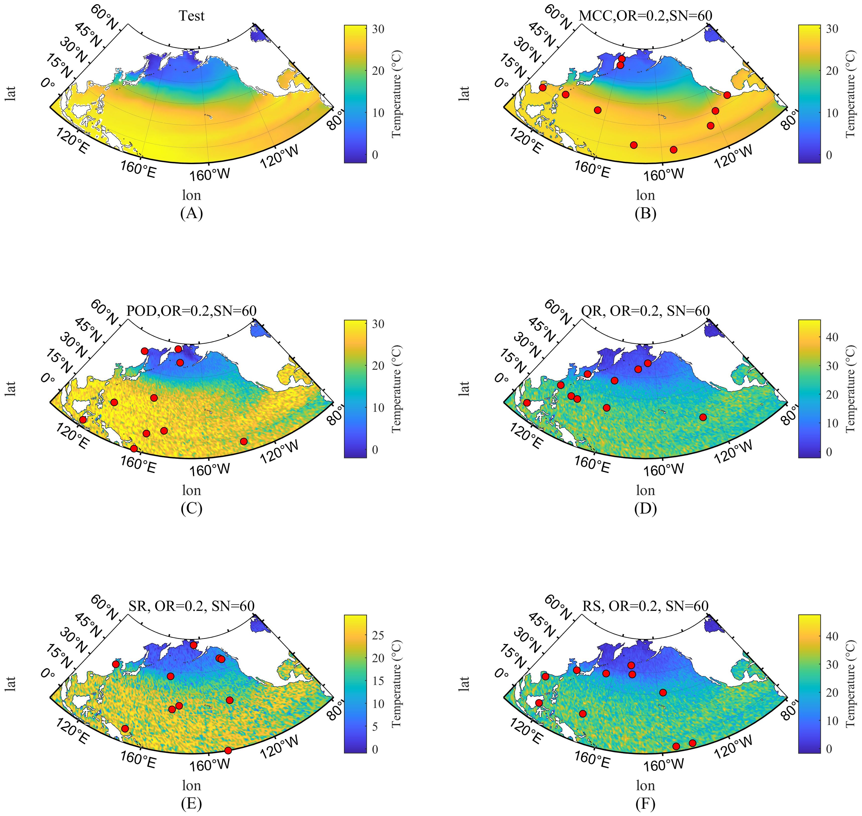
Figure 4. Reconstruction error of temperature for a snapshot. (A) Snapshot of test; (B) Reconstructed temperature by MCC_RSS; (C) Reconstructed temperature by POD; (D) Reconstructed temperature by QR; (E) Reconstructed temperature by SR; (F) Reconstructed temperature by RS.

5.2.1.3 Reconstruction error by different number of sensors

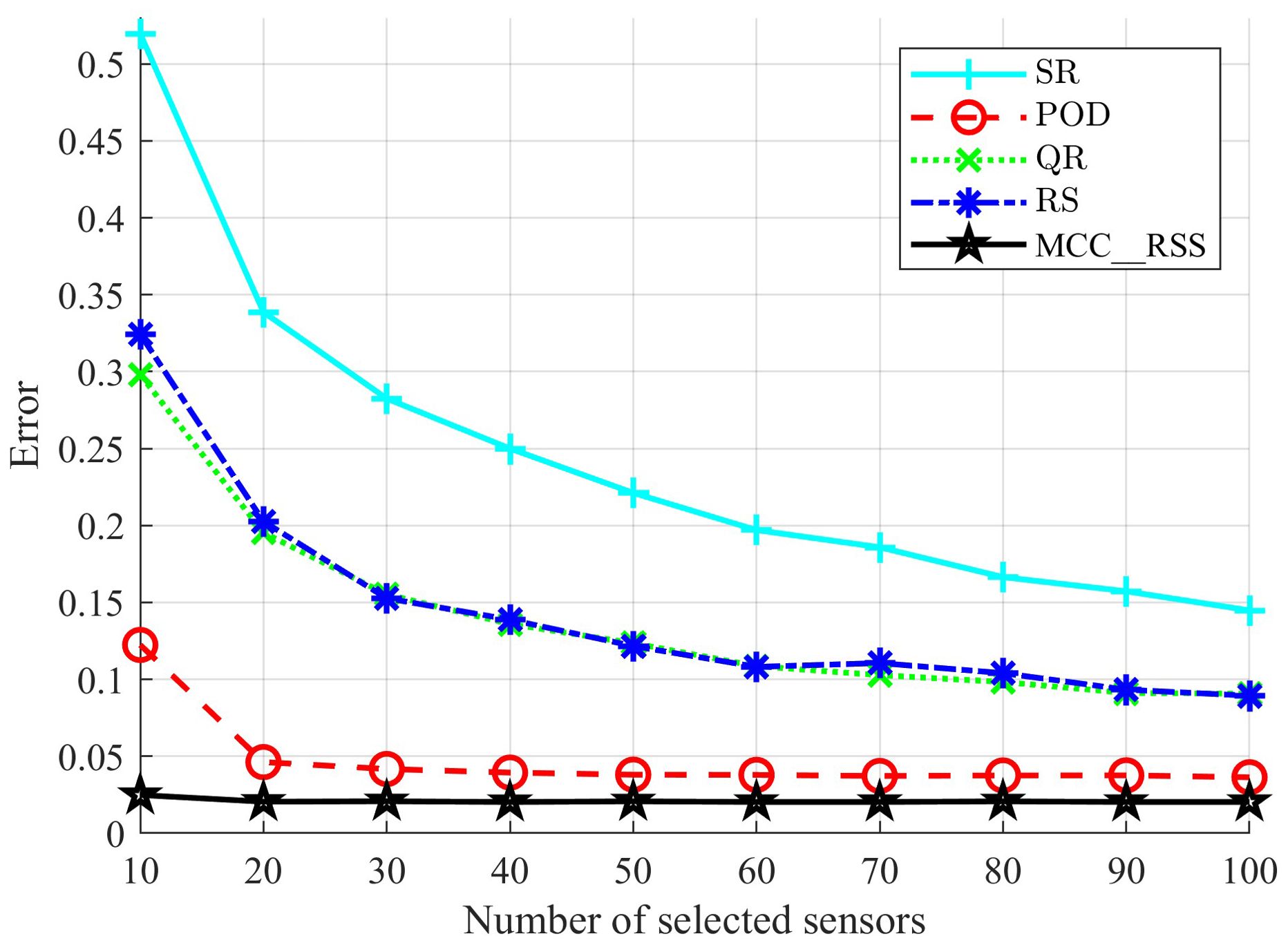
Figure 5 presents a comparison of reconstruction errors for different methods when varying the numbers of selected sensors, under noise conditions of Po=20% and Sn=60%. To mitigate the influence of random factors, the comparative methods were subjected to 10-fold cross-validation. The error comparison results in Figure 5 indicate that when the training data contains noise, the proposed MCC_RSS method consistently achieves significantly lower reconstruction errors than other comparative methods, regardless of the number of sensors selected. Additionally, while the reconstruction errors of the comparative methods decrease as the number of sensors increases, the reconstruction error obtained by the proposed method shows almost no significant change. The primary reason for this is that, in the proposed method, after obtaining a C matrix through subspace learning, the column indices (i.e., sensor locations) are determined by selecting the columns with the largest 2-norms for a given number of sensors. Therefore, once the training data is given, the low-dimensional subspace obtained through subspace learning is fixed, and selecting more sensors does not contribute additional useful information to the identified subspace. This results in the reconstruction error remaining nearly constant regardless of the number of sensors. Consequently, a very small number of sensors can still achieve good reconstruction performance. In contrast, the comparative methods increase the number of features used as the number of sensors increases, leading to a reduction in reconstruction error. Therefore, the proposed method is more suitable for scenarios requiring a limited number of sensors.

Figure 5

Figure 5. Reconstruction error of temperature by different number of sensors.

5.2.2 Compared with MSE_RSS methods

To better demonstrate the effectiveness of the MCC method in improving robustness, we compare the proposed MCC_RSS method with the MSE_RSS method, as shown in Figure 6. The primary difference between MSE_RSS and MCC_RSS lies in the measurement of the discrepancy between the original and reconstructed data, with MSE_RSS lacking the local geometric structure preservation term. The update formulas for Lipschitz constant of MSE_RSS are presented as: $L_C^k={\Vert A^k\Vert }_2^2{\Vert X\Vert }_2^2{\Vert W^k\Vert }_2$, where X remains unchanged during the iteration process.

Figure 6

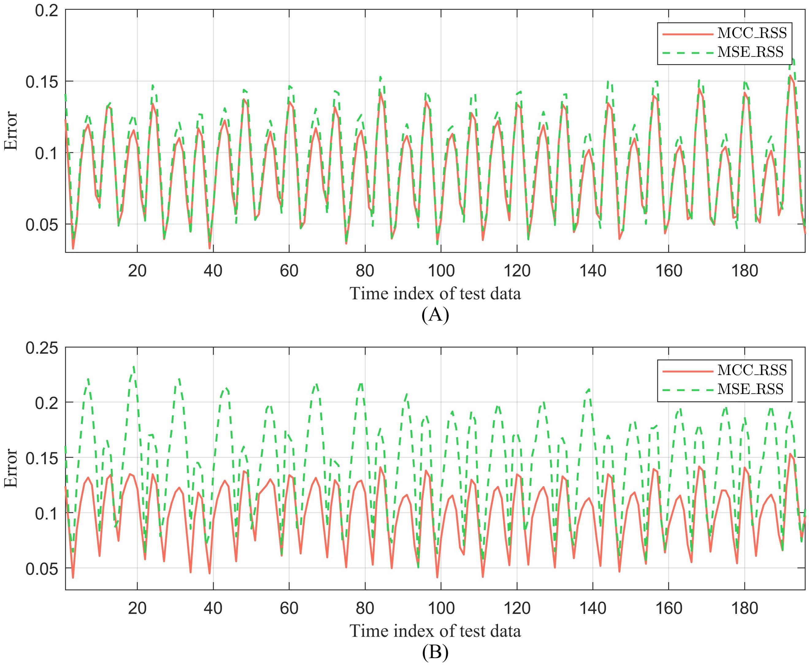
Figure 6. Comparison between MCC_RSS and MSE-RSS of ocean temperature. (A) No additional noise; (B) Po =20%, Sn=60.

The reconstruction error results shown in Figure 6A indicate that even for subspace learning on training data without added noise, the sensor subset selected by the proposed MCC_RSS method achieves superior data reconstruction performance compared to the MSE_RSS method. This is primarily because, even without additional noise in the ocean temperature training data, the original data inherently contains model noise introduced during the ocean data assimilation process. The sensor selection method based on MCC proposed in this paper can minimize the impact of such noise as much as possible. Furthermore, Figure 6B presents the reconstruction results of these two methods when the training data contains 40% outliers and non-Gaussian noise. The results demonstrate that, with more severe noise, the difference in reconstruction performance between the sensor subset selected by the proposed MCC_RSS method and the MSE_RSS method further increases. This indicates that the proposed MCC_RSS method, by using MCC as the measure of the difference between the original and reconstructed data, is better able to mitigate the impact of noise on the results when the training data contains noise.

5.3 Reconstruction for ocean salinity

5.3.1 Compared with comparative methods

5.3.1.1 Reconstruction for different test snapshot

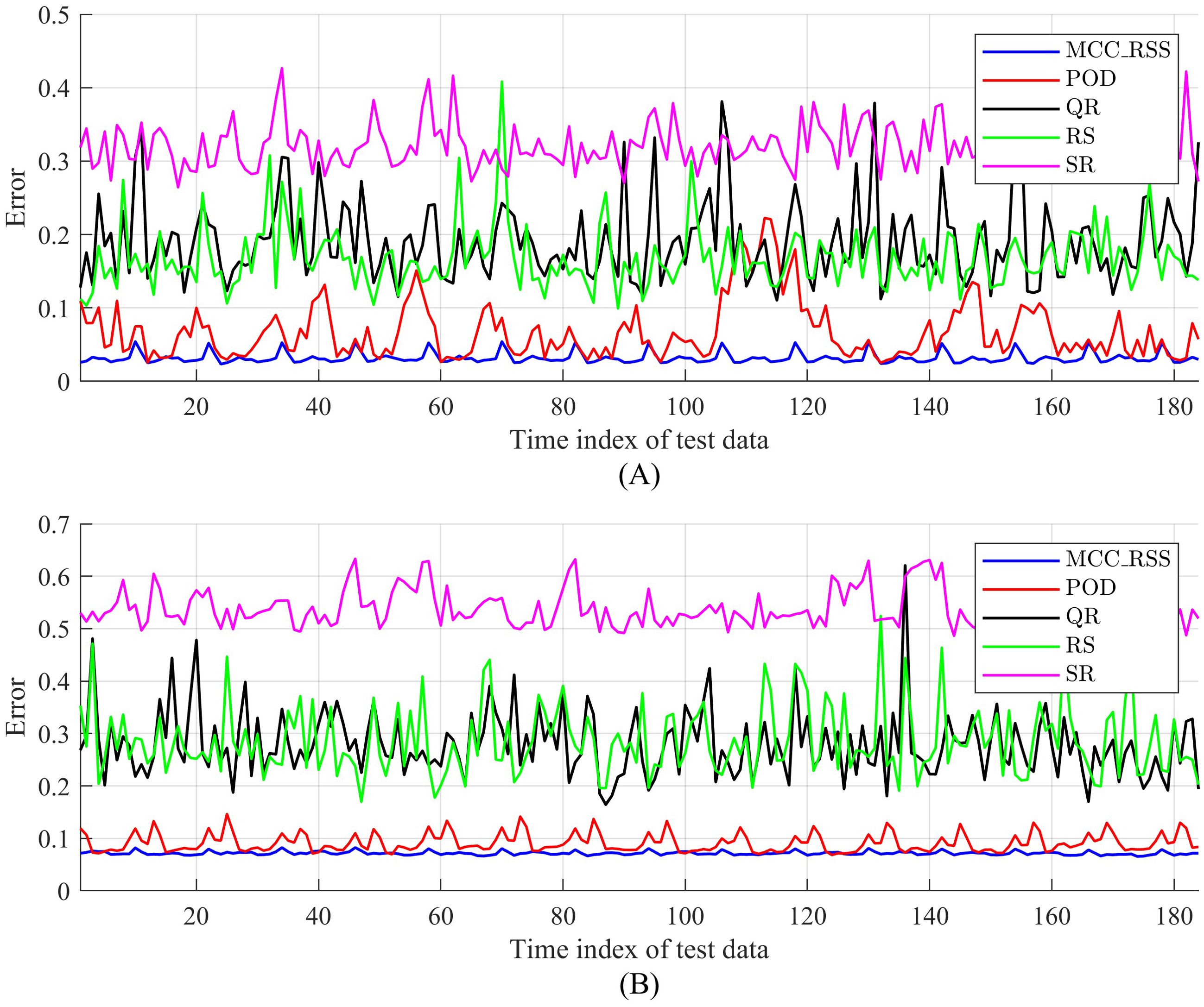
Figure 7 presents a comparison of the reconstruction errors between the proposed method and the comparative methods for ocean salinity data, with the number of sensors selected being 10. From Figures 7A, B, it can be observed that when the training data contains varying levels of noise, the reconstruction errors of the proposed MCC_RSS method are consistently lower than those of the comparative methods. Additionally, the reconstruction errors still reflect the periodicity of the ocean data to a certain extent. As the level of noise contamination in the training data increases, the reconstruction errors of all methods decrease. However, compared to the comparative methods, the decrease in reconstruction error for the proposed MCC_RSS method is less significant. This further demonstrates that, when selecting sensors for ocean salinity data, the proposed MCC_RSS method is less affected by the noise present in the data compared to the comparative methods.

Figure 7

Figure 7. Reconstruction error for salinity comparation. (A) Po =20%, Sn=60; (B) Po =40%, Sn=60.

5.3.1.2 Reconstruction for one test snapshot

Figure 8 presents a comparison of reconstruction error for a randomly selected sample (snapshot) using 10-fold cross-validation, with p=10. From Figures 8A, B, it can be observed that despite variations in outliers and noise distribution in the ocean salinity training data during multiple implementations of both the proposed method and the comparison method, the reconstruction error distribution of the proposed MCC_RSS method remains relatively concentrated, indicating better algorithm stability. In contrast, the reconstruction error distribution of the comparison method becomes more dispersed when the noise distribution in the training data changes. Additionally, the proposed method consistently achieves the lowest reconstruction error. This result further demonstrates that the MCC_RSS algorithm, based on MCC subspace learning, can iteratively learn a relatively stable low-dimensional subspace under different conditions, thereby ensuring that the selected subset of sensor measurements exhibits good robustness and achieves better data reconstruction.

Figure 8

Figure 8. Reconstruction error of salinity for a snapshot. (A) Po =20%, Sn=60; (B) Po =40%, Sn=60.

Figure 9 presents a comparison of the reconstruction effects of different methods on the aforementioned randomly selected snapshot, with the noise in the training data set to Po=20% and Sn=60%. The red dots indicate the positions of the sensors selected by the different methods. As shown in Figure 9B, the proposed MCC_RSS method achieves effective reconstruction of ocean salinity data with only a subset of 10 sensors, successfully capturing the main characteristics of the salinity distribution in the North Pacific region when compared to the test snapshot. The POD method, while slightly inferior to the proposed method, also generally reflects the main patterns of salinity distribution in the North Pacific region. However, the other three comparative methods fail to capture the salinity distribution characteristics with only a subset of 10 sensors. This indicates that, even with a certain level of noise in the training data and a limited number of sensors, the sensor subset selected by the proposed MCC_RSS method can still achieve effective data reconstruction.

Figure 9

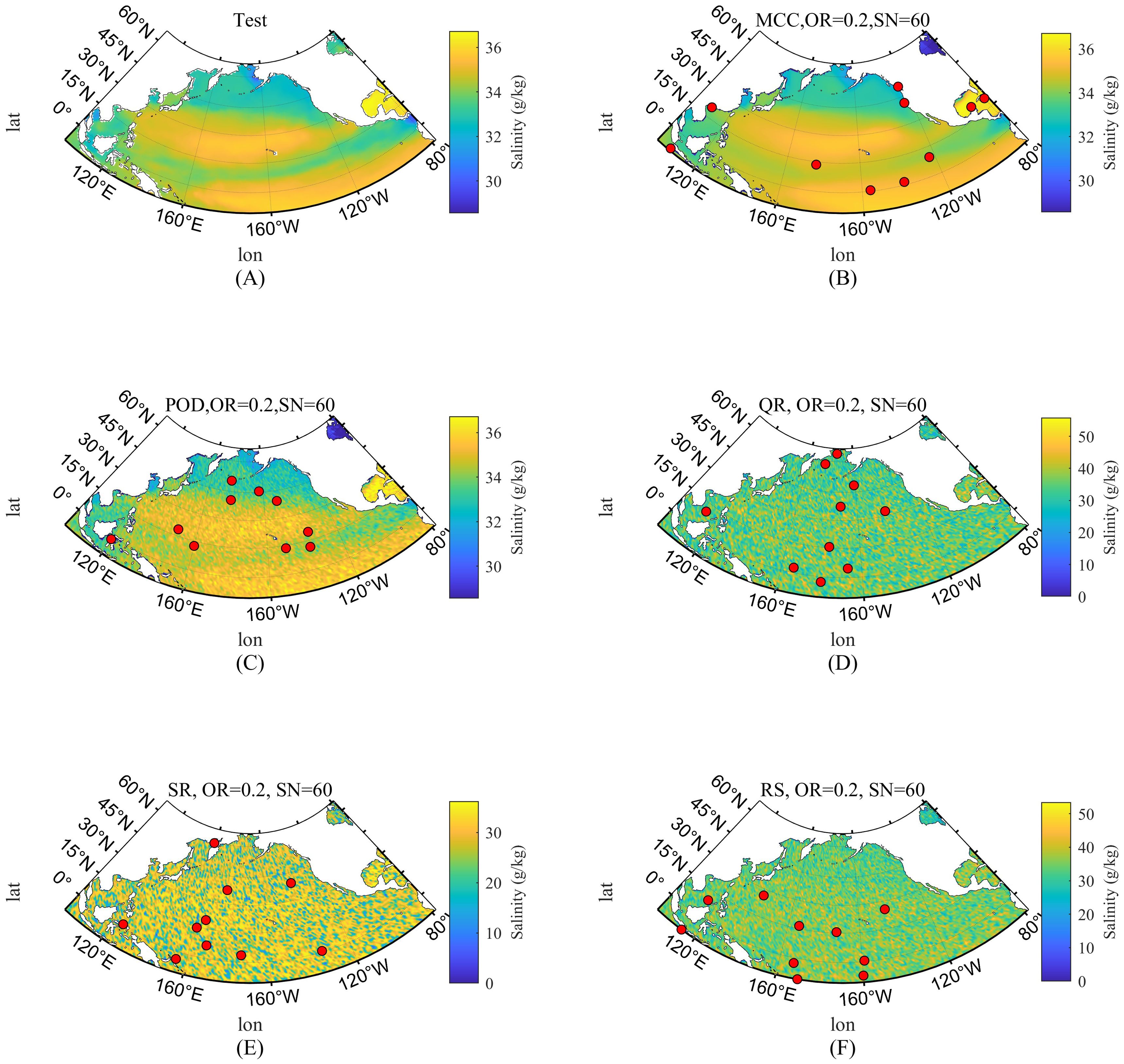
Figure 9. Reconstruction error of salinity for a snapshot. (A) Snapshot of test; (B) Reconstructed salinity by MCC_RSS; (C) Reconstructed salinity by POD; (D) Reconstructed salinity by QR; (E) Reconstructed salinity by SR; (F) Reconstructed salinity by RS.

5.3.1.3 Reconstruction error by different number of sensors

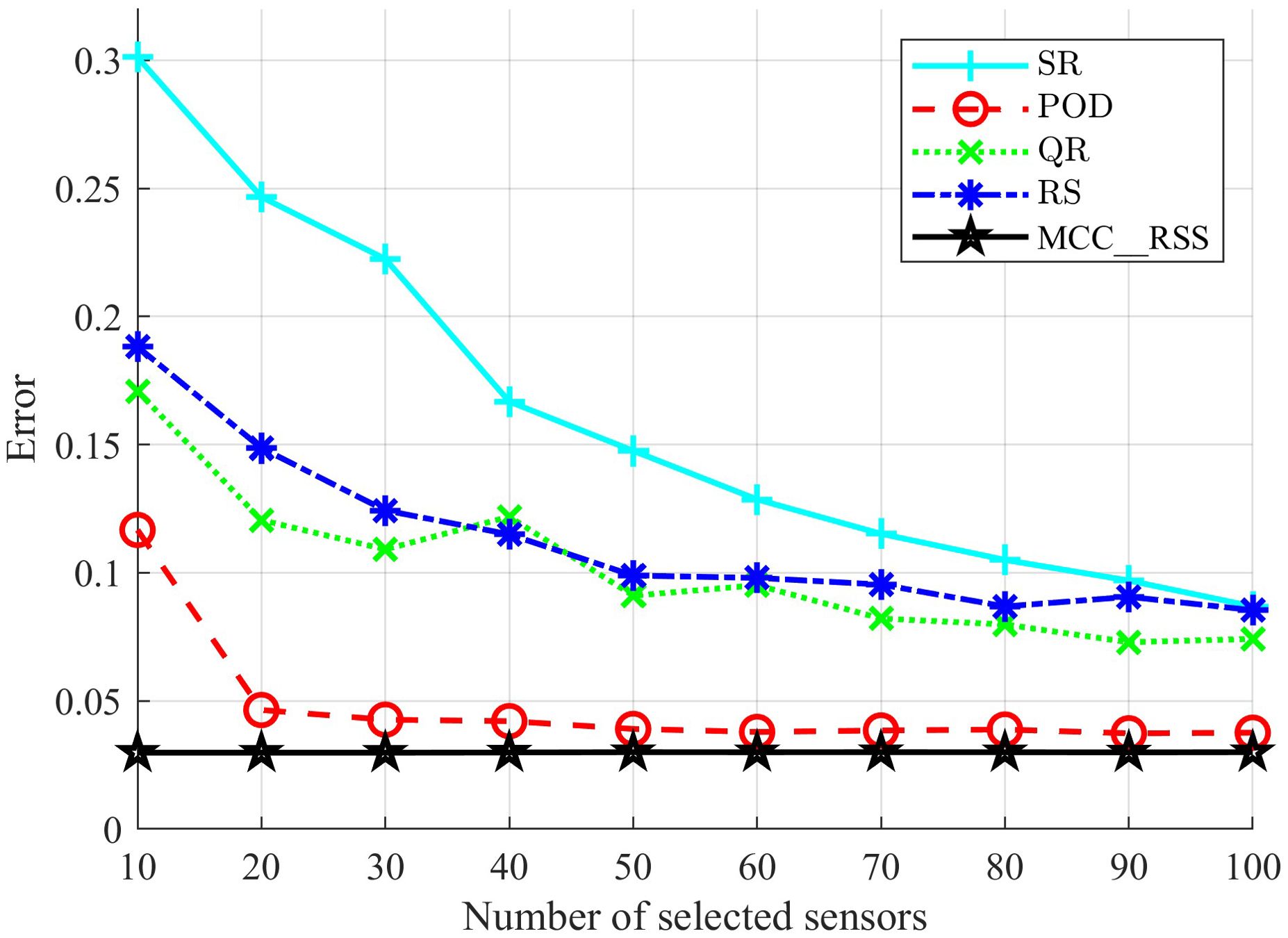
Figure 10 presents a comparison of the reconstruction errors for different methods when selecting varying numbers of sensors. The noise in the training data is set to Po=40% and Sn=60. As shown in the figure, the proposed MCC_RSS method consistently achieves the lowest reconstruction error compared to the comparative methods, regardless of the number of sensors selected. Additionally, as the number of sensors increases, the reconstruction error remains relatively stable. As previously mentioned, once the proposed MCC_RSS method determines the matrix C corresponding to the low-dimensional subspace, the indices of the selected sensors, regardless of their number, are derived from the entries of matrix C with the largest 2-norms of the columns. This selection process does not significantly alter the obtained subspace, further demonstrating that the low-dimensional subspace derived from the proposed method is relatively stable. Consequently, it is more suitable for scenarios with fewer sensors compared to the comparative methods.

Figure 10

Figure 10. Reconstruction error of salinity by different number of sensors.

In contrast, for the comparative methods, particularly the QR and RS methods, the reconstruction error decreases rapidly as the number of selected sensors increases. However, they are still significantly affected by noise, and their reconstruction errors are not as favorable as those of the proposed method. The SR method, which relies more heavily on the library established from the training data, is the most affected by noise. Comparatively, the POD method performs closer to the proposed method in terms of ocean salinity reconstruction and can reasonably reconstruct salinity data with different numbers of sensors. Nevertheless, its error remains significantly higher than that of the proposed method.

Therefore, utilizing the sensors selected by the proposed MCC_RSS method for data reconstruction can achieve more desirable results, particularly when the number of sensors is limited.

5.3.2 Compared with MSE_RSS methods

Figure 11 shows the experimental results of the proposed MCC_RSS method and the corresponding MSE_RSS method on global ocean salinity data, using 10 sensors. As shown in Figure 11A, when no additional noise is introduced to the training data, there is no significant difference in the reconstruction errors between the two methods. Differences are observed only in specific time samples, such as in the trough region between sample indices 100 and 140, where the error of the MCC_RSS method is smaller than that of the corresponding MSE_RSS method. In Figure 11B, when the training data contains noise, it is evident that the overall fluctuation of the reconstruction error of the MCC_RSS method is significantly smaller than that of the MSE_RSS method. The average error of the MCC_RSS method is 0.0375, while the average error of the MSE_RSS method is 0.0391. This further demonstrates that the proposed method can more effectively mitigate the impact of noise.

Figure 11

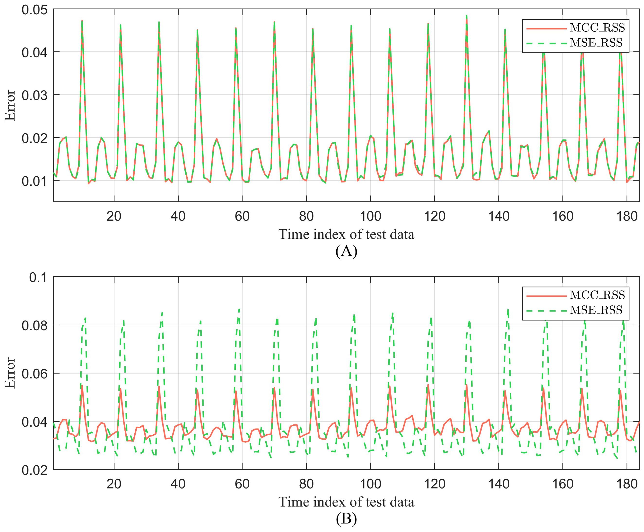
Figure 11. Comparison between MCC_RSS and MSE-RSS of ocean salinity. (A) No additional noise; (B) Po =20%, Sn=60.

6 Conclusion and discussion

Considering the distinct low-rank characteristics of ocean data, we explored how to optimally utilize subspace learning methods to derive a more reasonable low-dimensional subspace of high-dimensional ocean data. This approach facilitates the selection of low-dimensional measurements from sensors that better meet the requirements. Based on this premise, we develop a robust sensor selection method that establishes an evaluation function based on the Maximum Correntropy Criterion (MCC) and selects sensor subsets to reconstruct the full state ocean data through subspace learning. Compared to the Euclidean distance used in existing methods, MCC demonstrates superior robustness in evaluating the discrepancies between reconstructed data and original data, particularly in the presence of varying levels of noise in the original data. The model also incorporates noise weighting and optimizes noise distribution using entropy terms, effectively controlling sparse severe noise and mitigating the impact of non-Gaussian noise and outliers. The use of noise weighting in the proposed method allows for better identification of varying levels of noise during the subspace learning process. This reduces the impact on the learned subspace, resulting in more stable reconstruction outcomes for sensor selection under different noise conditions.

Furthermore, the integration of the local geometric structure of data samples further enhances the reconstruction accuracy achieved by the selected sensors. By minimizing the similarity of the selected sensor measurement subset through the graph Laplacian matrix between samples, the reconstruction capability of the selected sensors for the full state data is further improved. To better solve the model’s evaluation function, the half-quadratic BCU method was employed, effectively addressing the challenge of solving the non-convex parts of the objective function. During the iterative solving process, the selection matrix, transformation matrix, and noise weighting matrix continuously evolve towards the optimal solution. This ultimately results in the learned low-dimensional subspace, along with the corresponding selection and transformation matrices, achieving superior data reconstruction outcomes. Additionally, the model effectively converges to the optimal solution with a low number of iterations.

Compared to the benchmark methods, our approach performs better and yields highly robust solutions under varying noise conditions. Specifically, the proposed method demonstrates that even with data containing different levels of noise, it can achieve effective data reconstruction using a smaller number of sensors. This makes it particularly suitable for ocean data reconstruction where the number of sensors is limited. This provides a valuable reference for future ocean environment monitoring systems on how to deploy fewer sensors more efficiently.

In our future work, we will explore how to improve the method proposed in this paper to reduce its computational complexity. For example, after preliminary screening of location features using statistical methods such as variance analysis and correlation coefficients, BCU iterative solving can be performed, or location features can be grouped and optimized separately before combining the results. For the parameter selection, we will also explore more scientific methods, such as grid search and Bayesian methods, to obtain parameter values that can achieve the optimal convergence results of the objective function. In addition, the method proposed in this paper does not make a significant contribution to the results when the number of sensors increases. Therefore, with the increase in the number of selected sensors, further exploration is needed to obtain a better low-dimensional subspace that can introduce more effective information. Potential improvements include incorporating oceanographic knowledge to screen location features, thereby identifying the most valuable candidate locations for monitoring. Alternatively, oceanographic models can be used to assess the value of each location feature, facilitating the optimization of a data-driven sensor selection model.

Data availability statement

The original contributions presented in the study are included in the article/supplementary material. Further inquiries can be directed to the corresponding author.

Author contributions

QZ: Conceptualization, Formal Analysis, Methodology, Validation, Writing – original draft, Writing – review & editing. HW: Funding acquisition, Project administration, Supervision, Writing – review & editing. LL: Investigation, Writing – review & editing. XM: Formal Analysis, Writing – review & editing. JX: Writing – review & editing, Supervision.

Funding

The author(s) declare that financial support was received for the research, authorship, and/or publication of this article. This research was funded by the National Natural Science Foundation of China (Grant Nos. 52331012, 52071200, 52201401, 52201403, and 52102397), in part by the National Key Research and Development Program (Grant No. 2021YFC2801002), in part by the Shanghai Committee of Science and Technology, China (Grant No. 23010502000), in part by the Chenguang Program of Shanghai Education Development Foundation and Shanghai Municipal Education Commission (No. 23CGA61), in part by the Top-Notch Innovative Program for Postgraduates of Shanghai Maritime University under Grant 2022YBR012.

Acknowledgments

We acknowledge the use of ChatAI (version Chat GPT 4o) for translation purposes in this study.

Conflict of interest

The authors declare that the research was conducted in the absence of any commercial or financial relationships that could be construed as a potential conflict of interest.

Publisher’s note

All claims expressed in this article are solely those of the authors and do not necessarily represent those of their affiliated organizations, or those of the publisher, the editors and the reviewers. Any product that may be evaluated in this article, or claim that may be made by its manufacturer, is not guaranteed or endorsed by the publisher.

References

Callaham J. L., Maeda K., Brunton S. L. (2019). Robust flow reconstruction from limited measurements via sparse representation. Phys. Rev. Fluids. 4. doi: 10.1103/PhysRevFluids.4.103907

Crossref Full Text | Google Scholar

Carmi A., Gurfil P. (2013). Sensor selection via compressed sensing. Automatica (Oxf). 49, 3304–3314. doi: 10.1016/j.automatica.2013.08.032

Crossref Full Text | Google Scholar

Chamon L. F. O., Pappas G. J., Ribeiro A. (2021). Approximate supermodularity of kalman filter sensor selection. IEEE Trans. Automat. Contr. 66, 49–63. doi: 10.1109/TAC.9

Crossref Full Text | Google Scholar

Cheng L., Trenberth K. E., Fasullo J. T., Boyer T., Abraham J. P., Zhu J., et al. (2024a). Data from: Institute of Atmospheric Physics, Chinese Academy of Sciences. Available online at: http://www.ocean.iap.ac.cn/ftp/cheng/IAPv4_IAP_Temperature_gridded_1month_netcdf/ (Accessed June 02, 2024).

Google Scholar

Cheng L., Trenberth K. E., Gruber N., Abraham J. P., Fasullo J. T., Li G., et al. (2024b). Data from: Institute of Atmospheric Physics, Chinese Academy of Sciences. Available online at: http://www.ocean.iap.ac.cn/ftp/cheng/CZ16_v0_IAP_Salinity_gridded_1month_netcdf/ (Accessed June 2, 2024).

Google Scholar

Cheng L., Jiang Z. (2016). Benefits of CMIP5 multimodel ensemble in reconstructing historical ocean subsurface temperature variations. J. Clim. 29, 5393–5416. doi: 10.1175/JCLI-D-15-0730.1

Crossref Full Text | Google Scholar

Cheng L., Trenberth K. E., Fasullo J. T., Boyer T., Abraham J. P., Zhu J. (2017). Improved estimates of ocean heat content from 1960 to 2015. Sci. Adv. 3. doi: 10.1126/sciadv.1601545

PubMed Abstract | Crossref Full Text | Google Scholar

Cheng L., Trenberth K. E., Gruber N., Abraham J. P., Fasullo J. T., Li G., et al. (2020). Improved estimates of changes in upper ocean salinity and the hydrological cycle. J. Clim. 33, 10357–10381. doi: 10.1175/JCLI-D-20-0366.1

Crossref Full Text | Google Scholar

Chepuri S. P., Leus G. (2015). Sparsity-promoting sensor selection for non-linear measurement models. IEEE Trans. Signal Process. 63, 684–698. doi: 10.1109/TSP.2014.2379662

Crossref Full Text | Google Scholar

Dubois P., Gomez T., Planckaert L., Perret L. (2022). Machine learning for fluid flow reconstruction from limited measurements. J. Comput. Phys. 448. doi: 10.1016/j.jcp.2021.110733

Crossref Full Text | Google Scholar

Emily C., Steven L. B., Kutz J. N. (2020). Multi-fidelity sensor selection-Greedy algorithms to place cheap and expensive sensors with cost constraints. IEEE Sens. J. 21, 600–611. doi: 10.1109/JSEN.2020.3013094

Crossref Full Text | Google Scholar

Erichson N. B., Mathelin L., Yao Z., Brunton S. L., Mahoney M. W., Kutz J. N. (2020). Shallow neural networks for fluid flow reconstruction with limited sensors. Pro. Roy Soc A. 476. doi: 10.1098/rspa.2020.0097

Crossref Full Text | Google Scholar

Fukami K., Maulik R., Ramachandra N., Fukagata K., Taira K. (2021). Global field reconstruction from sparse sensors with Voronoi tessellation-assisted deep learning. Nat. Mach. Intell. 3, 945–951. doi: 10.1038/s42256-021-00402-2

Crossref Full Text | Google Scholar

Ghosh S., De S., Chatterjee S., Portmann M. (2021). Learning-based adaptive sensor selection framework for multi-sensing WSN. IEEE Sens. J. 21, 13551–13563. doi: 10.1109/JSEN.2021.3069264

Crossref Full Text | Google Scholar

Guo X., Lin Z. (2018). Low-rank matrix recovery via robust outlier estimation. IEEE Trans. Image Process. 27, 5316–5327. doi: 10.1109/TIP.2018.2855421

Crossref Full Text | Google Scholar

He R., Hu B., Yuan X., Wang L. (2014). “Correntropy and linear representation,” in Robust recognition via information theoretic learning (SpringerBriefs in Computer Science: Springer, Cham), 45–60.

Google Scholar

He Y., Wang F., Wang S., Cao J., Chen B. (2019). Maximum correntropy adaptation approach for robust compressive sensing reconstruction. Inform. Sci. 480, 381–402. doi: 10.1016/j.ins.2018.12.039

Crossref Full Text | Google Scholar

Jayaraman B., Al Mamun S. M. A., Lu C. (2019). Interplay of sensor quantity, placement and system dimension in POD-based sparse reconstruction of fluid flows. Fluids. 4. doi: 10.3390/fluids4020109

Crossref Full Text | Google Scholar

Jayaraman B., Mamun S. M. A. A. (2020). On data-driven sparse sensing and linear estimation of fluid flows. Sensors. 20. doi: 10.3390/s20133752

Crossref Full Text | Google Scholar

Joneidi M., Zaeemzadeh A., Shahrasbi B., Qi G.-J., Rahnavard N. (2020). E-optimal sensor selection for compressive sensing-based purposes. IEEE Trans. Big Data. 6, 51–65. doi: 10.1109/TBigData.6687317

Crossref Full Text | Google Scholar

Joshi S., Boyd S. (2009). Sensor selection via convex optimization. IEEE Trans. Signal Process. 57, 451–462. doi: 10.1109/TSP.2008.2007095

Crossref Full Text | Google Scholar

Kalinić H., Ćatipović L., Matić F. (2022). Optimal sensor placement using learning models—A mediterranean case study. Remote Sens. 14. doi: 10.3390/rs14132989

Crossref Full Text | Google Scholar

Khokhlov I., Pudage A., Reznik L. (2019).Sensor selection optimization with genetic algorithms. In: 2019 IEEE SENSORS (Montreal, QC, Canada) (Accessed 27-30 October 2019). 2019 IEEE SENSORS.

Google Scholar

Krause A., Singh A., Guestrin C. (2008). Near-optimal sensor placements in gaussian processes theory, efficient algorithms and empirical studies. J. Mach. Learn. Res. 9, 235–284. doi: 10.5555/1390681.1390689

Crossref Full Text | Google Scholar

Lin X., Chowdhury A., Wang X., Terejanu G. (2019). Approximate computational approaches for Bayesian sensor placement in high dimensions. Inform Fusion. 46, 193–205. doi: 10.1016/j.inffus.2018.06.006

Crossref Full Text | Google Scholar

Liu W., Pokharel P. P., Principe J. C. (2007). Correntropy: properties and applications in non-gaussian signal processing. IEEE Trans. Signal Process. 55, 5286–5298. doi: 10.1109/TSP.2007.896065

Crossref Full Text | Google Scholar

Liu X., Wang L., Zhang J., Yin J., Liu H. (2014). Global and local structure preservation for feature selection. IEEE Trans. Neural Netw. Learn Syst. 25, 1083–1095. doi: 10.1109/TNNLS.2013.2287275

Crossref Full Text | Google Scholar

Manohar K., Brunton B. W., Kutz J. N., Brunton S. L. (2018). Data-driven sparse sensor placement for reconstruction: demonstrating the benefits of exploiting known patterns. IEEE Control Syst. 38, 63–86. doi: 10.1109/MCS.2018.2810460

Crossref Full Text | Google Scholar

Mei X., Han D., Saeed N., Wu H., Han B., Li K.-C. (2024). Localization in underwater acoustic ioT networks: dealing with perturbed anchors and stratification. IEEE Internet Things J. 11, 17757–17769. doi: 10.1109/JIOT.2024.3360245

Crossref Full Text | Google Scholar

Meray A., Boza R., Siddiquee M. R., Reyes C., Amini M. H., Prabakar N. (2023). Subset sensor selection optimization: A genetic algorithm approach with innovative set encoding methods. IEEE Sens. J. 23, 28462–28473. doi: 10.1109/JSEN.2023.3322596

Crossref Full Text | Google Scholar

Model D., Zibulevsky M. (2006). Signal reconstruction in sensor arrays using sparse representations. Signal Process. 86, 624–638. doi: 10.1016/j.sigpro.2005.05.033

Crossref Full Text | Google Scholar

Nguyen L., Thiyagarajan K., Ulapane N., Kodagoda S. (2021). “Multimodal sensor selection for multiple spatial field reconstruction,” in 2021 IEEE 16th Conference on Industrial Electronics and Applications (ICIEA). (Chengdu, China: IEEE). 1181–1186. doi: 10.1109/ICIEA51954.2021.9516255

Crossref Full Text | Google Scholar

Özbay A. G., Laizet S. (2022). Deep learning fluid flow reconstruction around arbitrary two-dimensional objects from sparse sensors using conformal mappings. AIP Advances. 12. doi: 10.1063/5.0087488

Crossref Full Text | Google Scholar

Patan M., Klimkowicz K., Patan K. (2022). “Optimal sensor selection for prediction-based iterative learning control of distributed parameter systems,” in 2022 17th International Conference on Control, Automation, Robotics and Vision (ICARCV), (Singapore, Singapore: IEEE). 449–454. doi: 10.1109/ICARCV57592.2022.10004370

Crossref Full Text | Google Scholar

Peherstorfer B., Drmač Z., Gugercin S. (2020). Stability of discrete empirical interpolation and gappy proper orthogonal decomposition with randomized and deterministic sampling points. SIAM J. Sci. Comput. 42, A2837–A2864. doi: 10.1137/19M1307391

Crossref Full Text | Google Scholar

Prakash O., Bhushan M. (2023). Kullback-Leibler divergence based sensor placement in linear processes for efficient data reconciliation. Comput. Chem. Eng. 173. doi: 10.1016/j.compchemeng.2023.108181

PubMed Abstract | Crossref Full Text | Google Scholar

Sahba S., Wilcox C. C., Mcdaniel A., Shaffer B., Brunton S. L., Kutz J. N. (2022). Wavefront sensor fusion via shallow decoder neural networks for aero-optical predictive control.” in SPIE Optical Engineering + Applications. (San Diego, California, United States. Interferometry XXI) Vol 12223. doi: 10.1117/12.2631951 (accessed October 03, 2022).

Crossref Full Text | Google Scholar

Saito Y., Nakai K., Nagata T., Yamada K., Nonomura T., Sakaki K., et al. (2023). Sensor selection with cost function using nondominated-solution-based multiobjective greedy method. IEEE Sens. J. 23, 31006–31016. doi: 10.1109/JSEN.2023.3328005

Crossref Full Text | Google Scholar

Santini S., Colesanti U. (2009). “Adaptive random sensor selection for field reconstruction in wireless sensor networks,” in Proceedings of the Sixth International Workshop on Data Management for Sensor Networks, Lyon, France, August 2009. (New York, NY, USA: Association for Computing Machinery). doi: 10.1145/1594187.1594195

Crossref Full Text | Google Scholar

Santos J. E., Fox Z. R., Mohan A., O’Malley D., Viswanathan H., Lubbers N. (2023). Development of the Senseiver for efficient field reconstruction from sparse observations. Nat. Mach. Intell. 5, 1317–1325. doi: 10.1038/s42256-023-00746-x

Crossref Full Text | Google Scholar

Saucan A. A., Win M. Z. (2020). Information-seeking sensor selection for ocean-of-things. IEEE Internet Things J. 7, 10072–10088. doi: 10.1109/JIoT.6488907

Crossref Full Text | Google Scholar

Xu Y. (2015). Alternating proximal gradient method for sparse nonnegative Tucker decomposition. Math. Program. Comput. 7, 39–70. doi: 10.1007/s12532-014-0074-y

Crossref Full Text | Google Scholar

Xu Y., Yin W. A. (2013). Block coordinate descent method for regularized multiconvex optimization with applications to nonnegative tensor factorization and completion. SIAM J. Imaging Sci. 6, 1758–1789. doi: 10.1137/120887795

Crossref Full Text | Google Scholar

Xue J., Zhao Y., Liao W., Chan J. (2019). Nonlocal tensor sparse representation and low-rank regularization for hyperspectral image compressive sensing reconstruction. Remote Sens. 11, 193. doi: 10.3390/rs11020193

Crossref Full Text | Google Scholar

Yamada K., Saito Y., Nankai K., Nonomura T., Asai K., Tsubakino D. (2021). Fast greedy optimization of sensor selection in measurement with correlated noise. Mech. Syst. Signal Process. 158. doi: 10.1016/j.ymssp.2021.107619

Crossref Full Text | Google Scholar

Yang C., Wu J., Ren X., Yang W., Shi H., Shi L. (2015). Deterministic sensor selection for centralized state estimation under limited communication resource. IEEE Trans. Signal Process. 63, 2336–2348. doi: 10.1109/TSP.2015.2412916

Crossref Full Text | Google Scholar

Yildirim B., Chryssostomidis C., Karniadakis G. E. (2009). Efficient sensor placement for ocean measurements using low-dimensional concepts. Ocean Model. 27, 160–173. doi: 10.1016/j.ocemod.2009.01.001

Crossref Full Text | Google Scholar

Zhang J., Liu J., Huang Z. (2023). Improved deep learning method for accurate flow field reconstruction from sparse data. Ocean Eng. 280, 114902. doi: 10.1016/j.oceaneng.2023.114902

Crossref Full Text | Google Scholar

Zhang P., Nevat I., Peters G. W., Septier F., Osborne M. A. (2018). Spatial field reconstruction and sensor selection in heterogeneous sensor networks with stochastic energy harvesting. IEEE Trans. Signal Process. 66, 2245–2257. doi: 10.1109/TSP.78

Crossref Full Text | Google Scholar

Zhang Q., Wu H., Liang L., Mei X., Xian J., Zhang Y. A. (2024). Robust sparse sensor placement strategy based on indicators of noise for ocean monitoring. J. Mar. Sci. Eng. 12, 1220. doi: 10.3390/jmse12071220

Crossref Full Text | Google Scholar

Zhang Q., Wu H., Mei X., Han D., Marino M. D., Li K. C., et al. (2023). A sparse sensor placement strategy based on information entropy and data reconstruction for ocean monitoring. IEEE Internet Things J. 10, 19681–19694. doi: 10.1109/JIOT.2023.3281831

Crossref Full Text | Google Scholar

Zhao X., Du L., Peng X., Deng Z., Zhang W. (2021). Research on refined reconstruction method of airfoil pressure based on compressed sensing. Theor. Appl. Mechanics Letters. 11. doi: 10.1016/j.taml.2021.100223

Crossref Full Text | Google Scholar

Zhou N., Xu Y., Cheng H., Fang J., Pedrycz W. (2016). Global and local structure preserving sparse subspace learning: An iterative approach to unsupervised feature selection. Pattern Recogn. 53, 87–101. doi: 10.1016/j.patcog.2015.12.008

Crossref Full Text | Google Scholar

Zhou N., Xu Y., Cheng H., Yuan Z., Chen B. (2019). Maximum correntropy criterion-based sparse subspace learning for unsupervised feature selection. IEEE Trans. Circ. Syst. Vid. 29, 404–417. doi: 10.1109/TCSVT.76

Crossref Full Text | Google Scholar

Appendix A

The Lipschitz constant $L_C^k$ could be obtained by computing the derivative of C in Equation 18A ${\widehat{G}}^k={\text{∇}}_{C}F({\widehat{C}}^k,T^k,W^k,q^k)$. Through matrix calculation, it is easy to derive:

$\begin{array}{ll}{\text{∇}}_{C}F(C,T,W,q^k)=T^T[W⨀(X^k-TC{X}^k)]{(X^k)}^T-\mu CXL{X}^T& (39)\end{array}$

where $X^k$ is the updated data at i-th iteration by variable q.

Given two matrix variables $\widehat{C}$ and $\tilde{C}$, then we have:

$\begin{array}{ll}\begin{array}{l}{\Vert {\text{∇}}_{C}F(\widehat{C},T,W)-{\text{∇}}_{C}F(\tilde{C},T,W)\Vert }_F\\ ={\Vert T^T[W⨀(X^k-T\widehat{C}{X}^k)]{(X^k)}^T-\mu \widehat{C}XL{X}^T-T^T[W⨀(X^k-T\tilde{C}{X}^k)]{(X^k)}^T+\mu \tilde{C}XL{X}^T\Vert }_F\\ ={\Vert T^T\left\{W⨀[T(\widehat{C}-\tilde{C})X^k]\right\}{(X^k)}^T+\mu (\tilde{C}-\widehat{C})XL{X}^T\Vert }_F\\ \le {\Vert T^T\left\{W⨀[T(\widehat{C}-\tilde{C})X^k]\right\}{(X^k)}^T\Vert }_F+\mu {\Vert (\tilde{C}-\widehat{C})XL{X}^T\Vert }_F\\ \le {\Vert T\Vert }_2^2{\Vert X^k\Vert }_2^2{\Vert W\Vert }_2{\Vert \widehat{C}-\tilde{C}\Vert }_F+\mu {\Vert XL{X}^T\Vert }_2{\Vert \tilde{C}-\widehat{C}\Vert }_F\\ =\left({\Vert T\Vert }_2^2{\Vert X^k\Vert }_2^2{\Vert W\Vert }_2+\mu {\Vert XL{X}^T\Vert }_2\right){\Vert \widehat{C}-\tilde{C}\Vert }_F\end{array}& (40)\end{array}$

The inequality part in above equation is transformed according to the Cauchy-Schwarz inequality. By Equation 40, we have the Lipschitz constant $L_C^k$ as:

$\begin{array}{ll}{L}_C^k={\Vert T^k\Vert }_2^2{\Vert X^k\Vert }_2^2{\Vert W^k\Vert }_2+\mu {\Vert XL{X}^T\Vert }_2& (41)\end{array}$

Appendix B

To facilitate reading, a nomenclature listing used in this study is provided here; please refer to Table A1.

Table A1

Table A1. Abbreviations and Full Term.