On the dynamics of the Ross Gyre: the relative importance of wind, buoyancy, eddies, and the Antarctic Circumpolar Current

The formation of cold, dense waters south of the Antarctic Circumpolar Current (ACC) is one of the main drivers of the global overturning circulation, with major effects on the earth’s climate. A key region where dense waters are formed is the Ross Sea, which is separated from the ACC by the Ross Gyre. The strength and variability of the Ross Gyre circulation impacts the formation and export of dense water, but observations of the Ross Gyre circulation are limited because of its remote location, severe weather conditions, and ice cover that has limited the application of remote sensing techniques. Quantitative estimates of the gyre’s total strength are difficult to obtain from hydrographic observations alone due to the limited sampling and the relatively weak stratification. In this paper, we use a combination of observations and modeling studies to estimate the strength and variability of the Ross Gyre transport and investigate the relative contributions of the wind, buoyancy forcing, eddy fluxes, and the influence of ACC to the Ross Gyre circulation. We find that the mean transport of the Ross Gyre can be as high as about 45 Sv, more than twice the typical estimate of about 20 Sv. Sensitivity experiments to wind and buoyancy forcing, nonlinear terms, and the ACC were performed with a regional configuration of the Hybrid Coordinate Ocean Model (HYCOM). The numerical experiments show that the total Ross Gyre circulation, and its variability, are primarily wind-driven. The ACC is responsible for a small recirculation. Buoyancy and nonlinearity or eddy fluxes play a smaller role in the gyre dynamics, though they are regionally important.

1 Introduction

The Antarctic Circumpolar Current (ACC, Figure 1), driven by strong westerly winds and buoyancy forcing (Hogg, 2010), circulates around Antarctica and connects the three major oceans: the southern Pacific Ocean, the southern Atlantic Ocean, and the southern Indian Ocean (Orsi et al., 1995; Rintoul and Garabato, 2013), making it the largest current system in the world (Cunningham et al., 2003). The lack of complete meridional boundaries in the Southern Ocean inhibits the generation of western boundary currents that, in other oceans, transport water mass, heat, potential vorticity (PV) and other tracer properties to high latitudes. Instead, eddies play a crucial role in the poleward transport of properties across the ACC (Marshall and Radko, 2003; Marshall and Speer, 2012). Complex sea-ice interactions produce the dense Antarctic Bottom Water (AABW) which spreads into ocean basins around the world as part of the lower cell of the MOC, playing a key role in heat and carbon storage (Frölicher et al., 2015). The controlling effect on the rate of exchange of heat and carbon between the ocean interior and the surface ocean, as well as the sub-polar and polar ocean due to upwelling (Marshall and Radko, 2003), make the Southern Ocean crucial to an understanding of climate and climate variability, and modern global warming projections (Marshall and Speer, 2012; Rintoul, 2018).

Figure 1

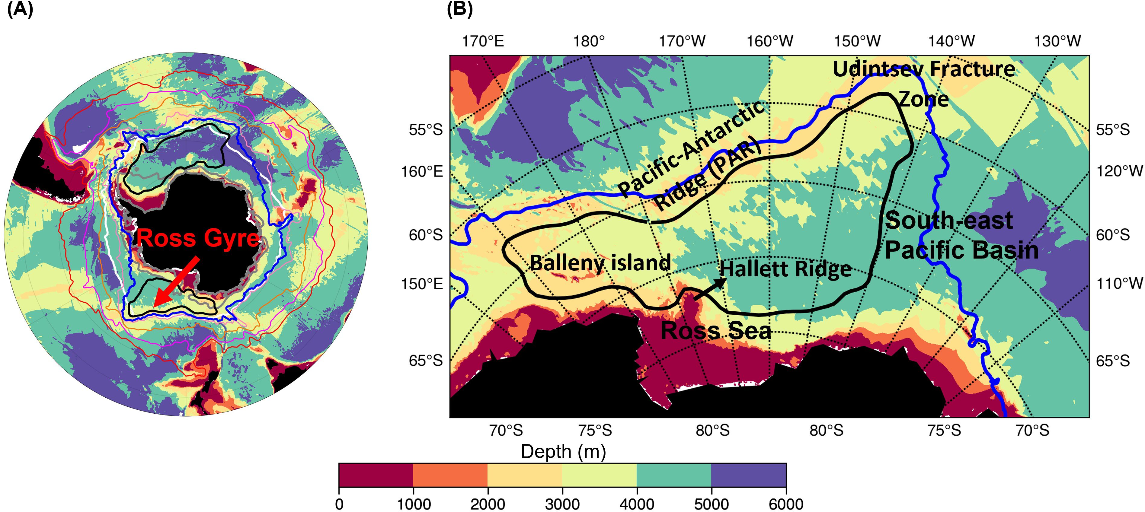
Figure 1. (A) Key climatological features of the Southern Ocean. The shadings are the bathymetry in meters and the colored contours correspond to the ACC boundaries and jets as described in Park et al. (2019). From north to south and in reddish colors are the northern boundary of the ACC (NBACC), the Subantarctic Front (SAF), the Polar Front (PF), and the Southern Antarctic Circumpolar Current Front (SACCF), respectively. The blue contour is the southern boundary of the ACC (SBACC). The black contours delineate the Weddell Gyre in the Atlantic Ocean and the Ross Gyre in the Pacific Ocean, based on recent satellite data (Armitage et al., 2018). The white and grey color contours are the sea-ice edges (ice concentration is 15%) for February and August, respectively. (B) Major topographic features in the Ross Gyre area (meters). The black contour is the Ross Gyre and the blue contour is the SBACC.

The ACC (Figure 1) consists of strong jets defined by fronts, i.e., the Sub-Antarctic Front (SAF), the Polar Front, and the Southern ACC Front, which are strongly steered by the topography. In between the southern boundary of the ACC (SBACC) and the Antarctic continental shelf break where the Antarctic Slope Current (ASC) encircles the Antarctic continent from east to west, lie the subpolar gyres. The subpolar gyres are covered by sea-ice almost fully during the austral winter and partially during the austral summer in the southern portion of the gyres. Both the relative warm interior water and the relatively cold water formed below the sea ice must pass through the intermediate current systems, i.e., the sub-polar gyres, in order to reach the marginal seas and the sub-Antarctic Ocean, respectively. There are two major subpolar gyres in the Southern Ocean. The first one, and the best documented, is the Weddell Gyre, located in the southern Atlantic Ocean (Gordon et al., 1981; Park and Gambéroni, 1995; Vernet and D., 2019) occupying the region between the Antarctic Peninsula and the Kerguelen Plateau. The second major subpolar gyre, located in the southwest Pacific, is the Ross Gyre (Dotto et al., 2018; Gouretski, 1999; Locarnini, 1994). A third subpolar gyre, the Australian–Antarctic Gyre (McCartney and Donohue, 2007; Aoki et al., 2010; Matsumura and Yamazaki, 2011), has been identified off East Antarctica.

The Ross Gyre (Figure 1) is a cyclonic circulation system located south of the ACC in the southwestern Pacific Ocean bounded by the Antarctic continent to the south. The Ross Sea, on the shelf, extends under the glacial ice front and is an important basin for the formation of the dense waters. The larger Ross Gyre system is constrained by major topographic features in the Pacific sector (Figure 1B). The Pacific-Antarctic Ridge (PAR), located in the northwestern part of the Ross Gyre, steers the ACC and separates the ACC from the gyre to the south. The Ross Gyre’s northern extremity is the Udintsev Fracture Zone where the ACC crosses the mid-ocean ridge (e.g. Park and Coauthors., 2019). The Ross Gyre recirculates water from the southern limits of the ACC across the deep expanse of the southeast Pacific Basin all the way to the continental slope. At the western limit of the Ross Gyre the Pacific-Antarctic Ridge merges with several ridge systems extending from the continent in the neighborhood of the Balleny Islands.

The southern portion of the Ross Gyre shows strong gradients in water mass properties, from Circumpolar Deep Water (CDW) to the Modified Circumpolar Deep Water (MCDW) to the Antarctic Surface Water (AASW; Jacobs, 1991; Rickard et al., 2010). Quantitative estimates of the gyre state are difficult to make from hydrographic observations alone due to the strong barotropic component of the circulation in this area of relatively weak stratification. Model representations of the subpolar gyres in the Southern Ocean exhibit large discrepancies (Wang and Meredith, 2008; Wang, 2013) and cannot be easily validated because of the lack of observations. Compared to the Weddell Gyre (see the review of Vernet et al., 2019), the Ross Gyre is less well observed though new techniques to exploit satellite data in sea-ice and under-ice Argo data are now providing much needed observations spanning the seasons in the subpolar regions of the Southern Ocean. While efforts have been made to describe the Ross Gyre using the various datasets, described below, the main drivers behind the Ross Gyre dynamics are not fully understood and have never been systematically examined.

Past research invokes a variety of forcing mechanisms for subpolar gyre circulation based on different indices or proxy quantities of circulation. Wang and Meredith (2008) found that the simulated sub-polar gyres strengths in the Southern Ocean in AR4 climate coupled models are more likely determined by upper layer meridional density gradients, which are determined predominantly by the salinity gradients, and the authors assert that the Sverdrup balance cannot be used to explain the modeled sub-polar gyres because the link between the gyre strengths and wind stress curl is weak. However, a more recent work by Armitage et al. (2018) show using novel data from radar altimetry that can measure the ice-covered sea surface height that the month-to-month circulation variability based on sea-surface height of the Ross and Weddell Gyres is strongly influenced by the local wind field and is correlated with the local wind curl. Dotto et al. (2018) also attributed the Ross Gyre’s variability to the Antarctic Oscillation (AO), a large-scale atmosphere mode and to the low sea-surface pressure of the Amundsen Sea Low mode. A recent idealized basin study argues that buoyancy forcing in a subpolar gyre is of similar importance to wind forcing and cannot be neglected (Hogg and Gayen, 2020), but the quantitative importance will depend on stratification, itself dependent on the buoyancy forcing.

The main objectives of this paper are a) to review the strength estimates of the Ross gyre using observations, reanalysis, and model simulations to provide a reference framework and b) to quantitatively estimate the contributions of the wind, buoyancy, eddies, and the ACC to the Ross Gyre circulation. The layout of the paper is as follows. In section 2, we use observations and existing reanalysis model simulations to review the latest gyre estimates. Next, in section 3, we introduce the regional HYCOM model configuration together with the vertically integrated vorticity equation that will be used to investigate the dynamical effects of various forcings on the Ross Gyre. We then present, in section 4, a series of sensitivity experiments designed to isolate the impact on the Ross Gyre circulation of a) the external forcings, i.e., the wind, and surface buoyancy, b) eddies, and c) the ACC. We then summarize and discuss our findings in the concluding section.

2 Ross Gyre extent and transport from observations and models

Before discussing the Ross Gyre’s extent, transport, and variability, it is important to define the gyre itself. One definition used by Dotto et al. (2018) is the largest possible closed contour of the dynamic ocean topography (DOT). The gyre center is then defined as the minimum DOT and the gyre transport is thus defined as the transport across the meridional section from the gyre center to the gyre southern boundary. Another way to characterize the gyre and gyre strength is to use the vertically integrated streamfunction with the gyre transport as the maximum streamfunction value. However, since observed velocities are not available, one has to make assumptions when applying the streamfunction-based definition to observational data from the Ross Gyre area. Dotto et al. (2018) used surface velocity throughout the water column to compute the transport, assuming no vertical shear. Another option is to estimate the vertical shear by applying the thermal wind relation to climatological T/S data.

The transport estimates of the Ross Gyre vary greatly in the literature, most likely due to disparities in the data sources, definitions of the gyre extent, and the methods used (see Table 1 for a review). Baroclinic estimates of the Ross Gyre transport are typically around 8 Sv by assuming no motion at the bottom (Gouretski, 1999). Reid (1986), Reid (1997), on the other hand, gives a transport closer to 20 Sv, because of an additional barotropic component based on observed westward bottom flows from a short current meter record. Chu and Fan (2007) suggest that the Ross Sea cyclonic gyre recirculates 15–30 Sv using an inverse model to calculate the volume transport from wind and hydrographic data. Models also show the gyre to be 20 Sv to 37 Sv, with large variations (Wang and Meredith, 2008; Mazloff et al., 2010; Rickard et al., 2010; Wang, 2013; Duan et al., 2016). A recent estimate of the Ross Gyre from altimetry data is about 23 Sv (Dotto et al., 2018) by, as noted above, assuming no vertical velocity shear in the interior ocean and computing the transport by multiplying the surface velocity with the ocean depth.

Table 1

Table 1. Ross Gyre Transport estimations.

We now re-examine the Ross Gyre extent and transport using the latest observational data and state-of-the-art model data. The Ross Gyre is depicted in Figure 2 from the perspective of DOT/Sea Surface Height (SSH) contours derived from observations and model outputs and its extent is defined as the largest closed DOT/SSH contour. The observed DOT datasets are obtained from two data sources: 1) the Armitage et al. (2018) archive, hereafter referred to as Armitage-2018, and 2) the Centre for Polar Observation and Modelling (CPOM, http://www.cpom.ucl.ac.uk/dynamic_topography/), hereafter referred to as CPOM-2021, which is similar to Armitage-2018, but with a different geoid (Armitage et al., 2016). Both datasets are on a 50 km grid with Armitage-2018 spanning 2011–2015, while CPOM-2021 spans from 2011-2019. Thus, the common period of 2011-2015 is chosen for the comparison. The SSH estimates of the ice-covered Southern Ocean are derived using radar altimetry data from the CyroSat-2 (CS-2) mission (Wingham et al., 2006) following the method by Kwok and Morison (2016) and combined with conventional open-ocean (ice-free) SSH estimates to produce monthly composites of DOT. Both datasets show the Ross Gyre spanning 160°E to 140°W, bounded by the Pacific-Antarctic Ridge in the northwest and the ACC to the east. The gyre exhibits little variability at the northern and southern boundaries, due to topographic constraints on the gyre (see Supplementary Figure S1). Larger variability exists at the eastern gyre boundary due to the variations of the position of the ACC. A smaller “sub-gyre” exists near the Balleny Islands to the west, as does a gyre extension into the Amundson Sea in the southeast. The climatological gyre center differs between the two datasets, with the gyre center near 67°S, 150°W in Armitage-2018 and 70°S, 165°W in CPOM-2021.

Figure 2

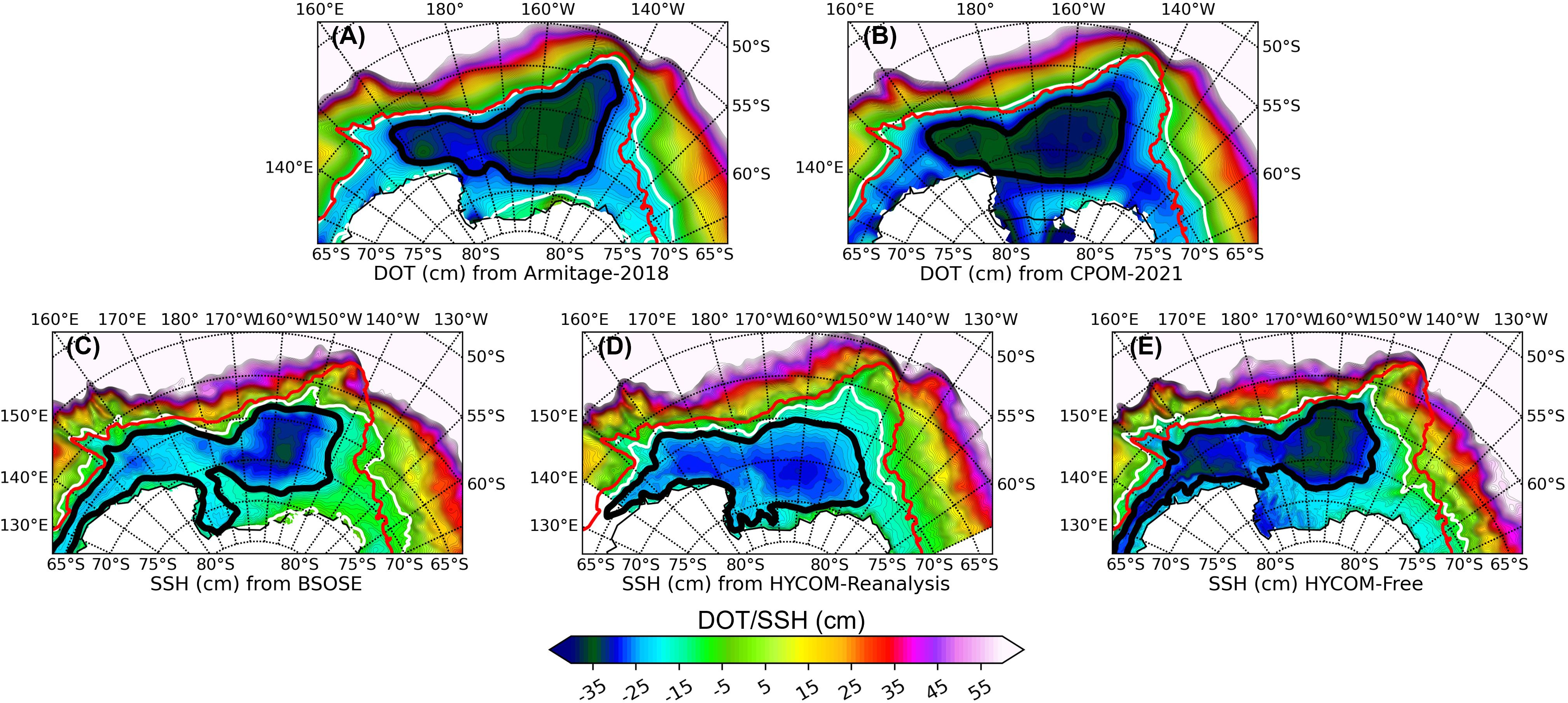
Figure 2. Extent of the Ross Gyre from observations (A, B) and models (C–E). In each figure, the shading is Dynamic Ocean Topography (DOT (cm), observation) or Sea Surface Height (SSH (cm), model) and domain average has been removed. The thick black contour is the climatological gyre boundary. The red contour is the southern boundary of the ACC defined in Park and Coauthors. (2019), while the white contour is the southern boundary of the ACC in each dataset. (A) is for Armitage-2018 data; (B) for CPOM-2021 data; (C) for B-SOSE; (D) for HYCOM-reanalysis; (E) for HYCOM-free.

Modelled SSH are from three sources: the Biogeochemical Southern Ocean State Estimate (B-SOSE) (Verdy and Mazloff, 2017); the global Hybrid Coordinate Ocean Model (HYCOM) (Bleck, 2002; Chassignet et al., 2003; Halliwell, 2004) reanalysis (Cummings and Smedstad, 2013); and a global HYCOM free simulation, i.e., without data assimilation (Chassignet et al., 2020). More details about the model setups can be found in Appendix A. The major difference between the modeled gyres and those derived from observations is that the modeled Ross Gyres usually extend farther west into the Southern Indian Ocean, even tending to form a so-called super gyre (Duan et al., 2016). The modeled gyre boundaries show less variability than in the observations, except for the HYCOM reanalysis which exhibits higher variability at the northern boundary (see Supplementary Figure S1) and where the whole gyre tends to shift to the south. The HYCOM free simulation provides a better gyre representation than the HYCOM reanalysis when compared to observations.

In the remainder of this section, we estimate and analyze the Ross Gyre transport using observations and the model output. Variables used to compute the estimates include DOT from observations, SSH from model output, temperature and salinity (T/S) from observations and model output, as well as velocities from Argo trajectories-based product and model output. Temperature is potential temperature unless otherwise specified. Details about the data can be found in Appendix A.

To get an estimate of the absolute or total Ross Gyre transport using the DOT, we need to derive 3D geostrophic velocities. The observed surface velocities are first calculated from the DOT using geostrophy. The subsurface absolute geostrophic velocities are then determined using the thermal wind relation from observational T/S data and the surface velocities (e.g., Kosempa and Chambers, 2014; Vigo et al., 2018). More details about these calculations can be found in Appendix B. The T/S data are from three climatological datasets [WOA18 (Boyer et al., 2018); GLODAPv2-2016b (Lauvset et al., 2016); and GDEM4 (Carnes et al., 2010)] that are widely used in the oceanography community and are considered best available estimates of the ocean state from observations on a large scale. Although these Ross gyre T/S datasets consist of climatological data, they do add a vertical shear contribution that one would not get if the surface velocity were assumed to extend all the way to the bottom (no vertical shear) as in Dotto et al. (2018). Once the full three-dimensional geostrophic velocities are available, the geostrophic vertically integrated streamfunction can be obtained by integrating the zonal absolute geostrophic velocity from the coast of Antarctica. To quantify how well this approximation works, we used the B-SOSE model to compare the transports computed using the full model velocities and those computed from three-dimensional geostrophic velocities. The two fields are almost identical (see Supplementary Figures S2, S3).

We apply the above transport calculation to the two observational monthly DOT data using the three available climatological T/S datasets mentioned earlier. The first set of results uses the Armitage-2018 DOT data, while the second uses the CPOM-2021 DOT data. The mean absolute geostrophic velocities, when compared at 1000 m depth to the mean velocities derived from ANDRO Argo floats displacement (Ollitrault and Rannou, 2013), are found to be in good agreement in terms of magnitude and pattern (see Supplementary Figures S4, S5 ). To compare quantitatively the results, we calculate the standard error between the calculated absolute geostrophic velocities with the velocities derived from the ANDRO Argo floats displacements, as summarized in Table 2. The combinations using GDEM4 T/S usually contain the largest errors, and errors of combinations using the Armitage-2018 DOT are smaller than those of combinations using CPOM-2021 DOT. The lowest errors in the zonal velocities are from the combination of Armitage-2018 DOT + WOA18 T/S, and the errors in the meridional velocities are also the lowest. The second and third lowest errors of the zonal velocities are from the combinations of Armitage-2018 DOT + GLODAPv2-2016b T/S and CPOM-2021 DOT + WOA18 T/S. Next, we will show how these three combinations better describe the gyre extent, with the Armitage-2018 DOT + GLODAPv2-2016b combination providing the most reasonable estimate.

Table 2

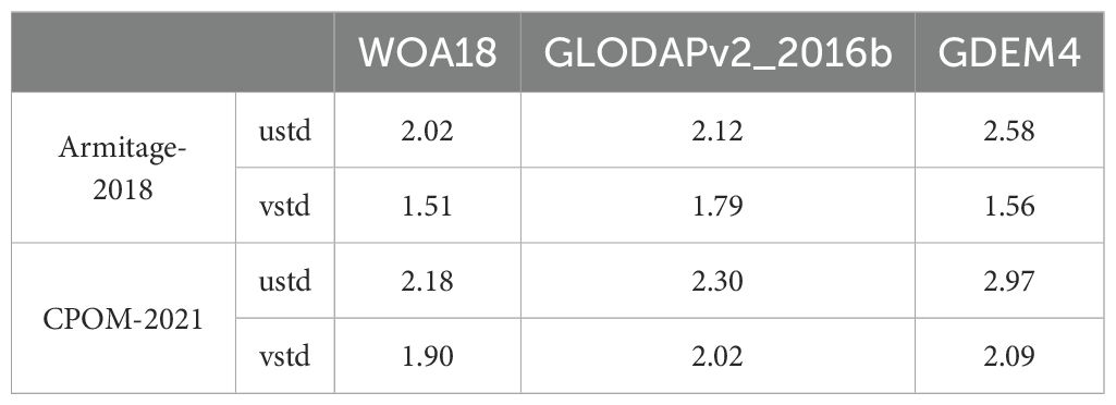
Table 2. Standard deviation (cm/s) of the difference between the geostrophic velocities with ANDRO velocities.

The next step is to define the gyre based on the geostrophic transport streamfunction. The gyre boundary is defined as the largest closed streamfunction contour, and the gyre center as where the maximum streamfunction is located in the domain. The Ross Gyre transport is defined as the zonal transport across the meridional section from the gyre center to the southern boundary. Two types of transport are defined: first, transport is computed from the 3D geostrophic velocities as described above; the second definition of transport assumes that there is no vertical shear and that the velocities are equal to the surface velocities as in Dotto et al. (2018). We define the first transport as the full transport, while the latter is referred to as the barotropic transport. Note that the term “barotropic” in “barotropic transport” here refers to vertical integration of velocities that are assumed to be equal the surface velocities (i.e., the velocity at the surface × depth) as in Dotto et al. (2018). Figure 3 shows the gyre extent from the geostrophic streamfunctions derived from the observations (Figures 3A–F), along with that from the streamfunctions for model outputs (Figures 3G–I). The mean gyre transports are summarized in Table 3. The result shows that there are large variations across the observational datasets, but this is the first time that large-scale subsurface velocities are used to perform Ross gyre transport calculations, providing more accurate observed transport estimates.

Figure 3

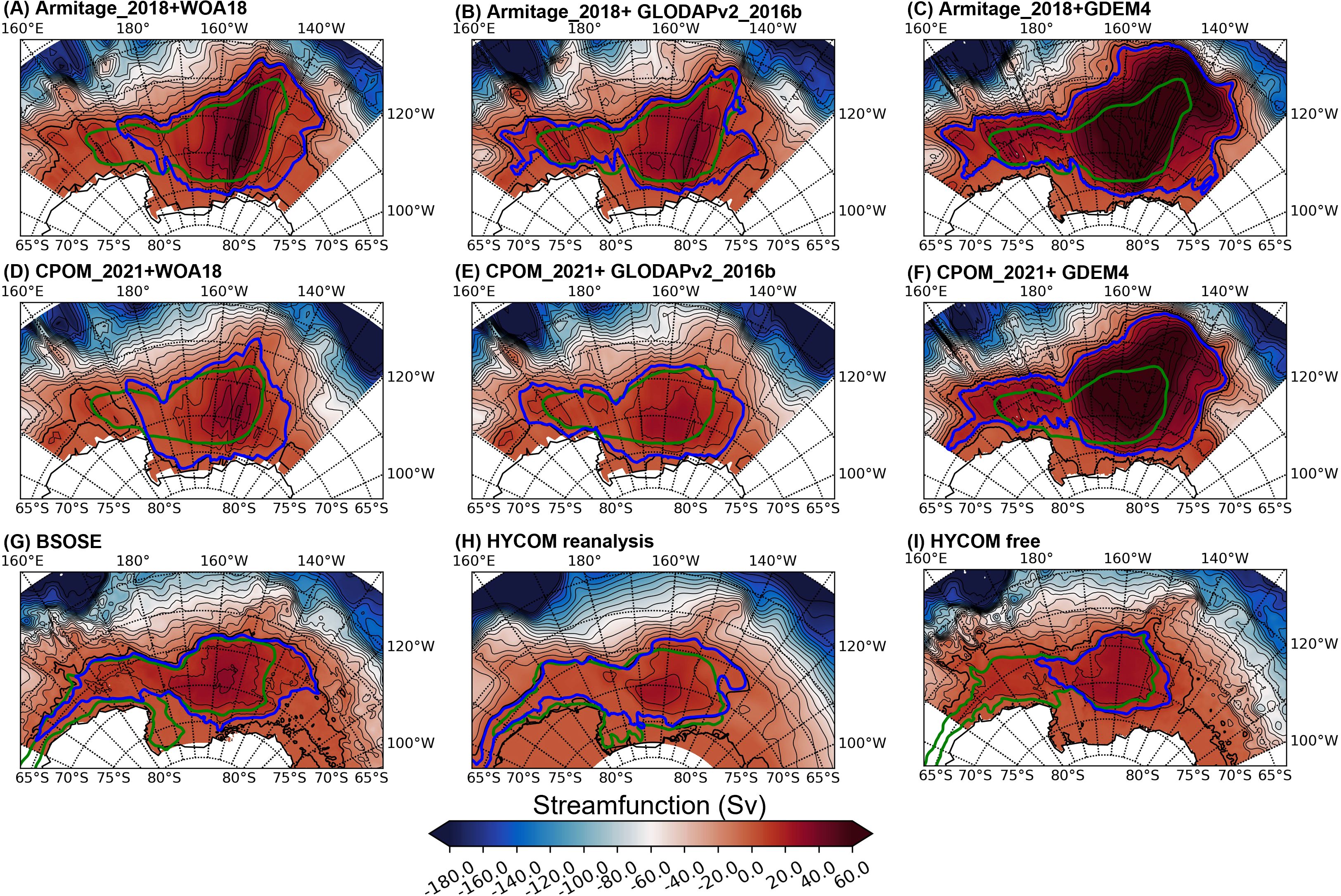
Figure 3. Climatological geostrophic streamfunctions (Sv) from observations and from models. (A–C) are for Armitage-2018) DOT + climatological T/S from WOA18, GLODAPv2-2016b and GDEM4 respectively; (D–F) are CPOM-2021 DOT + climatological T/S from WOA18, GLODAPv2-2016b and GDEM4 respectively; (G–I) are from B-SOSE, the HYCOM reanalysis, and the HYCOM free simulation, respectively. The black contours are in 10 Sv intervals, and the thick one is the 0 Sv contour. The overlayed colored contours (green and blue) are gyre extents identified either by largest extent of the closed contour of DOT/SSH (green) or streamfunction (blue), respectively.

Table 3

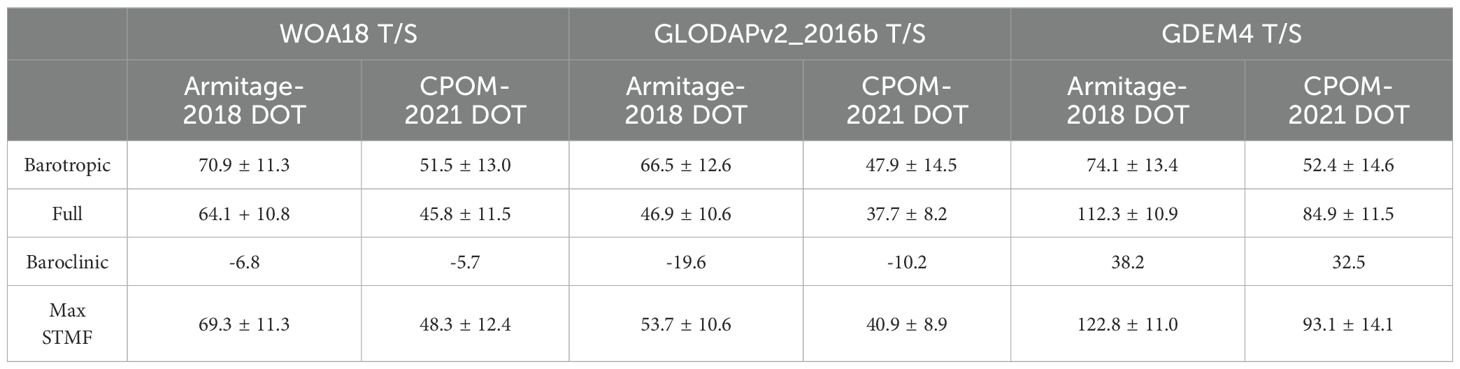
Table 3. Gyre transport (in Sv) from observations.

Considering the gyre extent, the streamfunction-based gyre boundaries are located more to the south and southeast than the DOT-based boundaries, incorporating the gyre extension into the Amundsen Sea. The GDEM4 combinations (Figures 3C, F), however, result in excessive gyre expansion into areas that are supposed to be part of the ACC from the DOT view, and the mean transport can exceed 110 Sv (Table 3). This is not too surprising since the GDEM4 combinations give large errors compared to the Argo-based observation. It is of particular interest to examine the details of the three observed combinations with lowest zonal velocity errors (Figures 3A, B, D, respectively). First, the gyres’ shapes follow the Pacific-Antarctic Ridge in the northwest very well, except for the Armitage-2018 + WOA18 combination which shows too much expansion into the ACC area. Second, the gyres extend into the Udintsev Fracture Zone, an important feature of the Ross Gyre. Third, the gyre boundaries in the southwest follow the shape of the Hallett Ridge, except for the CW combination. Additionally, the Armitage-2018 + GLODAPv2-2016b combination has a western extension of the Ross Gyre, which is often referred to as the Balleny Gyre, another important characteristic of the region.

The mean transport of the Armitage-2018 + WOA18, Armitage-2018 + GLODAPv2-2016b, and CPOM-2021 + WOA18 combinations are 64.1 + 10.8, 46.9 ± 10.6, and 45.8 ± 11.5 Sv, respectively (Table 3). These numbers are more than twice and even three times the typical value of ~20 Sv from several estimates (e.g. Reid, 1986 and Reid, 1997; Dotto et al., 2018), but closer to the 50 Sv transport anticipated by McCartney and Donohue (2007). The Armitage-2018 + GLODAPv2-2016b combination provides the best estimate of the Ross Gyre transport with lower zonal velocity errors, a good representation of the gyre extent, and a reasonable gyre transport estimate.

To evaluate the contributions of baroclinicity to the Ross Gyre strength, we also calculate the baroclinic transport (see Table 3) which is defined as the difference between the full transport and the barotropic transport which assumes that the velocity is uniform in vertical and equal to the surface velocity (i.e., the vertical integration of the surface geostrophic velocity × depth) (Dotto et al., 2018). The baroclinic transports of the WOA18 combinations are the smallest (-6.8 or -5.7 Sv, with the minus sign indicated a decrease in the transport) when compared to the others; the baroclinic contribution is of the opposite sign and too strong with GDEM4 (38.2 or 32.5 Sv) and moderate with GLODAPv2-2016b (-19.6 or -10.2 Sv).

Figure 4 shows the potential temperature, salinity, and zonal velocity along 150°W for the WOA18, GLODAPv2-2016b, and GDEM4 data. The potential densities (${\sigma }_2$) are plotted on top of the displayed variables (black contours). The zonal velocities are derived from the Armitage-2018 DOT and above T/S data. The climatological gyre center is typically around 150°W and 67°S. For the WOA18 data, due to the salinity maximum at depth of about 400-1500 m and south 69°S, the thermal wind accelerates the westward currents and decelerates the currents below. This means that, to some extent, the barotropic and baroclinic contributions cancel each other out during a vertical integration, and the overall impact of baroclinicity on the transport can be relatively small. For GDEM4, the continuous southward upward tilting of the density contour means an acceleration of the westward currents favors a stronger westward transport and can even reverse the velocity from eastward at the surface to westward in the subsurface. This will push the gyre center to the north of 65°S, and thus further facilitate a larger transport calculation. For GLODAPv2-2016b, the density contours tilt downward to the south over almost the entire depth, thus reducing the transport with a moderate impact on the full gyre transport.

Figure 4

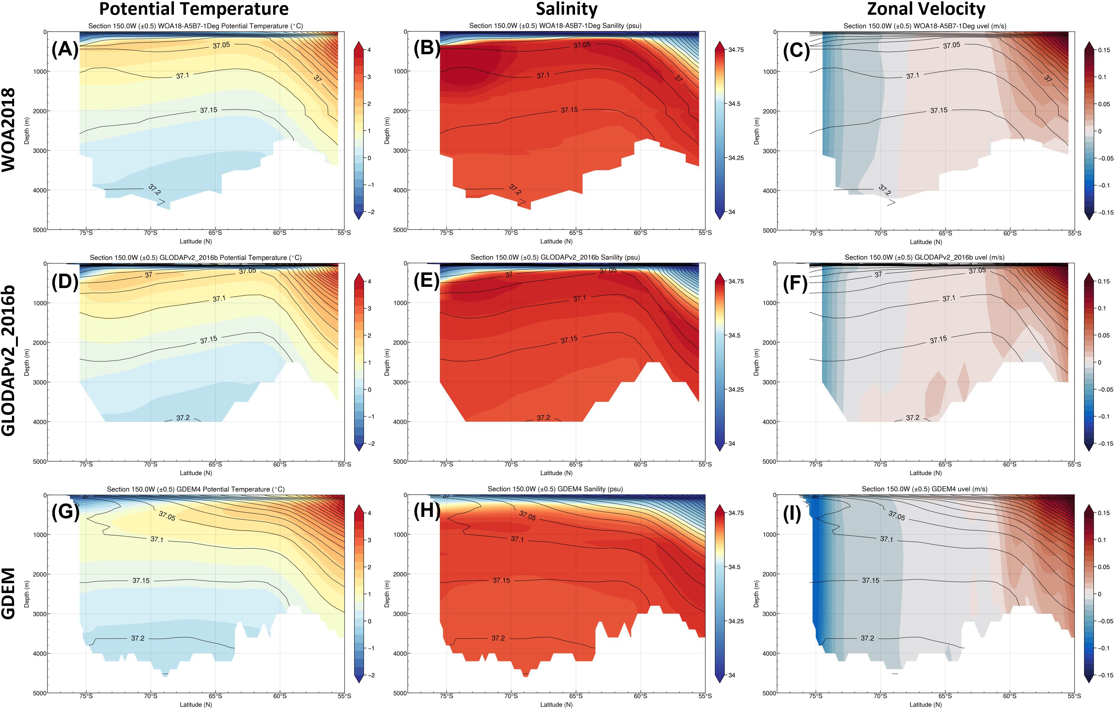
Figure 4. (A–C) are potential temperature (°C), salinity (psu), and zonal velocity (m/s) along 150°W for the WOA18 data; (D–F) are potential temperature, salinity, and zonal velocity along 150°W for the GLODAPv2-2016b data; (G–I) are potential temperature, salinity, and zonal velocity along 150°W for the GDEM4 data; The overlay contours are the potential density (kg/m³). The zonal velocities are based on the Armitage et al. (2018) DOT and corresponding T/S data.

Next, we discuss the time variability of the Ross Gyre from the observations. Three sets of indices are defined as proxies for the gyre variability: barotropic and full gyre transport along 150°W, and the maximum full streamfunction value. We focus mainly on the Armitage-2018 + GLODAPv2-2016b combination as it provides the best estimate of the Ross Gyre extent and transport. As it can be seen in Figure 5, the barotropic transport time series is significantly correlated (0.89) with that of the full transport. This is because the barotropic component dominates the full transport variability on monthly interannual time scales (Dotto et al., 2018). The maximum streamfunction time series are also highly correlated with the full transport time series. However, the transport south of the Ross Gyre, which contributes ~5 Sv to the maximum streamfunction, has little correlation with the gyre transport (-0.17), indicating that Antarctic Slope Current is not part of the southern branch of the Ross Gyre. Discussing the role of the Antarctic Slope Current is beyond the scope of this paper; nevertheless, the high correlations between the maximum streamfunction and the full transport indicate that it is adequate to use the maximum streamfunction to quantify the gyres’ variability. The gyre’s strength (defined as the full transport across the section from the gyre center to the gyre boundary) has been declining since 2012 (Figure 5B) and exhibits a strong seasonal cycle. It is usually strongest in the austral winter (peak in July), and weakest in austral summer (lowest in February), with two other sub-peaks in September and March. The barotropic and maximum streamfunction time series confirm these characteristics.

Figure 5

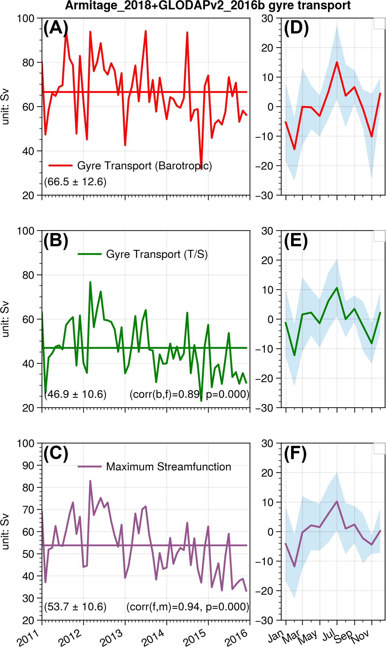
Figure 5. Gyre transport (Sv) time series based on the Armitage-2018 DOT and GLODAPv2-2016b T/S data: (A–F) are monthly transports and the corresponding annual cycle, respectively. The shadings in the annual cycle panels are the monthly standard deviation from the time series. The abbreviations b, f, and m in the correlations correspond to the barotropic transport, full gyre transport, and maximum streamfunction, respectively.

Because only annual mean climatological observed T/S data are available, we used the B-SOSE reanalysis data to quantify the impact of using climatological T/S when computing the transport. The comparison of the monthly SSH + mean T/S transport estimates to that of the monthly SSH + monthly T/S estimates shows that, by using monthly T/S, the correlations between the geostrophic transports and full model transports increase to 0.97, 0.95, and 0.58, respectively from 0.8, 0.63, and 0.38 when the mean T/S is used (as done with the observational data) for the maximum streamfunction, full and barotropic transport, respectively. This demonstrates that the computation is more accurate when the T/S data time variability is included and gives us confidence in the validity of the method used to estimate the transport of the Ross Gyre. Furthermore, the seasonal cycle is consistent across different scenarios (see Supplementary Figure S6), with the exception of the barotropic components because the B-SOSE model exhibits stronger baroclinicity, as described later.

The mean transport streamfunction from the numerical models are presented in Figures 3G–I along with the observations. The Ross gyre extents based on the streamfunction show better agreements than the SSH-based definition as in the observations. For example, the streamfunction-based gyre boundaries shift more to the south and to the southeast than the SSH-based boundaries, which includes the gyre extension into the Amundsen Sea. As summarized in Table 4, the models on average have a weaker gyre transport with less variability (see Supplementary Figure S7), with mean full transport of 30.5 ± 3.3 Sv, 18.2 ± 4.7 Sv, and 17.7 ± 3.9 Sv for B-SOSE, the HYCOM reanalysis, and the HYCOM free global simulation, respectively. The B-SOSE and the HYCOM free global simulations show strong baroclinic transport (-31.1 Sv and -20 Sv, respectively), which can be confirmed by looking at the T/S/U cross sections at 150°W (Figures 6A–C for B-SOSE and Figures 6G–I for the HYCOM free global simulation). The baroclinic transport can cancel about half of the barotropic transport (61.6 ± 9.2 Sv and 37.7 ± 7.0 Sv). Due to strong baroclinic transports, the correlations between barotropic transport and the full transport have lower values of 0.42 and 0.54 for B-SOSE and the HYCOM free global simulation, respectively. While the HYCOM reanalysis transport is more barotropic (24.0 ± 7.0 Sv), the baroclinic transport is only -5.8 Sv. Due to the weak baroclinicity (Figures 6D–F), the barotropic transports are highly correlated with the full gyre transport and the coefficient is 0.84. All the models illustrate that the maximum streamfunction is sufficient to represent the gyre variability due to their high correlation with the full gyre transport, with the coefficients of 0.91, 0.89, and 0.84 for B-SOSE, HYCOM reanalysis and HYCOM free global simulation.

Table 4

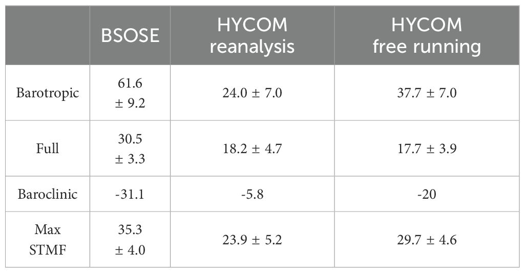
Table 4. Gyre transport (in Sv) from models.

Figure 6

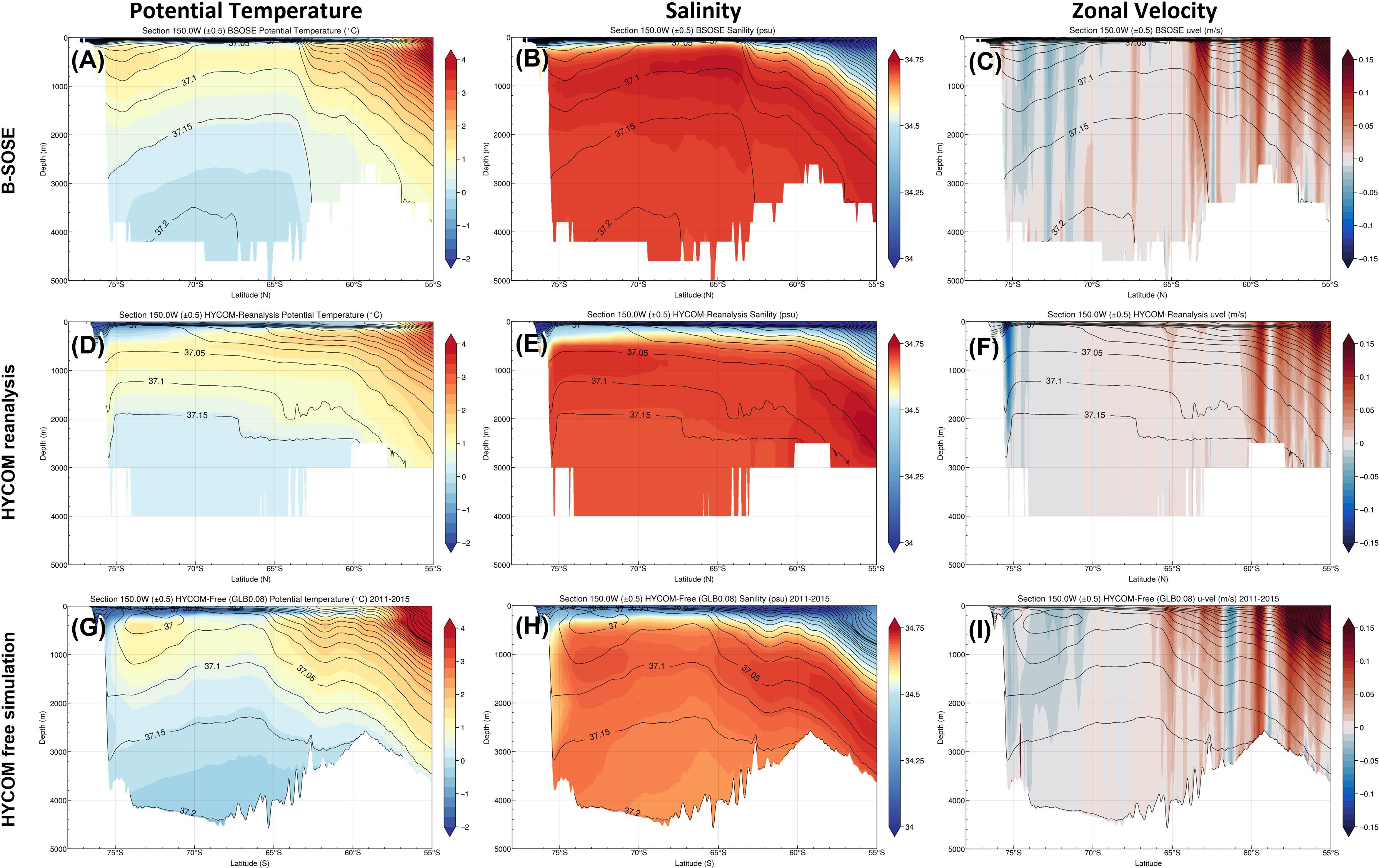
Figure 6. (A–C) are potential temperature (°C), salinity (psu), and zonal velocity (m/s) along 150°W for the B-SOSE data; (D–F) are potential temperature, salinity, and zonal velocity along 150°W for the HYCOM reanalysis data; (G–I) are potential temperature, salinity, and zonal velocity along 150°W for the HYCOM free global simulation data; the overlay contour and potential density (kg/m³). The zonal velocities are from direct model outputs.

3 Regional model configuration and vertically integrated vorticity analysis

3.1 Model configuration and experimental setup

The numerical model used for the regional experiments is HYCOM model which solves the hydrostatic primitive equations on its unique “hybrid” generalized vertical coordinate to combine the advantages of the different types of coordinates to optimally simulate coastal and open-ocean circulation features: in the open and stratified ocean, the isopycnic coordinate is primarily used in the interior to avoid spurious mixing arising from fixed vertical coordinates; the coordinate then smoothly transitions to z-level coordinates (levels at constant fixed depth or pressure) to maintain high vertical resolution in the surface mixed layer and sufficient vertical resolution in unstratified or weakly stratified regions of the ocean; and finally the coordinate becomes a terrain-following sigma coordinate in shallow coastal regions. The use of the generalized coordinate in HYCOM allows to adjust the vertical spacing of the coordinate surfaces and simplifies the numerical implementation of several physical processes (e.g., mixed layer detrainment, convective adjustment, sea ice modeling) (see Chassignet et al. (2006) for a review), while keeping an efficient vertical resolution throughout most of the ocean’s water column.

The surface atmospheric forcing data is from JRA55-do (version 1.4., Tsujino et al., 2018), used in phase 2 of OMIP for driving ocean-sea ice models. JRA55-do is based on the atmospheric reanalysis product JRA-55 (Kobayashi et al., 2015) with correction applied to it using satellite and other atmospheric reanalysis products. JRA55-do provides a high horizontal resolution (~55 km) and a temporal interval (3 h) that can suitably replace the current CORE/OMIP-1 dataset based on an assessment by Tsujino et al. (2020). Additional details can be found at (https://climate.mri-jma.go.jp/pub/ocean/JRA55-do/). The lateral boundary forcing is from the global 1/12° HYCOM global simulation without data assimilation (Chassignet et al., 2020). No ice components are calculated in the regional model, however the sea ice parameters (ice coverage, ice velocities, and surface heat and water fluxes) from the HYCOM global simulation are used as inputs to the regional model.

The horizontal resolution is 1/6° for the regional configuration (150E°-120°W – 78°S-57°S). The main reason we use 1/6° instead of 1/12° or higher is to match the 1/6° B-SOSE model resolution, and because of computational resource limitations. 1/6° is eddy-permitting in the Ross Gyre area. The regional model uses the same 36 hybrid coordinates of the 1/12° global HYCOM simulation in which it is nested. As shown in Figure 7, the gyre in the REFERENCE experiment can be clearly identified from the SSH contours (Figures 7A, B) and is similar to that of the HYCOM free global simulation used to force the regional model at the boundaries, although the gyre center is not as well defined. The full streamfunction map (Figures 7C, D) shows a stronger gyre transport in the regional model and is closer to observations. The thermal structure between the global model and the regional model are similar (see Supplementary Figure S8), which can be confirmed by the decomposition of the velocity into barotropic and baroclinic components (see Supplementary Figure S9). This difference is due to the barotropic response of the regional model to a stronger surface stress in the regional model (see Supplementary Figure S10) which arises from differences in the ice stress formulation between the two configurations (computed online versus prescribed).

Figure 7

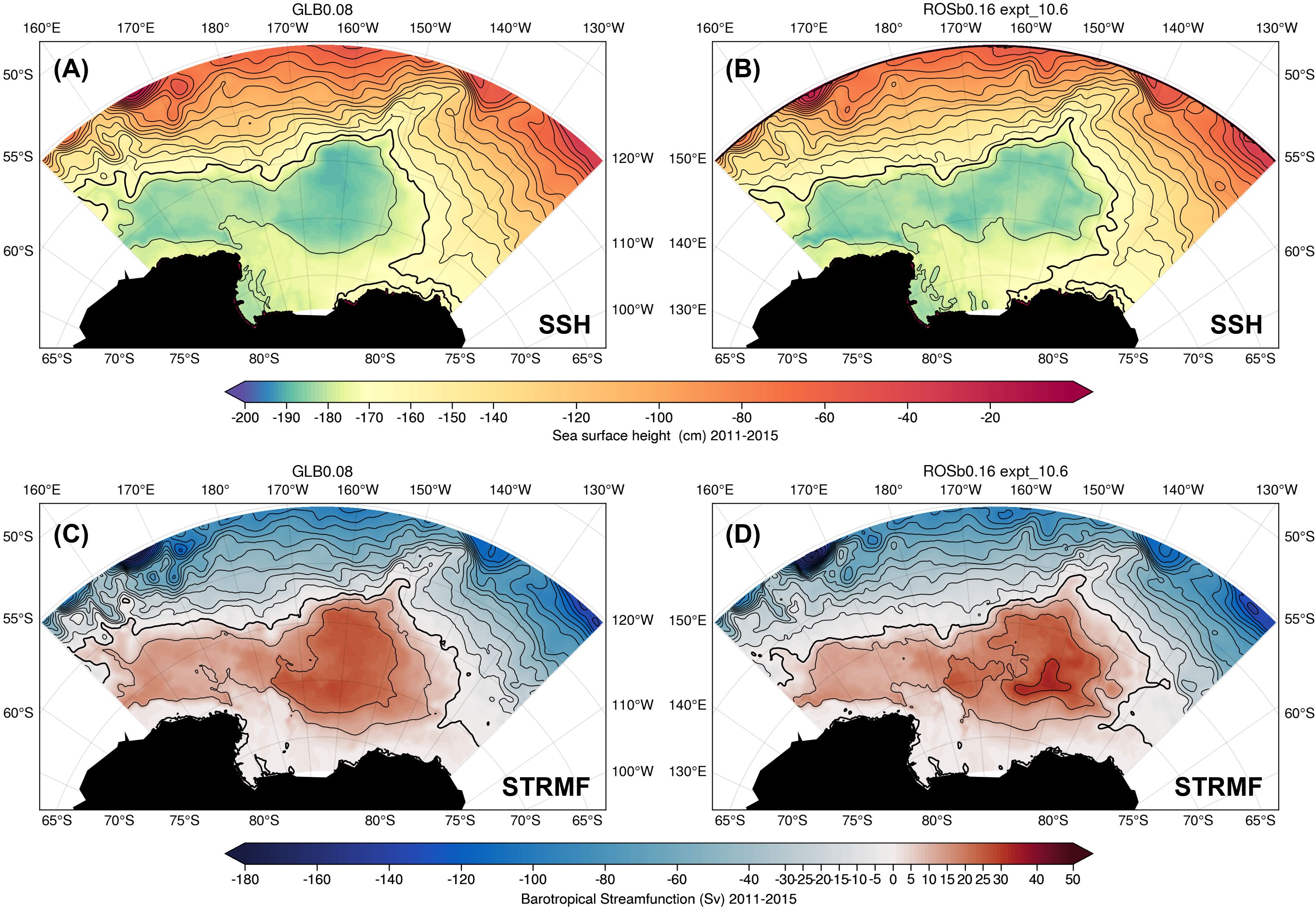
Figure 7. Global versus regional models: (A, C) are SSH (cm) and transport streamfunction (Sv) from the global simulation; (B, D) are from the regional model reference simulation.

3.2 Vertically integrated vorticity balance of the Ross Gyre

The aim of this section is to gain insight about the Ross Gyre dynamics by analyzing the vertically integrated vorticity balance in the regional REFERENCE configuration as well as in the B-SOSE ocean state estimate. A similar vorticity balance analysis has been used to study the dynamics of the subtropical and sub-polar gyres in the North Atlantic Ocean (e.g., Yeager, 2015; Schoonover et al., 2016; Alexander-Astiz Le Bras et al., 2019; Le Corre et al., 2020).

The vertically integrated vorticity equation is found by cross differentiating the vertically integrated momentum equation (Le Corre et al., 2020):

$$\begin{array}{c}\underset{\text{rate }}{\underbrace{\frac{\partial \omega }{\partial t}}}=\underset{\text{(a)}}{\underbrace{-\nabla \cdot (f\overline{\mathit{\text{u}}})}}+\underset{(b)}{\underbrace{\frac{J(P_b,h)}{{\rho }_0}}}+\underset{(c)}{\underbrace{\mathit{\text{k}}\cdot \nabla \times \frac{{\tau }_{\text{wind }}}{{\rho }_0}}}-\underset{(d)}{\underbrace{\mathit{\text{k}}\cdot \nabla \times \frac{{\tau }_{\text{bot }}}{{\rho }_0}}}+\underset{(e)}{\underbrace{A_{\text{Σ}}}}\hfill \\ +\underset{\text{(f) }}{\underbrace{N_{\text{Σ}}}}\hfill \end{array}$$

$\omega =k\cdot \nabla \times \overline{\mathit{\text{u}}}$ is the curl of the vertically integrated components of the velocity from the bottom to the surface where $\overline{\mathit{\text{u}}}=\underset{-h}{\overset{\eta }{\int }}\mathit{u}dz$ is the vertical integrated velocity, with $\mathit{u}=(u,v)$ the velocity in $(x,y)$, η the free surface height, and h the topography. The rate term on the left-hand side of the equation is negligible when averaged over a long time period. (a) is the planetary vorticity advection term, and for long enough time averaging period, $\nabla \cdot (f\overline{\mathit{\text{u}}})= -\beta \overline{v} -f\frac{\partial \eta }{\partial t}\approx -\beta \overline{v}$. We therefore define the planetary vorticity advection term as the β-term. (b) is the Jacobian of the bottom pressure and the depth, which is referred to as the bottom pressure torque (BPT) and includes the effect of the topography on the flow. This term can be written as $\frac{J(P_b,h)}{{\rho }_0}=f{\mathit{\text{u}}}_{gb}·\nabla h=f{w}_b$ when the geostrophic balance and the free-slip boundary condition are assumed, where ${\mathit{\text{u}}}_{gb}$ is the bottom geostropic velocity, and $w_b$ is the vertical velocity across the isobath. Therefore, the BPT represents the vortex stretching effects of the flow crossing isobaths. (c) is the wind stress curl of $k\cdot \nabla \times \frac{{\tau }_{\text{wind }}}{{\rho }_0}$, and (d) is $k\cdot \nabla \times \frac{{\tau }_{\text{bot }}}{{\rho }_0}$ and is the bottom drag curl (BDC). (e) is symbolized by $A_{\text{Σ}}$ and is the curl of the horizontal diffusion of momentum. BDC and $A_{\text{Σ}}$ may also be combined as the dissipation or friction torque term, as is done for the B-SOSE output. (f) $N_{\text{Σ}}$ is the nonlinear torque term arising from the advection terms in the momentum equation, which includes contributions from the curl of the vertically integrated momentum flux divergence, nonlinear vortex stretching, and vertical shear to barotropic vorticity transfer (Schoonover et al., 2016).

Figure 8 displays each of the vertically integrated vorticity equation components for the B-SOSE data. They have been smoothed with a Gaussian kernel of 1° to facilitate the interpretation. We can see that the BPT (Figure 8A) and nonlinear terms (Figure 8B) are balancing each other locally, and that the pattern of their summation (Figure 8F) matches the planetary vorticity advection term (β-term, Figure 8C). The surface stress curl (Figure 8D) is relatively weak when compared to the BTP and nonlinear terms. However, in the Ross Gyre, particularly in the interior, it is of the same order. The friction term (Figure 8E), i.e., the sum of horizontal viscosity and bottom drag, is very small, thus friction does not play a large role in the gyre vorticity balance in B-SOSE.

Figure 8

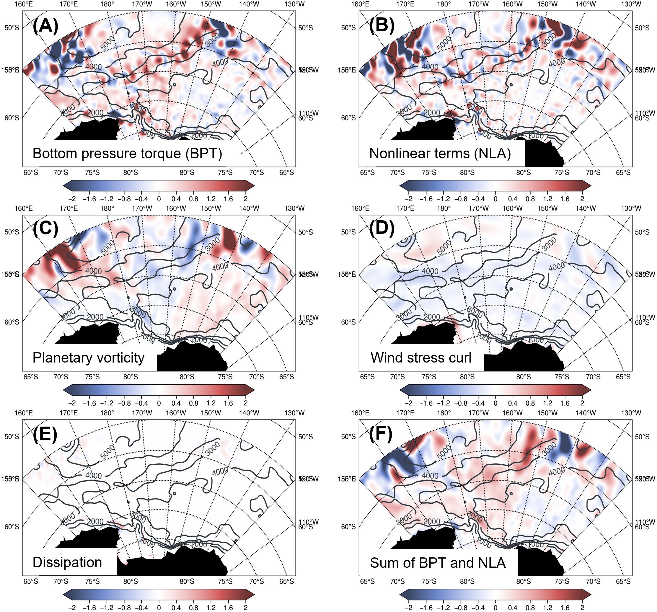
Figure 8. Spatial map of the time mean of each term in the vorticity equation in B-SOSE: (A) bottom pressure torque, (B) nonlinear terms, (C) the planetary vorticity, (D) wind stress curl, (E) and dissipation term. (F) sum of bottom pressure torque and non-linear terms. Unit for each term is m/s². The fields have been smoothed using a kernel of 1° radius. The black contours represent the bathymetry (m).

To see the effects of each term at the gyre scale, we perform spatial integrations to identify their contributions to the gyre (Figure 9). We use the largest possible closed contour of the full streamfunction to define the gyre. By integrating inside this contour, the major source of anti-cyclonic circulation of the gyre is the surface stress (Figure 9A), which is mainly balanced by the BPT term. The β-term is nearly zero since the closed stream function contour is selected. The nonlinear term contributes a small portion to the vorticity sources.

Figure 9

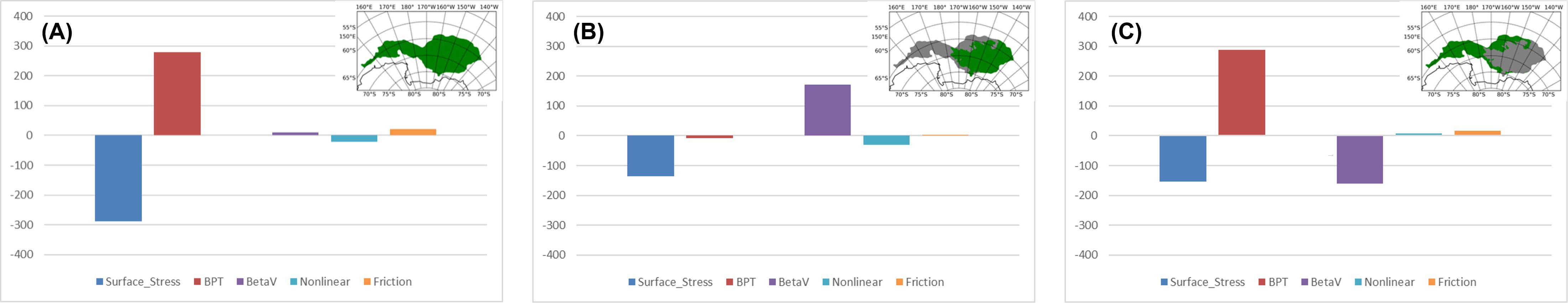
Figure 9. Area integral of each term of the vertically integrated vorticity equation in B-SOSE, (A) is for the whole gyre area by the largest closed streamfunction contour; (B, C) for gyre interior and boundary area. The unit is m³/s². The separation of interior and boundary is 4000 m model bathymetry.

Next, we divide the gyre into the interior and boundary domains. The area between the largest closed contour of the stream function and 4000 m is defined as the gyre boundary area (Figure 9C, the green shading), while the rest is the gyre interior (Figure 9B, the green shading). A depth of 4000 m is chosen because it roughly separates the relatively flat basin from the ridges in the west. The results are shown in Figure 9. In the gyre interior, the leading vorticity source term is the surface stress curl, which is in balance with the β-term. Other terms are small, indicating that the gyre interior is in the classical Sverdrup balance (Munk, 1950). Due to the weak stratification, the currents in the gyre boundary have strong barotropic components and are steered by the topography. The BPT term becomes the major vorticity sink term, the balance is between the surface stress curl, β-term, and the BPT. Thus, the gyre is in the so-called topographic Sverdrup balance (Le Corre et al., 2020) in the western boundary area, distinct from the classical Munk (1950) balance, in which the viscous effects were required to close the vorticity budget of the gyres.

The vertically integrated vorticity analysis (Figure 10) shows a similar dynamical regime in the HYCOM regional model to that of the B-SOSE model (Figure 9), in which the gyre is in the classical topographic Sverdrup/Sverdrup relation in the gyre boundaries/interiors. However, the BPT term is more important and becomes a major vorticity sink even larger than the β-term in the gyre interior, which modifies balance of the gyre interior toward the topographic Sverdrup balance and away from the standard Sverdrup balance. To document the impact of eddies, we decomposed the nonlinear term into the time mean and eddy terms (Figure 11). The nonlinear term as a whole is a weak vorticity source in the gyre interior and a sink in the gyre boundary area, and the eddy component is the major contributor to the nonlinear term.

Figure 10

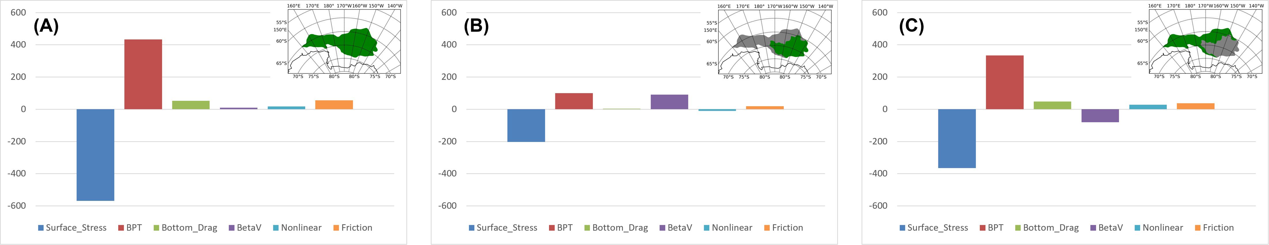
Figure 10. Area integral of each term of the vorticity equation for the regional HYCOM reference experiment, (A) is for the whole gyre area by the largest closed streamfunction contour; (B, C) for gyre interior and boundary area. The unit is m³/s². The separation of interior and boundary is 4000 m model bathymetry.

Figure 11

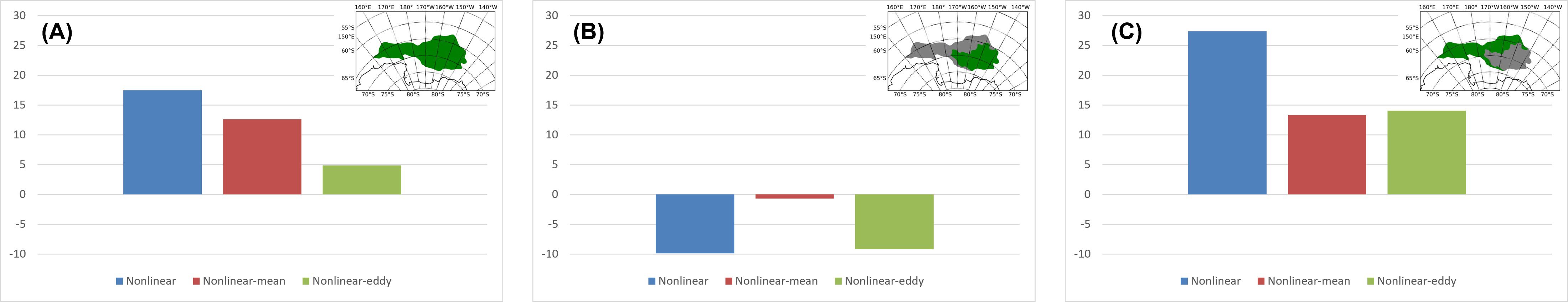
Figure 11. Area integral of nonlinear, nonlinear-mean and nonlinear-eddy for the regional HYCOM REFERENCE experiment, (A) is for the whole gyre area by the largest closed full streamfunction contour; (B, C) for gyre interior and boundary area. The unit is m³/s². The separation between the interior and boundary areas is the 4000 m model bathymetry.

Recent work has attributed the Ross Gyre variability to surface stress (e.g. Armitage et al., 2018; Dotto et al., 2018; Naveira Garabato et al., 2019; Auger et al., 2022). The vertically integrated vorticity analysis in our study also highlights the importance of the surface stress curl. The Ross Gyre is seasonally covered by sea-ice, thus the wind stress felt by the ocean is modulated by the sea ice. To demonstrate this situation, we decompose the stress felt by the ocean into the surface wind stress and ice stress. The surface stress can be formulated as in Tsamados et al. (2014):

$$\mathit{\text{τ}}=(1-\alpha ){\mathit{\text{τ}}}_{aw}+ \alpha {\mathit{\text{τ}}}_{iw}$$

where ${\mathit{\text{τ}}}_{aw}={\rho }_a{C}_d\left|{\mathit{\text{U}}}_{10}\right|{\mathit{\text{U}}}_{10}$is the wind stress, and ${\mathit{\text{τ}}}_{iw}={\rho }_w{C}_{diw}\left|{\mathit{\text{U}}}_i\right|{\mathit{\text{U}}}_i$ is the drag due to the movement of the sea ice. ${\mathit{\text{U}}}_{10}$ and ${\mathit{\text{U}}}_i$ are wind at 10m and ice velocity respectively. $\alpha$ is the sea ice concentration, ${\rho }_a=1.25 \text{kg}·{\text{m}}^{-3}$ is the air density, and $C_d$ is the air-ocean drag coefficient and set to be 1.25·10^-3. ${\rho }_w$ is the density of water and set to be 1026 kg·m^-3. $C_{diw}$ is the ice-water drag coefficient and we set it to be 0.00572, which is used in the HYCOM model by default.

Figure 12 shows the time series of average curls of wind stress (black), ice stress (blue) and surface stress (red) in the domain [160°W-130°W, 72°S-66°S] near the gyre center, along with the maximum geostrophic streamfunction (purple) from the combination of Armitage-2018 DOT + GLODAPv2-2016b T/S. The correlations between the maximum streamfunction, the wind stress curl, the ice stress curl, and the surface stress curl are (0.097, p= 0.462), (0.272, p= 0.036<0.05), and (0.31, p= 0.016<0.05), respectively. Thus, the ice stress and surface stress curl are significantly correlated with the maximum streamfunction, while the wind stress alone is not. The surface stress is dominated by the sea ice stress in winter and wind stress in summer. It is interesting to note the seasonal cycle of surface stress is similar to that of the maximum streamfunction, although there are some discrepancies.

Figure 12

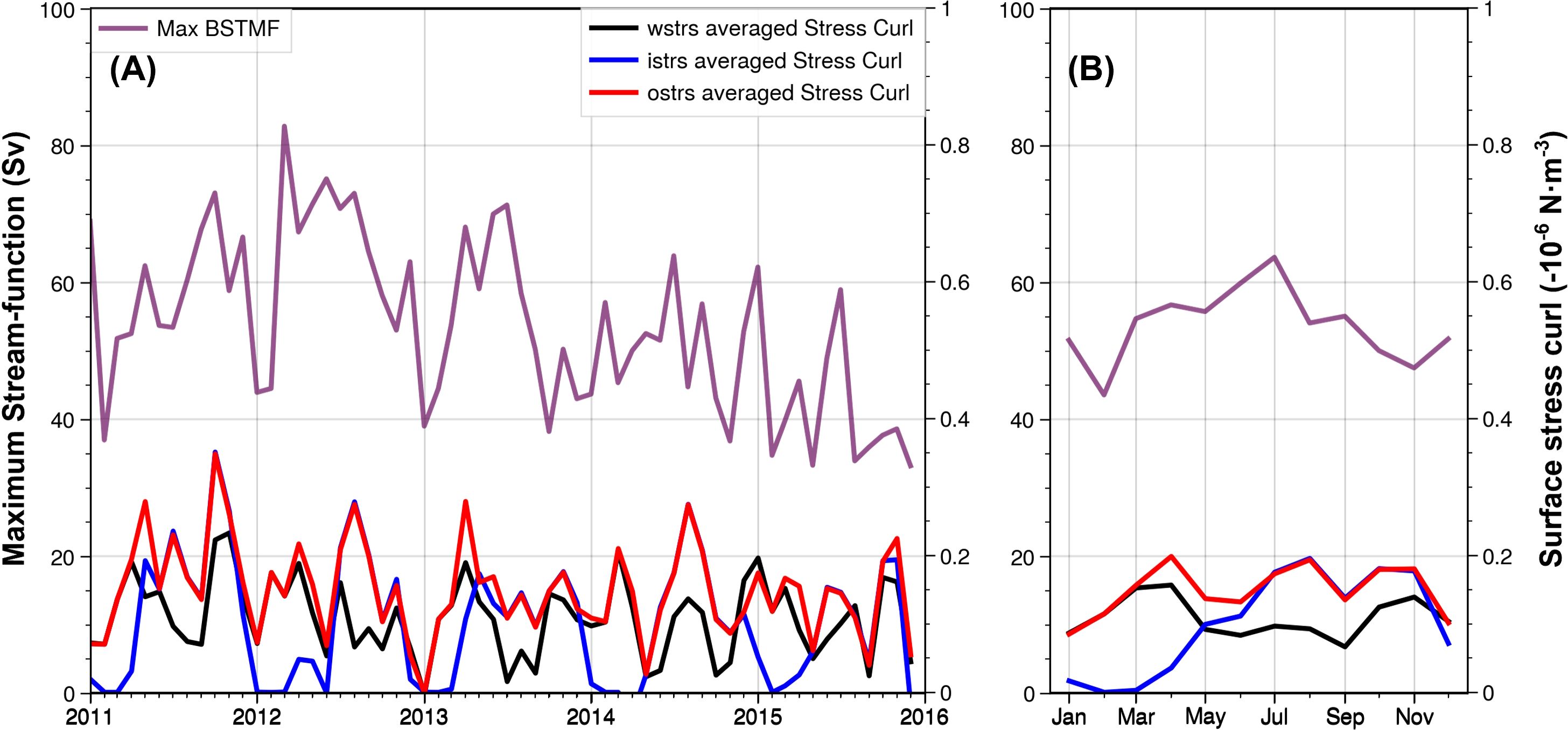
Figure 12. (A) Time series and (B) seasonal cycle of average curls of wind stress (black), ice stress (blue), and surface stress (red) in the domain of [160°W-130°W, 72°S-66°S], and the maximum geostrophic streamfunction (purple, Sv) from the combination of Armitage-2018 DOT + GLODAPv2-2016b T/S (AG combination). The unit for the stresses is N/m³.

The relation between the gyre variability and surface stress is much clearer in the regional model (Figure 13). The maximum streamfunction used here to represent the gyre variability is significantly correlated with averaged surface stress curl in the domain [160W°-130°W, 72°S-66°S] (coefficient is 0.77, p<0.001). There are two major peaks in the seasonal cycle of the streamfunction, one in August and the second one in October, both of which correspond to the maximums in wind stress curl. The gyre is usually weak in the austral summer when the sea ice is minimal, and the stress curl is the smallest. This significant correlation, together with the vertically integrated vorticity analysis results, is consistent with the surface stress being a key driver of the Ross Gyre.

Figure 13

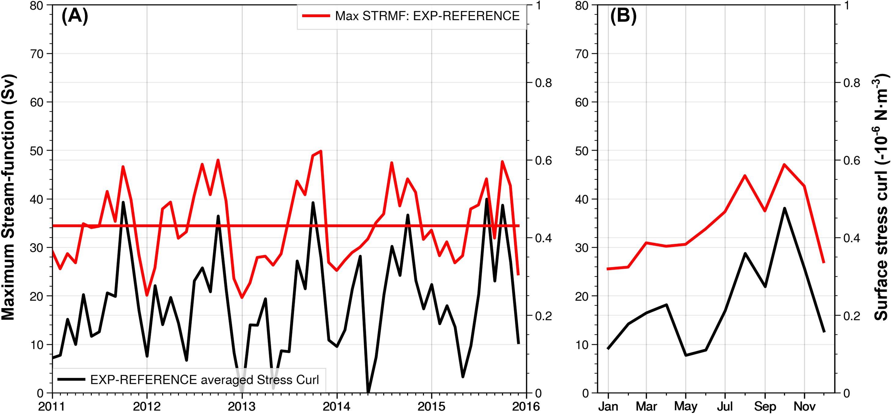
Figure 13. (A) Time series and (B) seasonal cycle of maximum streamfunction and average curls of wind stress in the regional HYCOM EXP-REFERENCE experiment. The red line is the maximum streamfunction (unit: Sv), while the black line is the average of the surface stress curls (unit: 10^-6 N·m^-3) in the domain [160°W-130°W, 72°S-66°S].

4 Sensitivity experiments

Several sensitivity experiments were performed to quantify the impact of a) the wind, b) buoyancy, c) non-linearity/eddies, and d) boundary conditions (see Table 5 for details). All regional sensitivity experiments are run for 11 years (2005-2015) with the analysis performed over the final five years.

Table 5

Table 5. Specifications of the numeric experiments.

4.1 Influence of surface stress

We have shown that the gyre variability is strongly correlated with the domain averaged surface wind stress curl. The vertically integrated vorticity analysis both in B-SOSE and the REFERENCE experiments also shows the gyre interior to be in the classic Sverdrup balance. It is therefore likely that the surface wind stress is a major driver of the Ross Gyre circulation and, to highlight this point, we performed the sensitivity experiment EXP-NO-STRESS by turning off all the surface wind stress induced forcing (including the ice stress). EXP-NO-STRESS exhibits a much weaker gyre than the REFERENCE experiment (Figure 14A), and the gyre retracts and decreases in strength by more than 25 Sv (Figure 14C). The center of the gyre also shifts to the southwest (Figure 14B). Due to the lack of upwelling induced by the surface stress, the interior isopycnic surfaces are flatter (see Supplementary Figure S11) hence the gyre is re-centered more to the south. Accordingly, the ACC without wind stress becomes broader, allowing more water intrusion from the north, and eventually bringing warmer and saltier water upward to the south. This weaker gyre, which we call the residual gyre (i.e., not wind driven), is therefore mostly driven by lateral boundary conditions i.e., the ACC, as discussed below. The seasonal cycle of the gyre also disappears (see Supplementary Figure S12).

Figure 14

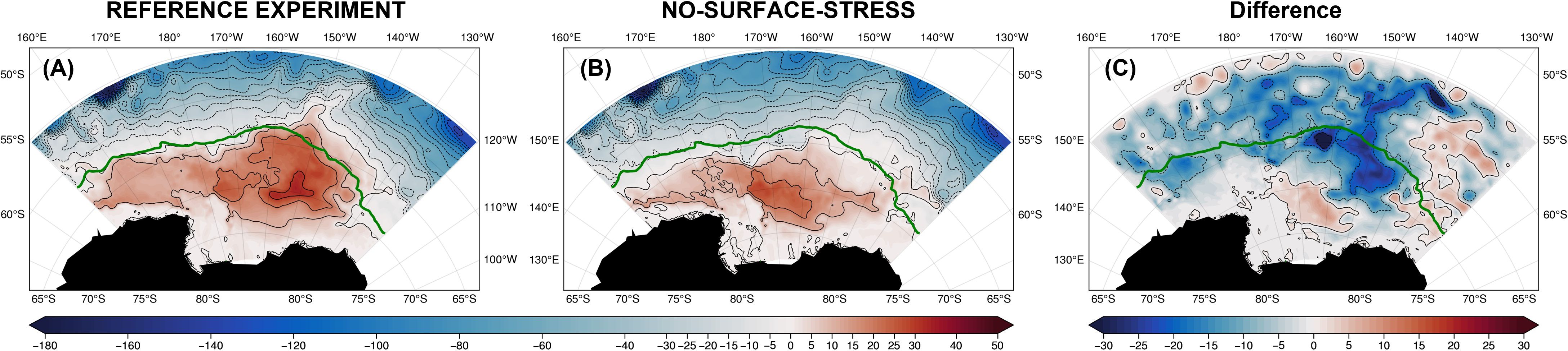
Figure 14. Streamfunction (Sv) for (A) the REFERENCE experiment; (B) EXP-NO-STRESS; and (C) their difference: (B) minus (A). The green line is the climatological edge of the maximum seasonal sea ice coverage.

4.2 Influence of non-linearity/eddies

The vorticity analysis also shows that the nonlinear term, which includes the effects of eddies, is not a major term from an integral balance perspective. However, it can be one of the largest terms locally. Further, we have shown that the eddy term dominates the nonlinear term. Thus, to examine the impact of eddies on the solution, we performed the experiment EXP-LINEAR by removing the nonlinear terms from the momentum model equations. As seen in Figure 15, in the absence of nonlinear terms, the downstream ACC becomes stronger, while the gyre extent is essentially the same as in the REFERENCE experiment; however, the northeastern part of the gyre shrinks and is bounded by a narrower jet. The mean gyre strength increases slightly (~2 Sv) and its variability is similar to that of the REFERENCE experiment (see Supplementary Figure S13). The vertically integrated vorticity analysis (see Supplementary Figure S14) for this experiment is very similar to the REFERENCE experiment, confirming that the nonlinear eddies are not an essential component on the gyre scale for our model configuration.

Figure 15

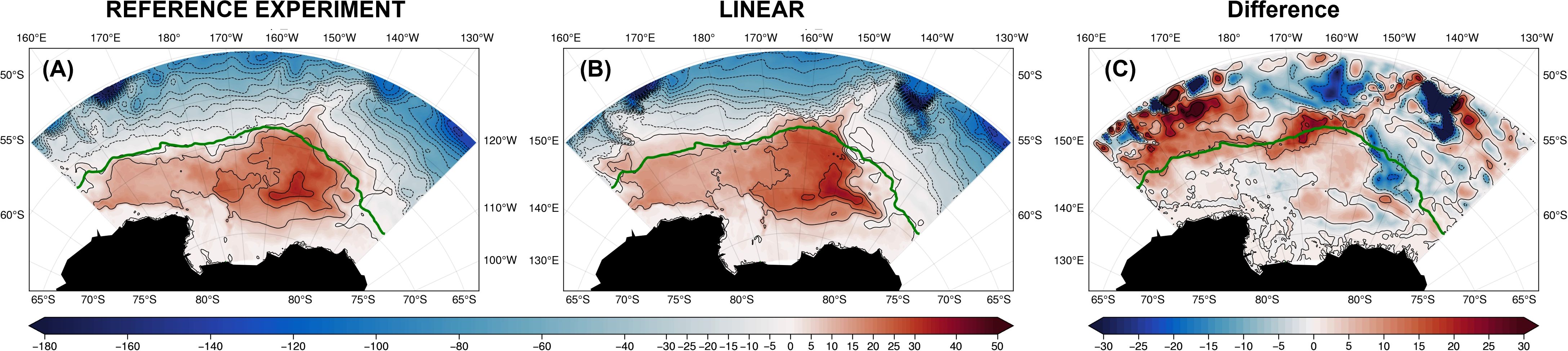
Figure 15. Streamfunction (Sv) for (A) the REFERENCE experiment; (B) EXP-LINEAR; and (C) their difference (B) minus (A). The green line is the climatological edge of the maximum seasonal sea ice coverage.

In Figure 16, one can however see that the slope of the isopycnal surfaces between the gyre and the ACC collapses in EXP-LINEAR resulting in flattened isopycnals, and that there is a strong T and S transition at the edge of sea ice coverage. Our EXP-LINEAR seems to imply that eddies may be responsible for maintaining the mean thermal structure; however, a linear model by necessity tends to shut off interior flow below the layer directly forced by the wind (Charney and Flierl, 1981). The presence of mean flow imposed by the boundary conditions implies that this effect does not apply in the ACC region. Outside this region topography hastens the shutdown, resulting in little vertical shear and relatively flat isopycnals. Furthermore, the stratification in the western part of the gyre is difficult to alter when the nonlinear terms are removed, possibly because the topography determines, to a large extent, the thermal or density structure, as surmised in the idealized modeling of Wilson et al. (2022).

Figure 16

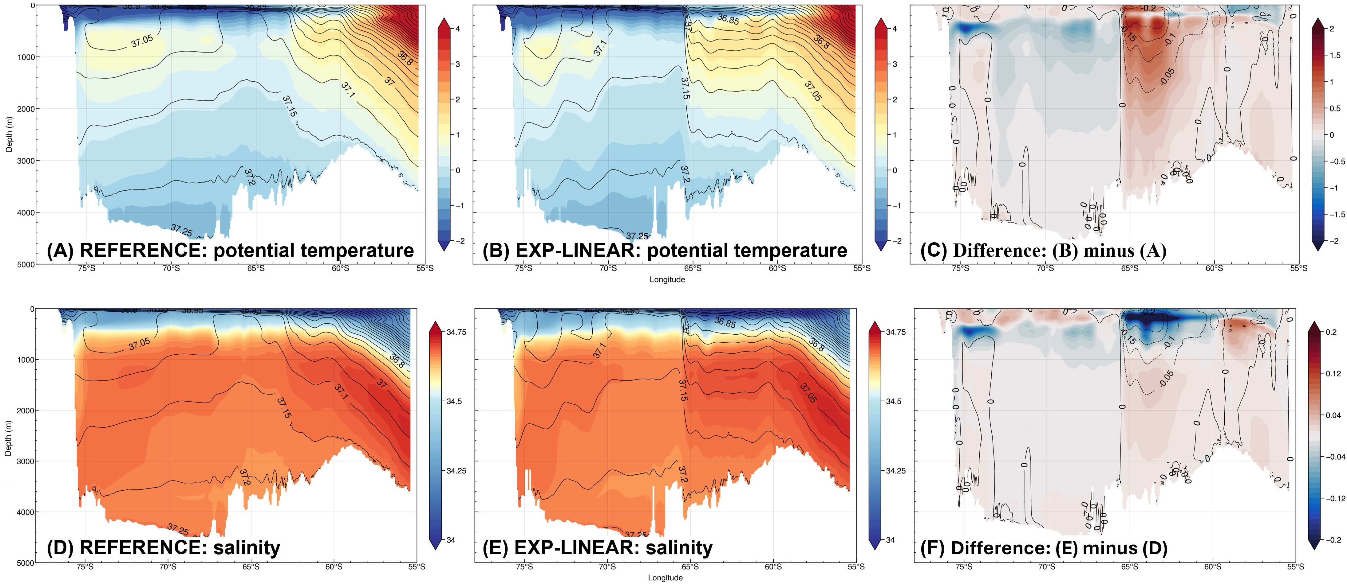
Figure 16. (A–C) are potential temperature (°C) along 150°W. (A) is the REFERENCE experiment, (B) is EXP-LINEAR, and (C) is their difference: (B) minus (A). (D–F) are salinity (psu) along 150°W. (D) is for the REFERENCE experiment, (E) is for EXP-LINEAR, and (F) is their difference: (E) minus (D). The overlay contours are potential density (A, B, D, E) or potential density difference (C, F).

4.3 Influence of surface buoyancy forcing

Surface buoyancy forcing is not explicitly quantified in the vertically integrated vorticity analysis, but we can explore its impact by removing it in the regional numerical experiment. The surface buoyancy forcing components are the heat flux, the E-P flux (evaporation - precipitation), and the salt flux due to the relaxation to sea surface salinity (SSS) used in the model. To turn off the surface buoyancy forcing, we set their values to zero everywhere. The resulting gyre is shown in Figure 17. The gyre transport in the Ross Sea area is weaker than in the REFERENCE experiment in the western part, while the northern part of the gyre center is stronger (~3 Sv). The gyre variability in transport shows little difference when compared to the REFERENCE experiment consistent with the gyre strength dominated by the surface stress.

Figure 17

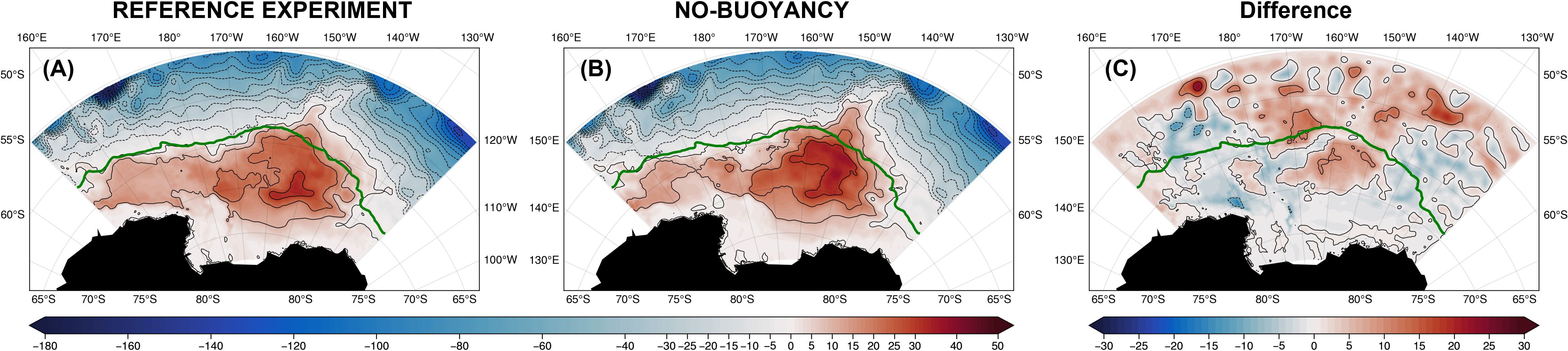
Figure 17. Streamfunction for (A) the REFERENCE experiment; (B) EXP-NO-BUOYANCY; and (C) their difference (B) minus (A). The green line is the climatological edge of the maximum seasonal sea ice coverage.

To further investigate the impact of the buoyancy forcing, we perform another experiment, EXP-NO-SURFACE-FORCING (Figure 18), where the surface buoyancy and wind forcing is turned off. This highlights the impact of the surface buoyancy in the absence of surface stress and helps us to identify if the surface buoyancy forcing can be responsible for the residual gyre (Figure 14B or Figure 18A) present when the surface wind stress is removed. Figure 18 shows that the surface buoyancy matters the most in the Ross Sea area where the dense water forms and contributes about 5-10 Sv to the residual gyre. Therefore, we conclude that the buoyancy forcing plays a local role in the Ross Sea where dense water is formed. It however cannot fully explain the presence of the residual gyre in the EXP-NO-STRESS (Figure 14B or Figure 18A).

Figure 18

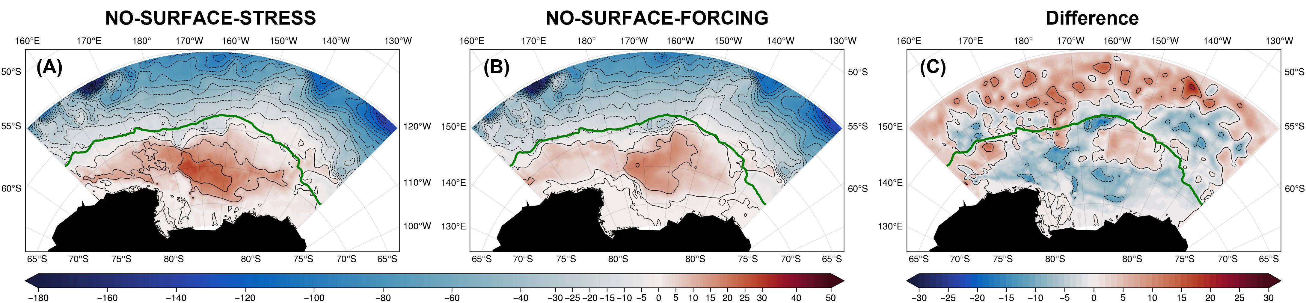
Figure 18. Streamfunction for (A) EXP-NO-STRESS; (B) EXP-NO-SURFACE-FORCING; and (C) their difference (B) minus (A). The green line is the climatological edge of the maximum seasonal sea ice coverage.

4.4 Influence of lateral boundary conditions

We demonstrated that surface stress is essential to the formation of the Ross Gyre in the EXP-NO-STRESS. A residual gyre however remains when the surface stress is turned off (Figure 14B or Figure 18A) and we have also shown that buoyancy forcing is not the primary factor driving the residual gyre in EXP-NO BUOYANCY: there is still a residual gyre after we turn off both the surface stress and buoyancy forcing in the EXP-NO-SURFACE-FORCING (Figure 18B). The only remaining factors that could force a residual gyre are either directly via the lateral boundary conditions prescribed at the open boundaries south of 62°S or indirectly by the ACC north of 62°S.

In both EXP-NO-STRESS, and EXP-NO-SURFACE FORCING, in addition to the ACC, one can notice that there is an inflow or outflow at the western boundary, south of the sea ice edge as indicated by the green line (15% sea ice concentration contour, Figure 19). To investigate whether the residual gyre is directly driven or not by the flow boundary conditions, we perform an experiment (EXP-NO-SURFACE-FORCING-WALL) identical to the EXP-NO-SURFACE-FORCING, except that we place a wall to the west boundary south of 62°S. The residual gyre in EXP-NO-SURFACE-FORCING-WALL (Figure 19B) is very similar to the gyre when the surface forcing is turned off (EXP-NO-SURFACE-FORCING) and we can clearly state that this residual gyre is not driven by the flows to the west of the gyre. It is therefore reasonable to conclude that this residual gyre must be indirectly driven by the ACC. This is consistent with Jayne et al. (1996) who used a quasi-geostrophic, homogeneous ocean model on β-plane and imposed a zonal jet at the western and eastern boundaries to mimic the ACC and showed that an inertial gyre can be driven by the instabilities of the ACC.

Figure 19

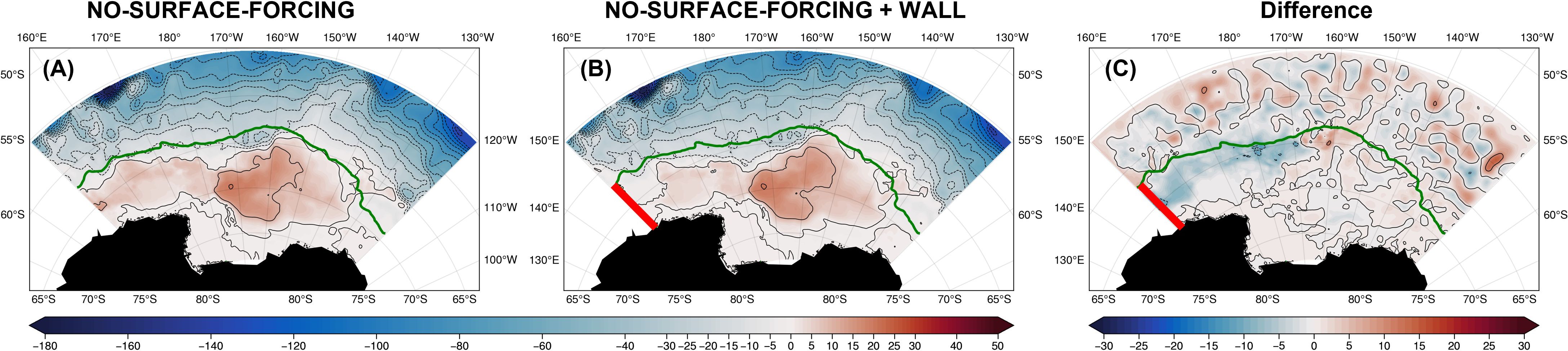
Figure 19. Streamfunction (Sv) for (A) the EXP-NO-SURFACE-FORCING experiment; (B) EXP-NO-SURFACE-FORCING-WALL; and (C) their difference (B) minus (A). The green line is the climatological edge of the maximum seasonal sea ice coverage. The bold red line on the west boundary of the domain south of 62ºS indicates the position where the relaxation to the lateral boundary is turning off to mimic a virtue wall.

5 Summary and discussion

Quantitative estimates of the Ross Gyre’s strength are difficult to obtain from hydrographic observations alone due to the limited sampling and the relatively weak stratification. As a result, one cannot fully evaluate the accuracy of the models, except over very limited areas. However, the latest available observational SSH data under the sea-ice provide new avenues to estimate the subsurface velocities with the aid of existing 3D climatological T/S data. The surface geostrophic velocities can be derived from the surface DOT data; then the subsurface absolute geostrophic velocities can be calculated using the thermal wind relation applied to the 3D climatological T/S data. Once the full 3D geostrophic velocities are available, the transport streamfunction was obtained by integrating the zonal velocity from the southern boundary and the Ross Gyre is defined by the largest closed transport streamfunction contour as the gyre boundary, with the gyre center defined as the maximum transport streamfunction in the gyre domain. The gyre transport is then the zonal transport of the meridional section from the gyre center to the gyre southern boundary. The mean transport of the Ross Gyre, based on our calculations, can be as much as 47 Sv, or twice the typical estimate of ~20 Sv. The Ross Gyre circulation does exhibit interannual transport variability and there is also a seasonal cycle, with the gyre strongest in the austral winter and weakest in the austral summer. The numerical models (reanalysis and free running) display weaker Ross Gyre transports due to a stronger baroclinic structure than that in the observations.

A vertically integrated vorticity analyses of the Ross Gyre show that it is primarily wind-driven in the interior and satisfies the classical Sverdrup balance (the balance between the wind stress curl and β-term). In the western boundary area of the gyre, the wind stress and the β-term are balanced by the bottom pressure torque, i.e., the topographic Sverdrup balance. This is distinct from the classical work of Munk (1950), in which the viscous effects were required to close the vorticity budget of the gyres. The nonlinear term, including contributions by eddies, does not appear to play a large role dynamically at the gyre scale, although it may dominate at local scales.

To estimate quantitatively the relative contributions of wind, buoyancy, eddies, and ACC on the Ross gyre circulation, regional sensitivity experiments to wind, buoyancy, nonlinearity, and boundary conditions were performed. The sensitivity experiments confirmed that the Ross Gyre, and its variability, is primarily wind-driven. Buoyancy forcing, nonlinear effects and eddies play a lesser role in the gyre dynamics. An important characteristic of the Ross Gyre is that it is covered by sea ice seasonally. The surface wind stress is controlled by the sea ice coverage, with a direct wind stress when there is no ice and stress from the ice dragging on the ocean surface when ice is present. Since the surface stress has been shown to be the main driver of the Ross Gyre circulation, it will be sensitive to the formulation of the stress from the sea ice (computed in real time or prescribed as in the regional experiments). A good representation of ice processes is therefore essential in simulating the Ross Gyre. Having an active ice model instead of a prescribed one would add another dimension that has not been considered here.

Topographic control of the subpolar gyres has been studied by Patmore et al. (2019) and Wilson et al. (2022). In Patmore et al. (2019), they found that a gyre can form without a continent boundary and tends to form along the eastern flank of a meridional ridge when it is steep enough. This finding is applicable to the Ross Gyre. In Wilson et al. (2022), the authors found that the zonally-oriented ridge along the northern edge of subpolar gyres plays a fundamental role in setting the weak stratification and well-confined gyre circulation. Their study focused on the Weddell Gyre, but their findings can be applied to the Ross Gyre because the Pacific-Antarctic Ridge provides a northern zonal oriented boundary to the Ross Gyre as well. The importance of the topography in setting the Ross Gyre circulation is highlighted by the vertically integrated vorticity analysis performed in this paper. The vorticity analysis shows the Ross Gyre satisfies two kind of Sverdrup balances. In the interior, the Ross Gyre is in the classic Sverdrup balance, i.e., the balance between the wind (surface) stress curl and the planetary vorticity advection or β-term. In the western gyre boundary area, the balance is the so-called topographic Sverdrup balance, in which the bottom pressure torque (BPT) becomes a major vorticity sink to balance the vorticity from wind stress and the β-term. It is not surprising that the BPT term is significant in this area. Due to the weak stratification, the circulation has a strong barotropic component, and thus can be strongly shaped by the topography around the gyre. This has also been shown to hold in the subpolar gyre in the North Atlantic (Hughes and de Cuevas, 2001; Spence et al., 2012; Yeager, 2015).

As indicated by Le Corre et al. (2020), studies that highlight the importance of the topographic Sverdrup balance are usually conducted on relatively coarse resolutions. Indeed, the horizontal resolution of the numerical outputs used in the vorticity analysis is only 1/6°, which is marginally eddy-resolving in the Ross Gyre area and we find that nonlinear terms do not play an essential role on the gyre scale in our analysis. However, locally, this nonlinear term can be important and is primarily balanced by the BPT as in Le Corre et al. (2020). In our numerical simulations, the nonlinear term plays a significant role in the northeastern part of the gyre and may play an essential role in maintaining the mean stratification there. Furthermore, the nonlinear term has been shown to be of importance in other regions of the world. Wang et al. (2017) showed the importance of nonlinear term in the dynamics the Gulf Stream recirculation gyres using high resolution (1/20°) simulations. By using a truly eddy-resolving (2 km) terrain-following coordinate model simulation, Le Corre et al. (2020) revisited the vorticity balance of the North Atlantic subpolar gyre and showed that the nonlinear term is a major cyclonic vorticity source that drives the subpolar gyre. Therefore, increasing the resolution of the regional model to truly resolve eddies in the Southern Ocean would be a natural extension of this study.

Data availability statement

The raw data supporting the conclusions of this article will be made available by the authors, without undue reservation.

Author contributions

YW: Conceptualization, Data curation, Formal analysis, Investigation, Methodology, Software, Validation, Visualization, Writing – original draft, Writing – review & editing. EC: Conceptualization, Formal analysis, Funding acquisition, Methodology, Project administration, Resources, Supervision, Validation, Writing – original draft, Writing – review & editing. KS: Conceptualization, Formal analysis, Methodology, Supervision, Validation, Writing – original draft, Writing – review & editing.

Funding

The authors declare financial support was received for the research, authorship, and/or publication of this article. This study was funded by the Office of Naval Research grant N00014-19-12674, by the National Aeronautics and Space Administration grant 80NSSC21K1500, and by the National Science Foundation grants OPP‐1643679 and OCE‐1658479.

Acknowledgments

YW extends his thanks to Dr. Matthew Mazloff for his help with the B-SOSE data.

Conflict of interest

The authors declare that the research was conducted in the absence of any commercial or financial relationships that could be construed as a potential conflict of interest.

Publisher’s note

All claims expressed in this article are solely those of the authors and do not necessarily represent those of their affiliated organizations, or those of the publisher, the editors and the reviewers. Any product that may be evaluated in this article, or claim that may be made by its manufacturer, is not guaranteed or endorsed by the publisher.

Supplementary material

The Supplementary Material for this article can be found online at: https://www.frontiersin.org/articles/10.3389/fmars.2024.1465808/full#supplementary-material

References

Alexander-Astiz Le Bras I., Sonnewald M., Toole J. M. (2019). A barotropic vorticity budget for the subtropical north atlantic based on observations. J. Phys. Oceanography 49, 2781–2797. doi: 10.1175/JPO-D-19-0111.1

Crossref Full Text | Google Scholar

Aoki S., Sasai Y., Sasaki H., Mitsudera H., Williams G. D. (2010). The cyclonic circulation in the Australian–Antarctic basin simulated by an eddy-resolving general circulation model. Ocean Dynamics 60, 743–757. doi: 10.1007/s10236-009-0261-y

Crossref Full Text | Google Scholar

Armitage T. W. K., Bacon S., Ridout A. L., Thomas S. F., Aksenov Y., Wingham D. J. (2016). Arctic sea surface height variability and change from satellite radar altimetry and GRACE 2003–2014. J. Geophysical Research: Oceans 121, 4303–4322. doi: 10.1002/2015JC011579

Crossref Full Text | Google Scholar

Armitage T. W. K., Kwok R., Thompson A. F., Cunningham G. (2018). Dynamic topography and sea level anomalies of the southern ocean: variability and teleconnections. J. Geophysical Research: Oceans 123, 613–630. doi: 10.1002/2017JC013534

Crossref Full Text | Google Scholar

Auger M., Sallée J.-B., Prandi P., Naveira Garabato A. C. (2022). Subpolar southern ocean seasonal variability of the geostrophic circulation from multi-mission satellite altimetry. J. Geophysical Research: Oceans. 127, e2021JC018096. doi: 10.1029/2021JC018096

Crossref Full Text | Google Scholar

Bleck R. (2002). An oceanic general circulation model framed in hybrid isopycnic-Cartesian coordinates. Ocean Model. 4, 55–88. doi: 10.1016/S1463-5003(01)00012-9

Crossref Full Text | Google Scholar

Boyer T. P., Baranova O. K., Coleman C., Garcia H. E., Grodsky A., Locarnini R. A., et al. (2018). World Ocean Database 2018. Mishonov A. Tech. Ed. (NOAA Atlas NESDIS), 87.

Google Scholar

Carnes M. R., Helber R. W., Barron C. N., Dastugue J. M. (2010). Validation test report for GDEM4. Memorandum report. Naval Research Laboratory Stennis Space Center, NRL/MR/7330--10-9271.

Google Scholar

Charney J. G., Flierl G. R. (1981) Evolution of physical oceanography: scientific surveys in honor of henry stommel. Eds. Warren B. A., Wunsch C. I. (M.I.T. Press, Cambridge, Massachusetts and London, England).

Google Scholar

Chassignet E. P., Hurlburt H. E., Smedstad O. M., Halliwell G. R., Wallcraft A. J., Metzger E. J., et al. (2006). Generalized vertical coordinates for eddy-resolving global and coastal ocean forecasts. Oceanography 19, 20–31. doi: 10.5670/oceanog

Crossref Full Text | Google Scholar

Chassignet E. P., Smith L. T., Halliwell G. R., Bleck R. (2003). North atlantic simulations with the hybrid coordinate ocean model (HYCOM): impact of the vertical coordinate choice, reference pressure, and thermobaricity. J. Phys. Oceanography 33, 2504–2526. doi: 10.1175/1520-0485(2003)033<2504:NASWTH>2.0.CO;2

Crossref Full Text | Google Scholar

Chassignet E. P., Yeager S. G., Fox-Kemper B., Bozec A., Castruccio F., Danabasoglu G., et al. (2020). Impact of horizontal resolution on global ocean–sea ice model simulations based on the experimental protocols of the Ocean Model Intercomparison Project phase 2 (OMIP-2). Geosci. Model. Dev. 13, 4595–4637. doi: 10.5194/gmd-13-4595-2020

Crossref Full Text | Google Scholar

Chu P. C., Fan C. (2007). An inverse model for calculation of global volume transport from wind and hydrographic data. J. Mar. Syst. 65, 376–399. doi: 10.1016/j.jmarsys.2005.06.010

Crossref Full Text | Google Scholar

Cummings J. A., Smedstad O. M. (2013). Variational Data Assimilation for the Global Ocean. In: Park S., Xu L. (eds). Data Assimilation for Atmospheric, Oceanic and Hydrologic Applications. (Vol. II). (Springer, Berlin, Heidelberg), 303–343. doi: 10.1007/978-3-642-35088-7_13

Crossref Full Text | Google Scholar

Cunningham S. A., Alderson S. G., King B. A., Brandon M. A. (2003). Transport and variability of the antarctic circumpolar current in drake passage. J. Geophysical Research: Oceans 108, 8084. doi: 10.1029/2001JC001147

Crossref Full Text | Google Scholar

Dotto T. S., Coauthors (2018). Variability of the ross gyre, southern ocean: drivers and responses revealed by satellite altimetry. Geophysical Res. Lett. 45, 6195–6204. doi: 10.1029/2018GL078607

Crossref Full Text | Google Scholar

Duan Y., Liu H., Yu W., Hou Y. (2016). The mean properties and variations of the Southern Hemisphere subpolar gyres estimated by Simple Ocean Data Assimilation (SODA) products. Acta Oceanologica Sin. 35, 8–13. doi: 10.1007/s13131-016-0901-2

Crossref Full Text | Google Scholar

Frölicher T. L., Sarmiento J. L., Paynter D. J., Dunne J. P., Krasting J. P., Winton M. (2015). Dominance of the southern ocean in anthropogenic carbon and heat uptake in CMIP5 models. J. Climate 28, 862–886. doi: 10.1175/JCLI-D-14-00117.1

Crossref Full Text | Google Scholar

Gordon A. L., Martinson D. G., Taylor H. W. (1981). The wind-driven circulation in the Weddell-Enderby Basin. Deep Sea Res. Part A. Oceanographic Res. Papers 28, 151–163. doi: 10.1016/0198-0149(81)90087-X

Crossref Full Text | Google Scholar

Gouretski V. (1999). The Large-Scale Thermohaline Structure of the Ross Gyre. In: Spezie G., Manzella G. M. R. eds. Oceanography of the Ross Sea Antarctica. (Springer, Milano), 77–100. doi: 10.1007/978-88-470-2250-8_6

Crossref Full Text | Google Scholar

Halliwell G. R. (2004). Evaluation of vertical coordinate and vertical mixing algorithms in the HYbrid-Coordinate Ocean Model (HYCOM). Ocean Model. 7, 285–322. doi: 10.1016/j.ocemod.2003.10.002

Crossref Full Text | Google Scholar

Hogg A. M. (2010). An Antarctic Circumpolar Current driven by surface buoyancy forcing. Geophysical Res. Lett. 37, e2020GL088539. doi: 10.1029/2020GL088539

Crossref Full Text | Google Scholar

Hogg A. M., Gayen B. (2020). Ocean gyres driven by surface buoyancy forcing. Geophysical Res. Lett. 47, e2020GL088539. doi: 10.1029/2020GL088539

Crossref Full Text | Google Scholar

Hughes C. W., de Cuevas B. A. (2001). Why western boundary currents in realistic oceans are inviscid: A link between form stress and bottom pressure torques. J. Phys. Oceanography 31, 2871–2885. doi: 10.1175/1520-0485(2001)031<2871:WWBCIR>2.0.CO;2

Crossref Full Text | Google Scholar

Hunke E., Lipscomb W. (2010). CICE: The Los Alamos sea ice model documentation and software user's manual version 4.1. Los Alamos, NM, Los Alamos National Laboratory. Tech. Rep. LA-CC-06-012. 76 pp.

Google Scholar

Jacobs S. S. (1991). On the nature and significance of the Antarctic Slope Front. Mar. Chem. 35, 9–24. doi: 10.1016/S0304-4203(09)90005-6

Crossref Full Text | Google Scholar

Jayne S. R., Hogg N. G., Malanotte-Rizzoli P. (1996). Recirculation gyres forced by a Beta-plane jet. J Phys Oceanogr. 26, 492–504.

Google Scholar

Kobayashi S., Coauthors (2015). The JRA-55 reanalysis: general specifications and basic characteristics. J. Meteorological Soc. Japan. Ser. II 93, 5–48. doi: 10.2151/jmsj.2015-001

Crossref Full Text | Google Scholar

Kosempa M., Chambers D. P. (2014). Southern Ocean velocity and geostrophic transport fields estimated by combining Jason altimetry and Argo data. J. Geophysical Research: Oceans 119, 4761–4776. doi: 10.1002/2014JC009853

Crossref Full Text | Google Scholar

Kwok R., Morison J. (2016). Sea surface height and dynamic topography of the ice-covered oceans from CryoSat-2: 2011–2014. J. Geophysical Research: Oceans 121, 674–692. doi: 10.1002/2015JC011357

Crossref Full Text | Google Scholar

Lauvset S. K., Coauthors (2016). : A new global interior ocean mapped climatology: the 1° × 1° GLODAP version 2. Earth Syst. Sci. Data 8, 325–340. doi: 10.5194/essd-8-325-2016

Crossref Full Text | Google Scholar

Le Corre M., Gula J., Tréguier A. M. (2020). Barotropic vorticity balance of the North Atlantic subpolar gyre in an eddy-resolving model. Ocean Sci. 16, 451–468. doi: 10.5194/os-16-451-2020

Crossref Full Text | Google Scholar

Locarnini R. A. (1994). Water masses and circulation in the Ross Gyre and environs (Office of Graduate Studies: Texas A&M University).

Google Scholar

Marshall J., Adcroft A., Hill C., Perelman L., Heisey C. (1997). A finite-volume, incompressible Navier Stokes model for studies of the ocean on parallel computers. J. Geophysical Research: Oceans 102, 5753–5766. doi: 10.1029/96JC02775

Crossref Full Text | Google Scholar

Marshall J., Radko T. (2003). Residual-mean solutions for the antarctic circumpolar current and its associated overturning circulation. J. Phys. Oceanography 33, 2341–2354. doi: 10.1175/1520-0485(2003)033<2341:RSFTAC>2.0.CO;2

Crossref Full Text | Google Scholar

Marshall J., Speer K. (2012). Closure of the meridional overturning circulation through Southern Ocean upwelling. Nat. Geosci 5, 171–180. doi: 10.1038/ngeo1391

Crossref Full Text | Google Scholar

Matsumura S., Yamazaki K. (2011). Eurasian subarctic summer climate in response to anomalous snow cover. J. Climate 25, 1305–1317. doi: 10.1175/2011JCLI4116.1

Crossref Full Text | Google Scholar

Mazloff M. R., Heimbach P., Wunsch C. (2010). An eddy-permitting southern ocean state estimate. J. Phys. Oceanography 40, 880–899. doi: 10.1175/2009JPO4236.1

Crossref Full Text | Google Scholar

McCartney M. S., Donohue K. A. (2007). A deep cyclonic gyre in the Australian–Antarctic Basin. Prog. Oceanography 75, 675–750. doi: 10.1016/j.pocean.2007.02.008

Crossref Full Text | Google Scholar

Meier W. N., Fetterer F., Savoie M., Mallory S., Duerr R., Stroeve J. (2017). NOAA/NSIDC Climate data record of passive microwave sea ice concentration, version 3. Boulder, Colorado USA: NSIDC: National Snow and Ice Data Center. doi: 10.7265/N59P2ZTG

Crossref Full Text | Google Scholar

Munk W. H. (1950). On the wind-driven ocean circulation. J. Meteor 7, 79–93. doi: 10.1175/1520-0469(1950)007<0080:OTWDOC>2.0.CO;2

Crossref Full Text | Google Scholar

Naveira Garabato A. C., Coauthors (2019). Phased response of the subpolar southern ocean to changes in circumpolar winds. Geophysical Res. Lett. 46, 6024–6033. doi: 10.1029/2019GL082850

Crossref Full Text | Google Scholar

Ollitrault M., Rannou J. P. (2013). ANDRO: an argo-based deep displacement dataset. J. Atmospheric Oceanic Technol. 30, 759–788. doi: 10.1175/JTECH-D-12-00073.1

Crossref Full Text | Google Scholar

Orsi A. H., Whitworth T., Nowlin W. D. (1995). On the meridional extent and fronts of the Antarctic Circumpolar Current. Deep Sea Res. Part I: Oceanographic Res. Papers. 42, 641–673. doi: 10.1016/0967-0637(95)00021-W

Crossref Full Text | Google Scholar

Park Y. H., Park T., Kim T.-W., Lee S.-H., Hong C.-S., Lee J.-H., et al. (2019). Observations of the antarctic circumpolar current over the udintsev fracture zone, the narrowest choke point in the southern ocean. J. Geophysical Research: Oceans 124, 4511–4528. doi: 10.1029/2019JC015024

Crossref Full Text | Google Scholar

Park Y. H., Gambéroni L. (1995). Large-scale circulation and its variability in the south Indian Ocean from TOPEX/POSEIDON altimetry. J. Geophysical Research: Oceans 100, 24911–24929. doi: 10.1029/95JC01962

Crossref Full Text | Google Scholar

Patmore R. D., Holland P. R., Munday D. R., Garabato A. C. N., Stevens D. P., Meredith M. P. (2019). Topographic control of southern ocean gyres and the antarctic circumpolar current: A barotropic perspective. J. Phys. Oceanography 49, 3221–3244. doi: 10.1175/JPO-D-19-0083.1

Crossref Full Text | Google Scholar

Reid J. L. (1986). On the total geostrophic circulation of the South Pacific Ocean: Flow patterns, tracers and transports. Prog. Oceanography 16, 1–61. doi: 10.1016/0079-6611(86)90036-4

Crossref Full Text | Google Scholar

Reid J. L. (1997). On the total geostrophic circulation of the pacific ocean: flow patterns, tracers, and transports. Prog. Oceanography 39, 263–352. doi: 10.1016/S0079-6611(97)00012-8

Crossref Full Text | Google Scholar

Rickard G. J., Roberts M. J., Williams M. J. M., Dunn A., Smith M. H. (2010). Mean circulation and hydrography in the Ross Sea sector, Southern Ocean: representation in numerical models. Antarctic Sci. 22, 533–558. doi: 10.1017/S0954102010000246

Crossref Full Text | Google Scholar

Rintoul S. R. (2018). The global influence of localized dynamics in the Southern Ocean. Nature 558, 209–218. doi: 10.1038/s41586-018-0182-3

PubMed Abstract | Crossref Full Text | Google Scholar

Rintoul S. R., Garabato A. C. N. (2013). Dynamics of the Southern Ocean circulation. Siedler G., Griffies S., Gould J., Church J. (eds.) Ocean Circulation and Climate: A 21st Century Perspective, 2nd Ed. (Oxford, GB: Academic Press), pp. 471–492.

Google Scholar

Schoonover J., Dewar W., Wienders N., Gula J., McWilliams J. C., Molemaker M. J., et al (2016). North atlantic barotropic vorticity balances in numerical models. J. Phys. Oceanograp. 46, 289–303. doi: 10.1175/JPO-D-15-0133.1

Crossref Full Text | Google Scholar

Spence P., Saenko O. A., Sijp W., England M. (2012). The role of bottom pressure torques on the interior pathways of north atlantic deep water. J. Phys. Oceanography 42, 110–125. doi: 10.1175/2011JPO4584.1

Crossref Full Text | Google Scholar

Tsamados M., et al (2014). Impact of variable atmospheric and oceanic form drag on simulations of arctic sea ice. J. Phys. Oceanography 44, 1329–1353. doi: 10.1175/JPO-D-13-0215.1

Crossref Full Text | Google Scholar

Tschudi M., Meier W. N., Stewart J. S., Fowler C., Maslanik J. (2019). Polar Pathfinder Daily 25 km EASE-Grid Sea Ice Motion Vectors, Version 4. Boulder, Colorado USA: NASA National Snow and Ice Data Center Distributed Active Archive Center. doi: 10.5067/INAWUWO7QH7B

Crossref Full Text | Google Scholar

Tsujino H., Urakawa H., Nakano R. J., Small W. M., Kim S. G., Yeager G., et al (2018). : JRA-55 based surface dataset for driving ocean–sea-ice models (JRA55-do). Ocean Model. 130, 79–139. doi: 10.1016/j.ocemod.2018.07.002

Crossref Full Text | Google Scholar

Tsujino H., Urakawa S. M., Griffies G., Danabasoglu A. J., Adcroft A. E., Amaral T., et al (202). : Evaluation of global ocean–sea-ice model simulations based on the experimental protocols of the Ocean Model Intercomparison Project phase 2 (OMIP-2). Geosci. Model. Dev. 13, 3643–3708. doi: 10.5194/gmd-13-3643-2020

Crossref Full Text | Google Scholar

Verdy A., Mazloff M. R. (2017). A data assimilating model for estimating Southern Ocean biogeochemistry. J. Geophysical Research: Oceans 122, 6968–6988. doi: 10.1002/2016JC012650

Crossref Full Text | Google Scholar

Vernet M., Coauthors (2019). The weddell gyre, southern ocean: present knowledge and future challenges. Rev. Geophysics 57, 623–708. doi: 10.1029/2018RG000604

Crossref Full Text | Google Scholar

Vigo M. I., García-García D., Sempere M. D., Chao B. F. (2018). 3D geostrophy and volume transport in the southern ocean. Remote Sens. 10, 715. doi: 10.3390/rs10050715

Crossref Full Text | Google Scholar

Wang Y., Claus M., Greatbatch R., Sheng J. (2017). Decomposition of the Mean Barotropic Transport in a High-Resolution Model of the North Atlantic Ocean: North Atlantic Barotropic Transport. Geophys. Res. Lett. 44, 11,537–11,546. doi: 10.1002/2017GL074825

Crossref Full Text | Google Scholar

Wang Z. (2013). On the response of Southern Hemisphere subpolar gyres to climate change in coupled climate models. J. Geophysical Research: Oceans 118, 1070–1086. doi: 10.1002/jgrc.20111

Crossref Full Text | Google Scholar

Wang Z., Meredith M. P. (2008). Density-driven Southern Hemisphere subpolar gyres in coupled climate models. Geophysical Res. Lett. 35, L14608. doi: 10.1029/2008GL034344

Crossref Full Text | Google Scholar

Wilson E. A., Thompson A. F., Stewart A. L., Sun S. (2022). Bathymetric control of subpolar gyres and the overturning circulation in the southern ocean. J. Phys. Oceanography 52, 205–223. doi: 10.1175/JPO-D-21-0136.1

Crossref Full Text | Google Scholar

Wingham D. J., Coauthors (2006). CryoSat: A mission to determine the fluctuations in Earth’s land and marine ice fields. Adv. Space Res. 37, 841–871. doi: 10.1016/j.asr.2005.07.027

Crossref Full Text | Google Scholar

Yeager S. (2015). Topographic coupling of the atlantic overturning and gyre circulations. J. Phys. Oceanography 45, 1258–1284. doi: 10.1175/JPO-D-14-0100.1

Crossref Full Text | Google Scholar

Appendix A: Data description

The DOT are obtained from two data sources: Armitage et al. (2018), hereafter referred to as Armitage-2018, and the Centre for Polar Observation and Modelling, University College London (CPOM, http://www.cpom.ucl.ac.uk/dynamic_topography/), hereafter referred to as CPOM-2021, which is the same as Armitage-2018, but uses a different geoid (Armitage et al., 2016). The former is on a 50 km grid spanning 2011–2015, while the latter is also 50 km, but spans from 2011-2019. Thus, the common period from 2011-2015 is chosen for comparison. The SSH estimates of the ice-covered Southern Ocean are derived using radar altimetry data from the CyroSat-2 (CS-2) mission (Wingham et al., 2006) following the method by Kwok and Morison (2016) and combined with conventional open-ocean (ice-free) SSH estimates to produce monthly composites of DOT.

Observational T/S data originate from three climatological datasets: WOA18 (Boyer et al., 2018), GLODAPv2-2016b (Lauvset et al., 2016), and GDEM4 (Carnes et al., 2010). These datasets are widely used in the oceanography community and are considered the best available estimates of the ocean state from observations on a large scale. However, they are only available as annual climatology.

Model datasets include: the Biogeochemical Southern Ocean State Estimate (B-SOSE) (Verdy and Mazloff, 2017); the global Hybrid Coordinate Ocean Model (HYCOM) (Bleck, 2002; Chassignet et al., 2003; Halliwell, 2004) reanalysis (Cummings and Smedstad, 2013); and a global HYCOM free simulation, i.e., without data assimilation (Chassignet et al., 2020).

SOSE (Mazloff et al., 2010) is a physically realistic estimate product of the Southern Ocean state. It is achieved be by constraining the MIT General Circulation Model (MITgcm) (Marshall et al., 1997) by least squares fit to all available observations of the ocean, which is accomplished iteratively through an adjoint method. The B-SOSE, a coupled biogeochemical-sea ice-ocean state estimate, is the latest SOSE product. It has a horizontal resolution of 1/6° and 52 vertical layers with thickness ranges from 4.6 m near the surface to 400 m near the bottom. More data descriptions can be found on the SOSE website (http://sose.ucsd.edu/sose.html).

The HYCOM reanalysis, short for HYCOM+NCODA (Navy Coupled Ocean Data Assimilation) Ocean Reanalysis, has a 1/12° horizontal resolution and has been interpolated to 40 standard levels. Data are from the server of Center for Ocean-Atmospheric Prediction Studies (COAPS) at Florida State University (FSU) and detailed descriptions of these data can be found at the HYCOM official website (https://www.hycom.org/).

The global non data-assimilative HYCOM free simulation is based on HYCOM and Community Ice Code (CICE4) (Hunke and Lipscomb, 2010) and is described in detail in Chassignet et al. (2020). It is a global simulation without data assimilation, with a nominal 1/12° horizontal resolution and 36 vertical layers. The simulation is initialized with zero velocity and T/S from the GDEM4 climatology. The atmospheric forcing uses the latest JRA55-do (Tsujino et al., 2018).

ANDRO Argo floats displacements (Ollitrault and Rannou, 2013) are used to verify the velocity at 1000m depth and help to determine which DOT and T/S combination might provide the best estimate of the gyre transport. A world deep displacement dataset, ANDRO, comprised of more than 1,200,000 deep displacements, was produced from Argo float data. The ANDRO dataset was completed over the period 2000-2009, then partially but annually updated since 2010. These data are available on SEANOE (https://doi.org/10.17882/47077).

To calculate the wind stress, ice stress, and the surface stress felt by the ocean, wind velocities at 10 m from JRA55-do (Tsujino et al., 2018), sea ice concentration from NOAA/NSIDC (Meier et al., 2017) and sea ice velocities from NSIDC (Tschudi et al., 2019) are also employed.

Appendix B: Geostrophic transport estimate

Surface currents are calculated based on geostrophic relation using DOT, then the subsurface absolute geostrophic velocities are determined based on the thermal wind relation. According to the geostrophic relation, the zonal (u) and meridional (v) geostrophic velocity can be written as

$\begin{array}{ll}u=-\frac{1}{f}\frac{\partial P}{\partial y}& \text{(A1)}\end{array}$

$\begin{array}{ll}v= \frac{1}{f}\frac{\partial P}{\partial x}& \text{(A2)}\end{array}$

where x is the longitude, y, the latitude, P, the pressure, f, the Coriolis parameter, and u/v, the zonal/meridional geostrophic velocity. Using the hydrostatic approximation, the thermal wind equation states

$\begin{array}{ll}\frac{\partial u}{\partial z}=-\frac{1}{f}\frac{{\partial }^2{P}_{}(x,y,z, t)}{\partial y\partial z}=\frac{g(y)}{f}\frac{\partial {\rho }_{}(x,y,z,t)}{\partial y}& \text{(A3)}\end{array}$

$\begin{array}{ll}\frac{\partial v}{\partial z}=\frac{1}{f}\frac{{\partial }^2{P}_{}(x,y,z,t)}{\partial y\partial z}=-\frac{g(y)}{f}\frac{\partial {\rho }_{}(x,y,z,t)}{\partial x}& \text{(A4)}\end{array}$

where $\rho$ is the density which can be computed from T/S/P via the thermodynamic equation of seawater and $g(y)$ is gravity acceleration. Note that though $g(y)$ is a function of latitude, its derivative with respect to $y$ is negligible.

Suppose velocity at depth z is known. Then one can derive velocities at any depth from the thermal wind relation. For example, the velocity on the surface (z=0) thus can be obtained by

$\begin{array}{ll}u(0)=\frac{g(y)}{f}\frac{\partial }{\partial y}\underset{z}{\overset{0}{\int }}{\rho }_{}(x,y,z,t)dz+u(z)& \text{(A5)}\end{array}$

$\begin{array}{ll}v(0)=-\frac{g(y)}{f}\frac{\partial }{\partial y}\underset{z}{\overset{0}{\int }}{\rho }_{}(x,y,z,t)dz+v(z)& \text{(A6)}\end{array}$

Alternately, one can also derive the velocity if the surface velocity is known.

$\begin{array}{ll}u(z)=-\frac{g(y)}{f}\frac{\partial }{\partial y}\underset{z}{\overset{0}{\int }}{\rho }_{}(x,y,z,t)dz+u(0)& \text{(A7)}\end{array}$

$\begin{array}{ll}v(z)=\frac{g(y)}{f}\frac{\partial }{\partial y}\underset{z}{\overset{0}{\int }}{\rho }_{}(x,y,z,t)dz+v(0)& \text{(A8)}\end{array}$

Since the surface geostrophic velocities can be derived as

$\begin{array}{ll}u(0)=-\frac{g(y)}{f}\frac{\partial {\eta }_{}(x,y,t)}{\partial y}& \text{(A9)}\end{array}$

$\begin{array}{ll}v(0)=\frac{g(y)}{f}\frac{\delta {\eta }_{}(x,y,t)}{\delta x}& \text{(A10)}\end{array}$

where ${\eta }_{}$ is the surface topography. One can then use equation (A7) and (A8) to get the subsurface velocities. Once the zonal geostrophic velocities are available, the full streamfunction is obtained as follows

$\begin{array}{ll}\psi =-\underset{y_{coast}}{\overset{y}{\int }}\underset{bottom}{\overset{surface}{\int }}udzdy.& \text{(A11)}\end{array}$