- 1Indian National Centre for Ocean Information Services (INCOIS), Ministry of Earth Sciences, Hyderabad, India
- 2KUFOS-INCOIS Joint Research Centre, Kerala University of Fisheries and Ocean Studies (KUFOS), Kochi, India
Ocean and sea ice reanalyses (ORAs or ocean syntheses) are reconstructions of the ocean and sea ice states using an ocean model integration constrained by atmospheric surface forcing and ocean observations via a data assimilation method. Ocean reanalyses are a valuable tool for monitoring and understanding long-term ocean variability at depth, mainly because this part of the ocean is still largely unobserved. Sea surface temperature (SST) is the key variable that drives the air–sea interaction process on different time scales. Despite improvements in model and reanalysis schemes, ocean reanalyses show errors when evaluated with independent observations. The independent evaluation studies of SST from ocean reanalysis over the Indian Ocean are limited. In this study, we evaluated the SST from 10 reanalysis products (ECCO, BRAN, SODA, NCEP-GODAS, GODAS-MOM4p1, ORAS5, CGLORS, GLORYS2V4, GLOSEA, and GREP) and five synthetic observation products (COBE, ERSST, OISST, OSTIA, and HadISST) and from the pure observation-based product AMSR2 for 2012–2017 with 12 in-situ buoy observations (OMNI) over the Arabian Sea and Bay of Bengal. Even though the reanalysis and observational products perform very well in the open ocean, the performance is poorer near the coast and islands. The reanalysis products perform comparatively better than most of the observational products. COBE and OISST perform better among the synthetic observational products in the northern Indian Ocean. GODAS-MOM4p1 and GREP performs best among the reanalysis products, often surpassing the observational products. ECCO shows poorer performance and higher bias in the Bay of Bengal. Comparing the BRAN daily and monthly SST, the monthly SST performance of reanalysis is better than the daily time scale.
1 Introduction
Sea surface temperature (SST) is classified as an essential climate variable (ECV) (Bojinski et al., 2014; GCOS (Global Climate Observing System), 2010). The air–sea interaction process is influenced by SST, which is in turn shaped by atmospheric and oceanic processes (Kawai and Wada, 2007; Small et al., 2008; Deser et al., 2010; Tang et al., 2022). Accurate knowledge of SST variability is crucial for climate monitoring, forecasting, defense, model validation, and maritime activities (Donlon et al., 2007).
SST plays a crucial role in regulating atmospheric convection on various scales by exchanging energy, momentum, and moisture between the ocean and the atmosphere (Joseph, 2014; Khaldun et al., 2018). It plays a significant role in regulating the atmosphere from synoptic to a larger scale, especially in tropical regions. Atmospheric convection (Bjerknes, 1969; Graham and Barnett, 1987), cloudiness (Gadgil et al., 1984), tropical cyclone (Demaria and Kalpan, 1994; Emanuel, 1999; Knutson et al., 2010), monsoon (Gadgil, 2003), and El Niño (Cane, 1983), among other phenomena, are affected by tropical SST. It also affects the primary productivity through temperature–plant nutrient relation (Kamykowski, 1987).
SST was one of the early ocean properties to be documented (Franklin, 1786). In the earlier days, the SST was measured using mercury thermometers from the sample of seawater collected using a bucket (Ashford, 1948). The measurement techniques evolved over two centuries (Kent et al., 2017). The measurement of SST experienced a significant advancement with the introduction of satellite infrared measurement, leading to substantial developments in the fields of oceanography and meteorology (Legeckis, 1986; Monaldo et al., 1997) in the early 1980s. Satellite retrieval gave more spatiotemporal coverage of observing SST. However, infrared satellite retrieval is significantly affected by clouds and atmospheric aerosols (Reynolds et al., 1989; Reynolds and Smith, 1994). Even though microwave radiometry was a solution, the SST retrieved still suffers from errors when compared with in-situ observation (Wentz et al., 2000; O’Carroll et al., 2008; Donlon et al., 2009; Udaya Bhaskar et al., 2013). Reynolds et al. (1989) reported that the average bias in satellite SST is approximately 0.3°C, and the error in microwave SST retrieval is reported to be approximately 0.6°C by Wentz et al. (2000). Satellite observations enhance global SST monitoring but face cloud and aerosol interference, whereas moored buoys provide continuous, accurate, and interference-free measurements (Kennedy, 2014) at particular locations. Considering its importance, several moored buoy networks have been established in different parts of the global ocean. The Ocean Moored Buoy Network for Northern India (OMNI) (Acharya and Chattopadhyay, 2019) and the Research Moored Array for African-Asian-Australian Monsoon Analysis and Prediction (RAMA) (McPhaden et al., 2009) are examples of such buoy networks in the Indian Ocean (IO).
Among the world’s oceans, the tropical north IO is particularly noteworthy due to its unique thermal characteristics and seasonal reversal of winds. This region exhibits some of the highest SSTs globally, especially before the onset of the summer monsoon, specifically in April and May (Joseph, 1990; Shenoi et al., 2002). Accurate SST measurements are essential for effective weather forecasting and climate modeling in this region, considering the impact of SST on weather and climate. The Indian Summer Monsoon Rainfall (ISMR) is notably affected by the SST conditions in the IO (Shukla, 1975; Chakravorty et al., 2016). Moreover, it influences weather and climate in adjacent land areas (Suppiah, 1988; Kripalani and Kumar, 2004).
Ocean reanalysis products are historical reconstructions of the three-dimensional state of the ocean. They are a combination of numerical ocean models and observations. These products integrate various observational data into numerical models, hence becoming a valuable resource for climate and weather studies (Carton et al., 2005). By assimilating various observational data from satellites, in-situ devices, and other sources, reanalysis products provide a detailed and continuous state of the ocean. It has broader coverage than observations and is more accurate than stand-alone ocean models (Carton and Giese, 2008). Understanding the importance of ocean reanalysis, several oceanographic centers have developed their own reanalysis products (e.g., Behringer, 2007; Zuo et al., 2017; Chamberlain et al., 2021).
Ocean reanalyses are crucial for monitoring and understanding long-term ocean variability at depth (Cipollone et al., 2017), which is still largely unobserved. Coupled general circulation models used for the ISMR forecast (Pokhrel et al., 2013; Saha et al., 2014) heavily rely on the initialization strategies (Saha et al., 2016, 2019). The prediction skill of ISMR by NCEP Climate Forecast System version 2 (CFSv2) is linked to the Eurasian snow cover area and SST over the tropical oceans (Saha et al., 2016). Recent studies show that improved ocean initialization, particularly in terms of SST, enhances the ISMR prediction skill (Pokhrel et al., 2024; Venugopal et al., 2018). These forecasting models use ocean reanalysis products for their initialization (Balmaseda, 2017; Rao et al., 2019), as the skill of prediction depends on it (Chattopadhyay et al., 2016; Ryan et al., 2015; Palmer et al., 2017). Numerical weather prediction models are highly sensitive to soil moisture, land surface temperature, SST, etc. Poor representation of these boundary conditions leads to uncertainties (Schepanski et al., 2015). Accurate representation of the spatiotemporal pattern of SST is important for operational forecasts, especially in coastal areas (Senatore et al., 2020). Hence, the robustness of the reanalysis SST will significantly impact short-range weather and ISMR prediction. The accurate lateral boundary condition for regional models is also needed, which can be prescribed from the ocean reanalysis products. Recently, Rahaman et al. (2023) showed that accurate initial conditions are necessary for the realistic simulation of Indian Ocean circulation.
The reanalysis products show differences based on the model, forcing, assimilation technique, and observation system used during the development (Balmaseda et al., 2015). Ocean reanalysis products can exhibit biases when compared with independent observational datasets. Thus, it needs to be continuously evaluated, and improvements should be made (Carton et al., 2019). Understanding and correcting these biases is necessary for enhancing the accuracy and reliability of these products. Karmakar et al. (2018) reported the presence of biases in the SST of reanalysis products in the tropical IO. To increase the accuracy of reanalysis products, the oceanographic community has made efforts to reduce the bias in observational datasets (Levitus et al., 2009; Boyer et al., 2016) and upgrade models (Balmaseda et al., 2015) to reduce the errors. Apart from the improvements in the ocean models and observation datasets, improvements were also made in the data assimilation schemes (Barker et al., 2004).
Even though Balmaseda et al. (2015) have documented the intercomparisons of reanalysis products, the SST results were not shown; it is mostly focused on subsurface properties. However, very recent intercomparison evaluation studies with six reanalysis products by Fu et al. (2023) have shown the SST results as well. They showed with respect to Operational SST and Sea Ice Analysis (OSTIA) SST analysis that the root mean square error (RMSE) of Global Reanalysis Ensemble Product (GREP) is the smallest and that of Estimating the Circulation and Climate of the Ocean (ECCO) version 4 is the largest. However, the spatial patterns of SST RMSE of the six products are similar, with much lower values occurring in the open seas and higher in coastal waters, western boundary currents, and ACC areas. Due to differences in numerical models, assimilation methods, observation data, and atmospheric forcing, there is diversity in the estimate of the three-dimensional ocean state. This could lead to errors in SST. Given the importance of SST in climate and weather forecasting, to understand the accuracy of the reanalysis products, and to identify the consistencies and discrepancies among different ocean reanalysis SST products, we evaluated 10 reanalysis products with in-situ buoy observations over the north Indian Ocean. This assessment is particularly important in regions like the north IO, where SST plays a vital role in driving the ISMR and other extreme events such as cyclones. In this study, we evaluated the performance of SST from 10 ocean reanalysis products over the north IO, using 12 independent moored buoy observations from the OMNI buoy network as a benchmark. This analysis will help the user community to identify which products provide the most accurate SST representation in this region. We have also evaluated the spatial patterns of SST in the north IO using the best-performing product among six observation-analysis gridded SST products in this study. Section 2 details the data and methodology, followed by the analysis and findings in Section 3. Conclusions are drawn in Section 4.
2 Data and methodology
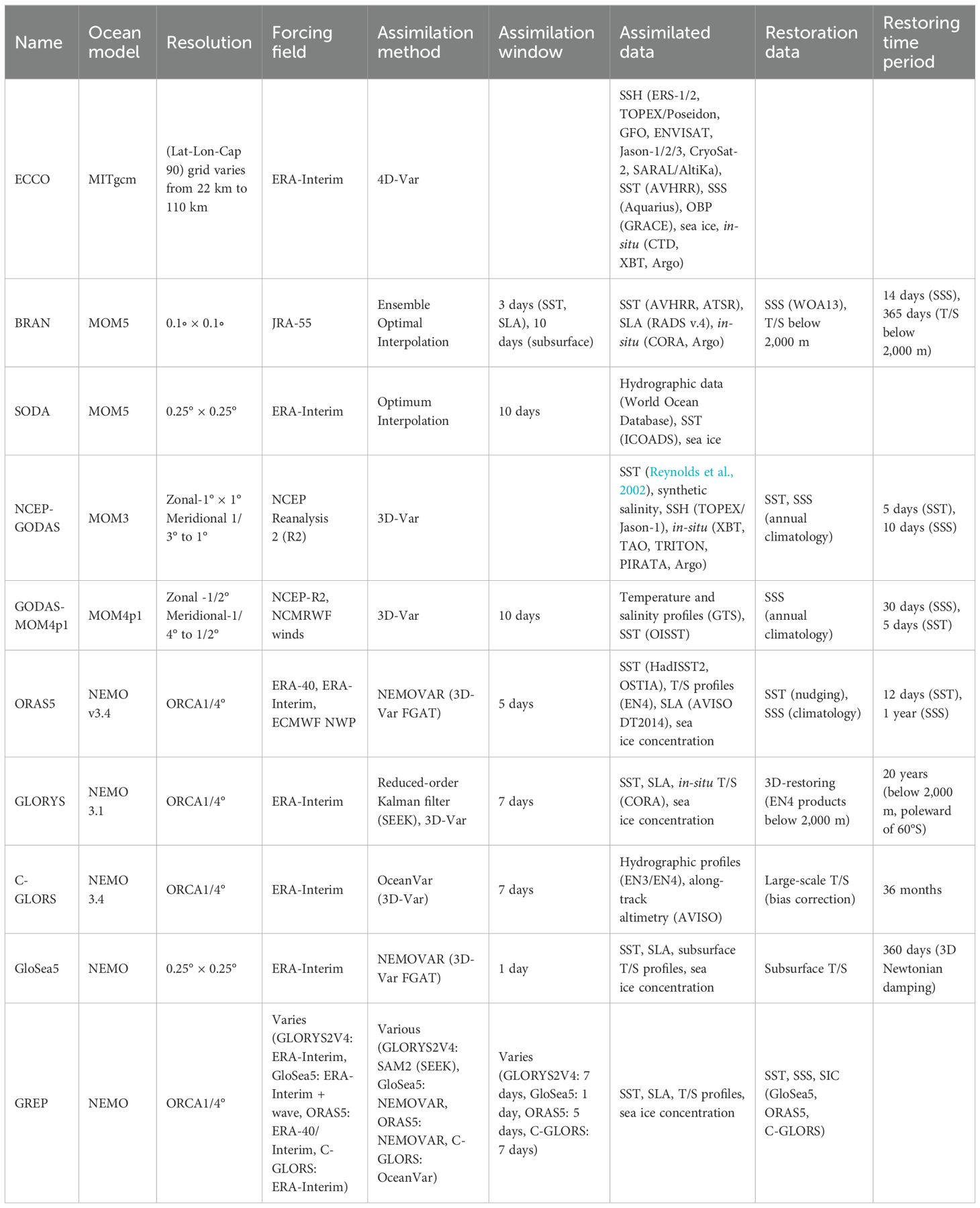
This study evaluates the performance of SST for 10 global ocean reanalysis products, namely, ECCO, Bluelink ocean reanalysis (BRAN), Simple Ocean Data Assimilation (SODA), Global Ocean Data Assimilation System (NCEP-GODAS), GODAS-MOM4p1, Ocean and sea ice ReAnalyses System (ORAS5), Global Ocean Reanalysis System (GLORYS), Global Seasonal forecast System (GLOSEA), CMCC Global Ocean Reanalysis System (CGLORS), and GREP for the northern IO. The details of the reanalysis products used in this study are summarized in Table 1. A detailed description of the reanalysis products can be seen in the supplementary section. The reanalysis SST is validated using SST data from 12 moored buoys from the OMNI network (Acharya and Chattopadhyay, 2019), deployed by the National Institute of Ocean Technology (NIOT, Chennai, India) under the National Data Buoy Program (NDBP). These moorings are located in the Arabian Sea (AS) and Bay of Bengal (BoB) basin (Figure 1). The evaluation was done using 5 m temperature data from the buoy and the reanalysis products. Since the 5-m depth data are not available for BRAN, the average of 2.5 m and 7.5 m was taken as a substitute. It is worth mentioning that the 5-m buoy observed SST was used to evaluate the analysis and reanalysis products since all these products provide the bulk SST. The subsurface SST (SSTdepth, traditionally referred to as a “bulk” SST) considers any temperature within the water column beneath the SSTsubskin, where turbulent heat transfer processes dominate (Donlon et al., 2002). The evaluation time period of the study was restricted to 5 years (from October 2012 to December 2017) due to the availability of OMNI buoy data starting in October 2012 and the ECCO dataset limited till 2017. The analysis and evaluation of the reanalysis SST based on in-situ observational data were performed after regridding all the reanalysis products to 1-degree resolution for a monthly time scale. A search radius of 1 degree was considered at the buoy location, and the values of grid points inside the circle were averaged. This circle was considered by taking into account the watch circle of the buoy. We have also evaluated how the observation-based (or observation analyses) gridded products such as ERSST, Centennial In Situ Observation-Based Estimates of SST (COBE), HadISST, Advanced Microwave Scanning Radiometer-2 (AMSR2), OSTIA, and Optimum Interpolation Sea Surface Temperature (OISST) performed at these buoy locations. Since ERSST has a coarser resolution of 2°, the search radius for this product was chosen as 2°. Later, the best synthetic observation product was used for the spatial analysis of reanalysis SST. Since the SST user community relies more on the high-resolution SST data (e.g., tropical cyclone monitoring, short-term weather forecasting, fishery management), we have also analyzed the high-resolution daily SST from BRAN with the OMNI data.
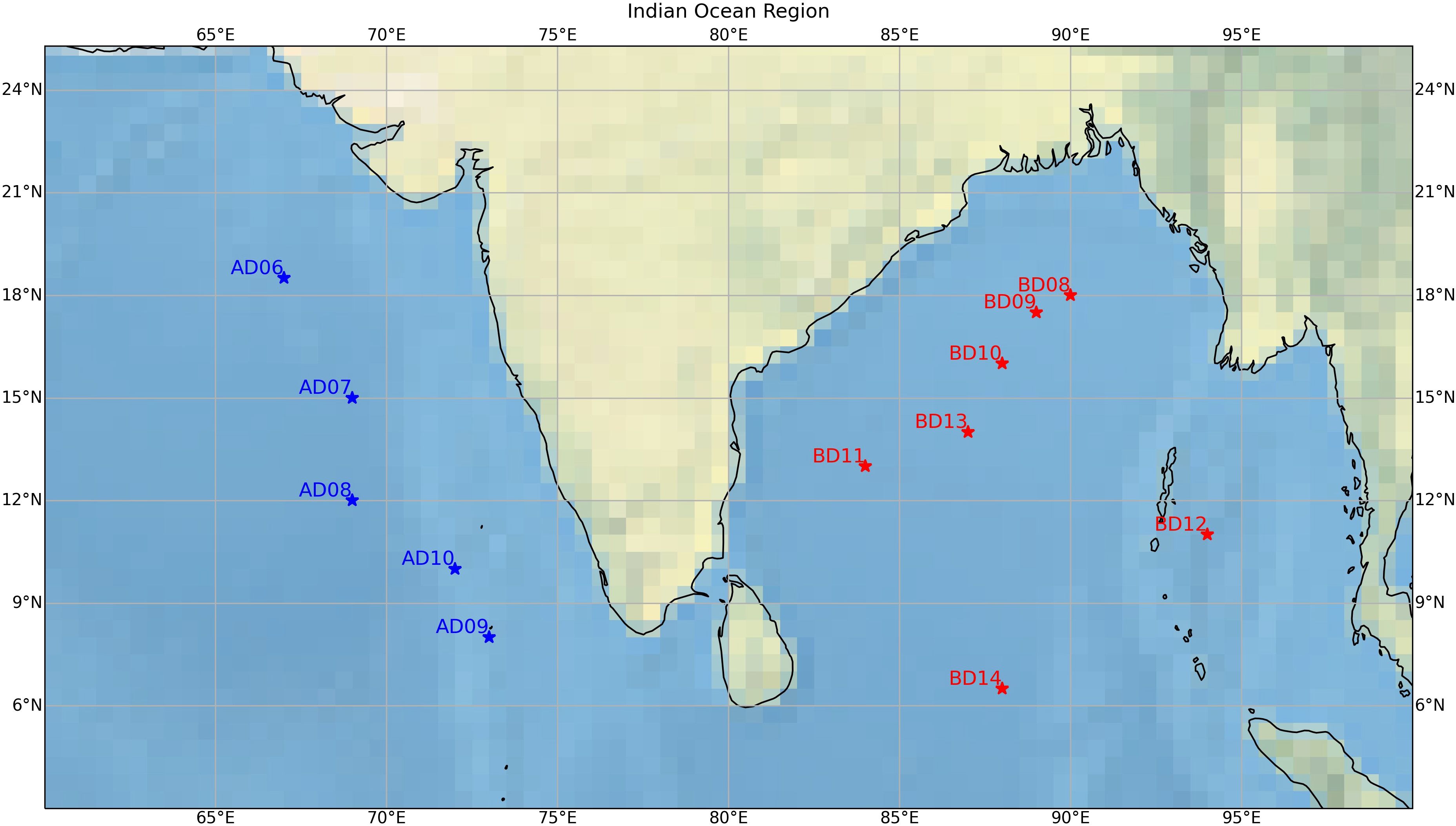
Figure 1. Location of OMNI moored buoys in the Indian Ocean. The blue color stars represent AD buoys in the Arabian Sea and the red star shows BD buoys in the Bay of Bengal.
2.1 Reanalysis products
2.1.1 ECCO
The ECCO reanalysis (Forget et al., 2015; Fukumori et al., 2019) covers the period from 1992 to 2017. It uses the MIT general circulation model (MITgcm), integrating a wide range of satellite and in-situ data, including sea surface height (SSH), SST, sea surface salinity (SSS), and ocean bottom pressure (OBP). The 4D-Var data assimilation method of ECCO ensures that the estimates are physically consistent, satisfying the laws of physics and thermodynamics, which conserves heat, salt, volume, and momentum.
2.1.2 BRAN
The BRAN uses the Ocean Forecasting Australia Model (OFAM) with a 0.1° horizontal resolution (Chamberlain et al., 2021), forced by JRA-55 (Kobayashi et al., 2015; Tsujino et al., 2018) and employs the multiscale data assimilation (DA) approach, primarily using the Ensemble Optimal Interpolation (EnOI) method (Fu et al., 2009; Moore et al., 2019). Observational data such as SST, sea level anomaly (SLA), and subsurface temperature and salinity from Argo profiles are assimilated, with updates to temperature, salinity, and velocities (u, v).
2.1.3 SODA
The SODA3 (Carton et al., 2018) ocean uses the 0.25° horizontal resolution Modular Ocean Model (MOM5), incorporating active sea ice and enhanced topography representation (Carton et al., 2018). This model is forced with ERA-Interim reanalysis (Dee et al., 2011). SODA3 assimilates hydrographic data, including the World Ocean Database and SST data from both in-situ and satellite sources, such as ICOADS version 5 (Woodruff et al., 2011).
2.1.4 GODAS
The reanalysis product by NCEP uses GODAS. It is based on the GFDL Modular Ocean Model version 3 (MOM.v3) and covers a quasi-global domain from 75°S to 65°N, with a resolution of 1° increased to 1/3° in the north–south direction near the equator (Behringer, 2007), and uses 3D-Var assimilation schemes. GODAS is forced by momentum, heat, and freshwater fluxes from the NCEP Reanalysis 2 (R2). The system employs a 3D-Var assimilation method, modified to incorporate synthetic salinity profiles alongside temperature profiles from XBTs, TAO, TRITON, PIRATA moorings, and Argo floats. GODAS provides near-real-time reanalysis data (with a 1-day delay) from 1979 to the present.
2.1.5 GODAS-MOM4p1
The updated Global Ocean Data Assimilation System (GODAS) by Rahaman et al. (2016, 2018) employs the MOM4p1 ocean model (hence GODAS-MOM4p1) with a tripolar grid and 1/4° horizontal resolution forced with NCEP-R2 and NCMRWF winds. This version incorporates submesoscale eddy parameterization to prevent excessive mixed layer depths. GODAS assimilates temperature and salinity profiles from FNMOC USGODAE. Surface temperature is corrected by restoring the model’s first layer temperature to the OISST.
2.1.6 ORAS5
The ORAS5 (Zuo et al., 2019) reanalysis, part of ECMWF’s OCEAN5 system, employs the NEMO v3.4 (Nucleus for European Models of the Ocean) ocean model with a horizontal resolution of 0.25°. The assimilation method uses NEMOVAR to assimilate temperature and salinity profiles, sea ice concentration, and altimeter-derived sea-level anomalies. Key observational datasets include HadISST2 and OSTIA for SST, EN4 for in-situ data, and AVISO DT2014 for sea-level anomalies.
2.1.7 GLORYS2
The GLORYS2 Version4 (Lellouche et al., 2013; Garric and Parent, 2013) reanalysis system is based on the NEMO 3.1 ocean model with a horizontal resolution of 0.25°. The ERA-Interim reanalysis product is used for surface forcing after bias correction in precipitation and radiative fluxes. The data assimilation employs a reduced-order Kalman filter based on the SEEK formulation and a 3D-Var bias correction for temperature and salinity. The system assimilates satellite-derived SST and SLA, in-situ temperature and salinity from CORA, and sea ice concentration. There is no global restoration for sea surface salinity or SST, but 3D-restoring toward EN4 products is applied below 2000 meters.
2.1.8 C-GLORSv7
The C-GLORSv7 reanalysis (Storto and Masina, 2016) is based on NEMO 3.4 having a resolution of 0.25° and is forced with ECMWF ERA-Interim atmospheric reanalysis. The C-GLORS employs the OceanVar data assimilation scheme, which assimilates hydrographic profiles from EN3 and EN4 datasets, as well as altimetric observations. The large-scale bias correction of CGLORS helps mitigate errors due to model parametrization and atmospheric forcing while preserving inter-annual variability.
2.1.9 GloSea5
The GloSea5 reanalysis system (MacLachlan et al., 2015; Blockley et al., 2013) uses a 0.25° NEMO ocean model forced with ERA-Interim reanalysis and employs the NEMOVAR assimilation scheme, incorporating satellite and in situ observations of sea-surface temperature (SST), sea-level anomaly, subsurface temperature and salinity profiles, and sea ice concentration. A 360-day, 3D Newtonian damping is used to correct the long time evolution of subsurface temperature and salinity.
2.1.10 GREP
The GREP (version 1) utilizes four ocean reanalyses developed with the NEMO model on the ORCA025 grid at 1/4° resolution, providing a multi-model ensemble product (Desportes et al., 2017). The contributing systems are GLORYS2V4 (Mercator Ocean, France), ORAS5 (ECMWF), FOAM/GloSea (UK Met Office), and C-GLORS (CMCC, Italy). All reanalyses assimilate SST, sea-level anomaly (SLA), temperature and salinity profiles (T/S), and sea ice concentration (SIC). Key differences include the assimilation methods and windows.
2.2 Observation
2.2.1 Analysis/synthetic observations
2.2.1.1 COBE
COBE version 1, produced by the Japan Meteorological Agency (JMA), provides historical SST datasets essential for monitoring global warming (Ishii et al., 2005). The SST analysis is conducted on a 1° latitude by 1° longitude grid using an optimum interpolation method. COBE analyses utilize data from the Global Telecommunications System (GTS) and drifting buoy data from the Canadian Marine Environmental Data Service and ICOADS data.
2.2.1.2 OSTIA
The UK Met Office OSTIA system (Donlon et al., 2012) is developed to provide surface boundary conditions for high-resolution Numerical Weather Prediction (NWP) models, and it offers daily global coverage of foundation SST. This system integrates data from both infrared and microwave satellites, as well as in-situ measurements from GTS for SST.
2.2.1.3 ERSST
The ERSSTv5 dataset (Huang et al., 2017), a monthly global 2° × 2° SST product, integrates data sources, including ICOADS version 3.0, a decade of near-surface data (above 5 m) from Argo floats, and sea ice from HadISST2. Cross-validations and verifications with modern independent observations indicate that ERSSTv5 offers a better representation of spatial variability across global oceans. ERSST v5 also uses in-situ ship and buoy observations.
2.2.1.4 HadISST
The HadISST dataset offers monthly globally complete fields of SST and sea ice concentration on a 1° latitude–longitude grid from 1871 to the present (Rayner et al., 2003). SST data are sourced from the Met Office Marine Data Bank and GTS from 1982 onward, supplemented by monthly median SSTs from the Comprehensive Ocean-Atmosphere Data Set (COADS) for 1871–1995. The HadISST includes ship and buoy observations as well as satellite advanced very high-resolution radiometer (AVHRR) observations.
2.2.1.5 OISST
The NOAA OISST (Reynolds et al., 2007) blended product, Version 2.1, provides monthly average foundation SST data derived from satellite observations, including data from AVHRR and advanced microwave scanning radiometer. It also incorporates ships, buoys, and Argo float data. This dataset, available from 1981 onward, offers a spatial resolution of 0.25° × 0.25° with a daily temporal interval.
2.2.2 AMSR2 observed SST
The AMSR2 (Wentz et al., 2014) mounted on JAXAs GCOM-W1 satellite offers monthly data on SST (~1 mm), surface wind speed, vertical column vapor, cloud water, and rain rate. Operating from a polar orbit aboard the Aqua satellite, AMSR2 provides comprehensive coverage over global oceans, with its microwave capabilities enabling observation through clouds, except during heavy precipitation.
3 Results and discussion
This study evaluates the performance of SST in various state-of-the-art global ocean reanalysis products. We analyze 10 ocean reanalysis products using 12 independent moored buoy observation data over a 5-year period on a monthly scale. Additionally, to identify the best-performing synthetic observation SST products for spatial analysis in the IO, we conducted a similar evaluation using the same moored buoy data. For the convenience of readers, we present the results for both reanalysis and observation-based products together.
3.1 Evaluation of reanalysis and observed SST with the OMNI buoy
SST drives the deep atmospheric convection in the tropical ocean (Bjerknes, 1969; Gadgil et al., 1984; Graham and Barnett, 1987; Bony et al., 1997a, b), which is determined by heat flux, advection, and mixing in the upper ocean (Vinayachandran et al., 2002). The tropical north IO is notably the warmest part of the world’s oceans just before the summer monsoon onset in April and May (Joseph, 1990; Shenoi et al., 2002). These warm conditions are conducive to active convection (Gadgil et al., 1984; Graham and Barnett, 1987; Sanilkumar et al., 1994). Simulating the absolute value of SST is important for convective activity (Bhat et al., 2004). Hence, any error in the SST products utilized for the evaluation of the atmospheric model or initialization of a general circulation model will have significant implications. Thus, this study aims to see how good the reanalysis and observation-based synthetic SST products are in the north IO.
The monthly averaged SST of each reanalysis product is compared with OMNI buoy data from all the buoy locations. Figure 2 (and Supplementary Figure, Figure S1) shows the SST time series comparison at AD06, AD09, BD09, and BD11 from all 10 reanalysis products along with in-situ buoy observations. All the reanalysis products are able to capture the bimodal seasonal cycle as well as interannual variations. Over the northern Arabian Sea (AS) buoy location, GODAS-MOM4p1 remarkably reproduces the maximum observed SST during May (Figure 2A). The intermodel spread at the AD06 location is less compared to the South Eastern Arabian Sea (SEAS; Figure 2B) buoy location. Almost all models show excess cooling during the peak summer monsoon month of August. The frequency distribution plot (Supplementary Figure S2A) shows lower SST values (25°C–25.5°C) by the reanalysis product, which is absent in the buoy observations over the north AS. On the other hand, the buoy-observed high SST values (30°C–30.5°C) were failed to be captured by half of the reanalysis products. The time series comparison for SEAS at the AD09 location is shown in Figure 2B. This region lies over the mini-warm pool region, which shows the highest SST during May over the global ocean (Vinayachandran et al., 2007). Although all the reanalysis products were able to capture the observed SST variation, the intermodel spread was much higher over this region than in other parts of AS and BoB. ECCO (GLOSEA) over (under)estimated the observed buoy SST throughout the study period at this location. The temporal change of SST at these buoy locations indicated that reanalysis products performed better in the open-ocean regions than near the coast. The interproduct spread in the open ocean was less (Figures 2A, D) compared to the SEAS (Figure 2B) region. The interproduct spread in the open ocean was approximately 0.5°C during winter, whereas it doubled near the coast to approximately 1°C during winter. A consistent spread of 0.5°C was observed between the products throughout the time period of analysis at SEAS (Figure 2B).
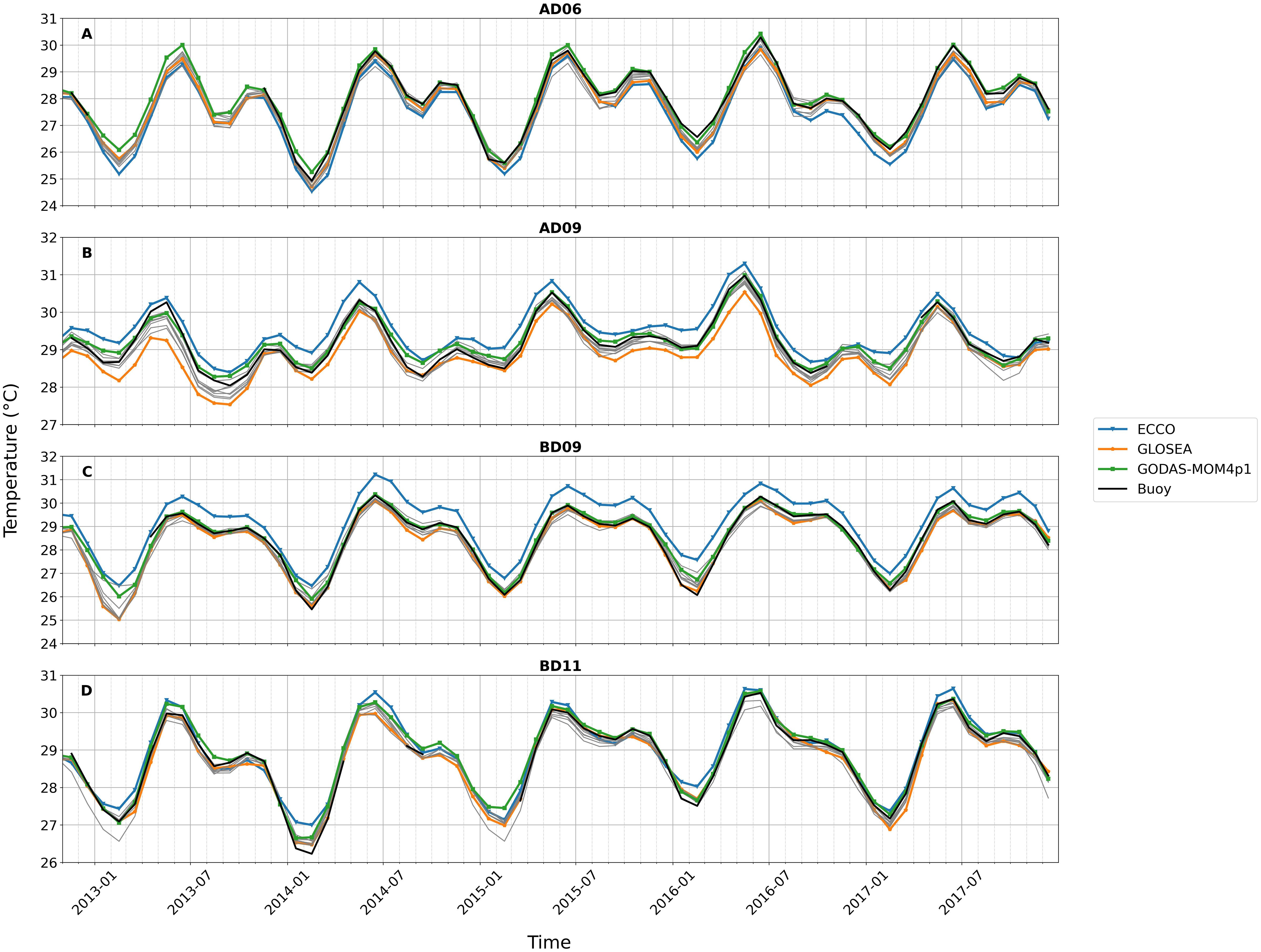
Figure 2. Time series of all the reanalysis products at different buoy locations. (A) AD06 at the northern Arabian Sea, (B) AD09 at the southeastern Arabian Sea, (C) BD09 at the northern Bay of Bengal, and (D) BD11 at the central Bay of Bengal. The colored lines are for ECCO (blue), GLOSEA (orange), GODAS-MOM4p1 (green), and buoy (black), and the rest of the products are given in gray-colored lines (detailed figure for all the reanalysis is given as Supplementary Figure S1).
The analysis of the AS buoys revealed a consistent cold bias in the reanalysis products, particularly during the winter and spring months (Figures 2A, B). In contrast, the northern BoB exhibited a slight warm bias during the winter cooling period (Figures 2C, D). The ECCO reanalysis showed a cooler bias at the AD06 location (Figure 2A), which transitioned to a warm bias toward the SEAS (Figure 2B). Concurrently, GLOSEA displayed a cold bias in the AS. The warm bias in ECCO at SEAS continued into the northern BoB (BD08, BD09) (Figure 2C). The large systematic warm bias in ECCO was slightly reduced over the southwestern BoB buoy location (BD11, Figure 2D). The warming of ECCO in the regions of low salinity due to freshwater inflow may be arising due to the buoyancy, as it tries to maintain a dynamically consistent ocean state estimate (Forget et al., 2015). The thermodynamic structure of the upper ocean is influenced by surface buoyancy, which is mainly contributed by salinity (Vialard and Delecluse, 1998; Durand et al., 2004). Fu et al. (2023) also noted a deviation in ECCO SST, attributing it to the assimilation scheme that prioritizes ocean mass and energy conservation over strict SST constraints. In this study, a time series analysis found that GODAS-MOM4p1 closely aligned with the observed SST at most of the locations. While GODAS-MOM4p1 generally performed better in terms of mean, correlation, RMSE, bias, and standard deviation compared to the other products, there were some locations where other products also outperformed it, as indicated in Tables 2, 3. The colder bias in GLOSEA at SEAS (Figure 2B) may be due to increased mixing arising due to enhanced vertical diffusion caused by the convection parametrization used (Blockley et al., 2013). It is worth noting that all the reanalysis products are very close to observed variations during March–April–May (spring) at all the locations.
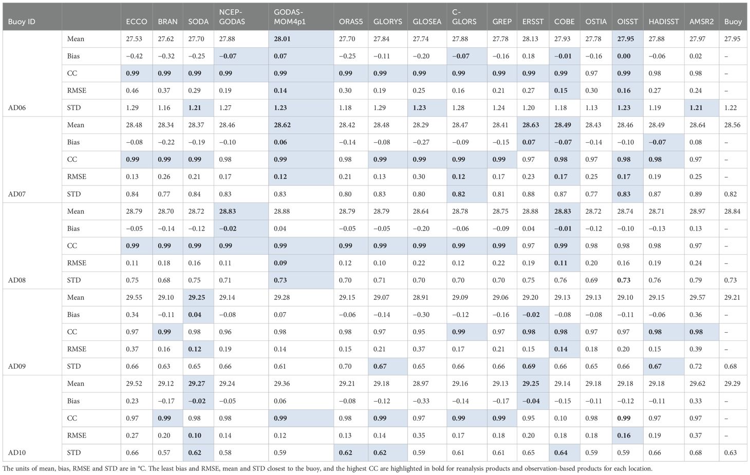
Table 2. The mean, bias, correlation coefficient (CC), root mean square error (RMSE), and standard deviation (STD) for Arabian Sea buoys (AD buoys) calculated for the monthly analysis at each buoy location.
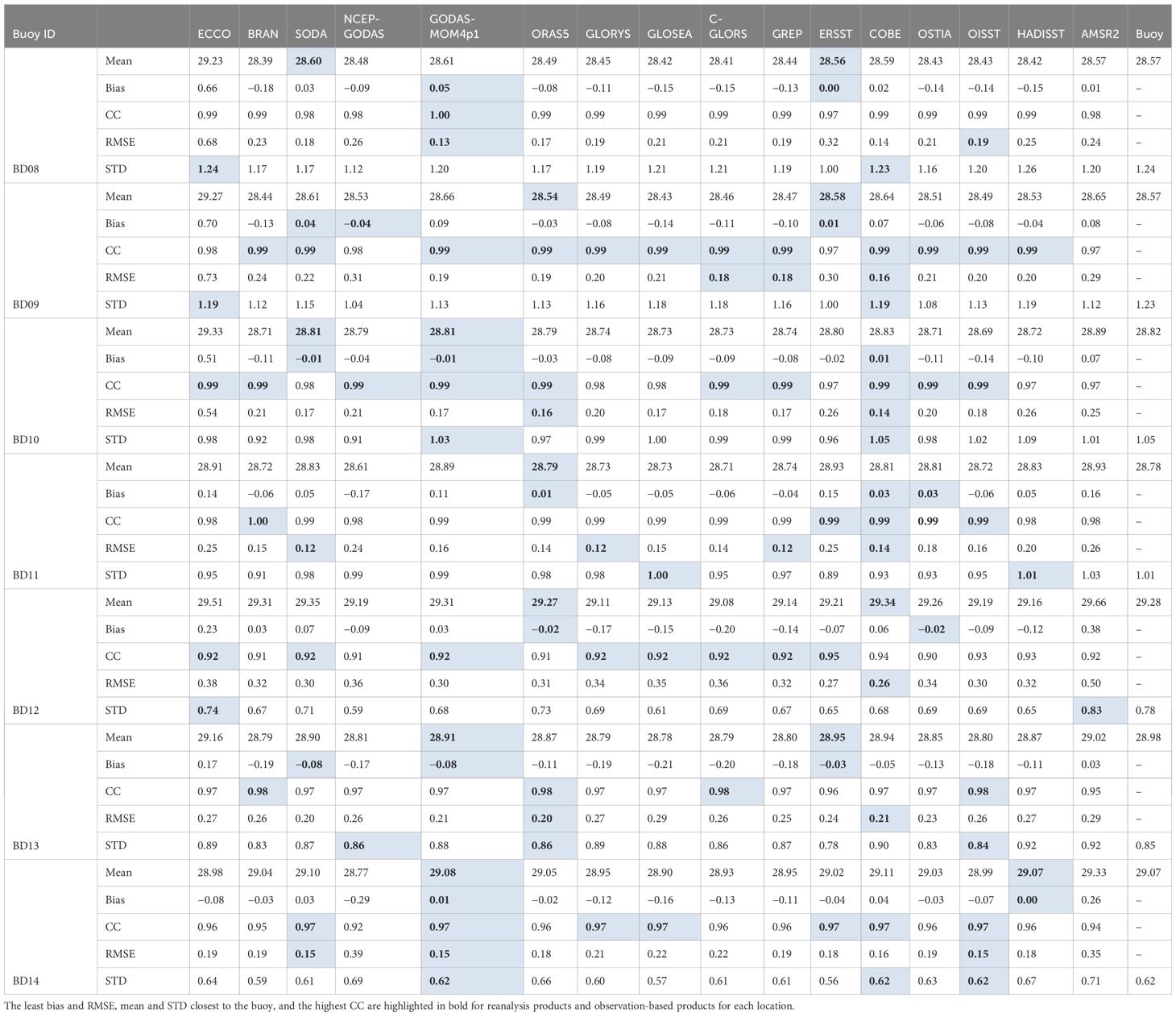
Table 3. The same as Table 2 but for the Bay of Bengal buoys (BD buoys).
The combined mean time series (figure not shown) of all the locations shows that all reanalysis products exhibited a cold bias in the AS throughout the analysis period. The combined effect of the colder bias in the open ocean and the warmer bias in the SEAS resulted in a more accurate performance for ECCO in the AS. However, in the BoB, ECCO consistently showed a warmer bias.
Figure 3 (Supplementary Figure S3) shows the heat map (a visual representation of 2D data using colors to represent values) of the mean and standard deviation (STD) of SST from the buoy and all reanalysis (synthetic observation) products at all buoy locations, as well as the bias and RMSE of the reanalysis product (synthetic observation) with respect to buoy observations. Mean SST from buoy observations is much cooler at the northern AS buoy (AD06) as compared to all other locations. All reanalysis products show mean values closer to observation except ECCO, which is cooler over AD06 and warmer over SEAS (AD09 and AD10). Overall, the mean SST values of GODAS-MOM4p1 were closest to the observation at all buoy locations. The mean observed SST value was the highest at the AD09 and AD10 buoys (SEAS region). Warmer mean SST was also seen in the Andaman Sea (BD12), which is ~29°C. At both these locations, ECCO overestimated the observed values by ~0.5°C. The monthly SST variability was higher over the AD06, BD08, and BD09 buoy locations with buoy observed STD value ~1.2°C (Figure 3B). ECCO overestimated the observed STD values at the AD06 location, whereas the rest of the reanalysis products showed STD closer to the buoy observation. The average bias over the analysis period indicated that GODAS-MOM4p1 had the lowest bias at most buoy locations (Figure 3C). RMSE was the highest for ECCO in the northern BoB region (Figure 3D). It can be noticed that STD values were much higher ~1°C in the northern AS (AD06) and BoB (BD08, BD09) as compared to lower latitude buoys (Figure 3B).
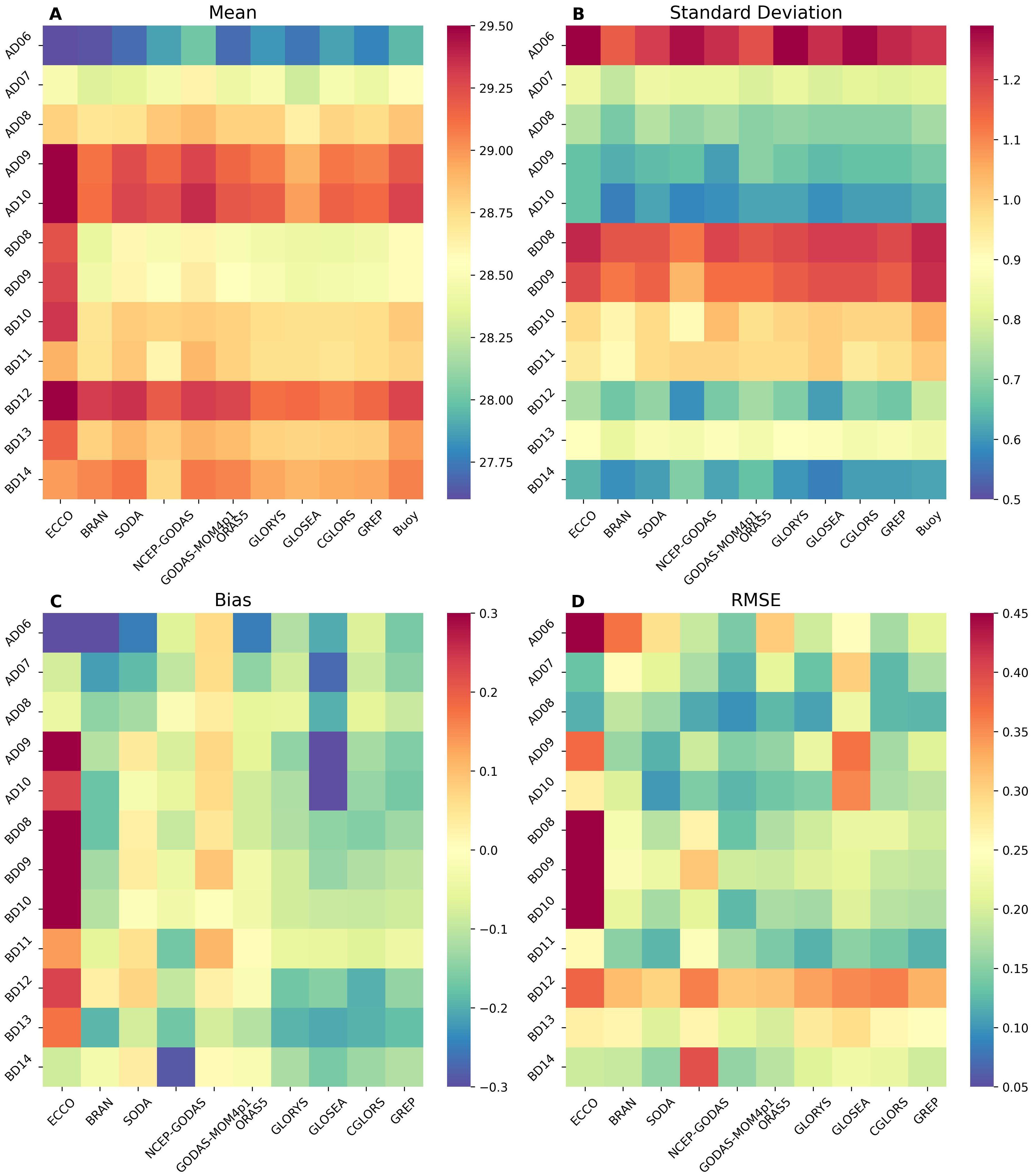
Figure 3. Heatmaps illustrating SST analysis: (A) Mean SST at each buoy location based on reanalysis products and buoy measurements. (B) Standard deviation of SST for both reanalysis data and buoy observations at each buoy site. (C) Average SST bias between reanalysis data and OMNI buoy observations. (D) RMSE of reanalysis SST relative to OMNI buoy data.
Figure 4 (and Supplementary Figure S4) shows the time series comparisons of SST from all widely used synthetic observation products. We showed two buoys over AS and two over BoB for the comparisons. Over the north AS, all observation-based products were able to capture the buoy-observed SST variations (Figure 4A). However, AMSR2 showed systematic warm bias over the SEAS warm-pool region (Figure 4B). The overestimation of SST in AMSR2 could be due to its measurement depth. AMSR2 gave subskin SST, whereas the buoy gave bulk or depth SST (see Section 2). The diurnal SST effect was accounted for in AMSR2 and hence gave higher values than buoy observation. The expected error in the retrievals of SST using a satellite-based infrared sensor was 0.4°C (Shenoi, 1999), and that using the microwave sensor was 0.6°C (Bhat et al., 2004) in the north Indian Ocean. However, the large magnitude of diurnal warming introduced larger errors in the retrieved SSTs, especially in spring (Shenoi et al., 2009). Similar to the reanalysis products, the interproducts spread was more at the AD09 buoy location compared to AD06 over the AS (Figure 4B) for the synthetic observation products as well. Figure 4C shows the SST comparison over BD09, which is located in the northern BoB. This region is very important with respect to the ISMR since the majority of the ISMR rain over central India comes from this region due to the formation of low-pressure systems such as depression and deep depression (Goswami et al., 1999). Similar to the reanalysis products, the observational products also showed a large interobservational spread during summer monsoon and winter. All the observations almost matched the buoy observations during spring (March–May) and early winter (November–December). Similar features are seen over the southern BoB buoy location (BD11), but with interobservational spread reduced during winter (January–February) (Figure 4D).
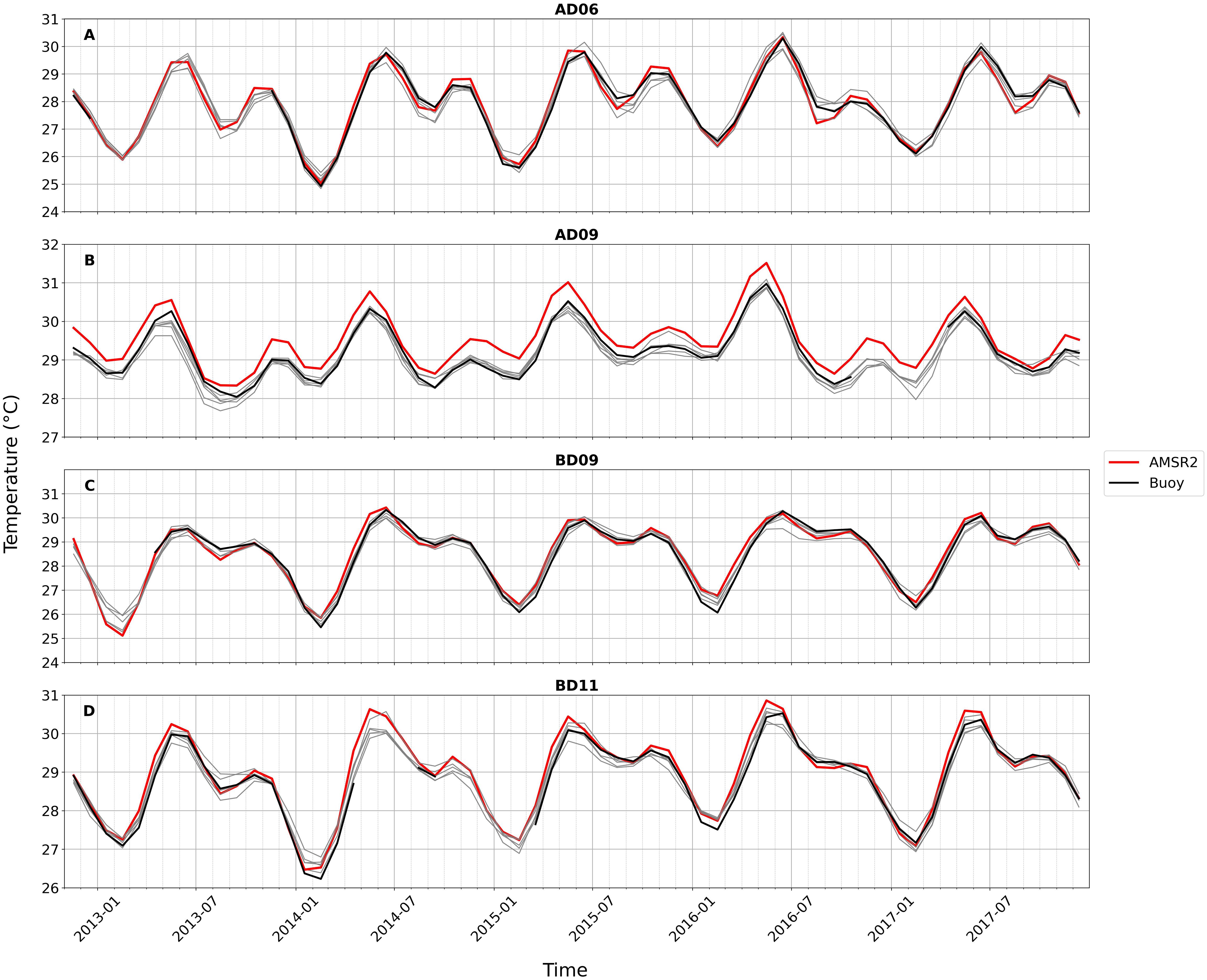
Figure 4. Time series of all the observational products at different buoy locations. (A) AD06 at the northern Arabian Sea, (B) AD09 at the southeastern Arabian Sea, (C) BD09 at the northern Bay of Bengal, and (D) BD11 at the central Bay of Bengal. The colored lines are for AMSR2 (red) and buoy (black), and the rest of the products are given in gray-colored lines (detailed figure for all the observational products is given as Supplementary Figure S4).
The distribution of the reanalysis (synthetic observation) SST (histogram) corresponding to the locations in Figure 2 (Figure 4) is shown in Supplementary Figure S2 (Figure S5). It was seen that the median temperature of GLOSEA was less than the observed in most of the locations. The higher distribution of ECCO SST was warmer than the median observation in most of the locations (e.g., Supplementary Figure S2B). The distribution of OSTIA SST was closer to the observation at the BD11 location (Supplementary Figure S5).
The overall performance of the reanalysis and synthetic observation products was assessed using statistical parameters, including mean SST, mean of bias, correlation coefficient (CC), RMSE, and STD at each buoy location. Tables 2, 3 summarize these parameters for buoys in the AS and BoB, respectively. The best-compared statistics are highlighted in bold in the tables. It can be seen that GODAS-MOM4p1 and SODA performed best with respect to bias and RMSE among the reanalysis products and COBE, as well as OISST from the synthetic observations. All products exhibited a CC above 0.9 for the analysis period. Higher correlations were generally observed in the open-ocean regions (CC above 0.96) and comparatively lower CC near the coast (Supplementary Figure S6), which is less than 0.95. Reanalyses showed poorer performance in regions where the average temperature exceeded 29°C, such as SEAS at the AD09 buoy location and near the Andaman Island coast at the BD12 location. The large spread in CC values can be seen at the AD06 location (Supplementary Figure S6A). From the location-wise variations of CC from all the SST observations and their spread, it can be seen that synthetic observations also showed a similar pattern to that of the reanalysis products (Supplementary Figure S6B).
Figure 5 summarizes the performance of each reanalysis as well as the synthetic observation product when compared with OMNI SST. The product-wise CC and RMSE spread from all collocated reanalysis and observation products from all buoy locations are shown. The box represents the data from the first quartile to the third quartile, and the whiskers extend to show the full range of the data. The horizontal line inside the box shows the corresponding median value. From the figure, we can see that most of the reanalysis products exhibit a higher correlation with a median value above 0.98. In contrast, the median value of SST is generally above 0.97 in the synthetic observation products, with a higher spread, indicating variations in their performance. The GREP ensemble product demonstrated higher correlations at most locations compared to other products, followed by GODAS-MOM4p1, then BRAN (Figure 5A). The better performance of GREP was due to the fact that it is an ensemble product. Previous studies have reported the better performance of ensemble reanalysis products surpassing the observation analyses by partially canceling out the biases of individual reanalysis products (Storto et al., 2017; Toyoda et al., 2017; Ryan et al., 2015). The better performance of BRAN can be attributed to its higher resolution. Earlier studies have found that the reanalysis product with higher resolution tended to simulate the ocean properties accurately (Amaya et al., 2023). It can be seen that the lowest mean CC from reanalysis products was from ECCO (0.98). Figure 5B shows the same from the observations. Except for OISST and COBE SST, all other observations showed CC values lower than that of ECCO. CC values of OISST and COBE SST were even lower than those of GODAS-MOM4p1, GREP, and GLOSEA. The reanalysis products generally performed better, particularly in terms of correlation, than synthetic observation. Analysis of the correlation spread (Figures 5A, B) showed that reanalysis products had higher correlations with less spread than synthetic observation products, indicating superior SST performance when compared with independent buoy data.
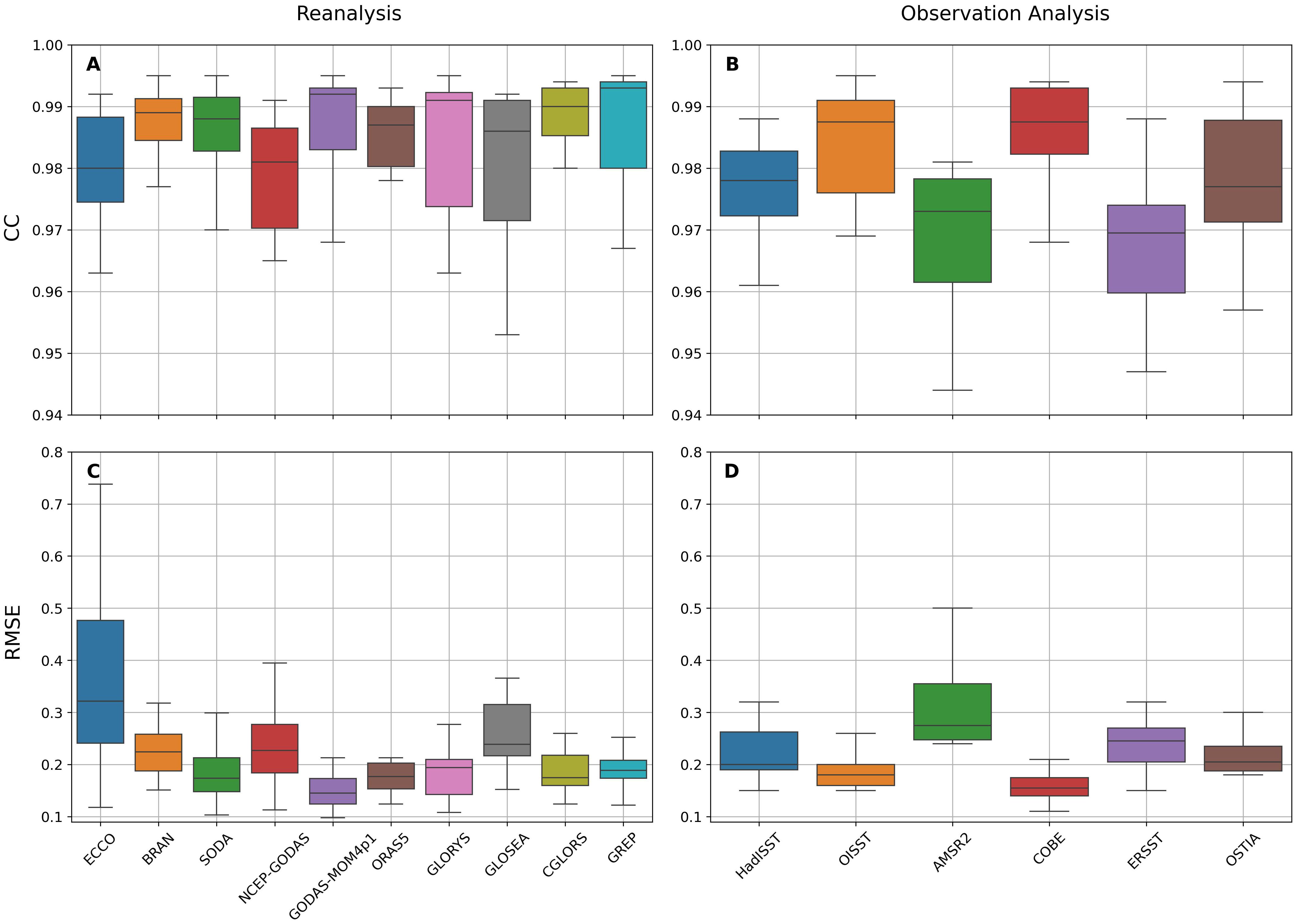
Figure 5. Box and whisker plots for correlation coefficient (CC; A, B) and RMSE (C, D) spread for the SST in reanalysis (A, C) and synthetic observation products (B, D). The box shows the quartiles (25–75 percentile) of the dataset, while the whiskers extend to show the rest of the distribution.
Similar RMSE spreads for all the products from all the buoy locations are shown in Figures 5C, D from reanalysis and synthetic observations, respectively. ECCO exhibited the highest RMSE spread. This was mainly due to simulating warmer SSTs in the SEAS and northern BoB (see Figure 2). For synthetic observation products, AMSR2 showed a higher RMSE spread, primarily due to capturing warmer SSTs near the equator. It is interesting to note that the RMSE of GODAS-MOM4p1 SST was the lowest among all reanalysis as well as all observation products. The higher CC values in OISST and COBE SST also coincided with low RMSE values as compared to other synthetic observation products (Figure 5D).
SODA performed better in the SEAS region with the least average bias and RMSE, although its correlation with SEAS buoys was the second highest. GODAS-MOM4p1 had the lowest RMSE at most locations and showed an STD closer to buoy observations. ORAS5 accurately captured the average temperature in most BoB locations. From Figure 5, the best-performing model in terms of correlation and RMSE spread was GODAS-MOM4p1, which had higher CC and lower RMSE with the least spread for both. This superior performance of GODAS-MOM4p1 as compared to NCEP-GODAS can be attributed to the assimilation of observed salinity profiles as well as restoration with OISST (Rahaman et al., 2016, 2018). It is worth mentioning that NCEP-GODAS and GODAS-MOM4p1 used the same atmospheric forcing, i.e., NCEP reanalysis 2, and the same temperature profiles were being assimilated. The observed variability in terms of STD decreased toward the equator in both basins (Figure 6), which was captured by all the products. Figure 6 is similar to Figure 5, but for the STD, and instead of individual reanalysis, here, we show individual buoy locations, averaged for all reanalysis and synthetic observations. This figure also indicates that STD values over the north AS and BoB were higher (~1.2°C), and its value gradually reduced toward the equator and became half (~0.6°C). Similar variations can also be seen for the BoB buoys (Figure 6A). Synthetic observations also showed similar variations, but the first quartile to the third quartile spreads were large as compared to the reanalysis products, particularly over the BoB (Figure 6B). The better performance of the reanalysis products compared to observation analyses might be due to the physical consistency of the models used for developing the reanalyses. The reanalysis products could capture the underlying physical process that might control the SST, whereas the observation analyses only corrected the satellite SST with in-situ data. The reanalysis products used advanced assimilation techniques as well as bias correction methods. This allows the reanalysis dataset to offer a more reliable and accurate representation of SST.
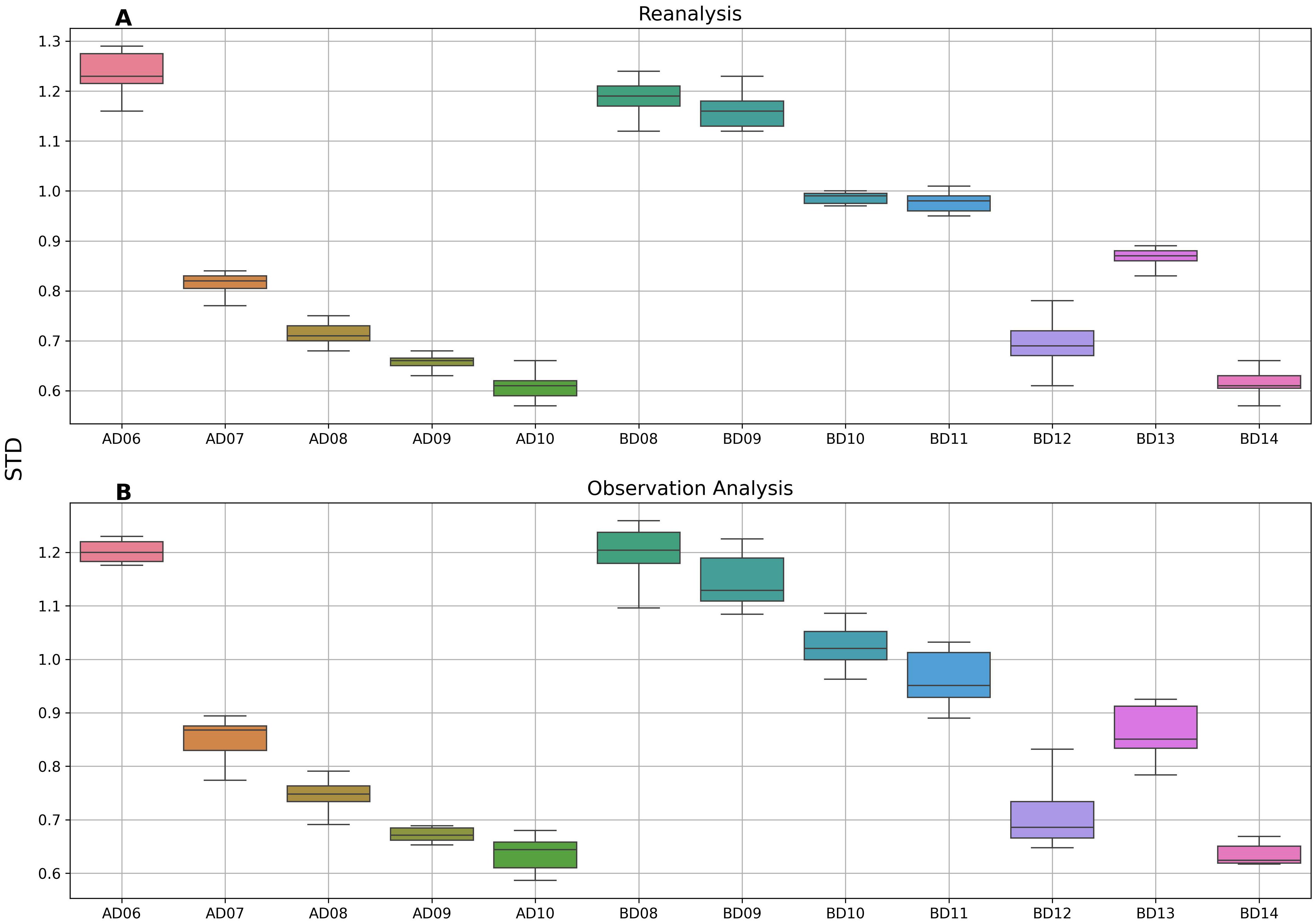
Figure 6. The box and whisker plot showing the spread of standard deviation (STD) of (A) all the reanalysis products at each buoy location and (B) from synthetic observation products at each buoy location.
3.2 Spatial analysis of reanalysis SST
Even though the reanalysis products performed better when compared to synthetic observation products at particular buoy locations, it is essential to understand the spatiotemporal evolution of the SST of the reanalysis products. Since most of the synthetic observation products used satellite as well as in-situ observations, the overall spatial SST pattern was better represented by it. However, there could be errors in the spatial SST pattern of reanalyses because of underlying physics, errors in forcing fields, etc. For the spatial evaluation of reanalysis SST, it is crucial to identify the best-performing synthetic observation product over the IO. Different synthetic observation products differed from each other and were susceptible to errors (Trujillo et al., 2023; Reynolds et al., 2007). Figures 5B, D indicate that COBE SST showed better performance in terms of correlation and RMSE, followed by OISST. The COBE solely relied on in-situ data, and hence, its reliability in the northern BoB is questionable, where a very small number of in-situ observations are available and were incorporated into the COBE analysis. The superior performance of COBE SST over the AD09 buoy location may be due to a lot of XBT section data from the SEAS that went into COBE during its production. So, we mainly used OISST and COBE SST for the spatial analysis.
The coastlines of the north IO are among the most densely populated in the world. Any changes in ocean–atmosphere interactions can significantly impact the millions of people living in these coastal regions (Shenoi et al., 2002) since their livelihood is mainly dependent on the Indian summer monsoon. Understanding and predicting these changes is crucial, especially considering the IO’s strong influence on the monsoon, which is vital for life and agriculture. Given the importance of the IO and its role in the monsoon (Gadgil, 2003; Shenoi et al., 2002), it is essential to accurately understand and forecast ocean–atmospheric conditions (Venugopal et al., 2018) across the entire region. We have included the spatial analysis figures (Figures 7–11) for the summer season (June, July, and August) due to the significance of these months for ISMR. The figures for other seasons were omitted to maintain conciseness. However, the results are included in the text.
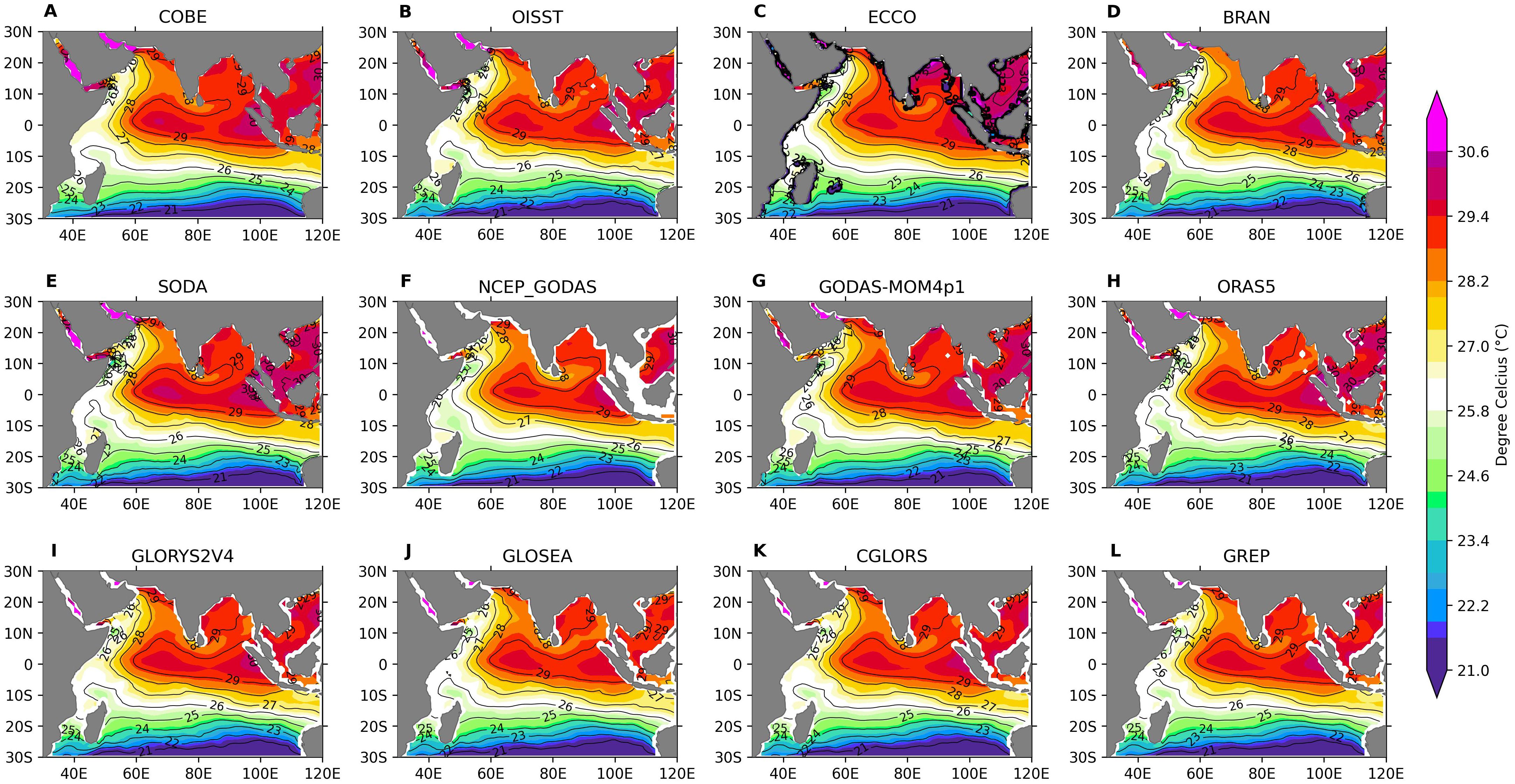
Figure 7. Spatial pattern of mean SST during summer (JJA) from COBE (A), OISST (B), and reanalysis products (C–L).
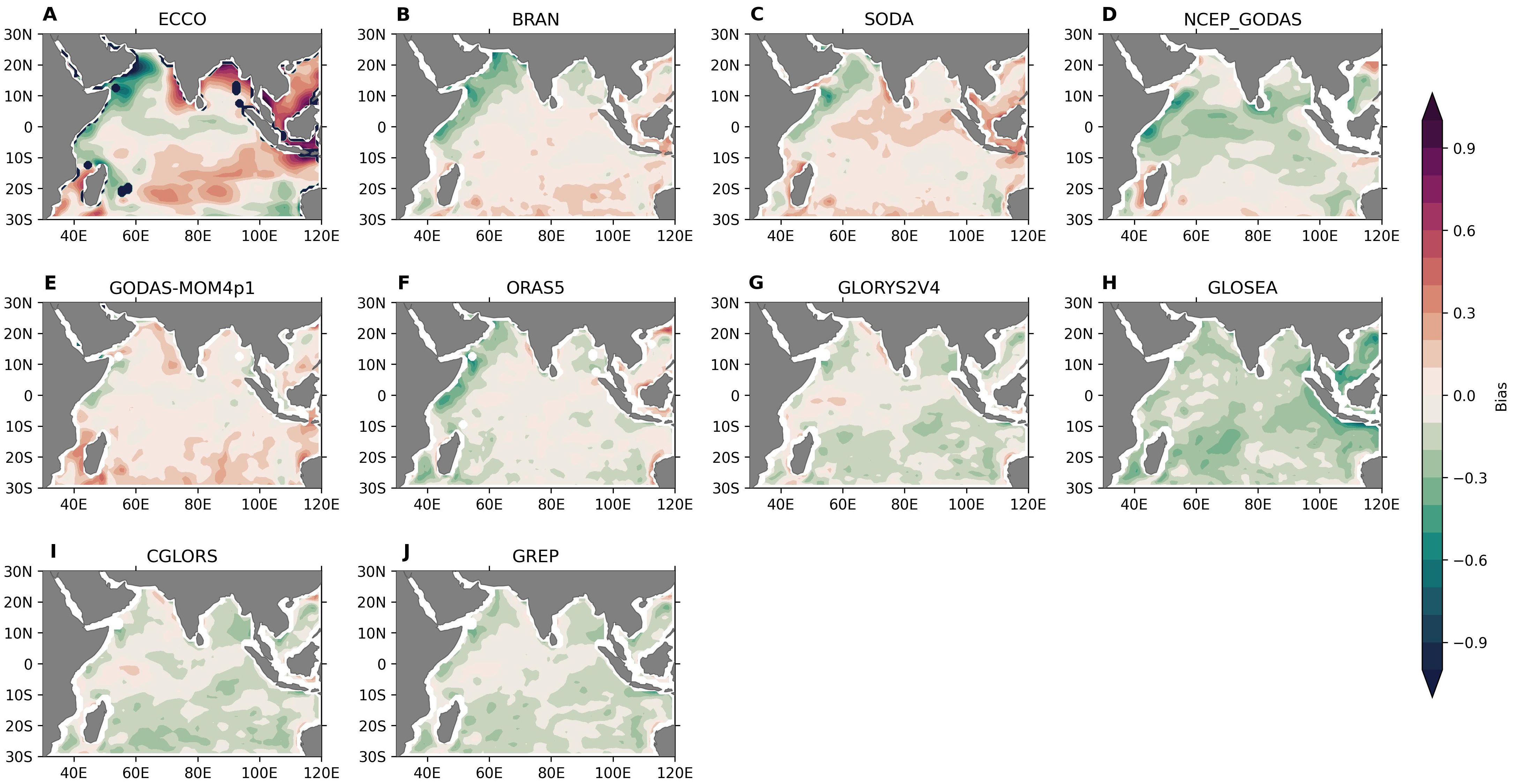
Figure 8. The average bias on a monthly scale for all the reanalysis products (A–J) with respect to OISST observation for the entire period of analysis (October 2012–December 2017).
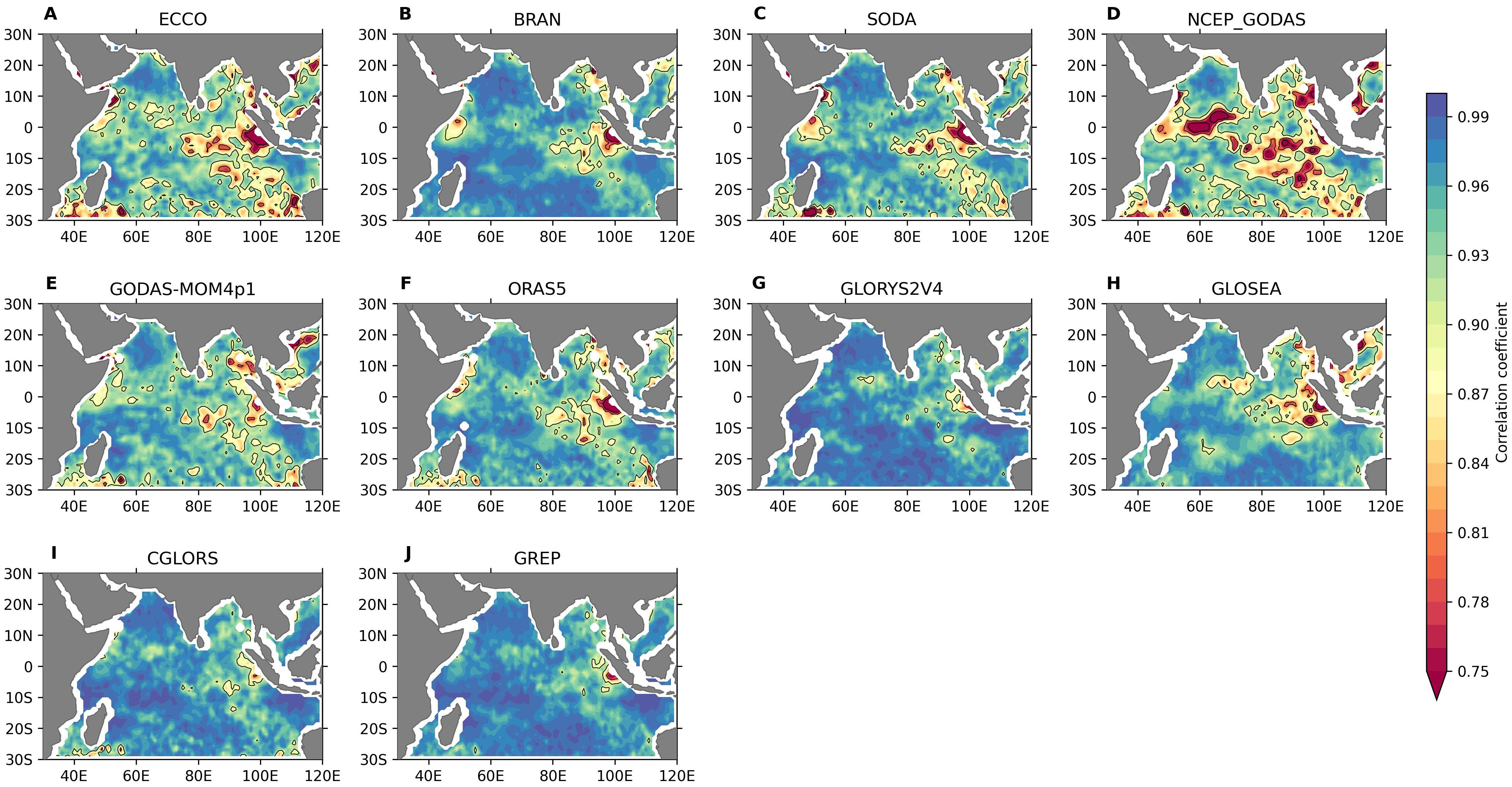
Figure 9. (A–J) Spatial correlation pattern of reanalysis products with the OISST observation during summer (June–August).
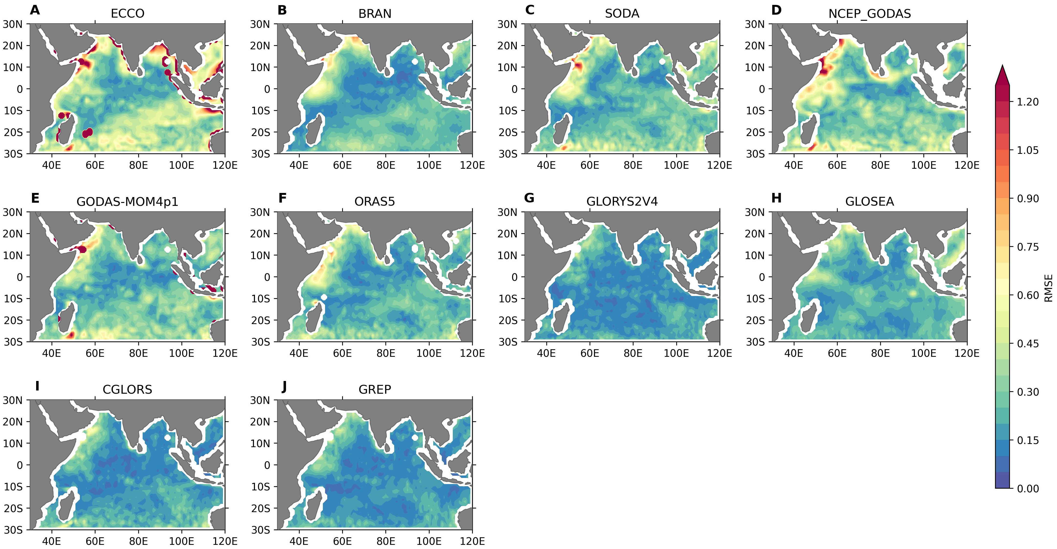
Figure 10. The RMSE of reanalysis products (A–J) with respect to OISST for the summer months (June-August).
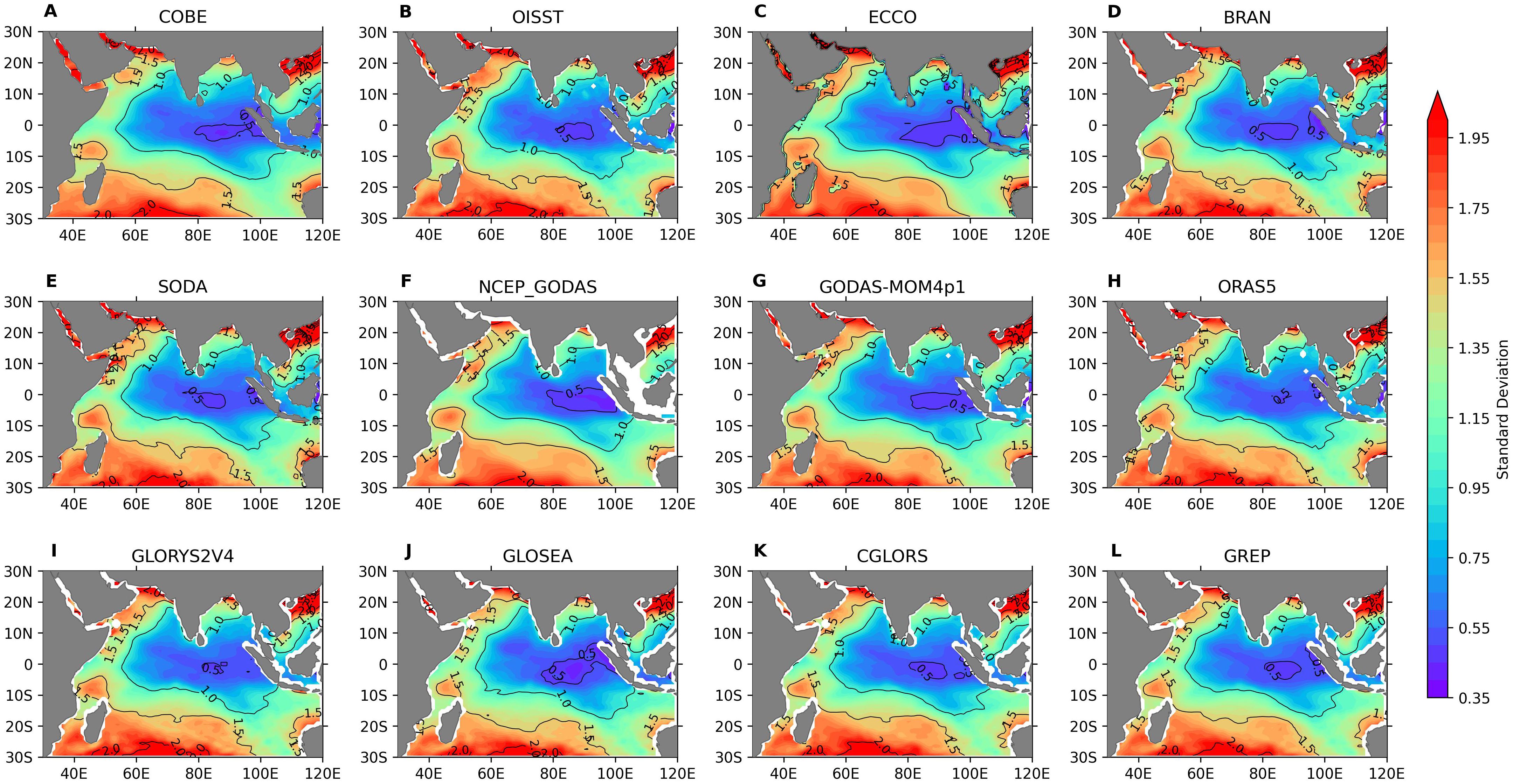
Figure 11. The STD for (A) COBE, (B) OISST, and (C–L) reanalysis products on a monthly scale for the period of analysis (October 2012–December 2017).
The IO gradually warms during the northern hemisphere summer, reaching peak temperatures in May (Joseph, 1990; Shenoi et al., 2002). The warmest temperatures are typically observed approximately within ±5° latitude and 65–75°E, reaching up to 30°C. The tongue-shaped high SST pattern with a dipole SST patch of higher SST (~30°C), one centered at 70°E at the equatorial IO and another at 95°E off Sumatra, was seen in both OISST and COBE SST (Figure 7). This observed tongue-shaped SST pattern embedded with a higher SST patch was simulated by all reanalysis products with slightly varying magnitude. Although ECCO SST was able to capture this equatorial observed SST pattern, it exhibited significantly higher temperatures in the BoB during this period. Another striking difference in the ECCO SST was that the gradient is north–south over the northern BoB instead of east–west, as seen in both the observation products and all the other reanalysis products. ECCO also showed much cooler SST off the Somali coast due to intense upwelling in the model as compared to observations and other reanalysis products. This feature can be seen more clearly in the bias plot shown in Figure 8. This pattern was also seen in the annual mean plot (see Supplementary Figure S7). The annual mean bias in the IO (Figure 8) showed that ECCO has the maximum bias (>1°C) near the coast as compared to other reanalysis products. The reason ECCO showed higher RMSE might be due to the bathymetry used in ECCO along with no SST constraints. Most of the reanalysis products showed a cooler bias in the AS. The cooler bias in the AS in BRAN might be because of the absence of tidal parametrization. SODA had a warm bias reaching up to 0.3°C in the BoB and along the equator and extending to the SEAS. GLORYS showed the least spatial bias, followed by CGLORS. GLOSEA had a basin-wide cooler bias that may arise because of the enhanced mixing resulting from the convection parametrization used.
SODA overestimated the equatorial tongue-shaped warm temperature by more than 0.3°C, while ECCO overestimated the average temperature in the SEAS (close to the western coast of India) of 28.6°C to approximately 29.5°C. Observations also indicated a 1°C warming in the northern BoB in ECCO compared to synthetic observation products. The warmer temperature in the SEAS is because of the inability of ECCO to capture the upwelling on the southwestern coast of India.
During winter (DJF), ECCO also showed higher SEAS temperatures, while GLOSEA depicted lower temperatures (figure not shown). This cooler trend in GLOSEA persisted into spring (MAM), where it, along with NCEP-GODAS, showed cooler temperatures in the equatorial region. Accurate SST representation during this period is crucial for the formation of moisture-laden clouds, which are essential for monsoon onset and ISMR. During summer (JJA), ECCO failed to capture the cooler temperatures at the southern tip of India, while NCEP-GODAS overestimated them (Figures 7C, F). The overestimation of the cooling in the NCEP-GODAS was aided by the unrealistic representation of the coastal Kelvin wave (Rahaman et al., 2014, 2020) and coastal currents, which might have resulted due to the unrealistic representation of bathymetry (Rahman and Rahaman, 2024) and assimilations of synthetic salinity profiles. In fall (SON), the equatorial warm tongue extending from the Sumatra region to 65°E was absent in ECCO. Instead, ECCO displayed a warm tongue structure extending from the equator to the western coast of India, with warmer near-coast temperatures. Although GLOSEA and NCEP-GODAS showed less warming compared to observations, their patterns were similar to the observed.
Monthly bias with respect to OISST and COBE revealed that none of the reanalysis products were able to reproduce the mean SST near the coast. This could be due to the unrealistic representation of bathymetry and mixing schemes, which resulted in the unrealistic coastal Kelvin wave propagation, an issue previously reported by Rahaman et al. (2014, 2020) and Rahman and Rahaman (2024). It is also worth mentioning that even the synthetic observations also suffered large errors in the SST retrieval near the coast (Lee and Park, 2020). Hence, extensive research is needed to generate accurate SST data products near the coast. ECCO exhibited a warm bias in the BoB and a cold bias in the AS, reaching up to 1°C during all months. The CC in the IO region was above 0.9 for most regions across all reanalysis products with OISST and COBE SST (Figure 9). Lower correlations were observed near the Sumatra coast except in GODAS-MOM4p1, GLORYS, CGLORS, and GREP. During winter, correlations decreased near the Indian coast in SODA and GODAS-MOM4p1 and also in the open ocean along 10°S and 7–8°N for ECCO and NCEP-GODAS. Even though the correlation was the highest in most regions during spring, the equatorial eastern IO and the southwestern coast of India showed reduced correlations. The correlation was inappreciable near the equator in NCEP-GODAS and GLOSEA, with correlations below 0.75. Figure 9 shows the correlation of reanalysis products with OISST during summer (JJA). The correlation was lower in the eastern equatorial IO, especially near Sumatra, in all the reanalyses. The correlation with COBE in the northern BoB was also lowest during this time, probably due to the absence of in-situ data in this region (Supplementary Figure S8). The NCEP-GODAS showed a low correlation over the western equatorial IO. This pattern was not observed in any other reanalysis products. The Andaman Sea also showed low CC values in all reanalysis products with varying magnitude, with NCEP-GODAS showing the least among all. This reduction in the correlation over the Andaman Sea may be due to the model configuration as well as a lack of temperature and salinity profiles over this region, which was used for the assimilation.
Figure 10 shows the spatial distribution of average RMSE for the summer months (JJA) of all reanalysis products with respect to OISST. All products showed low RMSE values over equatorial IO, BoB, and southern AS. ECCO and MOM-based reanalysis products showed higher RMSE over the western equatorial IO, Somalia Coast. These reanalysis SSTs near the coast showed higher RMSE compared to the open ocean, with NCEP-GODAS reaching up to 0.6°C near the southern tip of India. Higher RMSE (>0.6) was seen near the Indian coast as well as western AS in ECCO. These results also corroborated the finding of Fu et al. (2023), who showed large errors in the coastal waters, western boundary currents, and Antarctic Circumpolar Current area associated with the poor representation of strong non-linear dynamic processes and the displacement of SST fronts over these regions from six widely used reanalysis SST products. They also found that the basin-wide RMSE was the least in GREP. Seasonal analysis showed that the highest RMSE values were in the northern BoB and near the western coast of India in ECCO, reaching more than 1.2°C during summer (Figure 10) and spring (figure not shown). Amaya et al. (2023) and Trujillo et al. (2023) showed that temperature and salinity in the reanalysis were affected by coastal bathymetry. Recently, Rahman and Rahaman (2024) have shown similar results over the coasts of India. This study also showed that bathymetry changes significantly affect coastal currents and accurate bathymetry is needed for the realistic simulations of temperature, salinity, and currents near the coast. The larger RMSE values near the coasts for most of the reanalysis products advocated the need to represent realistic bathymetry in the global ocean models. During spring, BRAN exhibited a higher RMSE of over 0.5°C in the northern AS. Despite being a high-resolution model, the larger RMSE in the AS SST during this time might be due to the lack of tidal mixing in this region as this region has the highest tidal amplitude in the IO (Figure 4 of Shebalin and Baranov, 2020). In summer (Figure 10), all MOM-based reanalysis products and ECCO showed higher RMSEs near Sumatra and Oman, whereas the NEMO-based products had lower RMSE. The fall RMSE patterns were similar to the annual average conditions, with ECCO showing an RMSE of approximately 1°C near the Oman and BoB coasts and GLOSEA showing an RMSE of 0.6°C to 0.7°C near Sumatra.
Figure 11 shows the monthly mean STD from all reanalysis products and two observational-based synthetic products, OISST and COBE SST. The STD showed that, on average, the variability was the least in the equatorial eastern IO, and the highest was in the northern AS and BoB. Large STD values were also seen near the Somalia coast. This was mainly due to the upwelling that occurred during the summer monsoon season. These large STD values over the Somalia coast is mostly contributed from the JJA STD values (Supplementary Figure S9). All the reanalysis products were able to capture the synthetic observation spatial distribution of STDs over the north Indian Ocean. The maximum observed variability was seen near the Oman coast, with a magnitude reaching 2°C during summer (Figure 11).
3.3 Evaluation of daily reanalysis SST
In the previous sections, we showed the monthly SST comparison of all the reanalysis products. The NWP user community mainly relies on high temporal resolution SST for the boundary conditions. So, it is essential to understand the performance of reanalysis on a daily scale. However, most of the reanalysis products provide monthly products. In this section, we compare the daily SST data from the BRAN reanalysis product as it has high temporal and spatial resolution data among the 10 reanalysis products used in this study. The analysis period was chosen from 2015 to 2017 due to the continuous availability of OMNI buoy data in most of the locations. The daily SST was analyzed using the same methodology adopted in Section 3.1. Table 4 summarizes the statistical analysis for the daily and monthly BRAN SST with OMNI buoy from 2015 to 2017. It was seen that the monthly SST performance is better in terms of CC and RMSE. The daily SST correlation was less than the monthly SST, and the daily RMSE values increased as compared to monthly values (Table 4). However, the average bias for the daily product was less compared to the monthly SST product.
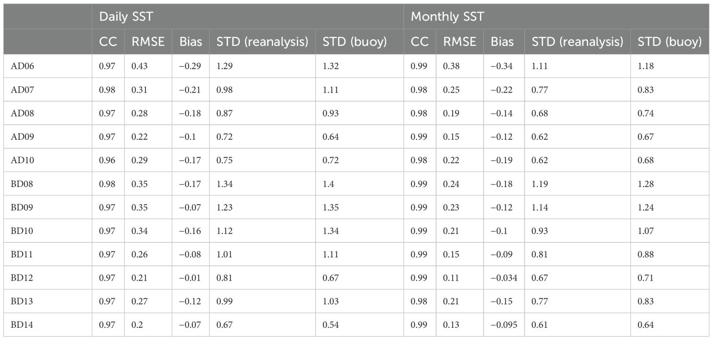
Table 4. Statistical analysis of daily and monthly BRAN data with OMNI buoy during the time period 1 January 2015 to 31 December 2017.
From the time series analysis, it can be seen that the BRAN SST was able to capture the daily variations in SST very close to the buoy SST variability (Figure 12). As seen in the monthly analysis, in the AS, there was a slight cool bias of reanalysis SST, especially during winter (Figures 12A, B). Even though BRAN could capture the sudden cooling events, it was slightly underestimated. The highest bias was seen with respect to moored buoy observation during these sudden cooling events. One such cooling event that happened in the AS was because of the passing of cyclone Ockhi by the end of November 2017. The BRAN SST captured the cooling at all four buoy locations, as in the observation data, with a warm bias (Figure 12B). The highest bias was seen at the SEAS (AD10) with 1.5°C. The average bias in all the buoy locations was negative (Table 4). The CC of the daily BRAN SST in all the buoy locations was higher than 0.96, with the least in the SEAS (0.96 at AD10) and the highest in the open-ocean region (AD07 and BD08 with 0.98). The variability of SST was captured quite well in the reanalysis.
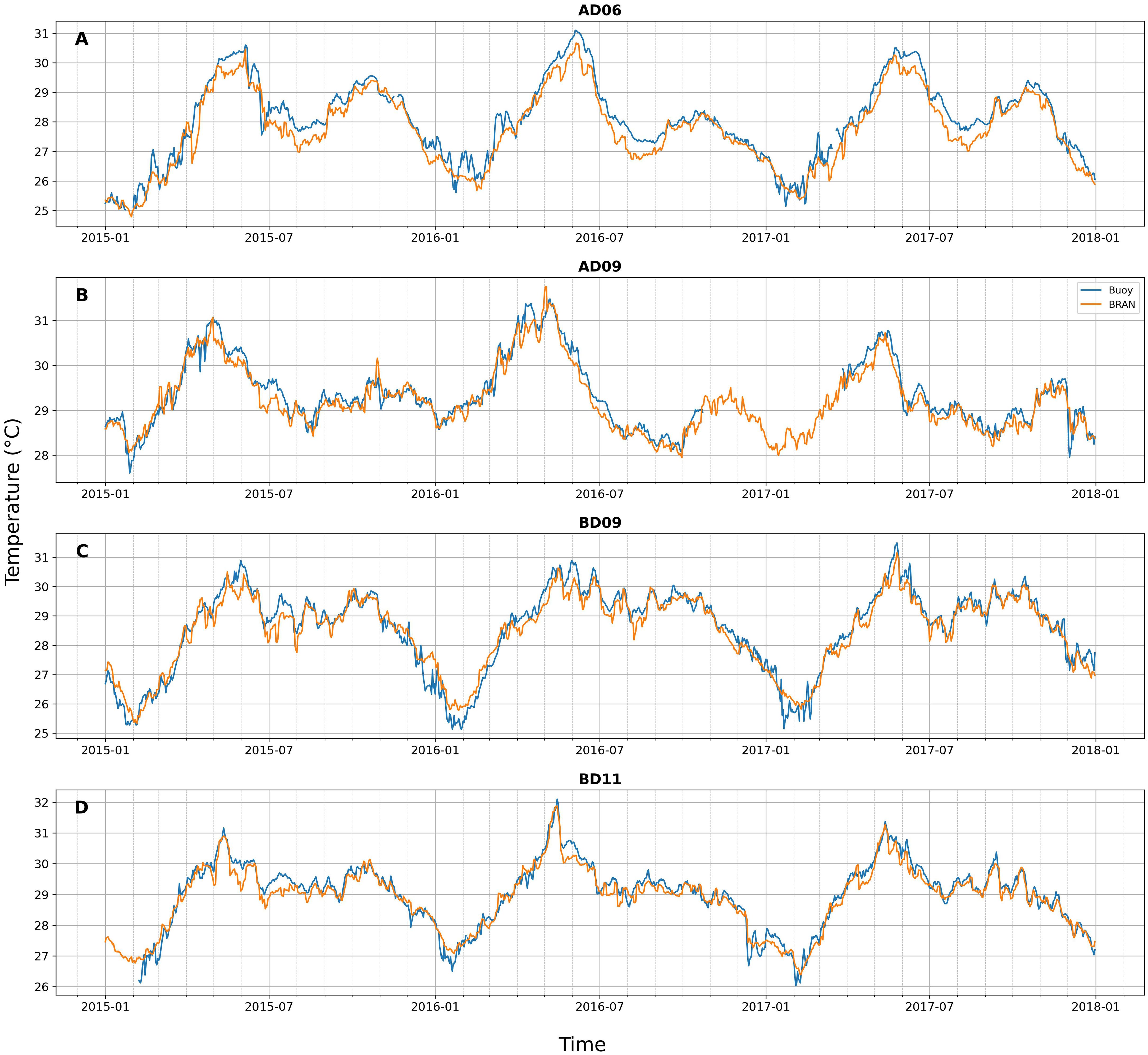
Figure 12. Time series for daily data at locations (A) AD06, (B) AD09, (C) BD09, and (D) BD11 for BRAN SST and OMNI buoy SST.
The seasonal analysis was done for the daily BRAN SST to understand the performance of the reanalysis product in each season. It was seen that the least correlation in most of the region was observed during winter. During this time, CC was less than 0.9 in the BoB and SEAS. During spring, the CC in all the 12 regions was above 0.9, with the least in SEAS with CC 0.91 and 0.93 for AD09 and AD10, respectively. During summer, the correlation in the AS improved, but in most of the BoB locations, CC was less than 0.9. During the fall, the correlation was mostly above 0.9, but in the BD12, CC had the lowest value of 0.84. The average seasonal bias in all the locations showed that it is primarily negative, especially in the AS (more cooling/cold bias). Meanwhile, in the BoB, the averaged bias was mostly positive (warm bias) during DJF. During SON (fall), cold bias persisted in all the locations except BD12. The RMSE was the highest during spring when the RMSE in most of the regions was greater than 0.3°C and the least during autumn. The variability in the spring was underestimated in most of the locations, and the variability in the BD14 location was slightly underestimated in all seasons. The overall statistics in Table 4 show better accuracy on monthly mean SST as compared to daily SST. Temporal averaging over a month smoothed out short-term fluctuations and random noise in daily measurements and made monthly SST data valuable for studies focused on seasonal, interannual, and decadal variability studies. While daily SST data are crucial for short-term weather forecasting and applications that require high temporal resolution, the increased accuracy of monthly data might be more useful for initializing long-term climate models and for model assessment studies where daily variability is less critical. The result also indicated that monthly data are preferable in applications prioritizing accuracy over resolution.
4 Summary and conclusion
The ocean reanalysis products are historical reconstructions of time-varying three-dimensional ocean states based on observations and numerical models. They are more accurate than stand-alone model simulations and have greater coverage than in-situ observations. These products are widely used to study ocean variability, circulation, air–sea interaction, etc. and also to provide the initial conditions for weather forecasting models. Ocean reanalyses are used to initialize the coupled models for the subseasonal to decadal predictions (Pokhrel et al., 2024; Storto et al., 2019) and support observational network monitoring, climate index tracking (e.g., ENSO, IOD), and model evaluation. NWP models rely on SST as a boundary condition, and a poor representation of these can cause forecast uncertainties (Schepanski et al., 2015). Senatore et al. (2020) emphasized that accurate SST representation in the Mediterranean is crucial for improving precipitation forecasts, particularly in regions with complex air–sea interactions and coastal orography. Therefore, a high-accuracy SST dataset, both near the coast and in the open ocean, is crucial for the effective initialization of NWP models.
Despite the importance of reanalysis products, studies on an independent evaluation of these reanalysis products are scarce, particularly the SST products. The reanalysis products inherit errors due to model physics, forcing fields, errors in the observation system, assimilation schemes, etc. Balmaseda et al. (2015) compared different global reanalysis products for ocean heat content, steric height, sea level surface heat fluxes, mixed layer depth, salinity, depth of 20-degree isotherm, and ocean sea ice near Canada. To the best of our knowledge, the evaluation of SST from these reanalysis products over the north Indian Ocean has not been carried out. Hence, in this study, we focused on the assessment of the performance of north Indian Ocean SST from 10 different widely used state-of-the-art reanalysis products. The SST from the reanalysis products is compared with the observational data from 12 OMNI moored buoys in the northern IO on a monthly scale for 5 years from October 2012 to December 2017. Additionally, the performance of six observation-based synthetic SST analysis products was also evaluated.
The reanalysis SSTs we evaluated were from ECCO, BRAN, SODA, NCEP-GODAS, GODAS-MOM4p1, ORAS5, GLORYS, GLOSEA, CGLORS, and GREP. During the same period, analysis was also carried out from five observation-based synthetic products, namely, ERSST, COBE, OISST, OSTIA, and HadISST, and one observed SST from AMSR2 to understand the best-performing observation product in the IO region. The analysis shows that the reanalysis products captured the buoy-observed SST variability with good accuracy. The CC of reanalysis SST is higher than 0.9 for all the products at every location, with a higher correlation in the open ocean and a comparatively lower correlation near the coast. The AS winter cooling is overestimated (cold bias) in all the reanalysis products, but in the BoB, during winter, the reanalysis products mostly exhibit a warmer bias. The interproduct spread is less in the open ocean, whereas it is more near the coast and in the southeastern AS. The interproduct spread is the highest at the AD09 buoy location, which is located in the mini-warm pool region over the southeastern AS. ECCO SST is an outlier among all the reanalysis products with consistently systematic warm bias in all buoy locations. The overall statistics show that GODAS-MOM4p1 and GREP perform best among all the products. The reanalysis products perform better than the observations in terms of spread in correlation and RMSE. The synthetic observation shows a similar comparison to that of reanalysis SST. However, overall statistics show that reanalysis performs slightly better than observation-based products. The AMSR2 SST shows systematic warm bias over most of the buoy locations. This could be due to the fact that AMSR2 measures subskin SST, whereas all reanalysis and synthetic observations are SST depth (or bulk SST), similar to the reference buoy observations used for the evaluation. COBE and OISST perform best among the synthetic observation products. The variability (in terms of STD values) of the SST products from reanalysis and synthetic observations shows higher values over the north AS and BoB, and they gradually decrease toward the equator.
The performance of reanalysis SST with OMNI buoy SST has been observed to be seasonally dependent, with reanalysis products more accurately capturing the springtime SST (MAM) compared to the monsoon and winter seasons. This variation in performance is likely linked to differences in wind speed. Xie and Philander (1994) explain that wind influences SST through mechanisms such as momentum transfer to the ocean, wind stirring, and surface latent heat flux. Recent observations from eddy covariance data in the Bay of Bengal have provided new insights into these fluxes. It was found that for moderate wind speeds (6–8 m/s), the latent heat transfer coefficient calculated using the COARE algorithm aligns well with observed values. However, discrepancies arise at lower and higher wind speeds (unpublished data). Most models currently employ constant parametrization of exchange coefficients, which tends to align more closely with observed values during spring. To address these seasonal discrepancies, a flux calculation algorithm that accounts for seasonal variations is necessary. Storto et al. (2019), in their review study on the challenges of ocean reanalysis, pointed out that air–sea flux errors, inadequate model resolution, and parameterizations are other non-trivial problems to mitigate the drift and bias. This study revealed that as far as SST reanalysis is concerned, probably rather than model resolution, it is the atmospheric forcing and the bulk algorithm errors that play a crucial role.
All the products show a very good match with the buoy observations during April for all the years. However, the intermodel spread is much higher during the summer monsoon and is the highest during winter. Since all the product’s SST is assimilated and also relaxed to the observed SST in the top model layer, we would expect bias and errors to be independent seasonally. However, we saw that the intermodel spreads are not uniform in all seasons. This implies the deficiency in the forcing fields as well as the possible errors in the turbulent heat flux computation using bulk algorithms. The other aspects that could be affecting the mixed layer depths are, in turn, dependent on the mixing schemes used in the individual models. This aspect opens up the possibility of improving the bulk algorithm and seasonal-dependent turbulent closure schemes. A recent study by Jampana et al. (2018) shows that during the post-monsoon period, the buoyancy frequency perturbations are more critical than shear perturbations in driving unstable events. In winter, the unstable events are influenced by both the buoyancy frequency and shear perturbations. Hence, we found that regional and seasonal dependent mixing schemes need to be incorporated into the model physics.
The spatial evaluation of reanalysis products with OISST shows that reanalysis products perform better in the open ocean than near the coast. ECCO overestimates the SST in the SEAS and northern BoB, whereas SODA, on the other hand, overestimates the equatorial warm tongue. The cooler temperature at the southern tip of India during summer is overestimated by NCEP-GODAS, in contrast to ECCO, which shows a warmer bias there at the same time. ECCO shows cooler SST near the Somali coast and off the Oman coast. Similar cold bias was also observed for the MOM-based model BRAN, NCEP-GODAS, SODA, and ORAS5, which is based on the NEMO model. The basin-wide RMSE value is the least in GREP among all the products. Similar to bias, the RMSE values are much higher near the Somali coast for the ECCO and MOM-based reanalysis products. The resolution effect can be seen with reduced RMSEs in BRAN and MOM4p1-GODAS as compared to NCEP-GODAS. The poorer performance of reanalysis products near the coast can be attributed to the unrealistic representation of bathymetry, which leads to the inability to capture the realistic coastal Kelvin waves. The basin-wide spatial distribution of CC values is higher in all the products (>0.9). However, it shows much comparatively lower values in MOM-based products, with NCEP-GODAS showing much lower values of ~0.7.
For climate and seasonal scale applications, monthly SST is used. However, for the intraseasonal and synoptic scale application, daily SST is required. Hence, daily SST from BRAN is analyzed to understand the performance of high-resolution daily SST. It was observed that the reanalysis could very well capture the observed SST, but the sudden changes in the observed SST are not accurately captured. Similar to the monthly analysis, the daily SST also shows a cooler bias in the AS. In comparison with the monthly analysis, it was seen that the RMSE increases in the daily reanalysis SST, and the correlation coefficient and the averaged bias reduce slightly for the same period of analysis.
This study analyzes different ocean reanalysis products in capturing SST patterns in the northern IO. While reanalysis products generally show a high correlation with in-situ observations and perform better in the open ocean, biases are more near coastal regions and specific areas like the SEAS and northern BoB. ECCO and GODAS-MOM4p1 are notable in their performance, with the former showing a consistent warm bias and the latter excelling statistically. Being an ensemble product, GREP performs better than individual reanalysis products by mitigating biases from individual reanalyses.
In all the reanalysis products, the observed SSTs are either assimilated or have been relaxed to the observed SST. Despite that, all the products show different accuracies when compared with bulk SST from in-situ buoy observations. Sea surface temperature increased during the 20th century and continues to rise. Since the advent of the industrial revolution, greenhouse gas emissions have witnessed an exponential surge, leading to a cumulative increase in atmospheric temperatures at an average rate of 0.08°C (0.14°F) per decade since 1880. Between 1950 and 2020, the global SST increased by 0.11°C (0.19°F) (Venegas et al., 2023). The year 2023 was the warmest ever recorded. The absolute increase of such magnitude may be even higher than this value due to instrumental errors. Hence, highly accurate SST from a source that includes the subsurface ocean influence, such as ocean reanalysis products, is of immense importance. The bulk SST accuracy of reanalysis products as compared to observation analysis products will be a very critical input for the seasonal forecast since the seasonal forecast from the coupled models is mostly initialized with ocean analysis and reanalysis products. The evaluation of all the analysis and reanalysis of SST suggests that GODAS-MOM4p1 SST and GREP SST may be the most valued products that can be relied on for long-term SST variability studies as well as for the initialization of coupled models for the seasonal to decadal prediction.
Data availability statement
Publicly available datasets were analyzed in this study. This data can be found here: The ECCO data is available from https://apdrc.soest.hawaii.edu/datadoc/ecco_v4r4.php. The BRAN data was provided by CSIRO https://dapds00.nci.org.au/thredds/catalog/gb6/BRAN/BRAN2020/catalog.html. The SODA data was accessed using the link https://dsrs.atmos.umd.edu/DATA/soda3.4.2/REGRIDED/ocean/ and NCEP-GODAS from https://psl.noaa.gov/data/gridded/data.godas.html. The ORAS5, GLORYS, CGLORS, GLOSEA and GREP were downloaded from https://data.marine.copernicus.eu/products by using the link https://data.marine.copernicus.eu/product/GLOBAL_MULTIYEAR_PHY_ENS_001_031/download?dataset=cmems_mod_glo_phy-mnstd_my_0.25deg_P1M-m_202311 (DOI: https://doi.org/10.48670/moi-00024). The COBE SST data was used form https://psl.noaa.gov/data/gridded/data.cobe.html. The ERSST and HadISST were downloaded from https://apdrc.soest.hawaii.edu/las/v6/constrain?var=2804. The OSTIA product was downloaded from https://data.marine.copernicus.eu/product/SST_GLO_SST_L4_NRT_OBSERVATIONS_010_001/description and OISST using the link https://www.ncei.noaa.gov/thredds/blended-global/oisst-catalog.html. The AMSR2 is available at data.remss.com -/amsr2/ocean/L3/v08.2/monthly/and https://apdrc.soest.hawaii.edu/las/v6/constrain?var=13386. The OMNI buoy data was obtained on request to Ocean Data Management division of INCOIS. The GODAS-MOM4p1 data is available on request to HR.
Author contributions
RR: Writing – original draft, Visualization, Methodology, Investigation, Formal analysis, Data curation, Conceptualization. HR: Writing – review & editing, Writing – original draft, Validation, Supervision, Resources, Methodology, Formal analysis, Conceptualization.
Funding
The author(s) declare financial support was received for the research, authorship, and/or publication of this article. RR declares the support received from the Council of Scientific and Industrial Research (CSIR), India, for the PhD funding.
Acknowledgments
The authors thank the Director of the Indian National Centre for Ocean Information Services (INCOIS) for the support. The OMNI buoy data were acquired with the support from the ODICT group, INCOIS and NIOT. RR thanks Kerala University for Fisheries and Ocean Studies for the facilities. The authors thank all the dataset generators for the free access of the data products. This is INCOIS contribution number 538.
Conflict of interest
The authors declare that the research was conducted in the absence of any commercial or financial relationships that could be construed as a potential conflict of interest.
Publisher’s note
All claims expressed in this article are solely those of the authors and do not necessarily represent those of their affiliated organizations, or those of the publisher, the editors and the reviewers. Any product that may be evaluated in this article, or claim that may be made by its manufacturer, is not guaranteed or endorsed by the publisher.
Supplementary material
The Supplementary Material for this article can be found online at: https://www.frontiersin.org/articles/10.3389/fmars.2024.1461696/full#supplementary-material
References
Acharya R., Chattopadhyay S. (2019). OMNI (Ocean Moored buoy Network for northern Indian Ocean) buoy system—A critical component of ocean observational programme of ESSO (Earth System Science Organization), Ministry of Earth Sciences, Government of India. J. Indian Geophysics Union 23, 101–105.
Amaya D. J., Alexander M. A., Scott J. D., Jacox M. G. (2023). An evaluation of high-resolution ocean reanalyses in the California current system. Prog. Oceanogr. 210, 102951. doi: 10.1016/j.pocean.2022.102951
Ashford O. M. (1948). A new bucket for measurement of sea surface temperature, Quarterly. J. R. Meteorological Society 74, 99–104. doi: 10.1002/qj.49707431916
Balmaseda M. A. (2017). Data assimilation for initialization of seasonal forecasts. J. Mar. Res. 75. doi: 10.1357/002224017821836806
Balmaseda M. A., Hernandez F., Storto A., Palmer M. D., Alves O., Shi L., et al. (2015). The ocean reanalyses intercomparison project (ORA-IP). J. Operational Oceanogr. 8, s80–s97. doi: 10.1080/1755876X.2015.1022329
Barker D. M., Huang W., Guo Y., Bourgeois A. J., Xiao Q. (2004). A three-dimensional variational data assimilation system for MM5: implementation and initial results. Monthly Weather Review 132, 897–914. doi: 10.1175/1520-0493(2004)132<0897:ATVDAS>2.0.CO;2
Behringer D. W. (2007). The global ocean data assimilation system (GODAS) at ncep, in Proceedings of the 11th symposium on integrated observing and assimilation systems for the atmosphere, oceans, and land surface. San Antonio TX: Am. Meteorological Soc., 14–18.
Bhat G. S., Vecchi G. A., Gadgil S. (2004). Sea surface temperature of the boB derived from the TRMM microwave imager. J. Atmospheric Oceanic Technol. 21, 1283–1290. Available at: http://www.cdc.noaa.gov.
Bjerknes J. (1969). Atmospheric teleconnections from the equatorial Pacific. Monthly Weather Review 97, 163–172. doi: 10.1175/1520-0493(1969)097<0163:ATFTEP>2.3.CO;2
Blockley E. W., Martin M. J., McLaren A., Ryan A. G., Waters J., Lea D. J., et al. (2013). Recent development of the Met Office operational ocean forecasting system: an overview and assessment of the new Global FOAM forecasts. Geoscientific Model. Dev. Discussions 6, 6219–6278. doi: 10.5194/gmdd-6-6219-2013
Bojinski S., Verstraete M., Peterson T. C., Richter C., Simmons A., Zemp M. (2014). The concept of essential climate variables in support of climate research, applications, and policy. Bull. Am. Meteorological Society 95, 1431–1443. doi: 10.1175/BAMS-D-13-00047.1
Bony S., Lau K.-M., Sud Y. C. (1997a). Sea surface temperature and large-scale circulation influences on tropical greenhouse effect and cloud radiative forcing. J. Climate 10, 2055–2077. doi: 10.1175/1520-0442(1997)010<2055:SSTALS>2.0.CO;2
Bony S., Sud Y., Lau K. M., Susskind J., Saha S. (1997b). Comparison and satellite assessment of NASA/DAO and NCEP–NCAR reanalyses over tropical ocean: atmospheric hydrology and radiation. J. Climate 10, 1441–1462. doi: 10.1175/1520-0442(1997)010<1441:CASAON>2.0.CO;2
Boyer T., Domingues C. M., Good S. A., Johnson G. C., Lyman J. M., Ishii M., et al. (2016). Sensitivity of global upper-ocean heat content estimates to mapping methods, XBT bias corrections, and baseline climatologies. J. Climate 29, 4817–4842. doi: 10.1175/JCLI-D-15-0801.1
Cane M. A. (1983). Oceanographic events during El Nino. Science 222, 1189–1195. doi: 10.1126/science.222.4629.1189
Carton J. A., Chepurin G. A., Chen L. (2018). SODA3: A new ocean climate reanalysis. J. Climate 31, 6967–6983. doi: 10.1175/JCLI-D-18-0149.1
Carton J. A., Giese B. S. (2008). A reanalysis of ocean climate using simple ocean data assimilation (SODA). Monthly Weather Review 136, 2999–3017. doi: 10.1175/2007mwr1978.1
Carton J. A., Giese B. S., Grodsky S. A. (2005). Sea level rise and the warming of the oceans in the Simple Ocean Data Assimilation (SODA) ocean reanalysis. J. Geophysical Res. 110, C09006. doi: 10.1029/2004JC002817
Carton J. A., Penny S. G., Kalnay E. (2019). Temperature and salinity variability in the SODA3, ECCO4r3, and ORAS5 ocean reanalyses 1993–2015. J. Climate 32, 2277–2293. doi: 10.1175/JCLI-D-18-060
Chakravorty S., Gnanaseelan C., Pillai P. A. (2016). Combined influence of remote and local SST forcing on Indian summer monsoon rainfall variability. Climate Dynamics. 47, 2817–2831. doi: 10.1007/s00382-016-2999-5
Chamberlain M. A., Oke P. R., Brassington G. B., Sandery P., Divakaran P., Fiedler R. A. S. (2021). Multiscale data assimilation in the Bluelink ocean reanalysis (BRAN). Ocean Modelling 166, 101849. doi: 10.1016/j.ocemod.2021.101849
Chattopadhyay R., Rao S. A., Sabeerali C. T., George G., Rao D. N., Dhakate A., et al. (2016). Large-scale teleconnection pattern of Indian summer monsoon as revealed by CFSv2 retrospective seasonal forecast runs. Int. J. Climatol. 36 (9). doi: 10.1002/joc.4556
Cipollone A., Masina S., Storto A., Iovino D. (2017). Benchmarking the mesoscale variability in global ocean eddy-permitting numerical systems. Ocean Dynamics 67, 1313–1333. doi: 10.1007/s10236-017-1089-5
Dee D. P., Uppala S. M., Simmons A. J., Berrisford P., Poli P., Kobayashi S., et al. (2011). The ERA-Interim reanalysis: Configuration and performance of the data assimilation system. Q. J. R. Meteorological Society 137, 553–559. doi: 10.1002/qj.v137.656
DeMaria M., Kaplan J. (1994). Sea surface temperature and the maximum intensity of Atlantic tropical cyclones. J. Climate 7 (9), 1324–1334. doi: 10.1175/1520-0442(1994)007<1324:SSTATM>2.0.CO;2
Deser C., Alexander M. A., Xie S. P., Phillips A. S. (2010). Sea surface temperature variability: Patterns and mechanisms. Annu. Rev. Mar. Sci. 2, 115–143. doi: 10.1146/annurev-marine-120408-151453
Desportes C., Drévillon M., Drillet Y., Garric G., Parent L., Régnier C., et al. (2017). “GREP: Evaluation of the Copernicus Marine Service Global Reanalysis Ensemble Product: deriving uncertainty estimates for 3D T and S variability in the ocean,” in EGU General Assembly Conference Abstracts. 16232.
Donlon C., Casey K., Gentemann C., LeBorgne P., Robinson I., Reynolds R., et al. (2009). Successes and challenges for the modern sea surface temperature observing system. Community White Paper OceanObs. 9, 1–9. doi: 10.1175/BAMS-88-8-1197
Donlon C. J., Martin M., Stark J., Roberts-Jones J., Fiedler E., Wimmer W. (2012). The operational sea surface temperature and sea ice analysis (OSTIA) system. Remote Sens. Environ. 116, 140–158. doi: 10.1016/j.rse.2010.10.017
Donlon C. J., Minnett P. J., Gentemann C., Nightingale T. J., Barton I. J., Ward B., et al. (2002). Toward improved validation of satellite sea surface skin temperature measurements for climate research. J. Climate 15, 353–369. doi: 10.1175/1520-0442(2002)015<0353:TIVOSS>2.0.CO;2
Donlon C., Robinson I., Casey K. S., Vazquez-Cuervo J., Armstrong E., Arino O., et al. (2007). The global ocean data assimilation experiment high-resolution sea surface temperature pilot project. Bull. Am. Meteorological Society 88, 1197–1214. doi: 10.1175/BAMS-88-8-1197
Durand F., Shankar D., Birol F., Shenoi S. S. C., de Boyer Montégut C. (2004). Impact of temperature inversions on SST evolution in the South-Eastern Arabian Sea during the pre-summer monsoon season. Geophysical Res. Letters 31, L01305. doi: 10.1029/2003GL018906
Emanuel K. A. (1999). Thermodynamic control of hurricane intensity. Nature 401, 665–669. doi: 10.1038/44326
Forget G., Campin J.-M., Heimbach P., Hill C. N., Ponte R. M., Wunsch C. (2015). ECCO version 4: an integrated framework for non-linear inverse modeling and global ocean state estimation. Geoscientific Model. Dev. 8, 3071–3104. doi: 10.5194/gmd-8-3071-2015
Franklin B. (1786). A Letter from Dr. Benjamin Franklin, to Mr. Alphonsus le Roy, member of several academies, at Paris. Containing sundry maritime observations. Trans. Am. Philos. Society 2, 294–329. doi: 10.2307/1005200
Fu H., Dan B., Gao Z., Wu X., Chao G., Zhang L., et al. (2023). Global ocean reanalysis CORA2 and its inter comparison with a set of other reanalysis products. Front. Mar. Sci. 10, 1084186. doi: 10.3389/fmars.2023.1084186
Fu W., Zhu J., Yan C. (2009). A comparison between 3DVAR and EnOI techniques for satellite altimetry data assimilation. Ocean Modelling 26, 206–216. doi: 10.1016/j.ocemod.2008.10.002
Fukumori I., Wang O., Fenty I., Forget G., Heimbach P., Ponte R. M. (2019). ECCO version 4 release 4. Available online at: https://ecco.jpl.nasa.gov/drive/files/Version4/Release4/doc/v4r4_synopsis.pdf (Accessed September 13, 2023).
Gadgil S. (2003). The Indian monsoon and its variability. Annu. Rev. Earth Planetary Sci. 31, 429–467. doi: 10.1146/annurev.earth.31.100901.141251
Gadgil S., Joseph P., Joshi N. V. (1984). Ocean-atmosphere coupling over monsoon regions. Nature 312, 141–143. doi: 10.1038/312141a0
Garric G., Parent L. (2013). Quality Information Document. Change, 2, 14. GLobal Ocean ReanalYses and Simulations: GLORYS1V1 product.
GCOS (Global Climate Observing System) (2010). Implementation Plan for the Global Observing System for Climate in Support of the UNFCCC (2010 Update) (WMO-TD, 1523). (Geneva, Switzerland: World Meteorological Organization), 180. Available at: www.wmo.int/pages/prog/gcos/Publications/gcos-138.pdf.
Goswami B. N., Krishnamurthy V., Annamalai H. (1999). A broad-scale circulation index for interannual variability of the Indian Summer Monsoon. Q. J. Meteorel. Soc 1215, 611–633. doi: 10.1002/qj.49712555412
Graham N. E., Barnett T. P. (1987). Sea surface temperature, surface wind divergence, and convection over tropical oceans. Science 238, 657–659. doi: 10.1126/science.238.4827.657
Huang B., Thorne P. W., Banzon V. F., Boyer T., Chepurin G., Lawrimore J. H., et al. (2017). Extended reconstructed sea surface temperature, version 5 (ERSSTv5): upgrades, validations, and intercomparisons. J. Climate 30, 8179–8205. doi: 10.1175/JCLI-D-16-0836.1
Ishii M., Shouji A., Sugimoto S., Matsumoto T. (2005). Objective analyses of sea-surface temperature and marine meteorological variables for the 20th century using ICOADS and the Kobe collection. Int. J. Climatol.: A J. R. Meteorological Society 25, 865–879. doi: 10.1002/joc.v25:7
Jampana V., Ravichandran M., Sengupta D., D’Asaro E. A., Rahaman H., Joseph S., et al. (2018). Shear flow instabilities and unstable events over the North Bay of Bengal. J. Geophysical Res.: Oceans 123, 8958–8969. doi: 10.1029/2017JC013272
Joseph P. V. (1990). Warm pool over the Indian Ocean and monsoon onset. Trop. Ocean Atmosphere Newsletter 53, 1–5.
Joseph P. V. (2014). “Role of ocean in the variability of Indian summer monsoon rainfall,” in The Earth's hydrological cycle (Vol. 46). Eds. Bengtsson L., et al. (Springer). doi: 10.1007/978-94-017-8789-5_11
Kamykowski D. (1987). A preliminary biophysical model of the relationship between temperature and plant nutrients in the upper ocean. Deep Sea Res. Part A. Oceanographic Res. Papers 34, 1067–1079. doi: 10.1016/0198-0149(87)90064-1
Karmakar A., Parekh A., Chowdary J. S., Gnanaseelan C. (2018). Inter comparison of Tropical Indian Ocean features in different ocean reanalysis products. Climate Dynamics 51, 119–141. doi: 10.1007/s00382-017-3910-8
Kawai Y., Wada A. (2007). Diurnal sea surface temperature variation and its impact on the atmosphere and ocean: a review. J. Oceanogr. 63, 721–744. doi: 10.1007/s10872-007-0063-0
Kennedy J. J. (2014). A review of uncertainty in in situ measurements and data sets of sea surface temperature. Rev. Geophys. 52, 1–32. doi: 10.1002/2013RG000434
Kent E. C., Kennedy J. J., Smith T. M., Hirahara S., Huang B., Kaplan A., et al. (2017). A call for new approaches to quantifying biases in observations of sea surface temperature. Bull. Am. Meteorological Soc. 98, 1601–1616. doi: 10.1175/BAMS-D-15-00251.1
Khaldun M. H. I., Wirasatriya A., Suryo A. A. D. (2018). “The influence of Indian Ocean Dipole (IOD) on the variability of sea surface temperature and precipitation in Sumatera Island,” in IOP Conference Series: Earth and Environmental Science, Vol. 165. (Semarang, Indonesia: IOP Publishing), 012008.
Knutson T. R., McBride J. L., Chan J., Emanuel K., Holland G., Landsea C., et al. (2010). Tropical cyclones and climate change. Nat. Geosci. 3, 157–163. doi: 10.1038/ngeo779
Kobayashi S., Ota Y., Harada Y., Ebita A., Moriya M., Onoda H., et al. (2015). The JRA-55 reanalysis: General specifications and basic characteristics. J. Meteorological Soc. Japan Ser. II 93, 5–48. doi: 10.2151/jmsj.2015-001
Kripalani R. H., Kumar P. (2004). Northeast monsoon rainfall variability over south peninsular India vis-à-vis the Indian Ocean dipole mode. Int. J. Climatol.: A J. R. Meteorological Society 24, 1267–1282. doi: 10.1002/joc.1071
Lee E. Y., Park K. A. (2020). Validation of satellite sea surface temperatures and long-term trends in Korean coastal regions over past decades, (1982–2018). Remote Sens. 12, 3742. doi: 10.3390/rs12223742
Legeckis R. (1986). A satellite time series of sea surface temperatures in the eastern equatorial Pacific Ocean 1982–1986. J. Geophysical Res.: Oceans 91, 12879–12886. doi: 10.1029/JC091iC11p12879
Lellouche J.-M., Le Galloudec O., Drévillon M., Régnier C., Greiner E., Garric G., et al. (2013). Evaluation of global monitoring and forecasting systems at Mercator Océan. Ocean Sci. 9, 57–81. doi: 10.5194/os-9-57-2013
Levitus S., Antonov J. I., Boyer T., Locamini R. A., Garcia H. E., Mishonov A. V. (2009). Global ocean heat content 1955–2008 in light of recently revealed instrumentation problems. Geophysical Res. Letters 36, L07608. doi: 10.1029/2008GL037155
MacLachlan C., Arribas A., Peterson K. A., Maidens A., Fereday D., Scaife A. A., et al. (2015). Global Seasonal forecast system version 5 (GloSea5): A high-resolution seasonal forecast system. Q. J. R. Meteorological Society 141, 1072–1084. doi: 10.1002/qj.2396
McPhaden M. J., Meyers G., Ando K., Masumoto Y., Murty V. S. N., Ravichandran M., et al. (2009). SUPPLEMENT: RAMA the research moored array for African–Asian–Australian monsoon analysis and prediction. Bull. Am. Meteorological Soc. 90, ES5–ES8. doi: 10.1175/2008BAMS2608.2
Monaldo F. M., Sikora T. D., Babin S. M., Sterner R. E. (1997). Satellite imagery of sea surface temperature cooling in the wake of Hurricane Edouard, (1996). Monthly Weather Review 125, 2716–2721. doi: 10.1175/1520-0493(1997)125<2716:SIOSST>2.0.CO;2
Moore A. M., Martin M. J., Akella S., Arango H. G., Balmaseda M., Bertino L., et al. (2019). Synthesis of ocean observations using data assimilation for operational, real-time and reanalysis systems: A more complete picture of the state of the ocean. Front. Mar. Sci. 6, 90. doi: 10.3389/fmars.2019.00090
O’Carroll A. G., Eyre J. R., Saunders R. W. (2008). Three-way error analysis between AATSR, AMSR-E, and in situ sea surface temperature observations. J. Atmospheric Oceanic Technol. 25, 1197–1207. doi: 10.1175/2007JTECHO542.1
Palmer M. D., Roberts C. D., Balmaseda M., Chang Y. S., Chepurin G., Ferry N., et al. (2017). Ocean heat content variability and change in an ensemble of ocean reanalyses. Climate Dynamics 49, 909–930. doi: 10.1007/s00382-015-2801-0
Pokhrel S., Dhakate A., Chaudhari H. S., Saha S. K. (2013). Status of NCEP CFS vis-a-vis IPCC AR4 models for the simulation of Indian summer monsoon. Theor. Appl. climatol. 111, 65–78. doi: 10.1007/s00704-012-0652-8
Pokhrel S., Rahaman H., Saha S. K., Chaudhari H., Hazra A., Ravichandran M. (2024). Role of improved ocean initial state in the seasonal prediction of Indian summer monsoon: A case study. Ocean-Land-Atmosphere Res. 3, 0034. doi: 10.34133/olar.0034
Rahaman H., Behringer D. W., Penny S. G., Ravichandran M. (2016). Impact of an upgraded model in the NCEP Global Ocean Data Assimilation System: The tropical Indian Ocean. J. Geophysical Res.: Oceans 121, 8039–8062. doi: 10.1002/2016JC012056
Rahaman H., Kantha L., Harrison M. J., Jampana V., Nair T. B., Ravichandran M. (2023). Impact of initial and lateral open boundary conditions in a Regional Indian Ocean Model on Bay of Bengal circulation. Ocean Modelling. 184, 102205.
Rahaman H., Penny S. G., Behringer D. W., Raju J. V. S., Zhang H., Ravichandran M. (2020). An assessment of the Indian Ocean mean state and seasonal cycle in a suite of interannual CORE-II simulations. Ocean Modelling 145, 101503. doi: 10.1016/j.ocemod.2019.101503
Rahaman H., Ravichandran M., Sengupta D., Harrison M. J., Griffies S. M. (2014). Development of a regional model for the North Indian Ocean. Ocean Modelling 75, 1–19.
Rahaman H., Venugopal T., Penny S. G., Behringer D. W., Ravichandran M., Raju J. V. S., et al. (2018). Improved ocean analysis for the Indian Ocean. J. Operational Oceanogr. 12, 16–33. doi: 10.1080/1755876X.2018.1547261
Rahman R., Rahaman H. (2024). Impact of bathymetry on Indian Ocean circulation in a nested regional ocean model. Sci. Rep. 14, 8008. doi: 10.1038/s41598-024-58464-2
Rao S. A., Goswami B. N., Sahai A. K., Rajagopal E. N., Mukhopadhyay P., Rajeevan M., et al. (2019). Monsoon mission: a targeted activity to improve monsoon prediction across scales. Bull. Am. Meteorological Society 100, 2509–2532. doi: 10.1175/BAMS-D-17-0330.1
Rayner N. A., Parker D. E., Horton E. B., Folland C. K., Alexander L. V., Rowell D. P., et al. (2003). Global analyses of sea surface temperature, sea ice, and night marine air temperature since the late nineteenth century. J. Geophysical Res.: Atmospheres 108, 4407. doi: 10.1029/2002JD002670
Reynolds R. W., Folland C. K., Parker D. E. (1989). Biases in satellite derived sea-surface temperature data. Nature 341, 728–731. doi: 10.1038/341728a0
Reynolds R. W., Rayner N. A., Smith T. M., Stokes D. C., Wang W. (2002). An improved in situ and satellite SST analysis for climate. J. Climate 15, 1609–1625. doi: 10.1175/1520-0442(2002)015<1609:AIISAS>2.0.CO;2
Reynolds R. W., Smith T. M. (1994). Improved global sea surface temperature analyses using optimum interpolation. J. Climate 7, 929–948. doi: 10.1175/1520-0442(1994)007<0929:IGSSTA>2.0.CO;2
Reynolds R. W., Smith T. M., Liu C., Chelton D. B., Casey K. S., Schlax M. G. (2007). Daily high-resolution-blended analyses for sea surface temperature. J. Climate 20, 5473–5496. doi: 10.1175/2007JCLI1824.1
Ryan A. G., Regnier C., Divakaran P., Spindler T., Mehra A., Smith G. C., et al. (2015). GODAE OceanView Class 4 forecast verification framework: global ocean inter-comparison. J. Operational Oceanogr. 8, s98–s111. doi: 10.1080/1755876X.2015.1022330
Saha S. K., Hazra A., Pokhrel S., Chaudhari H. S., Sujith K., Rai A., et al. (2019). Unraveling the mystery of Indian summer monsoon prediction: improved estimate of predictability limit. J. Geophysical Res.: Atmospheres. doi: 10.1029/2018JD030082
Saha S. K., Pokhrel S., Chaudhari H. S., Dhakate A., Shewale S., Sabeerali C. T., et al. (2014). Improved simulation of Indian summer monsoon in latest version of NCEP Climate Forecast System free run. Int. J. Climatol. 34, 1628–1641. doi: 10.1002/joc.3791
Saha S. K., Pokhrel S., Salunke K., Dhakate A., Chaudhari H. S., Rahaman H., et al. (2016). Potential predictability of Indian summer monsoon rainfall in NCEP CFSv2. J. Adv. Modeling Earth Syst. 8, 96–120. doi: 10.1002/2015MS000542
Sanilkumar K. V., Mohankumar N., Joseph M. X., Rao R. R. (1994). Genesis of meteorological disturbances and thermohaline variability of the upper layers in the head of the BoB during MONsoon Trough Boundary Layer Experiment (MONTBLEX-90). Deep Sea Res. Part I: Oceanographic Res. Papers 41, 1569–1581. doi: 10.1016/0967-0637(94)90061-2
Schepanski K., Knippertz P., Fiedler S., Timouk F., Demarty J. (2015). The sensitivity of nocturnal low-level jets and near-surface winds over the Sahel to model resolution, initial conditions and boundary-layer set-up. Q. J. R. Meteorological Soc. 141, 1442–1456. doi: 10.1002/qj.2015.141.issue-689
Senatore A., Furnari L., Mendicino G. (2020). Impact of high-resolution sea surface temperature representation on the forecast of small Mediterranean catchments’ hydrological responses to heavy precipitation. Hydrol. Earth System Sci. 24, 269–291. doi: 10.5194/hess-24-269-2020
Shebalin P. N., Baranov A. A. (2020). Aftershock rate changes at different ocean tide heights. Front. Earth Sci. 8, 559624. doi: 10.3389/feart.2020.559624
Shenoi S. S. C., Nasnodkar N., Rajesh G., Jossia Joseph K., Suresh I., Almeida A. M. (2009). On the diurnal ranges of Sea Surface Temperature (SST) in the north Indian Ocean. J. Earth System Sci. 118, 483–496. doi: 10.1007/s12040-009-0038-1
Shenoi S. S. C. (1999). On the suitability of global algorithms for the retrieval of SST from the north Indian Ocean using NOAA/AVHRR.
Shenoi S. S. C., Shankar D., Shetye S. R. (2002). Differences in heat budgets of the near-surface Arabian Sea and Bay of Bengal: Implications for the summer monsoon. J. Geophysical Res.: Oceans 107, 5–1. doi: 10.1029/2000JC000679
Shukla J. (1975). Effect of Arabian sea-surface temperature anomaly on Indian summer monsoon: A numerical experiment with the GFDL model. J. Atmospheric Sci. 32, 503–511. doi: 10.1175/1520-0469(1975)032<0503:EOASST>2.0.CO;2
Small R. D., deSzoeke S. P., Xie S. P., ONeill L., Seo H., Song Q., et al. (2008). Air–sea interaction over ocean fronts and eddies. Dynamics Atmospheres Oceans 45, 274–319. doi: 10.1016/j.dynatmoce.2008.01.001
Storto A., Alvera-Azcárate A., Balmaseda M. A., Barth A., Chevallier M., Counillon F., et al. (2019). Ocean reanalyses: recent advances and unsolved challenges. Front. Mar. Sci. 6, 418.
Storto A., Masina S. (2016). C-GLORSv5: an improved multipurpose global ocean eddy-permitting physical reanalysis. Earth System Sci. Data 8, 679–696. doi: 10.5194/essd-8-679-2016
Storto A., Masina S., Balmaseda M., Guinehut S., Xue Y., Szekely T., et al. (2017). Steric sea level variability, (1993–2010) in an ensemble of ocean reanalyses and objective analyses. Climate Dynamics 49, 709–729. doi: 10.1007/s00382-015-2554-9
Suppiah R. (1988). Relationships between Indian Ocean sea surface temperature and the rainfall of Sri Lanka. J. Meteorological Soc. Japan Ser. II 66, 103–112. doi: 10.2151/jmsj1965.66.1_103
Tang C., Hao D., Wei Y., Zhao F., Lin H., Wu X. (2022). Analysis of influencing factors of SST in tropical West Indian Ocean based on COBE satellite data. J. Mar. Sci. Engineering 10, 1057. doi: 10.3390/jmse10081057
Toyoda T., Fujii Y., Kuragano T., Kamachi M., Ishikawa Y., Masuda S., et al. (2017). Intercomparison and validation of the mixed layer depth fields of global ocean syntheses. Climate Dynamics 49, 753–773. doi: 10.1007/s00382-015-2637-7
Trujillo A. C., Kwon Y. O., Fratantoni P., Chen K., Seo H., Alexander M. A., et al. (2023). An evaluation of eight global ocean reanalyses for the Northeast US continental shelf. Prog. Oceanogr. 219, 103126. doi: 10.1016/j.pocean.2023.103126
Tsujino H., Urakawa S., Nakano H., Small R. J., Kim W. M., Yeager S. G., et al. (2018). JRA-55 based surface dataset for driving ocean–sea-ice models (JRA55-do). Ocean Modelling 130, 79–139. doi: 10.1016/j.ocemod.2018.07.002
Udaya Bhaskar T. V., Jayaram C., Rama Rao E. P. (2013). Comparison between Argo-derived sea surface temperature and microwave sea surface temperature in tropical Indian Ocean. Remote Sens. Letters 4, 141–150. doi: 10.1080/2150704X.2012.711955
Venegas R. M., Acevedo J., Treml E. A. (2023). Three decades of ocean warming impacts on marine ecosystems: A review and perspective. Deep Sea Res. Part II: Topical Stud. Oceanogr. 212, 105318. doi: 10.1016/j.dsr2.2023.105318
Venugopal T., Ali M. M., Bourassa M. A., Zheng Y., Goni G. J., Foltz G. R., et al. (2018). Statistical evidence for the role of southwestern Indian Ocean heat content in the Indian summer monsoon rainfall. Sci. Rep. 8, 12092. doi: 10.1038/s41598-018-30552-0
Vialard J., Delecluse P. (1998). An OGCM study for the TOGA decade. Part I: role of salinity in the physics of the Western Pacific fresh pool. J. Phys. Oceanogr. 28, 1071–1088. doi: 10.1175/1520-0485(1998)028<1071:AOSFTT>2.0.CO;2
Vinayachandran P. N., Iizuka S., Yamagata T. (2002). Indian Ocean dipole mode events in an ocean general circulation model. Deep Sea Res. Part II: Topical Stud. Oceanogr. 49, 1573–1596. doi: 10.1016/S0967-0645(01)00157-6
Vinayachandran P. N., Shankar D., Kurian J., Durand F., Shenoi S. S. C. (2007). Arabian Sea mini warm pool and the monsoon onset vortex. Curr. Sci. 93 (2), 203–214. Available online at: https://www.jstor.org/stable/24099306.
Wentz F., Gentemann C., Smith D., Chelton D. (2000). Satellite measurements of sea surface temperature through clouds. Science 288, 847–850. doi: 10.1126/science.288.5467.847
Wentz F. J., Meissner T., Gentemann C., Hilburn K. A., Scott J. (2014). Remote Sensing Systems GCOM-W1 AMSR2 [Monthly] Environmental Suite on 0.25 deg grid, Version V.v, Remote Sensing Systems, Santa Rosa, CA. Available online at: www.remss.com/missions/amsr. (accessed May 1, 2024).
Woodruff S. D., Worley S. J., Lubker S. J., Ji Z., Freeman J. E., Berry D. I., et al. (2011). ICOADS Release 2.5: extensions and enhancements to the surface marine meteorological archive. Int. J. Climatol. 31, 951–967. doi: 10.1002/joc.v31.7
Xie S. P., Philander S. G. H. (1994). A coupled ocean-atmosphere model of relevance to the ITCZ in the eastern Pacific. Tellus A 46, 340–350. doi: 10.1034/j.1600-0870.1994.t01-1-00001.x
Zuo H., Balmaseda M. A., Mogensen K. (2017). The new eddy-permitting ORAP5 ocean reanalysis: description, evaluation and uncertainties in climate signals. Climate Dynamics 49, 791–811. doi: 10.1007/s00382-015-2675-1
Keywords: sea surface temperature, ocean reanalysis, Indian Ocean, inter-comparison, buoy observation
Citation: Rahman R and Rahaman H (2024) Evaluation of sea surface temperature from ocean reanalysis products over the North Indian Ocean. Front. Mar. Sci. 11:1461696. doi: 10.3389/fmars.2024.1461696
Received: 08 July 2024; Accepted: 08 October 2024;
Published: 13 November 2024.
Edited by:
Yosuke Fujii, Japan Meteorological Agency, JapanReviewed by:
Swadhin Kumar Behera, Japan Agency for Marine-Earth Science and Technology (JAMSTEC), JapanEric De Boisseson, European Centre for Medium-Range Weather Forecasts, United Kingdom
Copyright © 2024 Rahman and Rahaman. This is an open-access article distributed under the terms of the Creative Commons Attribution License (CC BY). The use, distribution or reproduction in other forums is permitted, provided the original author(s) and the copyright owner(s) are credited and that the original publication in this journal is cited, in accordance with accepted academic practice. No use, distribution or reproduction is permitted which does not comply with these terms.
*Correspondence: Hasibur Rahaman, cmFobWFuQGluY29pcy5nb3YuaW4=
 Raheema Rahman1,2
 Hasibur Rahaman