Near-shore remote sensing target recognition based on multi-scale attention reconstructing convolutional network

Accurate identification of coastal hyperspectral remote sensing targets plays a significant role in the observation of marine ecosystems. Deep learning is currently widely used in hyperspectral recognition. However, most deep learning methods ignore the complex correlation and data loss problems that exist between features at different scales. In this study, Multi-scale attention reconstruction convolutional network (MARCN) is proposed to address the above issues. Firstly, a multi-scale attention mechanism is introduced into the network to optimize the feature extraction process, enabling the network to capture feature information at different scales and improve the target recognition performance. Secondly, the reconstruction module is introduced to fully utilize the spatial and spectral information of hyperspectral imagery, which effectively solves the problem of losing spatial and spectral information. Finally, an adaptive loss function, coupling cross-entropy loss, center loss, and feature space loss is used to enable the network to learn the feature representation and improve the accuracy of the model. The experimental results showed that the effectiveness of MARCN was validated with a recognition rate of 96.62%, and 97.92% on the YRE and GSOFF datasets.

1 Introduction

The near-shore area has become a priority area for marine monitoring and environmental protection because of its unique ecological environment and human activities. Remote sensing technology is used for the identification and monitoring of nearshore targets, allowing for the timely detection of environmental changes and providing a scientific basis for effective management. Hyperspectral imagery (HSI) occupies dozens or hundreds of consecutive bands and records ground reflectance spectral information, providing a wealth of discriminatory data for land use and land cover classification, which is crucial for accurate target identification in these complex environments (Peng et al., 2018; Liu et al., 2020; Duan et al., 2020a, b; Yue et al., 2021; Xie et al., 2021; Gao et al., 2023a, b; Zhang X, et al. 2023; Chen et al., 2023; Gao et al., 2023c; Liu et al., 2024; Yu et al., 2024). However, achieving accurate target identification has been a challenge due to the complexity of the nearshore environment. Existing nearshore remote sensing target identification methods are mainly classified into traditional image processing techniques and deep learning-based methods.

Early nearshore remote sensing target recognition relied heavily on traditional image processing methods. For instance, Zhao X, et al. (2023) achieved accurate detection of hyperspectral time-series targets in complex backgrounds using a sparse target perception strategy based on spectral matching, combined with Spatio-temporal tensor (STT) decomposition and ADMM optimization. Similarly, Zhao J, et al. (2023) improved the HSI CEM target detection algorithm (SRA-CEM) fully utilizing spatial pattern information, and enhancing detection accuracy in defined regions. Building on this, Zhang et al. (2021) proposed the Bayesian constrained energy minimization (B-CEM) method addresses the challenge of obtaining reliable a priori target spectra, improving detection reliability. Similarly, Chang et al. (2023) proposed the Iterative spectral spatial hyperspectral anomaly detection (ISSHAD) method enhances anomaly detection performance through an iterative process, further refining detection capabilities. Additionally, Cheng et al. (2022) method, based on low-rank decomposition and morphological filtering (LRDMF), employs superpixel segmentation and sparse representation models to create a robust background dictionary while morphological filtering preserves small connected components. Despite these advancements, these traditional methods often struggle in complex multi-scale nearshore environments, highlighting the need for more robust approaches.

In contrast, deep learning methods offer significant advantages in feature extraction. Makantasis et al. (2015) utilized Convolutional Neural Networks (CNNs) to encode hyperspectral image pixels with both spectral and spatial information, followed by classification using a Multilayer perceptron (MLP). Niu et al. (2018) enhanced a Deeplab-based framework to extract multi-scale features, mitigating spatial resolution loss. Li et al. (2022) proposed a two-branch Residual neural network (ResNet) to extract both spectral and patch features. Mei et al. (2017) proposed a five-layer CNN (C-CNN) for hyperspectral image feature learning. Lee and Kwon (2017) introduced contextual deep CNNs to optimize local spatial-spectral interactions. Zhang et al. (2018) developed the Diverse Region Based CNN, leveraging inputs from various regions to enhance discriminative capabilities. Zhang et al. (2020) improved 3D-CNN to fully utilize spectral and spatial information.

Gao et al. (2024) introduced an adaptive local feature processing module, enhancing feature representation through adaptive shape diversity and neighborhood aggregation. Tan et al. (2024) proposed the Multi-scale diffusion feature fusion network (MDFFNet) for spectral-spatial learning using diffusion models and multi-scale fusion. Shen et al. (2021) suggested extending labeled sample sizes using global spatial and local spectral similarity and reducing data redundancy with extended subspace projection (ESP). Combined with a Sparse representation classifier (SRC), this method optimizes Hyperspectral image classification (HSIC) performance, though it does not fully utilize null spectrum information.

Transformers introduced self-attention mechanisms (Vaswani et al., 2017; Dosovitskiy et al., 2020), which have been highly successful in target recognition applications. In the realm of HSI classification, He and Chen (2019) were pioneers in utilizing Spatial transformation networks (STNs) to optimize CNN inputs. To address overfitting in CNN-based HSI classification, DropBlock emerged as an effective regularization technique, surpassing the popular dropout method in classification accuracy. Yang et al. (2022) advanced this field by proposing the Multilevel spectral spatial transform network (MSTNet), which leverages transformer encoders to integrate multilevel features within an image-based classification framework. This approach addressed key challenges such as the underutilization of long-distance information, limited receptive domain, and high computational overhead.

Building on transformer-based methods, Zhang W, et al. (2023) introduced SATNet, an end-to-end change detection network using the SETrans feature extraction module, a transformer-based correlation representation module, and a detection module to enhance change detection in HSIs by exploring spectral dependence. Arshad and Zhang (2024) further developed the Hierarchical Attention Transformer, combining the local learning strengths of 3D and 2D CNNs with the global modeling capabilities of Vision transformers (ViT). He et al. (2019) contributed to HSI-BERT to address limited perceptual range, inflexibility, and generalization issues in HSI classification. Recently, Xiaoxia and Xia (2024) proposed the deep spatial attention-based convolutional capsule network (SA-CapsNet), which improves HSI classification performance with an efficient spatial attention mechanism and a convolutional capsule layer for stabilizing spectral-spatial feature learning.

Attention mechanisms play a pivotal role in deep learning by enhancing model focus on pertinent data features, thereby optimizing task performance. However, the efficacy of deep learning models hinges crucially on the design and application of appropriate loss functions to guide training effectively. These functions not only measure the disparity between predicted outcomes and ground truth labels but also govern the convergence speed and ultimate performance of the models during training.

For instance, Focal Loss (Lin et al., 2017) addresses class imbalance by down weighting easily classifiable samples, thereby enabling models to concentrate more on challenging samples, consequently improving classification efficacy. Li et al. (2019) introduced an adaptive weighting loss function that dynamically adjusts sample weights based on their difficulty, enhancing the model’s capability to learn from hard-to-classify instances. Additionally, Triplet Loss (Schroff et al., 2015) optimizes the learning of embedding vectors by minimizing intra-class distances while maximizing inter-class distances, beneficial for tasks such as image retrieval and clustering. In the domain of heterogeneous HSI classification, Jin et al. (2023) proposed Cross-domain meta-learning with task-adaptive loss function (CD-MTALF), leveraging transfer learning to mitigate the challenge of limited labeled data in target domains. Addressing spatial and spectral integration, Zheng et al. (2018) presented the Multiple loss function network (MLFN), incorporating the Contextual Deep Reconstruction network (CDRN) for hierarchical feature extraction from low-resolution images, and the Loss network (LN) employing pixel-wise spatial and spectral losses to guide model learning effectively.

Despite the remarkable achievements of deep learning algorithms in HSI recognition, they still face some challenges and limitations. In many tasks, objects in images usually appear at different scales, and there are complex correlations between features at different scales. By introducing a multi-scale attention mechanism, the model can be made to dynamically adjust the extraction weights of features according to the information of different scales, which can help the model to better capture such correlations, thus better adapting to the objects at different scales, improving the feature characterization capability, and enhancing the model’s ability to be robust to scale and enhance the robustness of the model to changes in scale. Loss of information is common in actual identification operations. Spectral and spatial information are usually complementary to each other, e.g., spectral information in some specific bands may be crucial for the identification of a certain category, while spatial information can help the model to distinguish the texture information of different targets, and the combination of the two can improve the accuracy of identification. Therefore, MARCN employs the reconstruction module to perform spectral information and spatial information reconstruction operations on the original data, which enables MARCN to better capture the data information. In addition, by designing a multi-output loss function, the model is able to optimize multiple tasks simultaneously during the learning process, which helps to improve the generalization ability and comprehensive performance of the model.

The main contributions of this work are summarized as follows:

1. The introduction of a multi-scale attention mechanism can optimize the feature extraction process and facilitate the capture of both local and global information in images, resulting in an improved performance of the model.

2. Employing reconstruction modules can enhance the model’s ability to better comprehend and utilize input data, thereby ensuring that no information is lost.

3. Adaptive Loss Function: This network uses an adaptive loss function, which can automatically adjust the size and shape of the loss function according to the characteristics of the input data. This design allows the model to better adapt to different input data and improve model performance.

2 Convolutional networks based on multi-scale attention reconstruction

The network proposed in this study is shown in Figure 1, including Multi-scale attention residual block (MSARB), classification module, reconstruction module, and customized loss function.

Figure 1

Figure 1. Illustration for the proposed MARCN, which includes multi-scale attention feature extraction module, classification module, customized loss functions, spatial information reconstruction module and spectral information reconstruction module. SE is index selection, ATT is attention mechanism, and MSARB is multi-scale attention feature extraction module, RSPAA is the spatial information reconstruction module and RSPEA is the spectral information reconstruction module. Loss is the loss function used in training.

2.1 Feature extraction module

As shown in Figure 2. The feature extraction module implements both local and global attention mechanisms. The local attention mechanism captures detailed information in the feature map through smaller convolutional kernels, while the global attention mechanism uses larger convolutional kernels to capture information about a wider range of data. The combination of these two attention mechanisms allows the network to focus on both the local details and the global structure of the input features, thus improving the characterization of the features. The combined attention results are combined with the original feature map, and the final classification results are derived after the central classification and full connectivity operations.

Figure 2

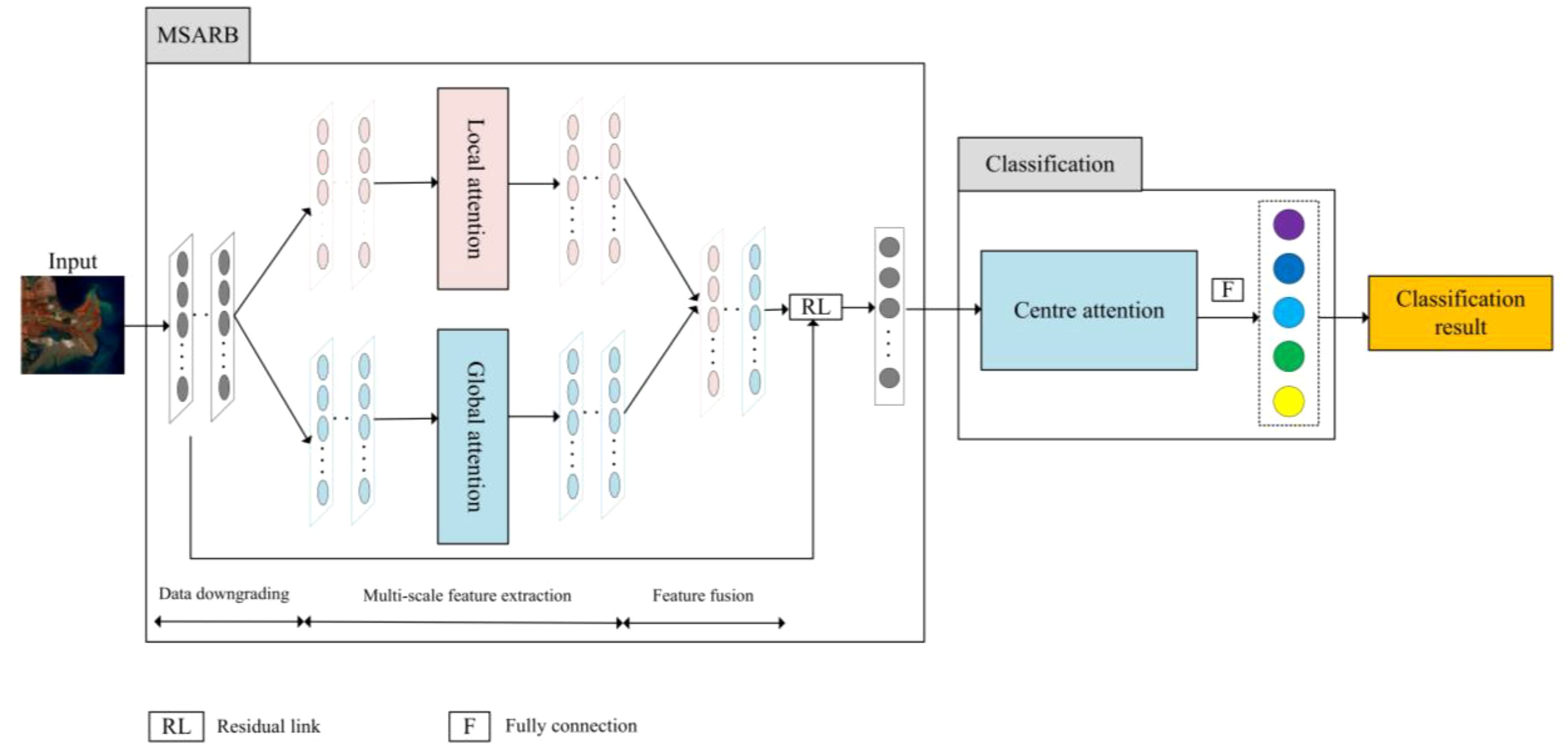
Figure 2. Illustration for influence process of the proposed MARCN.

2.1.1 Reduce the number of channels

The number of channels of the input feature map X is reduced by a convolutional layer with a convolutional kernel of 1 × 1 to minimize the computation and extract preliminary features:

$\begin{array}{ll}X=Con{v}_{new}(x)& (1)\end{array}$

where $Con{v}_{new}$ denotes the new convolution operation for reducing the number of channels.

Convolution operation is an operation to extract features by sliding the convolution kernel over the input feature map and performing the accumulation of dot products. For the input feature map X and convolution kernel K, the convolution operation can be expressed as:

$\begin{array}{ll}Y(i,j)=(K*X)(i,j)=\sum _m\sum _{n}K(m,n)·X(i-m,j-n)& (2)\end{array}$

where $i,j$ denotes the location of the output feature map and $m,n$ traverses the size of the convolution kernel.

2.1.2 Localized attention

The first layer of the attention mechanism is applied to extract 5 × 5 local features. The local attention weights are computed by a convolution operation and a Sigmoid activation function and applied to the feature map:

$\begin{array}{ll}{L}_{att}=\sigma (Con{v}_{local}(x))& (3)\end{array}$

$\begin{array}{ll}{X}_{local}=X\odot L_{att}& (4)\end{array}$

where $Con{v}_{local}$ denotes the convolution operation of local attention, $\sigma$ denotes the Sigmoid activation function, $L_{att}$ is the local attention weight, and $\odot$ denotes element-by-element multiplication.

Element-by-element multiplication is the multiplication of two matrices with elements in the same position, which is useful when applying attention weights

$\begin{array}{ll}(A\odot B)(i,j)=A(i,j)·B(i,j)& (5)\end{array}$

where $A$ and $B$ are two matrices of the same dimension.

2.1.3 Global attention

A second layer of attention is applied to extract 11 × 11 global features. The global attention weights are computed by global averaging of the input feature map, a convolution operation and a Sigmoid activation function and applied to the feature map:

$\begin{array}{ll}{G}_{att}=\sigma (Con{v}_{global}(mean(X,dim=(2,3))))& (6)\end{array}$

$\begin{array}{ll}{X}_{global}=X\odot G_{att}& (7)\end{array}$

where $mean(X,dim=(2,3))$ denotes the global averaging of the dimensionality reduced input feature map X $Con{v}_{global}$ denotes the global attention convolution operation, $\sigma$ denotes the Sigmoid activation function, and $G_{att}$ the global attention weight.

The Sigmoid activation function is used to map the input values between 0 and 1 with the formula:

$\begin{array}{ll}\sigma (x)=\frac{1}{1+e^{-x}}& (8)\end{array}$

It is typically used to generate weights or probability values between 0 and 1.

2.1.4 Feature fusion

Finally, the results of local and global attention are fused to obtain the final feature representation:

$\begin{array}{ll}{X}_{att}=X_{local}+X_{global}& (9)\end{array}$

where, $X_{att}$ denotes the feature map that fuses local and global attention. Convolution operation is performed on $X_{att}$ to obtain the feature map $K$, the features of the middle pixels of $K$ are extracted as the query vector $q$. Matrix multiplication of $K$ and the query vector $q$ is performed to obtain the attention weight $W$:

$\begin{array}{ll}W=softmax\left(\frac{K^T·q}{\sqrt{ck}}\right)& (10)\end{array}$

where $K$ and $q$ are reshape and transpose, respectively, to fit the shape of the matrix multiplication. Compute the weighted feature map $X_1$:

$\begin{array}{ll}{X}_1=\frac{AvgPool(Y\odot W)}{AvgPool(W)}& (11)\end{array}$

where W repeats $C_0$ times to resize $Y$ along the channel direction, $C_0$ is the channel size, $AvgPool$ denotes average pooling, and $\odot$ denotes element-by-element multiplication. Splicing $X_1$ with intermediate pixel features and going through the fully connected layer yields the output $y_0$.

2.2 Reconstructed module

The main function of the spatial information reconstruction module is to enhance the spatial features of the input feature map. Firstly, it checks whether the self-attention is initialized or not, after that, the input feature map X is sampled and reconstructed to construct the query, key and value required by the self-attention mechanism. The self-attention mechanism obtains a weighted feature representation by computing the similarity weighted values between the query and key. This process helps the model to capture the global dependencies in the input feature graph. In addition to the self-attention mechanism, the spatial information reconstruction module processes the input feature map through a convolutional layer, an operation that helps to capture local feature information. Finally, the output of the self-attention mechanism and the output of the convolution operation are weighted and fused using rate1 and rate2 defined during initialization. This preserves both global spatial information and local detail information, thus enhancing the model’s ability to process spatial features. The MSE loss used in RSPAA is defined as:

$\begin{array}{ll}{ℒ}_{RSPAA}={\displaystyle \sum _{b=1}^B\Vert y^b-p^b{\Vert }_2}& (12)\end{array}$

where $y^b$ is the original pixel, it can be obtained by extracting the value of the center pixel directly from the input feature map X. $p^b$ is the result of RSPAA, it is obtained through pooling and a fully connected layer, and b is the batch size.

The main function of the spectral information reconstruction module is to reconstruct and enhance the input spectral features. As shown in Figure 3, by calculating the number of features selected to retain a certain percentage, an equally spaced index array is generated to select specific features from the input features. This selective feature extraction can reduce the amount of data that the model needs to process, thereby reducing the computational complexity. Attention mechanism is introduced to further process the linearly transformed features. The attention mechanism enables the model to focus on the most important features, assign a weight to each feature by calculating the similarity between the features, and then use these weights to weight the features to obtain a weighted feature representation. The features processed by the attention mechanism are fused with the original linearly transformed features. This step is achieved by a simple addition operation:

Figure 3

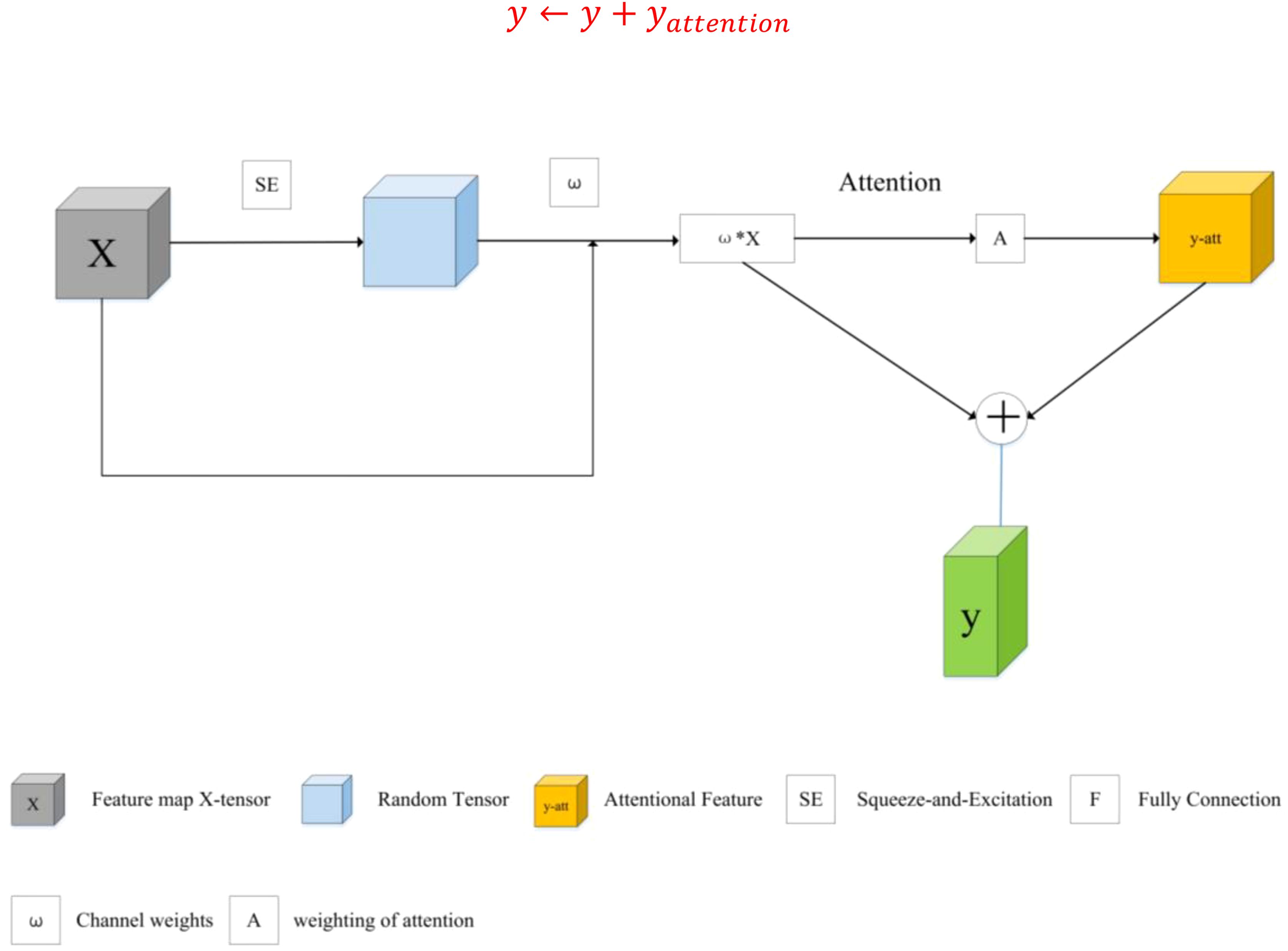
Figure 3. Description of the spectral information reconstruction module.

$\begin{array}{ll}y\leftarrow y+y_{attention}& (13)\end{array}$

This fusion helps to preserve the original features while introducing features enhanced by attentional mechanisms, thus improving the characterization of the features. This process is particularly critical for improving performance in spectral image recognition tasks. The MSE is used as the loss function and the original pixels are used as labels for training. The MSE loss used in RSPEA is defined as:

$\begin{array}{ll}{ℒ}_{RSPEA}={\displaystyle \sum _{b=1}^B\Vert y^b-p^b{\Vert }_2}& (14)\end{array}$

where $y^b$ is the original pixel, it can be obtained by extracting the value of the center pixel directly from the input feature map X. $p^b$ is the result of RSPAA, it is obtained through pooling and a fully connected layer, and b is the batch size.

2.3 Customizing the loss function

The training code mainly uses two loss functions: Cross Entropy Loss and Center Loss, and the loss functions are described in detail below.

2.3.1 Cross entropy loss

In deep learning, the cross-entropy loss function is widely used in multi-category recognition tasks. Assuming that there are N categories, for each sample, we represent its label with an N-dimensional vector, where only one element is 1, indicating the true category of the sample, and the rest of the elements are 0. The output of the model is usually an N-dimensional vector processed by a $softmax$ activation function, which represents the probability that the sample belongs to each category. The cross-entropy loss function is formulated as follows:

$\begin{array}{ll}{ℒ}_{CE}=-{\displaystyle \sum _{c=1}^M{y}_{oc}\log (p_{oc})}& (15)\end{array}$

where $M$ is the total number of classes, $y_{oc}$ indicates the true class, and $p_{oc}$ is the predicted probability.

2.3.2 Center loss

The loss function of Center loss consists of two parts: $softmax$ loss and center loss, where the softmax loss is used for the recognition task, and the center loss is used to constrain the distance between the feature vector and the centroid, which is usually calculated by using the Euclidean distance or cosine distance. The purpose is to make the feature vector as close as possible to the centroid of its corresponding category, so as to form a clear category boundary in the feature space and improve the discriminative property of the features, and finally achieve the compactness learning of the features by optimizing the center loss, which in turn improves the recognition performance of the model. The formula of the Center loss function is as follows.

$\begin{array}{ll}{ℒ}_{Center}=\frac{1}{2}{\displaystyle \sum _{i=1}^m\Vert X_i-C_{y_i}{\Vert }_2^2}& (16)\end{array}$

where $X_i$ is the depth feature of sample $i$, $C_{y_i}$ is the center of the category to which sample $i$ belongs, and $m$ is the batch size. center loss promotes intra-class compactness by minimizing the Euclidean distance between a sample feature and its corresponding category center.

In summary, the network’s ultimate loss is.

$\begin{array}{ll}ℒ={ℒ}_{RSPAA}+{ℒ}_{RSPEA}+{ℒ}_{CE}+\lambda {ℒ}_{Center}& (17)\end{array}$

where $\lambda$ is a weight parameter used to balance the two losses. This combination exploits the effectiveness of the cross-entropy loss in the recognition task, but also enhances the differentiation of the features through the Center loss, thus improving the performance of the model.

3 Experimentation and analysis

In this section, the Yellow River Estuary (YRE) and the Gaofeng State Owned Forest Farm (GSOFF) hyperspectral datasets are used to evaluate the effectiveness of the proposed MARCN. The GSOFF dataset, as an extended dataset, is used to verify the generalization ability of this algorithm. First, the YRE and the GSOFF datasets are introduced, second, ablation experiments are conducted to verify the effectiveness of MARCN, and finally, several state-of-the-art conventional algorithms are used to compare with the proposed MARCN algorithm to verify the efficiency of the proposed algorithm MARCN.

3.1 Data sets

(1) Yellow River Estuary: The dataset was collected by GF-5 satellite over the Yellow River Delta in November 2018, with a data size of 1,185 × 1,342 pixels. The spatial resolution of images is 30m. The images have a spectral resolution of 5 nm, 150 spectral bands in the VNIR 0.40 ~ 1.00 µm range, 180 spectral bands in the SWIR wavelength range of 1.00 ~ 2.50 µm, and a spectral resolution of 10 nm.1-2 near-infrared (NIR) bands, as well as 175-180, 172-173, 119-121, 96-115, and 42- 53 SWIR bands were shifted, leaving a total of 285 bands. It has 20 wetland bands. Table 1 shows the number of training and test samples. The pseudo-color and sample distribution maps are shown in Figure 4.

Table 1

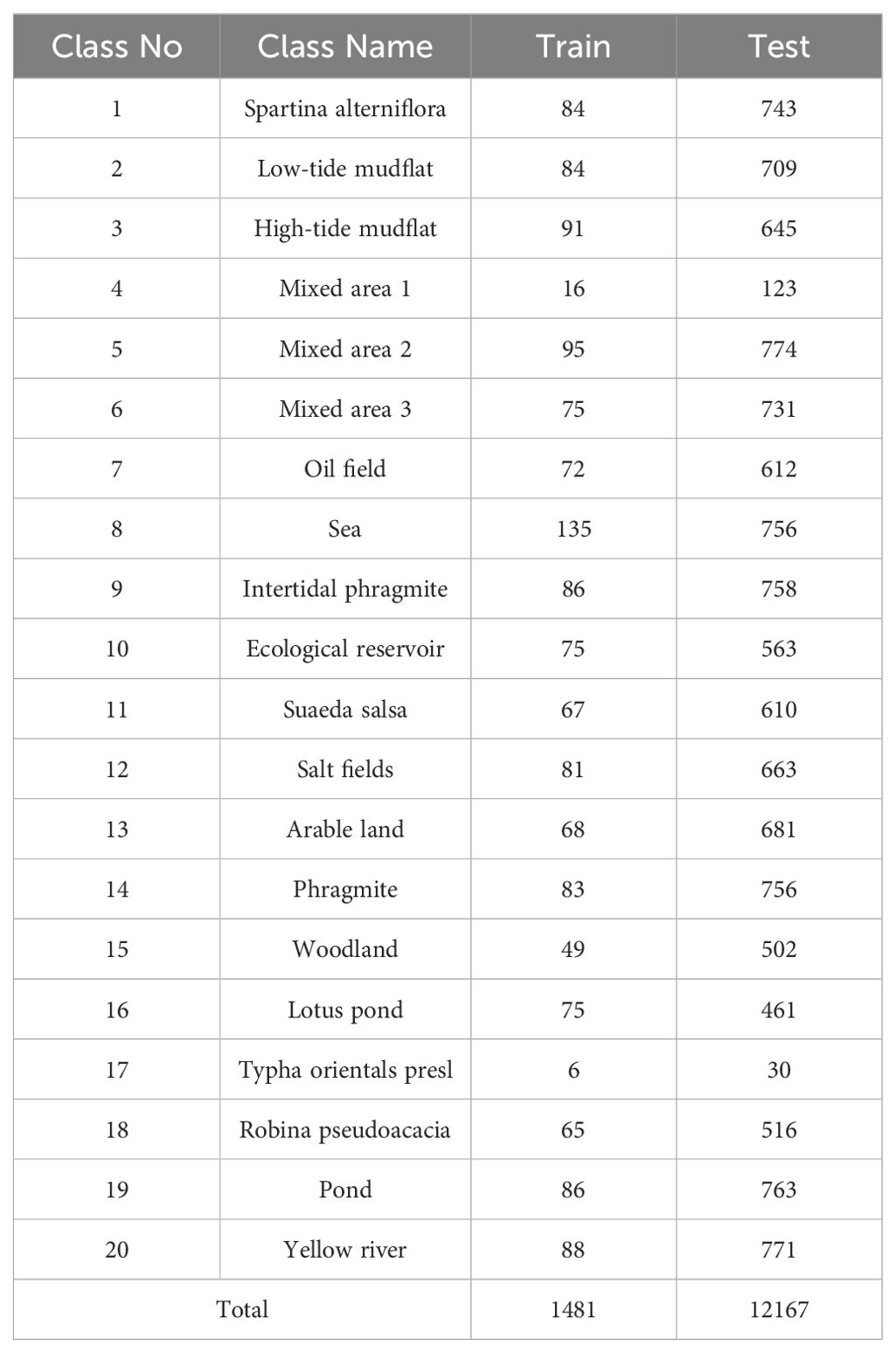
Table 1. Class labels and train-test samples distribution of YRE.

Figure 4

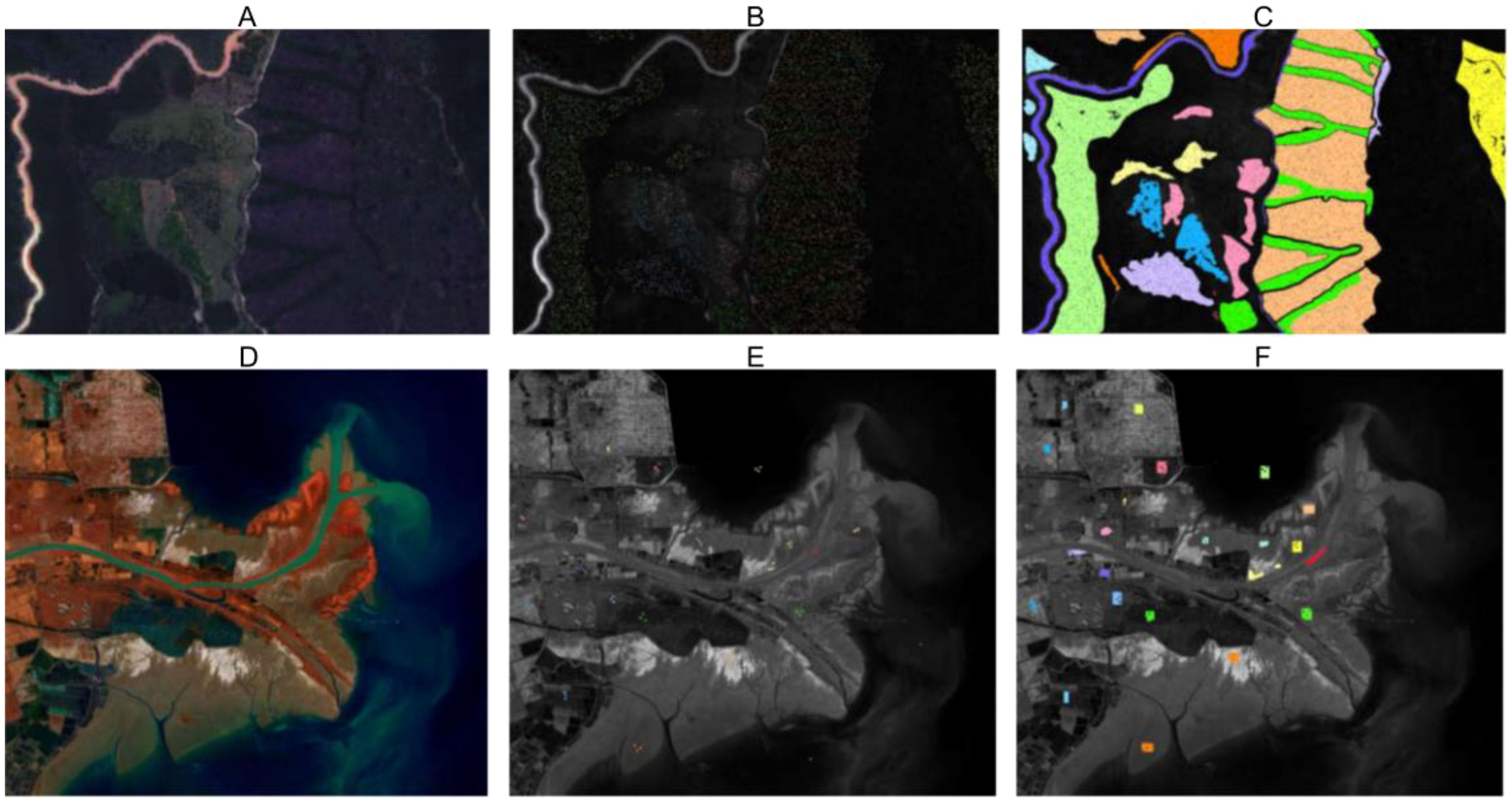
Figure 4. Maps of false color and training and testing samples distributions of GSOFF and YRE datasets, respectively. For the GSOFF dataset (A–C) are pseudo color images, training set, and testing set, respectively. For the YRE dataset, (D–F) are pseudo color images, training set, and testing set, respectively.

(2) Gaofeng State Owned Forest Farm: In January 2018, the GSOFF dataset was acquired using the AISA Eagle II diffraction grating push-broom hyperspectral imager over the Gaofeng State-Owned Forest Farm in Guangxi, China. This dataset features a spatial resolution of 1m×1m and a spectral resolution of 3.3nm, encompassing an image size of 572×906 pixels. The hyperspectral data comprises 125 spectral bands spanning wavelengths from 0.4 to 1.0 µm. It includes nine different forest vegetation categories and three additional categories. Table 2 details the number of training and test samples, while Figure 4 presents the pseudo-color and sample distribution maps.

Table 2

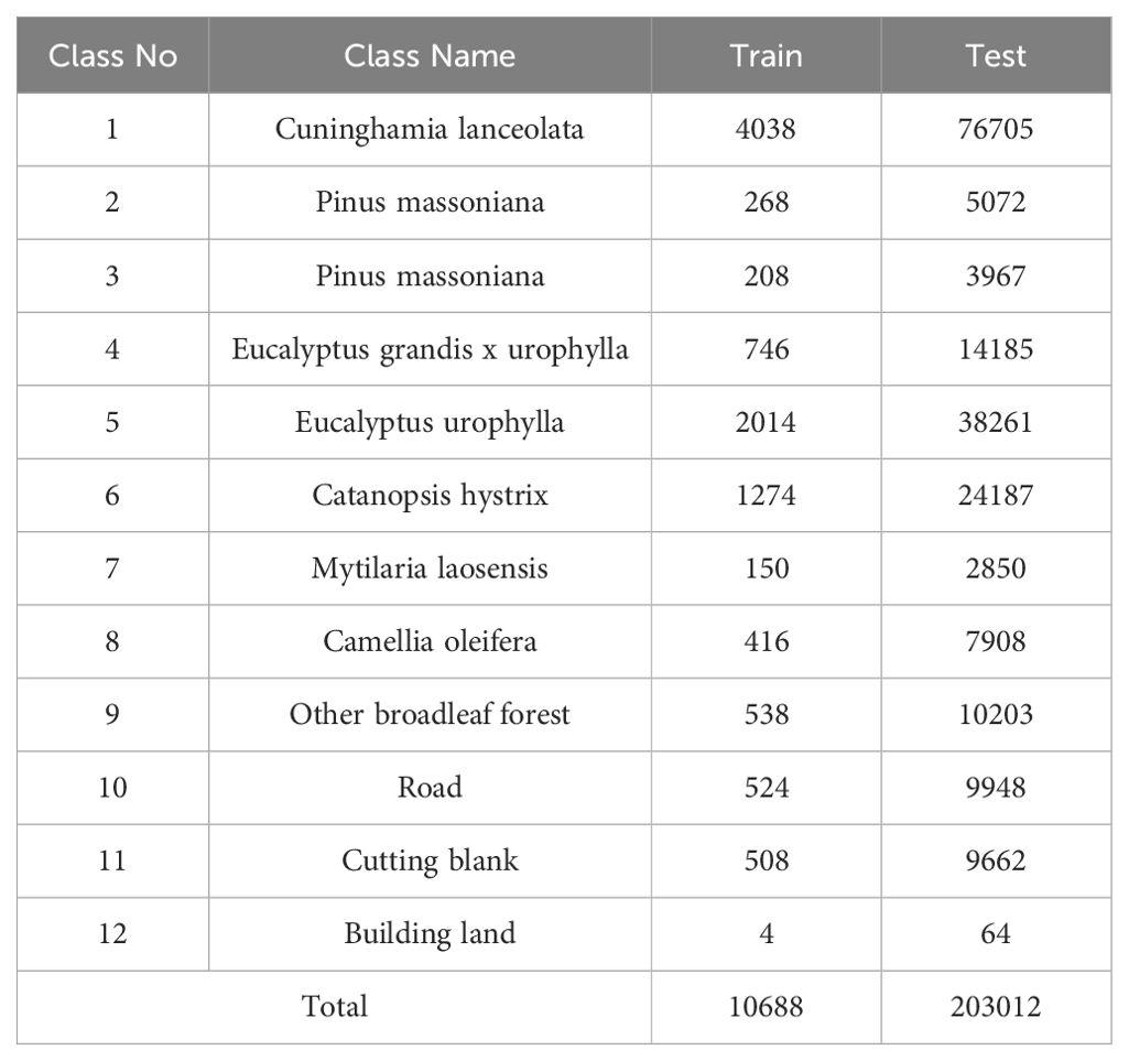
Table 2. Class labels and train-test samples distribution of GSOFF.

3.2 Ablation studies

The purpose of the ablation experiments is to validate the feature extraction module, reconstruction module, and loss function of the proposed MARCN. The recognition performance is measured using OA (Overall Accuracy). As shown in Table 3, there is a significant improvement in the recognition accuracy after adding RSPAA and RSPEA to HIS recognition. In MARCN, for the datasets YRE, the OA increased by 1.82%. To verify the algorithm’s strong generalization capabilities, we conducted an extended validation on the GSOFF datasets, achieving a 0.49% increase in accuracy. Thus, the effectiveness of RSPAA and RSPEA for hyperspectral image recognition is confirmed.

Table 3

Table 3. Analysis experiments about the suggested RESPA, RESPE, MSA, and CL in reference to the classification performance (overall accuracy [%]) for YRE and GSOFF datasets.

In order to validate the effectiveness of the proposed multi-scale attention feature extraction module, experiments are conducted with the conventional convolutional MrCNN instead of the MARCN module. From the experimental results, it can be seen that OA increases by 5.56% on the datasets YRE. To test the algorithm’s generalization, we performed an extended validation on the GSOFF datasets, resulting in a 6.83% increase in accuracy. Therefore, the effectiveness of multi-scale attention feature extraction is verified.

As shown in Table 3, there is a significant improvement in the recognition performance after adding Center loss (CL) to hyperspectral image recognition. In MARCN, the OA of YRE and GSOFF datasets increased by 4.07% and 0.43% respectively. Therefore, the effectiveness of Center loss for HSI recognition is confirmed.

3.3 Parametric analysis

The core parameters of MARCN are RA and RE, which represent the mask ratios of RSPAA and RSPEA, respectively, and by adjusting the ratio, the complexity and computational power of the model can be controlled. Lower values of ratio mean that more features are retained, which may increase the computational burden of the model, but may also improve the model’s ability to capture details. Higher values of ratio, on the other hand, reduce the number of features and may help reduce overfitting and improve the model’s ability to generalize. Choose from 0.25, 0.5, 0.75, 0.85, and 0.9g. In Tables 4 and 5, it can be seen that as the ratio increases, the change in recognition accuracy is not very significant, indicating that the network model already has good robustness.

Table 4

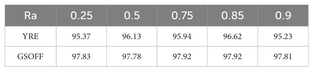
Table 4. Analysis experiments about the parameter Ra in reference to the classification performance (overall accuracy [%]) for YRE and GSOFF datasets.

Table 5

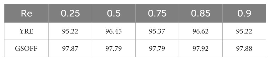
Table 5. Analysis experiments about the parameter Re in reference to the classification performance (overall accuracy [%]) for YRE and GSOFF datasets.

3.4 Comparison algorithm analysis

The proposed method’s detection performance was validated using nine hyperspectral classification methods for comparison. These methods include CNNHSI (Hu et al., 2015), RPCACNN (Makantasis et al., 2015), OTVCA (Rasti et al., 2016), SSCNN (Mei et al., 2017), CDCNN (Lee and Kwon, 2017), DRCNN (Zhang et al., 2018), FusCNNGCN (He et al., 2019), 3DCNN (Zhang et al., 2020), and BERTHSI (Hong et al., 2020). The parameters for these nine methods were set according to the original publications to optimize their performance.

In Tables 6 and 7, the recognition performance is evaluated using class-specific accuracy (CA), overall accuracy (OA), average accuracy (AA), and the Kappa coefficient. The RPCACNN method shows poor performance on both datasets, likely because it loses some discriminative information during RPCA-based dimensionality reduction, especially when noise reduction or outlier removal is emphasized. Methods like SSCNN (Mei et al., 2017), CDCNN (Lee and Kwon, 2017), DRCNN (Zhang et al., 2018), and 3DCNN (Zhang et al., 2020) fail to capture global dependencies between pixel points, leading to insufficient comprehension of the overall semantic information, thereby affecting recognition performance. Hyperspectral images contain both spatial and spectral information, making it crucial to fuse these two types of information effectively. However, algorithms such as OTVCA (Rasti et al., 2016), CNNHSI (Hu et al., 2015), FusCNNGCN (He et al., 2019), and 3DCNN (Zhang et al., 2020) are inadequate in spatial-spectral information fusion, resulting in the underutilization of spectral and spatial information. The MARCN proposed in this study demonstrates the best recognition performance on both datasets, with OA improvements of 1.33% and 4.06% over the second-highest method.

Table 6

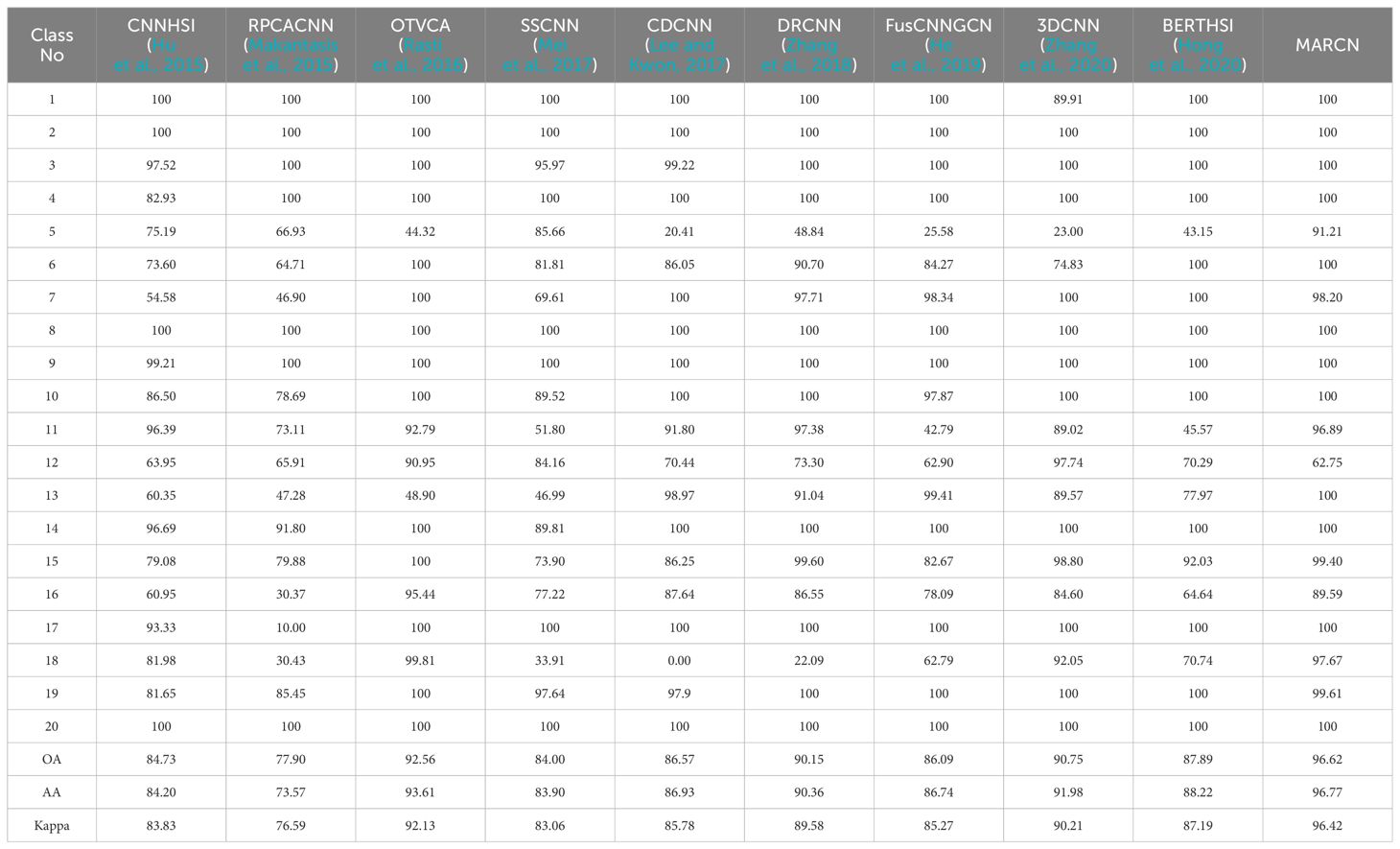
Table 6. Classification results [%] of YRE with different methods.

Table 7

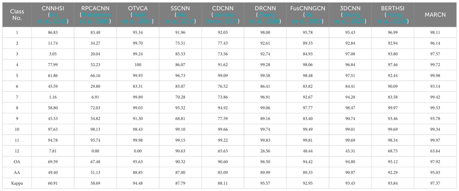
Table 7. Classification results [%] of GSOFF with different methods.

Figures 5 and 6 demonstrates the recognition effect of all the methods, from which it can be seen that among the baseline methods, the RPCACNN has the worst recognition effect graph, recognizing the salt field as a mudflat, and the lotus pond fails to be recognized. OTVCA, DRCNN and 3DCNN recognize relatively well, however, the OTVCA algorithm generates results that are too smooth and the detail information is submerged, which is because local features in the data are not well captured, resulting in data loss. Methods such as DRCNN and 3DCNN ignore the global dependencies between pixel points, leading to insufficient understanding of the overall semantic information in the model and affecting the recognition effect. CNNHSI and FusCNNGNN contain more noise points in their recognition results. Compared to the baseline methods, the MARCN algorithm proposed in this study achieves higher recognition accuracy with fewer mislabeled pixels. The observed smoothness and distinct boundary features in the results are due to the introduction of the spectral information reconstruction module and the spatial information reconstruction module. These modules enhance the utilization of spectral and spatial features, effectively reduce noise interference, accurately detect object boundaries, and preserve image details.

Figure 5

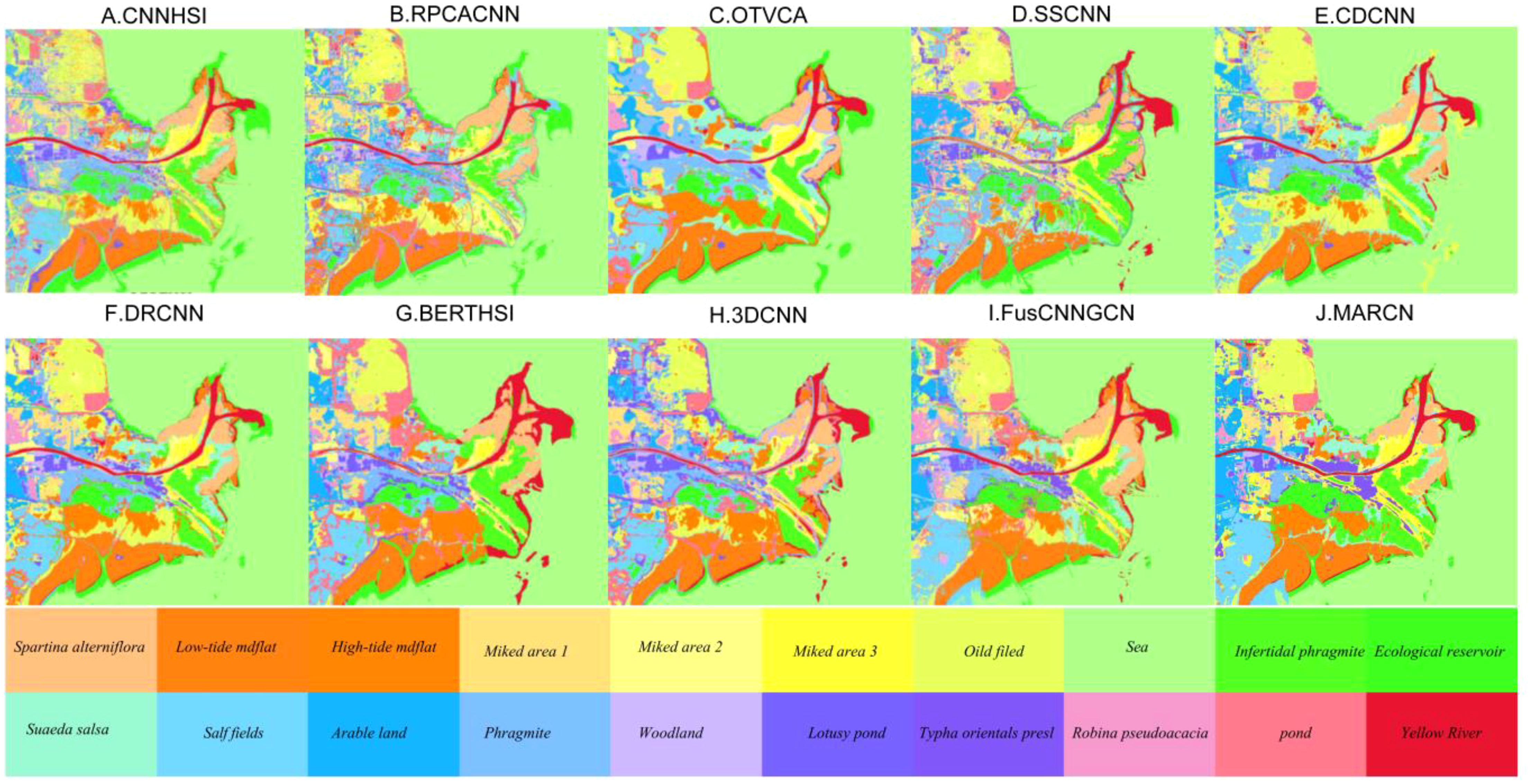
Figure 5. YRE’s classification maps of different methods. (A) is the classification result of the CNNHSI algorithm, (B) is the classification result of the RPCACNN algorithm, (C) is the classification result of the OTVCA algorithm, (D) is the classification result of the SSCNN algorithm, (E) is the classification result of the CDCNN algorithm, (F) is the classification result of the DRCNN algorithm, (G) is the classification result of the BERTHSI algorithm, (H) is the classification result of the 3DCNN algorithm, (I) is the classification result of the FusCNNGCN algorithm, and (J) is the classification result of the MARCN algorithm.

Figure 6

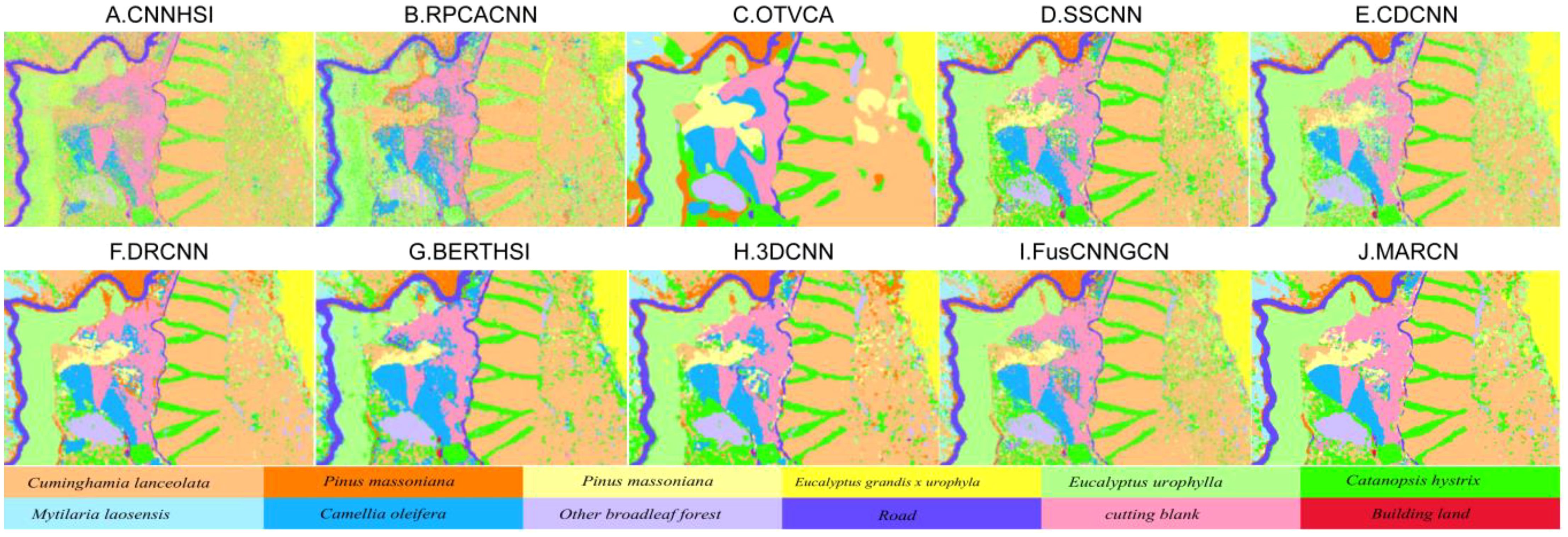
Figure 6. GSOFF’s classification maps of different methods. (A) is the classification result of the CNNHSI algorithm, (B) is the classification result of the RPCACNN algorithm, (C) is the classification result of the OTVCA algorithm, (D) is the classification result of the SSCNN algorithm, (E) is the classification result of the CDCNN algorithm, (F) is the classification result of the DRCNN algorithm, (G) is the classification result of the BERTHSI algorithm, (H) is the classification result of the 3DCNN algorithm, (I) is the classification result of the FusCNNGCN algorithm, and (J) is the classification result of the MARCN algorithm.

4 Conclusion

In nearshore scenarios, the MARCN method successfully addresses the limitations of traditional feature extraction methods in complex environments through its multiscale attention mechanism and reconstruction modules. The introduction of the center loss function effectively reduces intra-class differences, making spectral features of different types more concentrated and easier to distinguish. This improves the accuracy and robustness of recognition. In experiments, MARCN outperformed existing hyperspectral feature extraction methods in nearshore environments, showing significant advantages in complex and variable conditions. However, MARCN has certain limitations, such as dependency on specific types of data and the need for substantial computational resources. Future work can focus on optimizing the algorithm’s computational efficiency and further enhancing its recognition capabilities in extreme environments.

Overall, the application of MARCN in nearshore scenarios demonstrates its significant potential in environmental monitoring, resource management, and disaster warning. By effectively extracting and processing complex spectral-spatial information, MARCN excels in diverse and changing environmental conditions.

Data availability statement

The original contributions presented in the study are included in the article/supplementary material. Further inquiries can be directed to the corresponding authors.

Author contributions

SZ: Conceptualization, Methodology, Writing – review & editing. LW: Data curation, Validation, Writing – original draft. LS: Writing – review & editing. PM: Writing – review & editing. LL: Writing – review & editing. ZL: Supervision, Writing – review & editing. XZ: Writing – review & editing.

Funding

The author(s) declare financial support was received for the research, authorship, and/or publication of this article. This work was supported in part by the Scientific and Technological Project in Henan Province [grant number 232102320258]; The Open Fund Projects of Henan Key Laboratory of General Aviation Technology [grant number ZHKF-230211]; National Natural Science Foundation of China [grant number 42174037]; Henan Center for Outstanding Overseas Scientists [grant number GZS2020012]; the Fund of Henan Province Collaborative Innovation Center of Aeronautics and Astronautics Electronic Information Technology; and was partly supported by the Open Project of Tianjin Key Laboratory of Autonomous Intelligence Technology and Systems No. AITS-20240001.

Acknowledgments

All authors would like to thank the reviewer for their valuable suggestions on this paper. We also appreciate the assistance provided by all researchers involved in this study. Additionally, we are grateful to the researchers who provided comparative methods.

Conflict of interest

The authors declare that the research was conducted in the absence of any commercial or financial relationships that could be construed as a potential conflict of interest.

Publisher’s note

All claims expressed in this article are solely those of the authors and do not necessarily represent those of their affiliated organizations, or those of the publisher, the editors and the reviewers. Any product that may be evaluated in this article, or claim that may be made by its manufacturer, is not guaranteed or endorsed by the publisher.

References

Arshad T., Zhang J. (2024). Hierarchical attention transformer for hyperspectral image classification. IEEE Geosci. Remote Sens. Lett. 21, 1–5. doi: 10.1109/LGRS.2024.3379509

Crossref Full Text | Google Scholar

Chang C. I., Lin C. Y., Chung P. C., Hu P. F. (2023). Iterative spectral–spatial hyperspectral anomaly detection. IEEE Trans. Geosci. Remote Sens. 61, 1–30. doi: 10.1109/TGRS.2023.3247660

Crossref Full Text | Google Scholar

Chen L., Liu J., Sun S., Chen W., Du B., Liu R. (2023). An iterative GLRT for hyperspectral target detection based on spectral similarity and spatial connectivity characteristics. IEEE Trans. Geosci. Remote Sens. 61, 1–11. doi: 10.1109/TGRS.2023.3252052

Crossref Full Text | Google Scholar

Cheng X., Xu Y., Zhang J., Zeng D. (2022). Hyperspectral anomaly detection via low-rank decomposition and morphological filtering. IEEE Geosci. Remote Sens. Lett. 19, 1–5. doi: 10.1109/LGRS.2021.3126902

Crossref Full Text | Google Scholar

Dosovitskiy A., Beyer L., Kolesnikov A., Weissenborn D., Zhai X., Unterthiner T., et al. (2020). An image is worth 16x16 words: Transformers for image recognition at scale. Int. Conf. Learn. Represent. 19 (2s), 1–31. doi: 10.48550/arXiv.2010.11929

Crossref Full Text | Google Scholar

Duan Y., Huang H., Li Z., Tang Y. (2020b). Local manifold-based sparse discriminant learning for feature extraction of hyperspectral image. IEEE Trans. Cybernet. 51, 4021–4034. doi: 10.1109/TCYB.2020.2977461

Crossref Full Text | Google Scholar

Duan Y., Huang H., Tang Y. (2020a). Local constraint-based sparse manifold hypergraph learning for dimensionality reduction of hyperspectral image. IEEE Trans. Geosci. Remote Sens. 59, 613–628. doi: 10.1109/TGRS.2020.2995709

Crossref Full Text | Google Scholar

Gao H., Sheng R., Chen Z., Liu H., Xu S., Zhang B. (2024). Multi-scale random-shape convolution and adaptive graph convolution fusion network for hyperspectral image classification. IEEE Trans. Geosci. Remote Sens. 62, 1–17. doi: 10.1109/TGRS.2024.3390928

Crossref Full Text | Google Scholar

Gao L., Wang D., Zhuang L., Sun X., Huang M., Plaza A. (2023a). BS 3 LNet: A new blind-spot self-supervised learning network for hyperspectral anomaly detection. IEEE Trans. Geosci. Remote Sens. 61, 1–18. doi: 10.1109/TGRS.2023.3246565

Crossref Full Text | Google Scholar

Gao Y., Zhang M., Li W., Song X., Jiang X., Ma Y. (2023b). Adversarial complementary learning for multisource remote sensing classification. IEEE Trans. Geosci. Remote Sens. 61, 1–13. doi: 10.1109/TGRS.2023.3255880

Crossref Full Text | Google Scholar

Gao Y., Zhang M., Wang J., Li W. (2023c). Cross-scale mixing attention for multisource remote sensing data fusion and classification. IEEE Trans. Geosci. Remote Sens. 61, 1–15. doi: 10.1109/TGRS.2023.3263362

Crossref Full Text | Google Scholar

He X., Chen Y. (2019). Optimized input for CNN-based hyperspectral image classification using spatial transformer network. IEEE Geosci. Remote Sens. Lett. 16, 1884–1888. doi: 10.1109/LGRS.2019.2911322

Crossref Full Text | Google Scholar

He J., Zhao L., Yang H., Zhang M., Li W. (2019). HSI-BERT: hyperspectral image classification using the bidirectional encoder representation from transformers. IEEE Trans. Geosci. Remote Sens. 58, 165–178. doi: 10.1109/TGRS.2019.2934760

Crossref Full Text | Google Scholar

Hong D., Gao L., Yao J., Zhang B., Plaza A., Chanussot J. (2020). Graph convolutional networks for hyperspectral image classification. IEEE Trans. Geosci. Remote Sens. 59, 5966–5978. doi: 10.1109/TGRS.2020.3015157

Crossref Full Text | Google Scholar

Hu W., Huang Y., Wei L., Zhang F., Li H. (2015). Deep convolutional neural networks for hyperspectral image classification. J. Sensors 2015, 258619. doi: 10.1155/2015/258619

Crossref Full Text | Google Scholar

Jin Y., Ye M., Xiong F., Qian Y. (2023). “Cross-domain heterogeneous hyperspectral image classification based on meta-learning with task-adaptive loss function,” in 2023 13th Workshop on Hyperspectral Imaging and Signal Processing: Evolution in Remote Sensing (WHISPERS), Athens, Greece. New York, NY, USA: IEEE. 1–5. doi: 10.1109/WHISPERS61460.2023.10430600

Crossref Full Text | Google Scholar

Lee H., Kwon H. (2017). Going deeper with contextual CNN for hyperspectral image classification. IEEE Trans. Image Process. 26, 4843–4855. doi: 10.1109/TIP.2017.2725580

PubMed Abstract | Crossref Full Text | Google Scholar

Li J., Wong Y., Zhao Q., Kankanhalli M. S. (2019). “Learning to learn from noisy labeled data,” in 2019 IEEE/CVF Conference on Computer Vision and Pattern Recognition (CVPR), Long Beach, CA, USA. New York, NY, USA: IEEE. 5046–5054. doi: 10.1109/CVPR.2019.00519

Crossref Full Text | Google Scholar

Li T., Zhang X., Zhang S., Wang L. (2022). Self-supervised learning with a dual-branch resNet for hyperspectral image classification. IEEE Geosci. Remote Sens. Lett. 19, 1–5. doi: 10.1109/LGRS.2021.3107321

Crossref Full Text | Google Scholar

Lin T. Y., Goyal P., Girshick R., He K., Dollár P. (2017). Focal loss for dense object detection. IEEE Trans. Pattern Anal. Mach. Intell. 42, 318–327. doi: 10.1109/TPAMI.2018.2858826

Crossref Full Text | Google Scholar

Liu R., Lei C., Xie L., Qin X. (2024). A novel endmember bundle extraction framework for capturing endmember variability by dynamic optimization. IEEE Trans. Geosci. Remote Sens. 62, 1–17. doi: 10.1109/TGRS.2024.3354046

Crossref Full Text | Google Scholar

Liu C., Li J., He L., Plaza A., Li S., Li B. (2020). Naive gabor networks for hyperspectral image classification. IEEE Trans. Neural Networks Learn. Syst. 32, 376–390. doi: 10.1109/TNNLS.2020.2978760

Crossref Full Text | Google Scholar

Makantasis K., Karantzalos K., Doulamis A., Doulamis N. (2015). “Deep supervised learning for hyperspectral data classification through convolutional neural networks,” in 2015 IEEE International Geoscience and Remote Sensing Symposium (IGARSS), Milan, Italy. New York, NY, USA: IEEE. 4959–4962. doi: 10.1109/IGARSS.2015.7326945

Crossref Full Text | Google Scholar

Mei S., Ji J., Hou J., Li X., Du Q. (2017). “Learning sensor-specific features for hyperspectral images via 3-dimensional convolutional autoencoder,” in 2017 IEEE International Geoscience and Remote Sensing Symposium (IGARSS), Fort Worth, TX, USA. New York, NY, USA: IEEE. 1820–1823. doi: 10.1109/IGARSS.2017.8127329

Crossref Full Text | Google Scholar

Niu Z., Liu W., Zhao J., Jiang G. (2018). DeepLab-based spatial feature extraction for hyperspectral image classification. IEEE Geosci. Remote Sens. Lett. 16, 251–255. doi: 10.1109/LGRS.2018.2871507

Crossref Full Text | Google Scholar

Peng J., Li L., Tang Y. Y. (2018). Maximum likelihood estimation-based joint sparse representation for the classification of hyperspectral remote sensing images. IEEE Trans. Neural Networks Learn. Syst. 30, 1790–1802. doi: 10.1109/TNNLS.2018.2874432

Crossref Full Text | Google Scholar

Rasti B., Ulfarsson M. O., Sveinsson J. R. (2016). Hyperspectral feature extraction using total variation component analysis. IEEE Trans. Geosci. Remote Sens. 54, 6976–6985. doi: 10.1109/TGRS.2016.2593463

Crossref Full Text | Google Scholar

Schroff F., Kalenichenko D., Philbin J. (2015). “FaceNet: A unified embedding for face recognition and clustering,” in 2015 IEEE Conference on Computer Vision and Pattern Recognition (CVPR), Boston, MA, USA. New York, NY, USA: IEEE. 815–823. doi: 10.1109/CVPR.2015.7298682

Crossref Full Text | Google Scholar

Shen X., Yu H., Yu C., Wang Y., Song M. (2021). “Global spatial and local spectral similarity based sample augment and extended subspace projection for hyperspectral image classification,” in 2021 IEEE International Geoscience and Remote Sensing Symposium IGARSS, Brussels, Belgium. New York, NY, USA: IEEE. 3637–3640. doi: 10.1109/IGARSS47720.2021.9554113

Crossref Full Text | Google Scholar

Tan X., Zhao Z., Xu X., Li S. (2024). “Multi-scale diffusion features fusion network for hyperspectral image classification,” in 2024 4th Asia Conference on Information Engineering (ACIE), Singapore, Singapore. New York, NY, USA: IEEE. 65–73. doi: 10.1109/ACIE61839.2024.00018

Crossref Full Text | Google Scholar

Vaswani A., Shazeer N., Parmar N., Uszkoreit J., Jones L., Gomez A. N., et al. (2017). Attention is all you need. Adv. Neural Inf. Process. Syst. 30, 5998–6008. doi: 10.48550/arXiv.1706.03762

Crossref Full Text | Google Scholar

Xiaoxia Z., Xia Z. (2024). Attention-based deep convolutional capsule network for hyperspectral image classification. IEEE Access 12, 56815–56823. doi: 10.1109/ACCESS.2024.3390558

Crossref Full Text | Google Scholar

Xie J., Fang L., Zhang B., Chanussot J., Li S. (2021). Super resolution guided deep network for land cover classification from remote sensing images. IEEE Trans. Geosci. Remote Sens. 60, 1–12. doi: 10.1109/TGRS.2021.3120891

Crossref Full Text | Google Scholar

Yang H., Yu H., Hong D., Xu Z., Wang Y., Song M. (2022). “Hyperspectral image classification based on multi-level spectral-spatial transformer network,” in 2022 12th Workshop on Hyperspectral Imaging and Signal Processing: Evolution in Remote Sensing (WHISPERS), Rome, Italy. New York, NY, USA: IEEE. 1–4. doi: 10.1109/WHISPERS56178.2022.9955116

Crossref Full Text | Google Scholar

Yu H., Yang H., Gao L., Hu J., Plaza A., Zhang B. (2024). Hyperspectral image change detection based on gated spectral–spatial–temporal attention network with spectral similarity filtering. IEEE Trans. Geosci. Remote Sens. 62, 1–13. doi: 10.1109/TGRS.2024.3373820

Crossref Full Text | Google Scholar

Yue J., Fang L., Rahmani H., Ghamisi P. (2021). Self-supervised learning with adaptive distillation for hyperspectral image classification. IEEE Trans. Geosci. Remote Sens. 60, 1–13. doi: 10.1109/TGRS.2021.3057768

Crossref Full Text | Google Scholar

Zhang M., Li W., Du Q. (2018). Diverse region-based CNN for hyperspectral image classification. IEEE Trans. Image Process. 27, 2623–2634. doi: 10.1109/TIP.2018.2809606

PubMed Abstract | Crossref Full Text | Google Scholar

Zhang X., Li W., Gao C., Yang Y., Chang K. (2023). Hyperspectral pathology image classification using dimensiondriven multi-path attention residual network. Expert Syst. Appl. 230, 120615. doi: 10.1016/j.eswa.2023.120615

Crossref Full Text | Google Scholar

Zhang W., Su L., Zhang Y., Lu X. (2023). A spectrum-aware transformer network for change detection in hyperspectral imagery. IEEE Trans. Geosci. Remote Sens. 61, 1–12. doi: 10.1109/TGRS.2023.3299642

Crossref Full Text | Google Scholar

Zhang J., Zhao R., Shi Z., Zhang N., Zhu X. (2021). Bayesian constrained energy minimization for hyperspectral target detection. IEEE J. Select. Topics Appl. Earth Observ. Remote Sens. 14, 8359–8837. doi: 10.1109/JSTARS.2021.3104908

Crossref Full Text | Google Scholar

Zhang B., Zhao L., Zhang X. (2020). Three-dimensional convolutional neural network model for tree species classification using airborne hyperspectral images. Remote Sens. Environ. 247, 111938. doi: 10.1016/j.rse.2020.111938

Crossref Full Text | Google Scholar

Zhao X., Liu K., Gao K., Li W. (2023). Hyperspectral time-series target detection based on spectral perception and spatial–temporal tensor decomposition. IEEE Trans. Geosci. Remote Sens. 61, 1–12. doi: 10.1109/TGRS.2023.3307071

Crossref Full Text | Google Scholar

Zhao J., Wang G., Zhou B., Ying J., Liu J. (2023). SRA–CEM: an improved CEM target detection algorithm for hyperspectral images based on subregion analysis. IEEE J. Select. Topics Appl. Earth Observ. Remote Sens. 16, 6026–6037. doi: 10.1109/JSTARS.2023.3289943

Crossref Full Text | Google Scholar

Zheng K., Gao L., Zhang B., Cui X. (2018). “Multi-losses function based convolution neural network for single hyperspectral image super-resolution,” in 2018 Fifth International Workshop on Earth Observation and Remote Sensing Applications (EORSA), Xi’an, China. New York, NY, USA: IEEE. 1–4. doi: 10.1109/EORSA.2018.8598551

Crossref Full Text | Google Scholar