Numerical investigation for the influence of suspended sediment on salinity distribution in the Qiantang Estuary, China

Numerous studies have demonstrated that high suspended sediment concentration (SSC) can change density distribution and affect water mixing, but few scholars have investigated this impact on numerical simulations of estuarian salinity distribution. The Qiantang Estuary is a macro-tidal estuary with high SSC, which has a more significant influence on water density than that of salinity. Therefore, this paper established a three-dimensional (3D) numerical model coupling flow, salinity and SSC based on Delft3D and first analyzes the impact of SSC on salinity distribution under different runoff and tidal conditions in the Qiantang Estuary. The results indicated that simulated salinity generally decreases when considering the impact of SSC, suggesting a weakening effect on saltwater intrusion. The distribution of salinity difference (ΔS) and SSC show a strong spatial and temporal correlation, and ΔS peak increases and shifts upstream as the tidal range increases or runoff discharge decreases. The mechanism of SSC influencing saltwater intrusion can be summarized as follows: On the one hand, SSC increases the water density, which weakens the driving force for saltwater to move upstream, causing a decrease in flood current velocity and water level, and thereby diminishing the advective transport of salinity. On the other hand, SSC enhances density stratification, which weakens vertical turbulence and reduces the dispersive transport of salinity. These combined effects reduce both the advective and diffusive salinity fluxes during the flood tide, ultimately leading to a decrease in upstream salinity. Therefore, neglecting this effect in estuaries with high SSC can cause significant deviations in salinity simulation results, especially under low-flow and high-tide conditions.

1 Introduction

As a marker of freshwater mixing, salinity is an important indicator of freshwater mixing and material exchanges in the estuary (Guillou et al., 2023). The spatial and temporal distribution of salinity plays an important role in water resource utilization (Bellafiore et al., 2021; Bricheno et al., 2021; Wu et al., 2023), sediment transport (Shen et al., 2020; Zhu et al., 2021) and estuarine ecosystem (Telesh and Khlebovich, 2010; Weng et al., 2020; Moseev et al., 2022). However, the distribution of estuarine salinity is influenced by various factors, including runoff and tides, wind, river topography, sea level rise, and human activities (Jiao et al., 2021; Wu et al., 2023; Gao et al., 2024). Therefore, it is of great significance to study the influence of these factors on salinity distribution for a more accurate simulation of salinity in the estuary.

With the advancement of computer technology, numerical models based on physical processes have been widely used for salinity simulations in the estuary (Hu et al., 2019). There have been various numerical simulation studies on the factors affecting estuarine salinity distribution. Chen et al. (2016) established a three-dimensional (3D) model to study the responses of estuarine salinity distribution and transport processes to sea level rise in the Zhujiang (Pearl River) Estuary. Akter and Tanim (2021) investigated the response of salinity distribution and stratification to tidal circulation, seasonal variation, topography and river discharge in the Karnafuli River Estuary by a subgrid-scale Horizontal Large Eddy Simulation model in Delft3D. Álvarez et al. (2022)studied the impact of wave effects on salinity distribution in the Magdalena River Estuary based on field measurements and the MOHID 3D model system. Based on FVCOM numerical modeling, Shi et al. (2020) and Qin et al. (2023) investigated the influence of river discharge on salinity distribution and diffusion of the Yellow River Estuary and Laizhou Bay. Zhao et al. (2022) applied a process-based hydrodynamic model (Delft3D) to investigate the salinity distributions and variations in the Yangtze Estuary and studied the combined effects of river discharge regulation and estuarine morphological evolution on salinity dynamics. However, these models primarily focus on the effect of hydrodynamic-related factors (such as runoff, tides, wind, etc.) on salinity distribution, neglecting the impact of suspended sediment concentration (SSC) on water density. Currently, very few studies have incorporated the effect of SSC in estuarine salinity simulation.

The high SSC not only leads to a significant increase in the water density, but also changes the vertical density gradient and causes stratification in the estuary, which affects the turbulence structure and water mixing (Lu et al., 2020). This phenomenon has been confirmed in many field observations and numerical simulations. Winterwerp (2001, 2006) conducted a concise literature review and numerical experiments and found that the stratification effects by cohesive and noncohesive sediment may cause an appreciable modification of the vertical profiles of velocity, vertical eddy viscosity/diffusivity, and Reynolds stresses. Jones and Monismith (2008) found that the dissipation measurements were either equal to or less than that predicted by wall-layer theory due to stratification induced by the SSC gradients near the bed in the shallow embayment of Grizzly Bay, San Francisco Bay, California. Wan and Wang (2017) used Delft3D to study the maximum turbidity zone in the Yangtze River estuary and found that SSC influenced the local density stratification when its contribution to fluid density is comparable to that of salinity, causing an impact on vertical baroclinic gradients and change in internal flow structures. Niroomandi et al. (2018) examined the suspended sediment-induced stratification in the north passage of the Yangtze River estuary by calculating eddy viscosity and found that SSC can reduce eddy viscosity by 10–30%. Stanev et al. (2019) conducted an inter-comparison of the estuaries bordering the German Bight using a 3D unstructured-grid model and found that density effects on stratification caused by high sediment concentrations resulted in a suppression of turbulence and further increase of concentration of suspended matter at the bottom. Therefore, for estuaries with high sediment concentration, the density effect of SSC must be considered in simulations of salinity transport. And the mechanism of this effect on salinity transport processes may provide a new perspective for studying estuarine coastal processes and the mechanisms of estuarine depositional dynamics.

The Qiantang Estuary, located on the east coast of China (Figure 1A), is a typical macro-tidal estuary with a funnel shape. Because of the narrowing width and shoaling, the tidal amplitude rapidly increases as the tidal wave propagates upstream (Pan and Huang, 2010). The multi-year average tide range at the Ganpu is 5.62 m and the maximum tide range can reach up to 9 m. Strong tidal currents lead to severe saltwater intrusion and high SSC reaching up to 40 kg/m³ during tidal bores (Pan and Huang, 2010). According to records since 1972, the number of days when the daily maximum chlorine exceeds the water intake standard (250 mg/L) averages 15 days per year at the Zhakou, and up to 43 days (Han et al., 2001). Therefore, the study of salinity distribution in the Qiantang Estuary is of great significance for the water supply safety of Hangzhou City. So far, there have been some numerical simulation studies on the salinity distribution in the Qiantang Estuary (Han et al., 2001, 2012; Xu et al., 2013; Pan et al., 2014), but most of them are based on 1D or 2D depth-averaged models, and the influence of sediment on density is not considered in these models. The tidal variation of SSC in the Qiantang Estuary depends on the strength of the tides and exhibits significant tidal periodicity. The SSC is larger during flood tides than during ebb tides, and the peak SSCs appeared after the passage of the tidal bore (Wang and Pan, 2018; Xie et al., 2018, 2020). According to the observed data in May 2012, the tidal average salinity from Qibao to Yanguan during spring tide is 0.91-0.64 ppt, while the tidal average SSC is 0.69-1.24 kg/m³. The contribution of SSC to water density exceeds that of salinity in Qibao to Cangqian reach, which can reach more than 6 times of salinity. Considering the above facts, this paper established a 3D numerical model coupling current, sediment, and salinity based on Delft3D to simulate sediment and salinity transport in the Qiantang Estuary. The results are compared with cases that don’t consider the density effects of sediment to analyze the influence of SSC on salinity distribution.

Figure 1

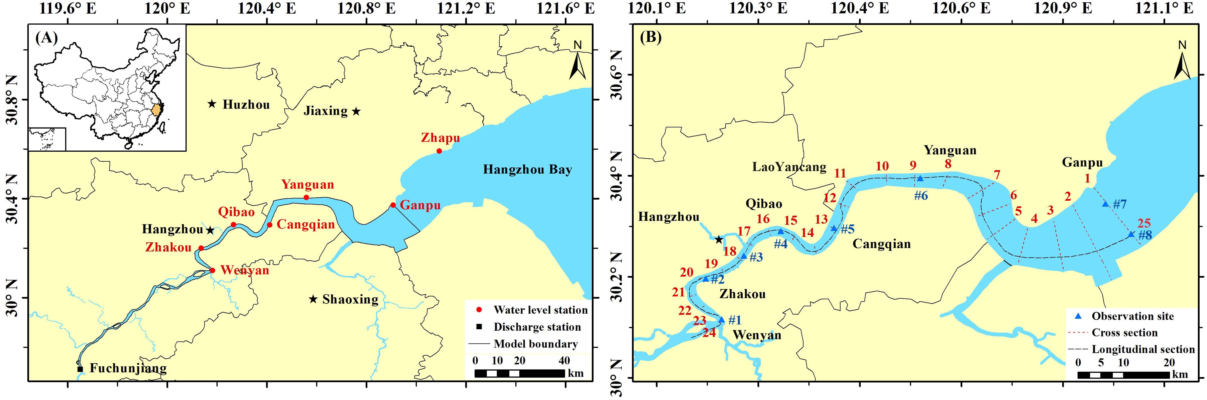
Figure 1. A map of the Qiantang Estuary. (A) Location of the long-term monitoring stations; (B) Locations of ship-born observation sites and analysis sections. The solid black line represents the scope of the study area, the red squares represent long-term water level monitoring stations, the black square represents long-term runoff discharge monitoring station, the blue triangles represent short-term ship-born observation stations (May 2012) for velocity, salinity and SSC, and the red and black dashed lines represent the cross and longitudinal sections used for results analysis.

2 Materials and methods

2.1 Study area

The Qiantang Estuary (119.6°-121.8°E and 29.7°-30.9°N) is the largest estuary along the East China Sea, with a total length of 282 km from Fuchunjiang hydropower station to the mouth of the Hangzhou Bay (Figure 1A). Based on its hydrodynamic characteristics, the estuary can be divided into three reaches (Li et al., 2020): runoff-dominated reach (from Fuchunjiang hydropower station to Wenyan, 78 km), tidal current and runoff affected reach (Wenyan to Ganpu, 120 km), and tide-dominated reach (Ganpu to estuary mouth, 84 km). This paper focuses on the reach influenced by both tidal currents and runoff, from Wenyan to Ganpu. A total of 25 analysis sections are set up for result analyses, and the locations of section are shown in Figure 1B.

The Qiantang Estuary is a typical funnel-shaped estuary, with its width narrowing from 100km at the estuary mouth to about 20 km at Ganpu, which makes it a worldwide famous macro-tidal estuary. The multi-year average tide range at Ganpu is 5.62m, and the maximum tide range can reach up to 9m. Meanwhile, the multi-year average level of runoff discharge (Q) is approximately 952 m³/s, indicating that the influence of runoff is significantly weaker than that of tidal currents, resulting in more severe saltwater intrusion in the Qiantang Estuary than in other tidal estuaries. Saltwater intrusion in the Qiantang Estuary is more extensive than in most estuaries, with saltwater extending as far as 200 km upstream from the mouth of Hangzhou Bay during spring tides (Li et al., 2019). The saltwater intrusion of the Qiantang Estuary exhibits significant seasonal variation, with high flow and low salinity during the wet season (April to July) and low flow and high salinity during the dry season (August to February) (Han et al., 2012; Pan et al., 2014).

The bedload of the Qiantang Estuary primarily consists of well-sorted fine sand (mean diameter ranging from 0.02 to 0.04 mm near Luchaogang) and clay (mean diameter ranging from 0.004 to 0.016 mm at Ganpu), which is prone to erosion and deposit under strong tidal currents (Guo et al., 2012). The mean SSC in runoff-dominated reach (upstream of Wenyan) is only 0.2-0.4 kg/m³ with the total annual average sediment transport amount of 6.68 × 10⁶ tons. However, in the tide-dominated section near Ganpu, the average SSC can reach 3-4 kg/m³, and the total quantity of sediment transport is as high as 1 × 10⁷ tons per tidal cycle (Chen et al., 1990). Therefore, the suspended sediment in the Qiantang Estuary mainly originates from Hangzhou Bay and is primarily controlled by tidal current dynamics. A great amount of deposited sediment formed a large sandbar in the upper and middle reach of the Qiantang Estuary, with a length of approximately 130 km longitudinally and a height of 10 m above the estuary bed at the top part near Cangqian (Xie et al., 2018).

2.2 Field data

Three datasets of different periods were collected for this study. Dataset 1 comprises the daily discharge series of the Fuchunjiang hydropower station from 2011 to 2012, used to determine the upstream boundary conditions. Dataset 2 is the field observed data from May 23 to May 31, 2012, used for model building and validation. Dataset 2 includes hourly tidal level data from 6 hydrological stations (Ganpu, Yanguan, Cangqian, Qibao, Zhakou, and Wenyan) and hourly velocity, salinity, and SSC sampled at three layers (surface, medium and bottom) from 8 ship-born observation sites (#1- #8) during spring, medium, and neap tide, each covering two complete tidal cycles. Dataset 3 consists of daily tidal level and salinity data at the Ganpu station from August 25 to September 10, 2011, including a complete semimonthly tidal cycle, used for experimental boundary conditions. The locations of monitoring stations and observation sites are shown in Figure 1.

Based on observational data from May 2012, Table 1 summarizes the maximum depth-averaged salinity and SSC at each observation site during spring, medium, and neap tides. During the observation period, Q is 1330-2320 m³/s, averaging 1736 m³/s. As shown in Table 1, the salinity and SSC in the Qiantang Estuary generally decrease from downstream to upstream. Notably, the maximum SSC values exceed salinity in the reach upstream of Yanguan (#6), particularly between Qibao and Cangqian (#4-#5).

Table 1

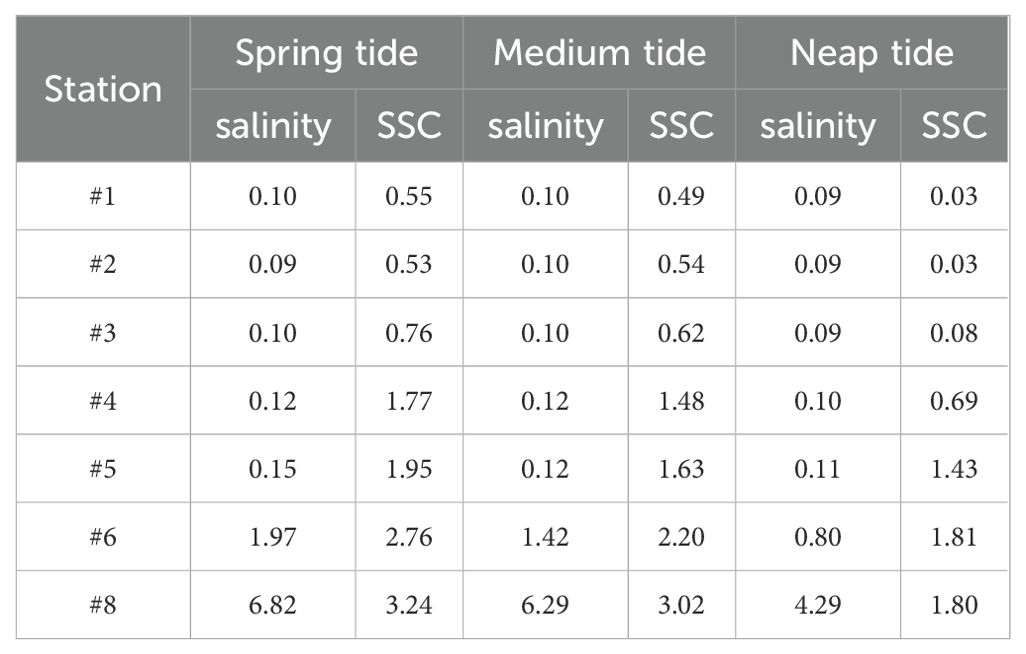
Table 1. Longitudinal variation of maximum salinity and SSC (ppt and kg/m³).

For instance, at Cangqian (#5), the flood duration is shorter than the ebb duration due to the tidal wave deformation, while the flood velocity exceeds the ebb velocity. During spring tide, the average flood velocity is 0.88 m/s, approximately 1.7 times the average ebb velocity of 0.52 m/s. The SSC and velocity curves exhibit similar patterns, with the SSC peaks occurring 1 hour after the peak flood. The salinity peaks lag the sediment peaks by about 2 hours, appearing around 1 hour after flood slack. The maximum SSC can reach 1.95 kg/m³ at Cangqian, significantly higher than the maximum salinity of 0.15 ppt. During spring tide, the tidal average salinity from Qibao to Yanguan ranges from 0.91 to 0.64 ppt, while the tidal average SSC ranges from 0.69 to 1.24 kg/m³. The contribution of SSC to water density significantly exceeds that of salinity in the Qibao to Cangqian reach, which can be more than 6 times that of salinity. Therefore, the impact of sediment on water density cannot be ignored in the salinity simulation of the Qiantang Estuary.

2.3 3D numerical model

2.3.1 Governing equations

The Qiantang Estuary is characterized by strong tidal currents and high sediment concentration, where the influence of SSC on water density cannot be ignored. Sediment transport is a 3D phenomenon. The settling velocity and the near-bottom interaction could generate vertical gradients of SSC (Cancino and Neves, 1999), consequently leading to changes in the distribution of baroclinic gradients in water column. Currently, most 3D numerical models of estuarine salinity have adopted the baroclinic mode (Brice et al., 2005; Rodrigues and Fortunato, 2017; Zhou et al., 2020; Jeong et al., 2022), but there are still many estuarine sediment models using the barotropic mode (Yu et al., 2014; Wang and Pan, 2018; Chen et al., 2020), neglecting the pressure changes caused by the uneven spatial distribution of SSC. Considering the significant variations in both salinity and SSC from Hangzhou Bay to Zhakou, it is necessary to account for the baroclinic effects induced by these two factors. Therefore, we simultaneously consider the influence of SSC and salinity on fluid density, and the density ρ is defined as Equation 1:

$\begin{array}{ll}\rho ={\rho }_0+({\rho }_s/{\rho }_0-1)S+({\rho }_c/{\rho }_0-1)C& (1)\end{array}$

where ${\rho }_0$, ${\rho }_s$ and ${\rho }_c$ are the specific density of water, salt and sediment, and S and C are the concentration of salt and suspended sediment. Based on this, a 3D model coupling current, SSC and salinity is established, with governing equations as shown in Equations 2-4. Equations 2-4 represent the continuity equation, momentum equation and material transport equation respectively.

$\begin{array}{ll}\frac{\partial \rho }{\partial t}+\text{∇}·(\rho \mathit{\text{V}})=0& (2)\end{array}$

$\begin{array}{ll}\frac{\partial \rho V}{\partial t}+\text{∇}·(\rho \mathit{\text{V}}\mathit{\text{V}})=\rho f+\text{∇}(\rho gZ)+\text{∇}·({\mu }_t\text{∇}\mathit{\text{V}})& (3)\end{array}$

$\begin{array}{ll}\frac{\partial \phi }{\partial t}+\text{∇}·(\phi \mathit{\text{V}})=\text{∇}·(ϵ\text{∇}\phi )+{\phi }_s& (4)\end{array}$

where $\phi =(S,C)$ represents the concentration of transported material, ${\phi }_s$ is the source-sink term for the transported material, ϵ is the diffusion coefficients, t is time, $\text{∇}$ is the Hamiltonian operator, V is the velocity vector, and ${\mu }_t$ is the turbulent viscosity in horizontal or vertical direction.

When substitute Equation 1 into Equations 2-4., the continuity and momentum equations are coupled with material transport equation for the fluid density ρ is related to the salinity and SSC. In the momentum equation (Equation 2), the pressure gradient term $\text{∇}(\rho gZ)$ varies not only with the depth Z but also with the density ρ, which represent the effect of baroclinic pressure. In summary, the numerical model presented in this paper reflects the strong coupling of tidal flow dynamics, salinity and suspended sediment, and the baroclinic effect induced by variations in salinity and SSC.

2.3.2 Model setups

The computational domain of the model extends from the Fuchunjiang hydropower station to the Ganpu section, covering the whole tidal current and runoff affected reach, with a total length of 197 km and an area of 779 km². In the horizontal direction, we used an orthogonal curvilinear grid with a total count of approximately 387 million, as shown in Figure 2A. The grid resolution gradually increases from a maximum of 700m at the downstream boundary to less than 150m upstream, and the minimum length of grids in the focus study area (from Qibao to Yanguan) is about 50m. In the vertical direction, the model adopts a boundary-fitted σ-coordinate system and is divided into 12 layers. The thickness of each layer from surface to bottom accounts for 10%, 10%, 10%, 10%, 10%, 10%, 10%, 10%, 10%, 5%, 3%, and 2% of the total water depth, respectively. The computational time range of the model spans from May 15, 2012, 00:00, to June 1, 2012, 00:00, with a time step of 15 seconds. And the model stabilization period is determined to be 15 days based on previous stability experiments, ensuring adequate stabilization.

Figure 2

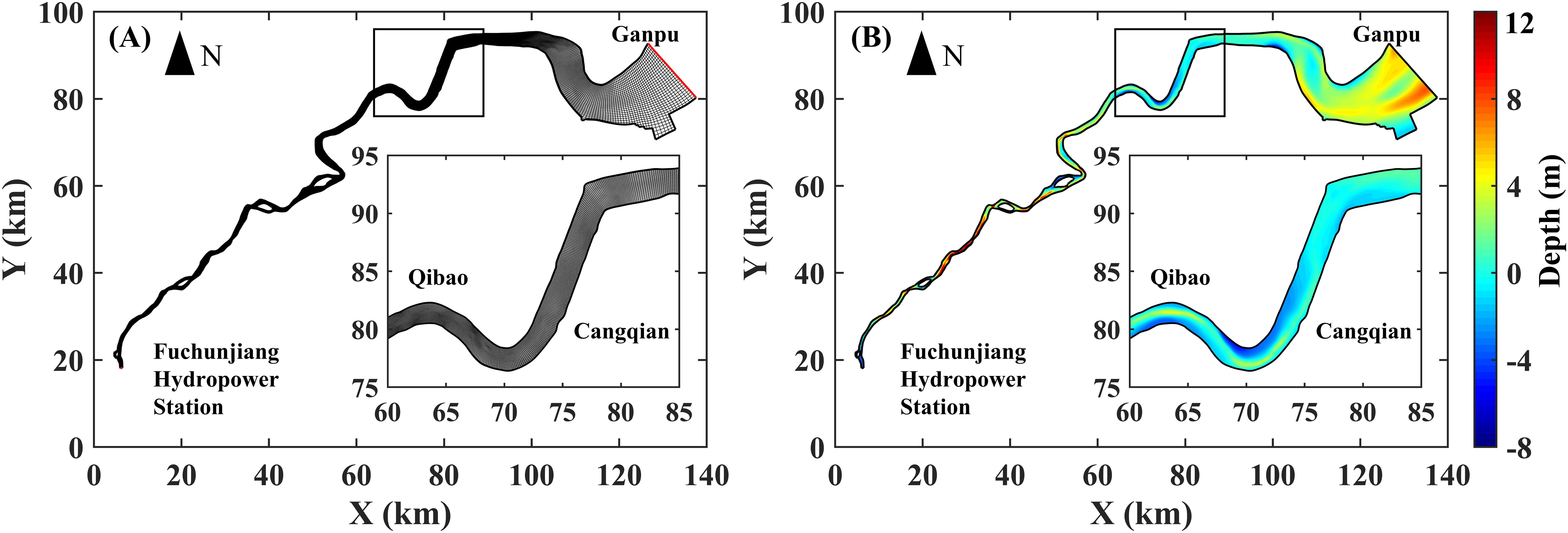
Figure 2. Model grids and bathymetry. (A) domain and horizontal grids; (B) bathymetry.

The bathymetry adopted in the model is based on the 1:10,000 topographic data (Figure 2B), and the threshold depth for dry-wet classification is set to 0.2 m considering the complex topographic variation in Qiantang Estuary. The model has two open boundaries, as indicated by the red solid line in Figure 2A. The upstream open boundary at Fuchunjiang hydropower station is discharge-controlled and the boundary condition is determined by the daily average discharge series from Dataset 1. Since the discharged water is primarily fresh water used for power generation with very low sediment content, we set the salinity at upstream boundary to 0 ppt. The downstream open boundary at Ganpu section is water level-controlled, employs measured water levels and salinity series from the Ganpu (Dataset 2 and 3). The conditions of SSC at two open boundaries are calculated by the logarithmic sediment transport capacity formula (Equation 5) based on the current velocity and water depth obtained from hydrodynamic numerical simulations (Sun et al., 2018).

$\begin{array}{ll}{C}_{*}=m\ln (u^b/gh{\omega }_s)& (5)\end{array}$

In Equation 5, m and b are empirical parameters calibrated through measured data, with values of 1.9 and 5.75. The sediment settling velocity ${\omega }_s$ is calculated using Equation 6,

$\begin{array}{ll}{\omega }_s=\{\begin{array}{ll}\frac{{\omega }_{s,max}}{2}\left(1-\cos \left(\frac{\pi S}{S_{max}}\right)\right)+\frac{{\omega }_{s,o}}{2}\left(1-\cos \left(\frac{\pi S}{S_{max}}\right)\right)\hfill & \text{when\hspace{0.17em}}S\le S_{max}\hfill \\ {\omega }_{s,max}\hfill & \text{when\hspace{0.17em}}S>S_{max}\hfill \end{array}& (6)\end{array}$

where ${\omega }_{s,o}$ is the settling velocity in fresh water, and ${\omega }_{s,max}$ is the maximum flocculation settling velocity in saltwater, with reference values obtained from sediment settling experiments at the mouth of the Yangtze River Estuary (Wan et al., 2015), taken as 0.05 and 0.75 mm/s, respectively. $S_{max}$ represents the salinity at which flocculation settling velocity reaches ${\omega }_{s,max}$, with values set to 15 ppt based on the research findings in the Qiantang Estuary (Wu et al., 2007). Manning coefficient is used for the bottom friction calculation, and its value is set as 0.010-0.015 according to previous research (Guo et al., 2012; Wang and Fellow, 2018) and then and calibrated in validation. The model adopts a k−ϵ turbulent closure model, and employs the Partheniades-Krone equation (Partheniades, 1965) to calculate the erosion and deposition for sediment. The model’s bedload utilizes uniform cohesive sediment and the median diameter is set as 0.02 mm based on previous studies (Huang et al., 2022).

The model adopts a cold start, with an initial water level of 4 m and an initial SSC of 0 kg/m³. The initial salinity increases from 0 ppt at the upstream boundary to 15 ppt at the downstream boundary. To ensure the model achieves complete stability before the validation period, we set up a tide circle of 15 days based on observed data. It guarantees a smooth transition between the model’s stabilization period and the validation period or research period. To eliminate the interference of topographic changes on salinity simulation, the model doesn’t perform morphology correction, aiming to separately analyze the influence of sediment-induced density change on salinity simulation.

2.3.3 Validation

Dataset 2 is used for model validation, during which the Q from the Fuchunjiang hydropower station ranged from 1330 to 2640 m³/s, and the tidal range at the downstream Ganpu boundary varied between 5.19 and 7.51 m. The salinity ranges during spring, medium, and neap tides were 1.70-6.82, 1.86-6.28, and 1.65-4.29 ppt, respectively. The validation results for Cangqian and Yanguan stations (#5 and #6) during spring tides are shown in Figure 3. Among them, 89% of the points had error less than 10cm in tidal level, 83% had a relative error below 10% in velocity, 85% had a relative error of less than 30% in SSC, and 93% in salinity.

Figure 3

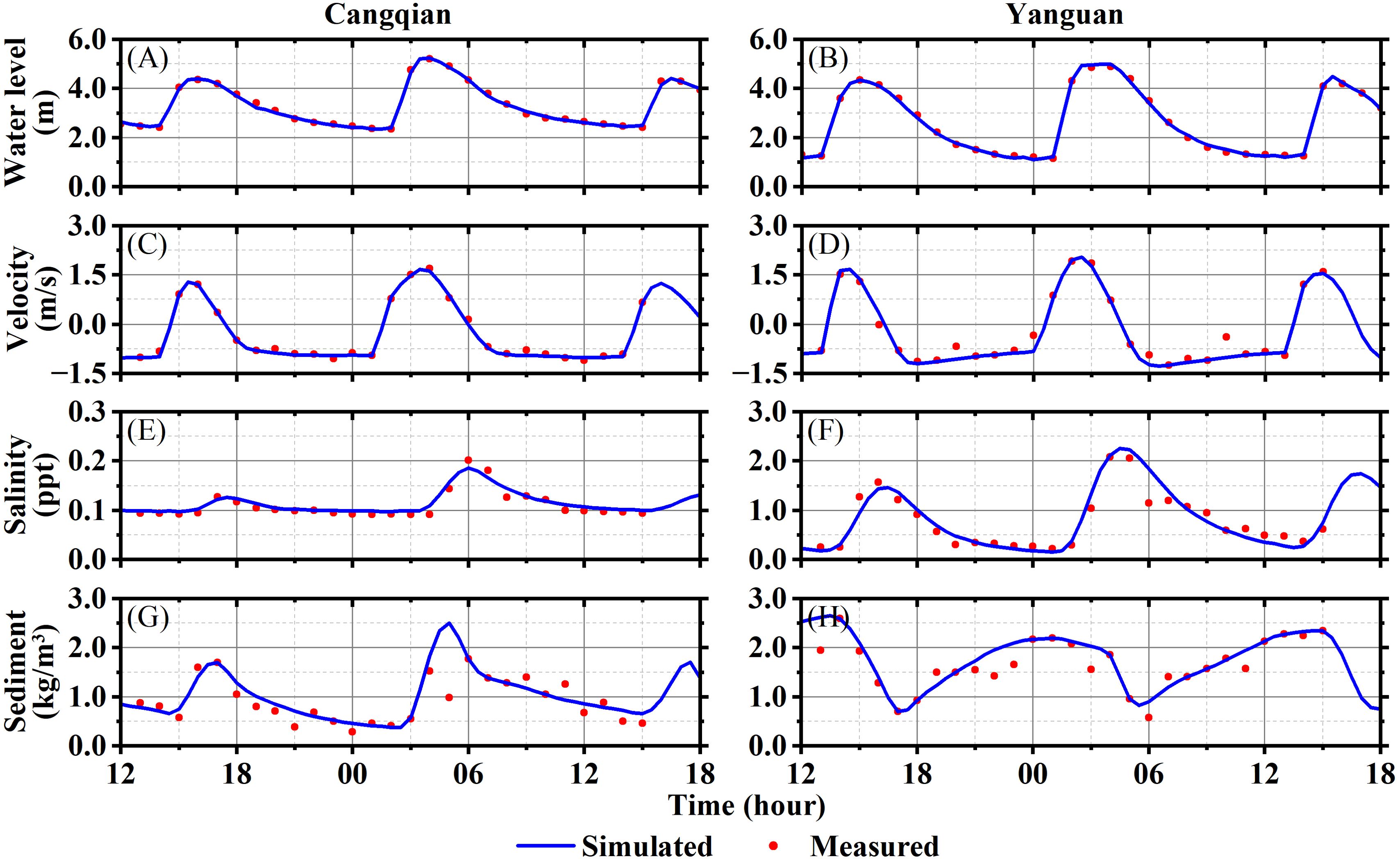
Figure 3. Comparison of the simulated and measured results at Cangqian and Yanguan stations during spring tide. (A, B) Water level; (C, D) Velocity; (E, F) Salinity; (G, H) SSC.

Two evaluation indicators, correlation coefficient (CC) and root mean square error (RMSE), are employed to evaluate the performance of the model. The calculated results for each indicator are presented in Figure 4. For the water level of each station, the CC value is all above 0.9, and the RMSE value is less than 0.2, indicating good simulation results. For velocity, except for the bottom layer at #3 which exhibited a lower CC value, all other sites have CC values above 0.75, and the flow directions in all sites are well-fitted. Most of the salinity simulation results show CC values above 0.8. Regarding simulation results of SSC, except for the bottom layer at point #1, the CC values at other points are all above 0.7, with higher RMSE values at the bottom layer compared to the surface. The simulation results of the model show a qualitatively good agreement with the observed data.

Figure 4

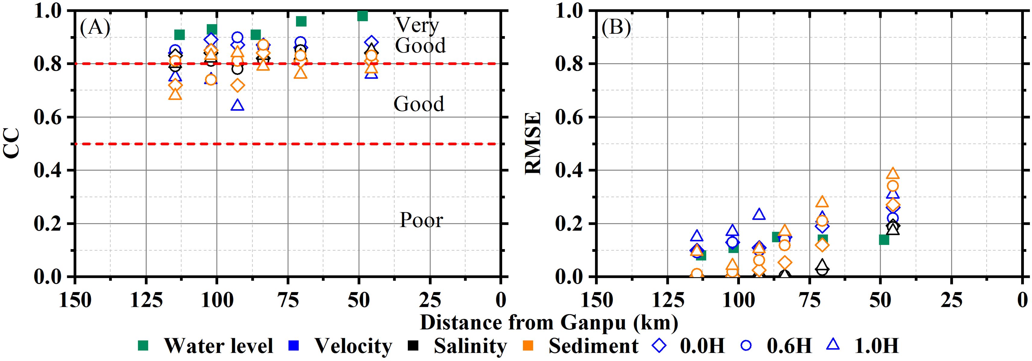
Figure 4. The distribution of evaluation indicators. (A) CC (B) RMSE. For CC, values greater than 0.8 indicate a strong correlation, while values below 0.5 indicate a weak correlation. And for RMSE, smaller values are more desirable.

2.4 Settings of numerical experiments

In this paper, two groups of numerical experiments are designed to study the density effect of SSC on salinity simulation. For case 1, both the effect of SSC and salinity on fluid density are considered, while only the density effect of salinity is considered in case 2. The salinity simulation results of case 1 and 2 are expressed as S_C and S₀, respectively. The other subscript _₀ and __C in the following text also mean the same. The details for each experiment are shown in Table 2.

Table 2

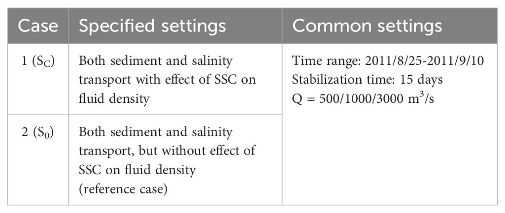
Table 2. List of configurations of the numerical experiments.

The analysis period is from September 1 to September 9,2011, including three tidal types of large, medium, and neap tide. The downstream boundary conditions are determined by dataset 3, while the Q is selected as 500 m³/s, 1000 m³/s and 3000 m³/s for dry season, multi-year annual average level and wet season based on statistics result from dataset 1.

3 Results

3.1 Effect of SSC on salinity under different tidal conditions

3.1.1 Variations of salinity and SSC with different tide ranges

The simulation results of three sections (No. 10, 12 and 14) located near Laoyancang, Cangqian and Qibao are selected to analyze the variation characteristics of each element in the tidal cycle under different tidal conditions. The time-varying curves of the water level and cross-sectional average velocity, SSC, and salinity (S_C) at these sections under dry season runoff (Q = 500 m³/s) are shown in Figure 5.

Figure 5

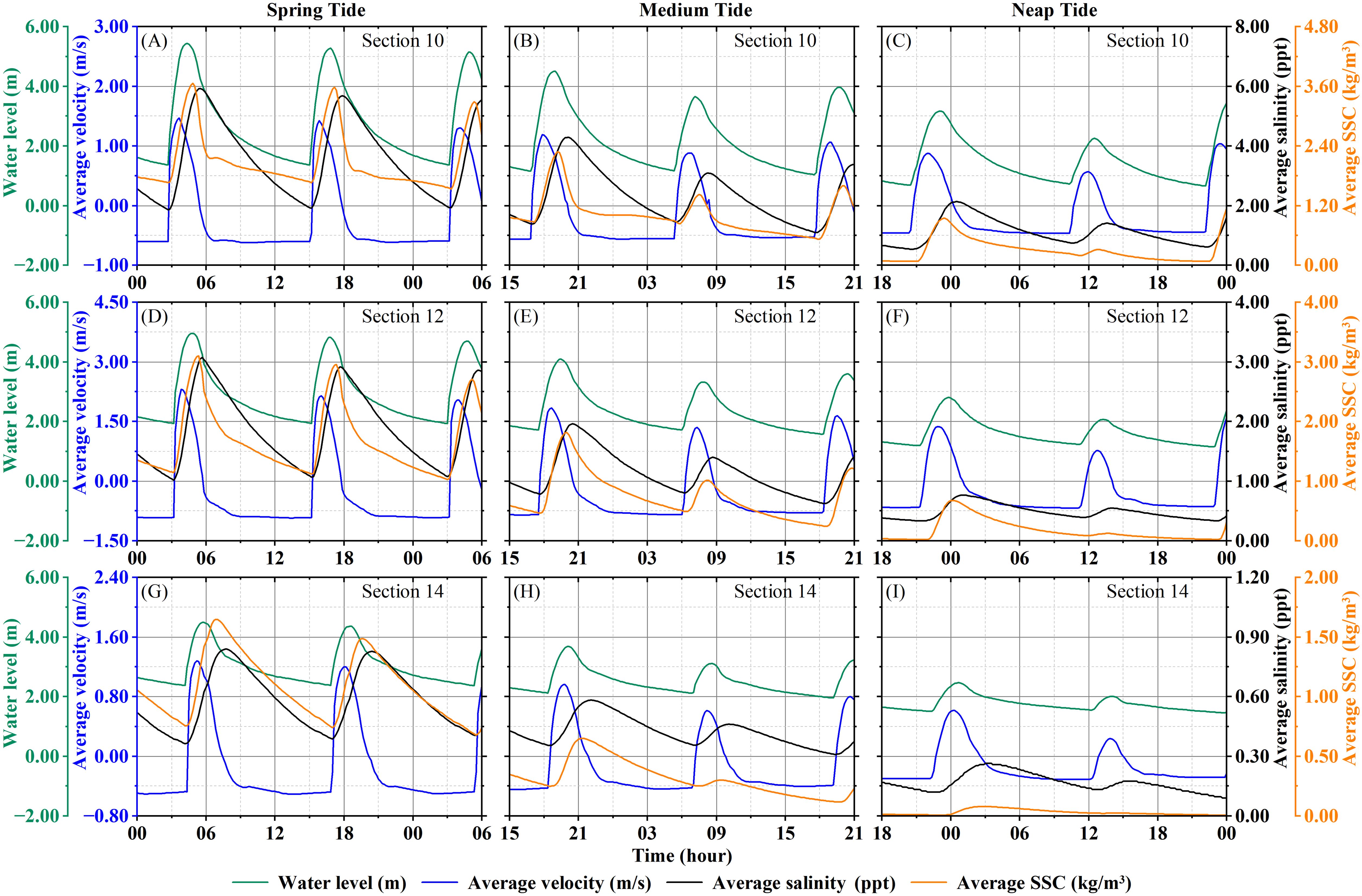
Figure 5. The temporal variations of water level, velocity, S_C, and SSC in Sections 10-14 under different tidal conditions (Q = 500 m³/s). (A-C) Section 10; (D-F) Section 12; (H-I) Section 14.

According to Figure 5, there is an obvious tidal wave deformation between Sections 10 and 14. The flood duration is significantly shorter than the ebb duration, with a ratio ranging from 0.16 to 0.24. Flood slack generally follows high tide by 50-70 minutes, while ebb slack occurs only 0-20 minutes after low tide. The peak flood occurs within 2 hours after low tide, while peak ebb isn’t significant during ebb tide. The curves of S_C and SSC exhibit a single peak pattern, with the peak of S_C generally appearing at the flood slack, while the peak of SSC appears 1.5-2 hours after the peak flood. The variations of S_C and SSC are primarily controlled by the strength of tidal dynamics. During spring tide, the peak S_C is 2.6-4.2 times of that during neap tide, while the peak SSC can reach 3-16 times higher than that during neap tide.

Considering the peak of SSC occurs approximately 2 hours after peak flood in Section 12 (Cangqian), close to the flood slack, and the peak of S_C is also close to this moment, we selected the simulation results when Section 12 at flood slack during spring, medium and neap tide to analyze the longitudinal distribution of S_C and SSC, as shown in Figure 6. Figures 6A–C reveals a gradual decrease in S_C from downstream to upstream, with the contour lines of S_C nearly vertical, indicating a strong mixing effect in the Qiantang Estuary, resulting in an almost vertically uniform distribution of S_C. As the tidal range diminishes, the S_C along the longitudinal section reduces generally, with the position of the 3.0 ppt contour moving about 12 km downstream. There are two high SSC zones within 50-70 km and 20-40 km from Ganpu, with the maximum SSC in the bottom layer reaching 8.21 kg/m³ (Figures 6D–F). In these regions, the impact of SSC on fluid density variation is greater than that of salinity, especially at the bottom during spring tide. Since the sediment transport in the Qiantang Estuary is mainly controlled by tidal dynamics, the SSC significantly decreases as the tidal range reduces, with the high SSC zones also moving downstream. The SSC during neap tide generally is below 1.5 kg/m³.

Figure 6

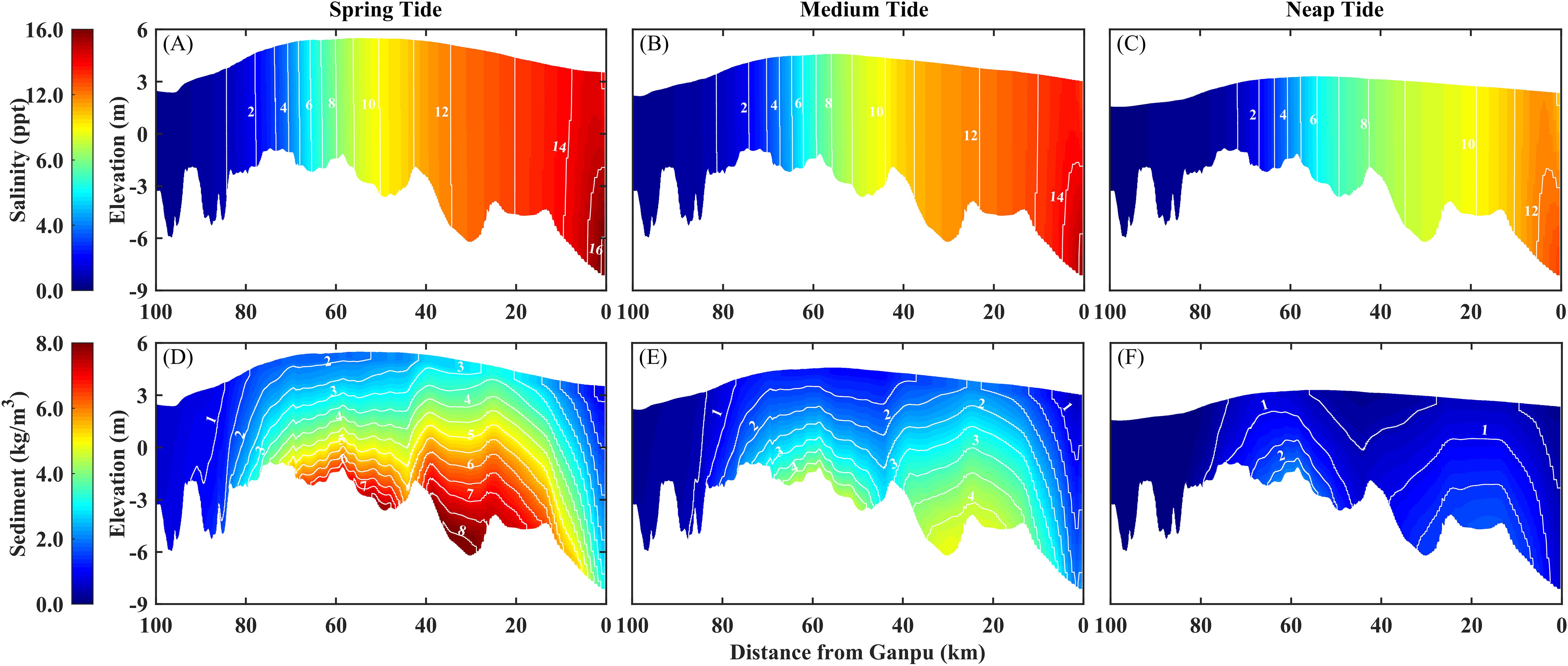
Figure 6. Longitudinal distribution of S_C and SSC at flood slack of Section 12 (Cangqian) under different tidal conditions (Q = 500 m³/s). (A-C) SC; (D-F) SSC.

3.1.2 Change of maximum salinity with SSC and tide ranges

To analyze the impact of SSC on salinity simulation, we compared the depth-averaged simulation results of S_C and S₀, and calculated the value of salinity difference ΔS (ΔS = S₀ > S_C). The distributions of the maximum ΔS during spring, medium, and neap tides under dry season runoff (Q = 500 m³/s) are shown in Figure 7.

Figure 7

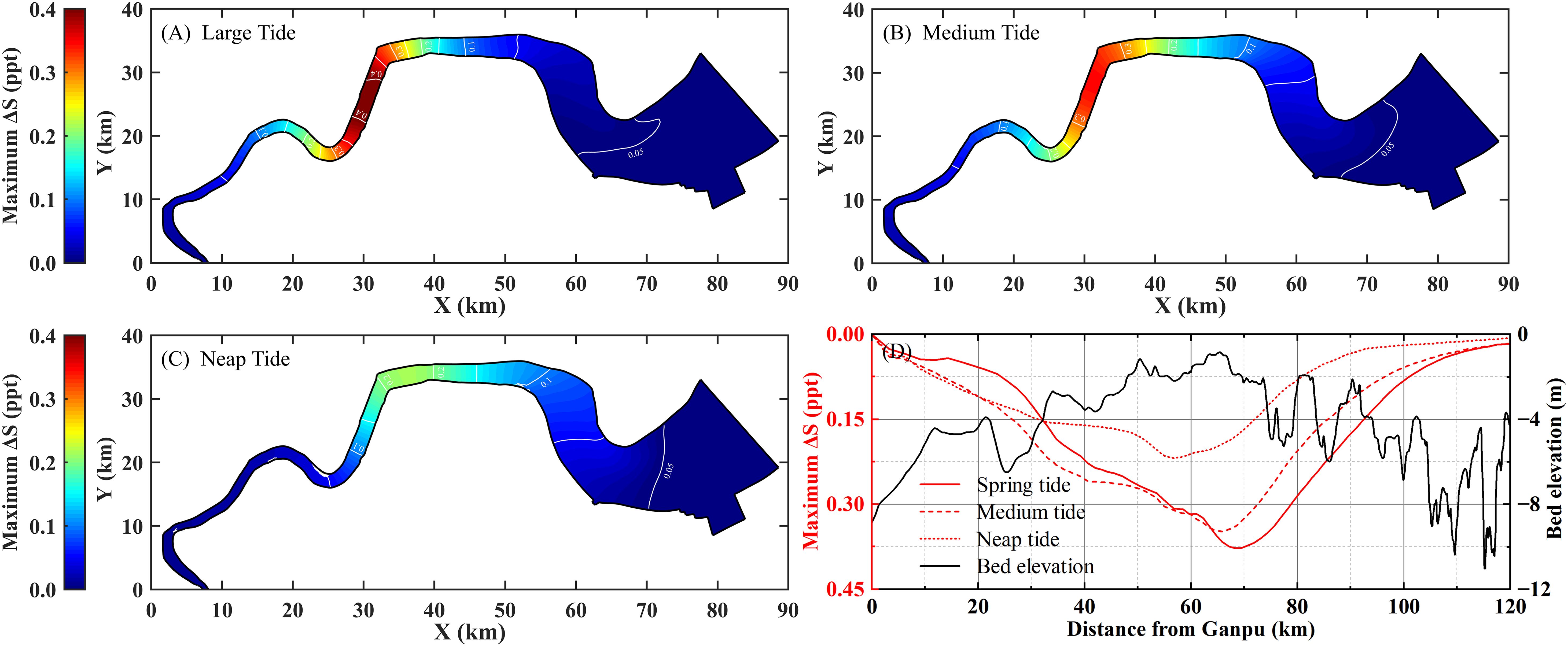
Figure 7. Horizontal and longitudinal distribution of the maximum ΔS caused by SSC under different tidal conditions (Q = 500 m³/s). (A-C) Horizontal distribution; (D) Longitudinal distribution.

As indicated in Figure 7, the ΔS values within the study area are all positive, namely S₀ > S_C, indicating that the fluid density increase caused by SSC leads to a decrease in the simulated salinity results. In other words, suspended sediment can weaken the saltwater intrusion in the estuary. Taking Section 12 as an example, the maximum values of salinity reduction during spring, medium and neap tides are 0.40, 0.34, and 0.12 ppt, with reduction rates of 8.9%, 12.8%, and 12.3%, respectively. Therefore, the impact of SSC on salinity variation is considerable and cannot be ignored.

In Figure 7D, the ΔS caused by SSC initially increases and then decreases from downstream to upstream in general. The peak of ΔS is mainly located between Cangqian and Yanguan and is relatively consistent with the locations of the top of the underwater sandbar. During spring, medium and neap tides, the maximum ΔS values are 0.42, 0.35, and 0.22 ppt, occurring at 78, 73, and 64 km upstream of Ganpu. And the length of reach where ΔS exceeds 0.15 ppt can reach 65, 63, and 44 km, respectively. Comparing the ΔS distributions under different tidal conditions reveals that as the tidal range at the downstream boundary decreases, the ΔS peak value decreases and moves downstream, and the length of the reach with significant ΔS is also shortened. The main reason is that the SSC decreases as tidal dynamics weaken, and its influence on saltwater intrusion weakens accordingly.

3.2 Effect of SSC on salinity under different runoff conditions

3.2.1 Variations of salinity and SSC with different runoffs

The time-varying curves of the water level and cross-sectional average velocity, SSC, and S_C at these sections during spring tide under different runoff conditions (Q = 500, 1000 and 3000 m³/s) are shown in Figure 8. As the Q increases, the tidal range decreases and the high and low tide levels rise, which results in a significant reduction in the peak value of S_C. When the Q reaches 3000 m³/s, the S_C curves of Sections 12-14 approach 0 ppt and show no obvious fluctuations, indicating that these sections are outside the influence range of saltwater intrusion. Influenced by the increased Q, the SSC in Sections 10-14 exhibits a trend of first increase and then decrease. The SSC at the average flow condition (Q = 1000 m³/s) is approximately 1.3 times that under dry season runoff (Q = 500 m³/s). This pattern may be attributed to the combined effect of changes in tidal dynamics and sediment settling velocity influenced by salinity during flood tide. Meanwhile, the SSC during ebb tides increase relatively due to the increase in ebb tide flow velocity. Especially, Section 10 even shows a significant SSC peak during ebb tide when Q = 1000 m^3/s.

Figure 8

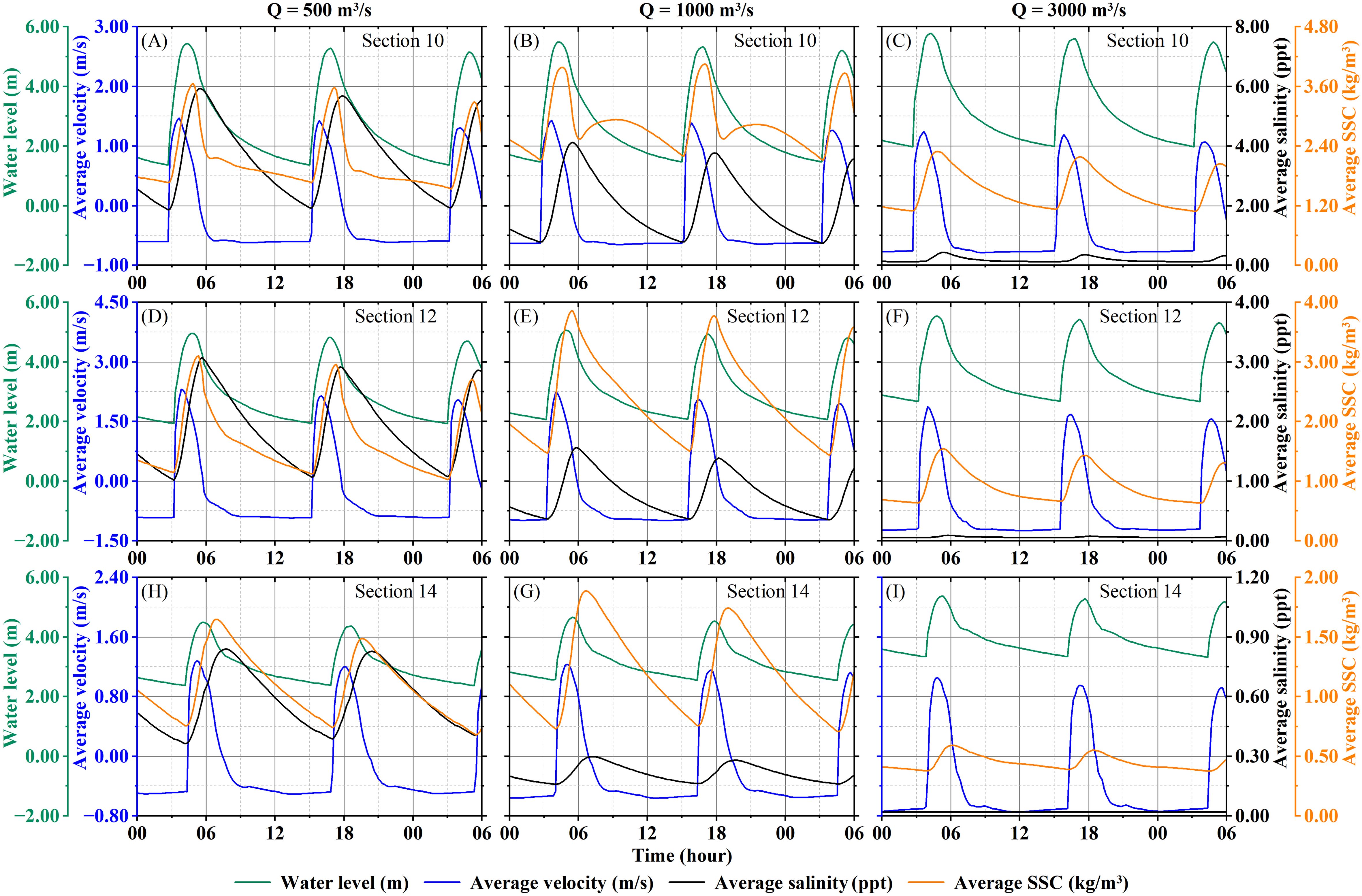
Figure 8. The temporal variations of water level, velocity, S_C, and SSC in Sections 10-14 under different runoff conditions (Spring tide). (A-C) Section 10; (D-F) Section 12; (H-I) Section 14.

The longitudinal distributions of S_C and SSC at the flood slack under different runoffs are shown in Figure 9. Influenced by increasing Q, the upstream water level rises significantly, and the S_C within 40 km from Ganpu is almost unchanged while the S_C in reach above 40 km from Ganpu decreases rapidly. It’s notable that there is a significant increase in SSC within the range of 65-80 km upstream from Ganpu when Q increases from 500m³/s to 1000m³/s, which is consistent with the analysis results for Sections 10-14 in Figure 8. However, as Q increases to 3000m³/s, the SSC along the longitudinal section decreases rapidly, and the high SSC zone moves downstream.

Figure 9

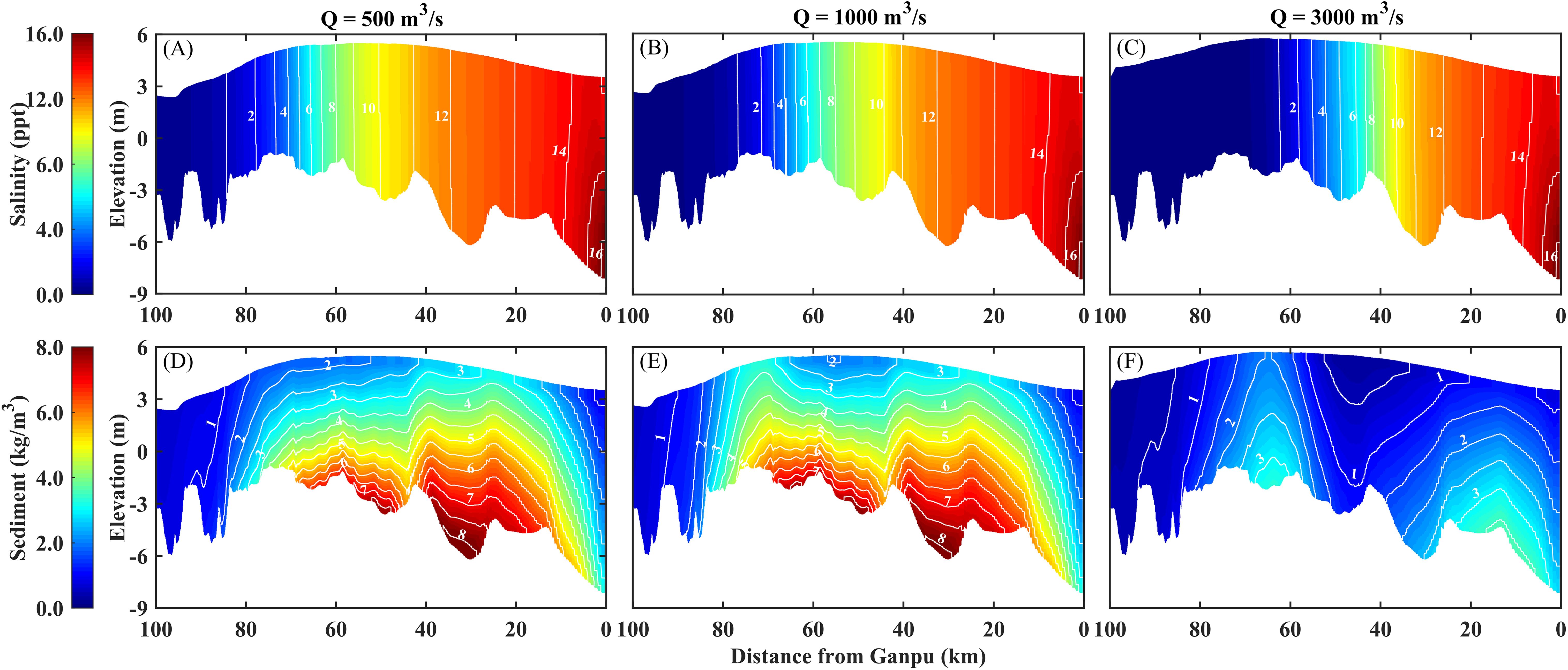
Figure 9. Longitudinal distribution of S_C and SSC at flood slack of Section 12 (Cangqian) under different runoff conditions (Spring tide). (A-C) SC; (D-F) SSC.

3.2.2 Change of maximum salinity with SSC and runoff

The distributions of the maximum ΔS during spring tide under different runoff conditions are shown in Figure 10. According to Figures 10A–C, with different runoffs, the simulated salinity results also decrease when considering the density effect of SSC, which is consistent with the analysis results obtained in Section 4.2. When Q is 500, 1000 and 3000 m³/s, the maximum values of ΔS induced by SSC is 0.40, 0.19 and 0.001 ppt, occurring at 78, 73, and 64 km upstream from Ganpu, close to the top of the underwater sandbar. And the length of reach where ΔS over 0.15 ppt can reach 65, 24, and 0.1 km, respectively. By comparing the ΔS distributions under different runoff conditions, it can be observed that as the Q decreases, the inhibition of SSC on saltwater intrusion weakened rapidly, with the ΔS peak decreasing and moving downstream, and the range of significant salinity reduction (ΔS > 0.15 ppt) narrowing apparently. When Q reaches 3000 m³/s, the maximum ΔS decreases to below 0.03 ppt, and the reduction rate is within 2%, indicating that the density effect of SSC on salinity is extremely weak and negligible.

Figure 10

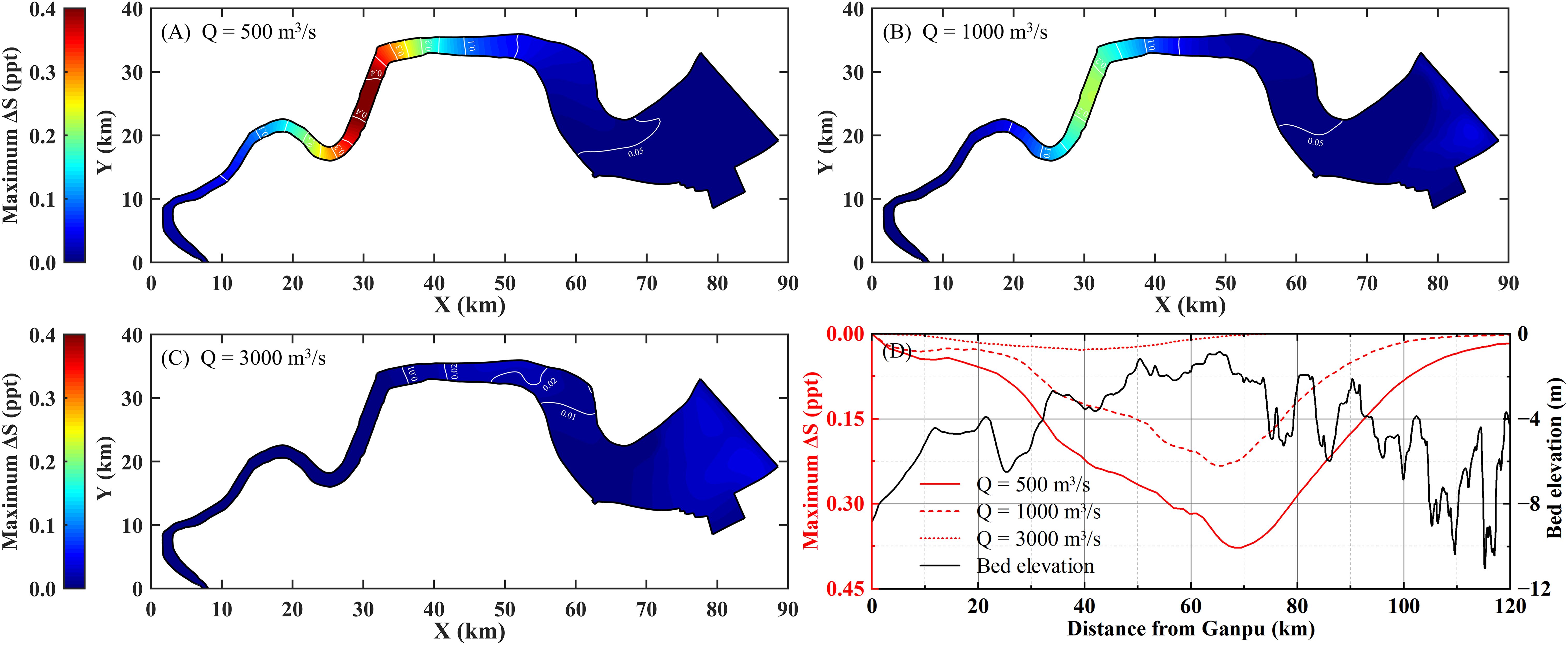
Figure 10. Horizontal and longitudinal distribution of the maximum ΔS caused by SSC under different runoff conditions (Spring tide). (A-C) Horizontal distribution; (D) Longitudinal distribution.

3.3 Longitudinal variation of maximum salinity contours

In principle, the chlorinity value of domestic water sources should be guaranteed to be below 0.25 g/L (equivalent to a salinity value of 0.45 ppt). We usually take the location where the maximum salinity can reach up to 0.45 ppt as the farthest point of saltwater intrusion, and the distance from this point to the downstream boundary is called the saltwater intrusion distance. Therefore, it’s of great significant to determine the maximum saltwater intrusion distance for protecting the water sources and designing water supply facilities.

Since the upstream salinity increases with the increase of tidal range or the decrease of Q, we selected the simulation results during spring tide under dry season runoff (Q = 500 m³/s) for statistics and obtained the distribution of the maximum S₀ and S_C in a tidal cycle, as shown in Figure 11. Simultaneously, we calculated the distances L from different salinity contour lines to the downstream boundary and analyzed the variation in the location of each contour, as shown in Table 3.

Figure 11

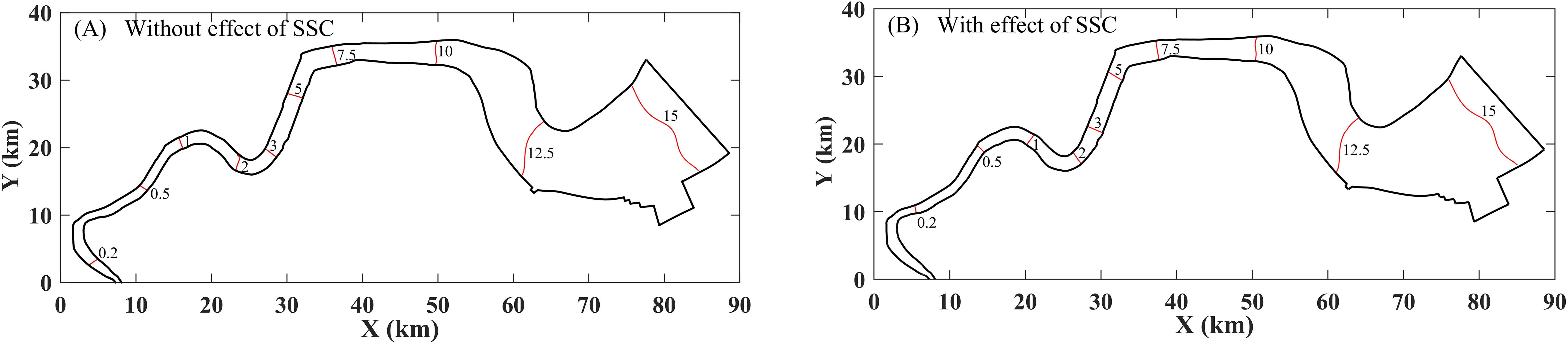
Figure 11. Variations of salinity contour locations caused by SSC. (A) Without effect of SSC; (B) with effect of SSC.

Table 3

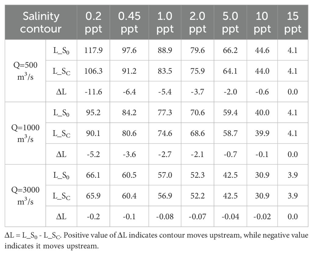
Table 3. Variation of salinity contour locations with the effect of SSC (km).

As indicated in Figure 11, the locations of each salinity contour move downstream due to the impact of SSC. According to Table 3, the contours below 1.0 ppt move downstream significantly, with the ΔL exceeding 5 km when Q is 500 m³/s. Influenced by SSC, the saltwater intrusion distance decreases from 97.6, 84.2 and 60.5 km to 91.2, 80.6 and 60.4 km when Q is 500, 1000, and 3000 m³/s, and the downstream moving distance is 6.4, 3.6 and 0.1 km, respectively. This indicates that when Q exceeds 3000 m³/s, the influence of SSC on saltwater intrusion distance can be almost negligible. However, during dry season, SSC has a significant impact on the simulation results of saltwater intrusion distance. And this situation corresponds to the most serious case of saltwater intrusion. Ignoring this effect in the numerical simulation would overestimate the prediction results of salinity, which can lead to misjudgments of the saltwater intrusion distance.

4 Discussion

4.1 Relation between the distribution of salinity difference and SSC

To explore the relationship between ΔS and SSC in the Qiantang Estuary, we analyzed the temporal and spatial correlation between these two factors. The time-series curves of ΔS induced by the SSC were calculated from simulated salinity results from Sections 10, 12 and 14 during spring tide under dry season runoff (Q = 500 m³/s) and then compared with the SSC curves to analyze their temporal correlation, as shown in Figure 12. The comparison reveals that the ΔS peak occurs between the peaks of S_C and SSC, and shifts closer to the peaks of S_C as moving upstream. Since the peaks of S_C and SSC are relatively close between Yanguan and Qibao, the time interval between the peaks of ΔS and SSC is generally within 10 minutes, indicating a high temporal correlation between the two distributions. Therefore, the change of ΔS is closely related to the value of SSC, especially during flood tide.

Figure 12

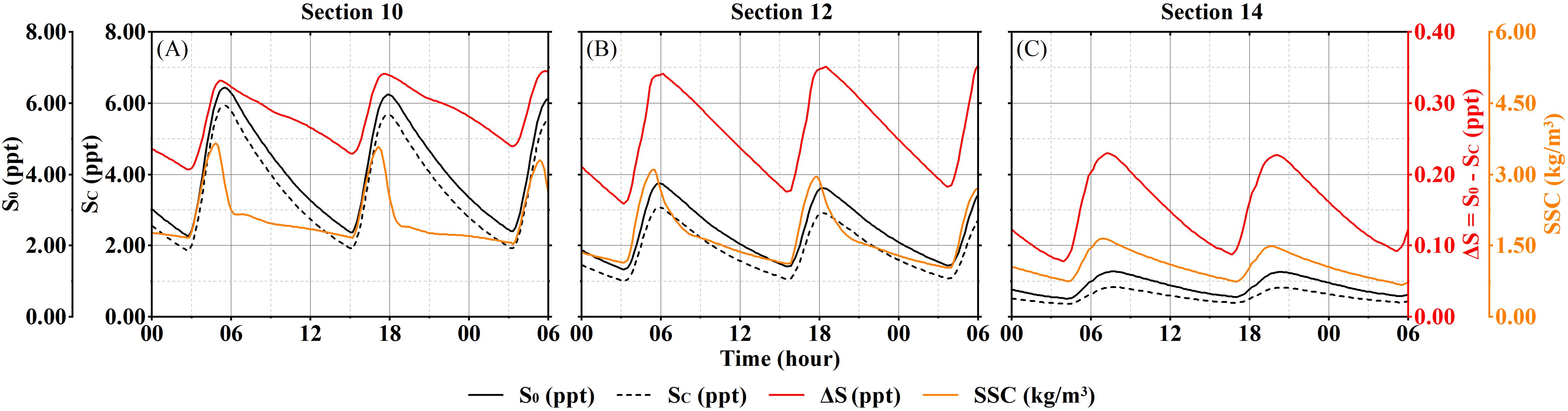
Figure 12. Temporal relationship between ΔS and SSC.

Considering that the peaks of ΔS and SSC curves do not occur simultaneously and the duration between the peaks varies among different sections, we took a complete tidal cycle (about 25 hours) as the period for time-averaging, which can eliminate temporal differences when analyzing the spatial relationship between ΔS and SSC. We calculated the tidal-averaged results of salinity ($\overline{S_0}$ and $\overline{{\text{S}}_{\text{C}}}$) and SSC ($\overline{\text{SSC}}$) at different sections from Ganpu to Wenyan, and then obtained the tidal-averaged salinity difference $\text{Δ}\overline{\text{S}}$ ($\text{Δ}\overline{\text{S}}=\overline{{\text{S}}_0}-\overline{{\text{S}}_{\text{C}}})$ of each section. The longitudinal distributions of $\text{Δ}\overline{\text{S}}$ and $\overline{\text{SSC}}$ under different tide and runoff conditions are shown in Figure 13.

Figure 13

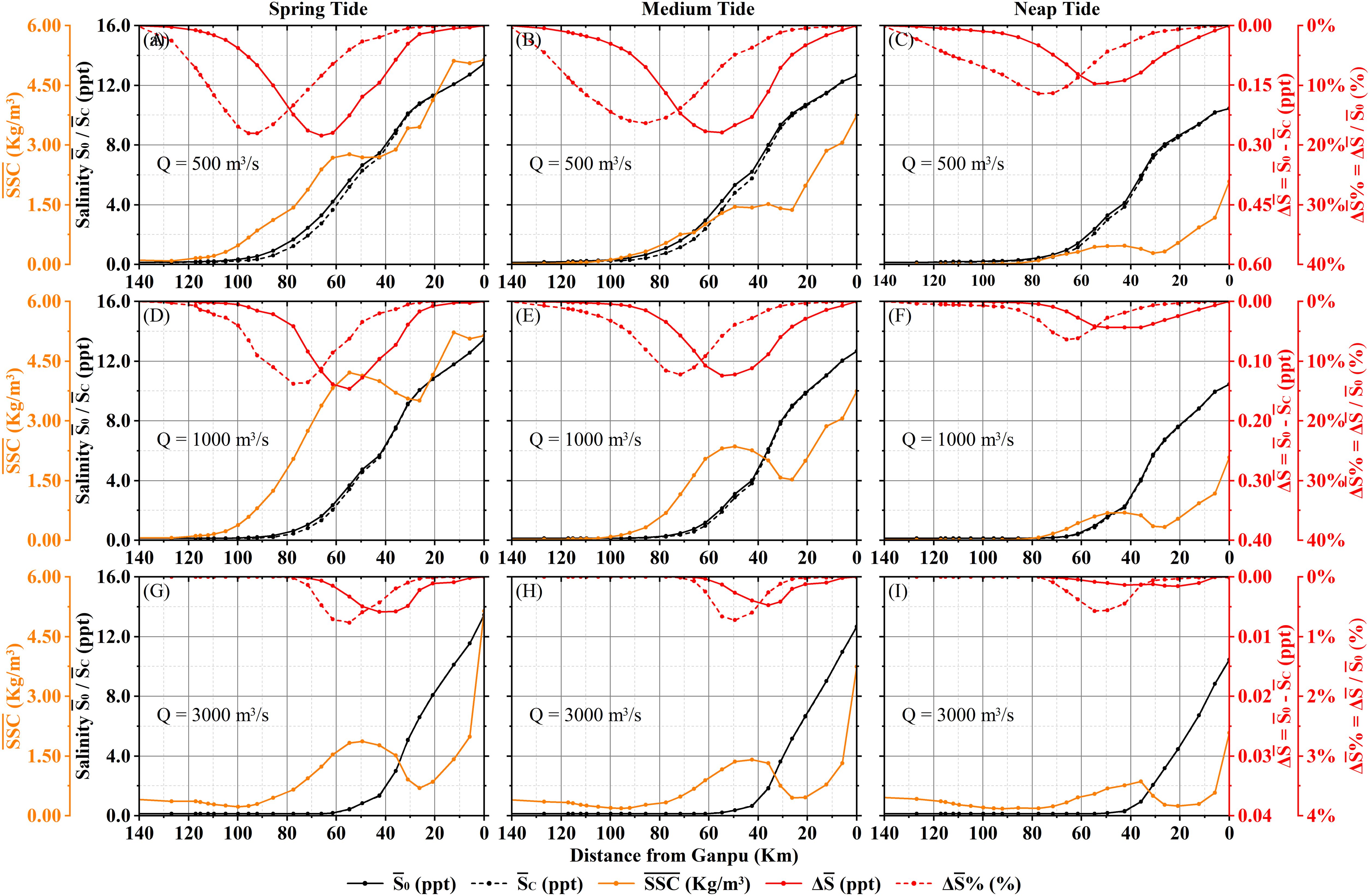
Figure 13. Spatial relationship between $\text{Δ}\overline{\text{S}}$ and $\overline{\text{SSC}}$. (A-C) Q = 500 m³/s; (D-F) Q = 1000 m³/s; (G-I) Q = 3000 m³/s; (A, D, G) Spring tide; (B, E, H) Medium tide; (C, F, I) Neap tide.

Generally, the $\text{Δ}\overline{\text{S}}$ included by SSC initially increases and then decreases from downstream to upstream in Figure 14, which is consistent with the longitudinal distribution of ΔS in Figures 7, 10. Its peak is located within 40-80 km from Ganpu, with a maximum value of 0.27 ppt occurring during spring tides when Q is 500 m³/s. Meanwhile, the position of $\text{Δ}\overline{\text{S\%}}$ ($\text{Δ}\overline{\text{S\%}}=\text{Δ}\overline{\text{S}}/\overline{{\text{S}}_0}$) peak lies at 30-40 km upstream of the $\text{Δ}\overline{\text{S}}$ peak. The maximum $\text{Δ}\overline{\text{S\%}}$ can reach up to 18%, corresponding to $\Delta \overline{\text{S}}$ of 0.08 ppt. The $\overline{\text{SSC}}$ generally decreases from downstream to upstream, but there is a distinct high concentration zone within 40-70 km from Ganpu. The maximum value of $\overline{\text{SSC}}$ reaches 4.19 kg/m³, occurring during spring tides when Q is 1000 m³/s.

Figure 14

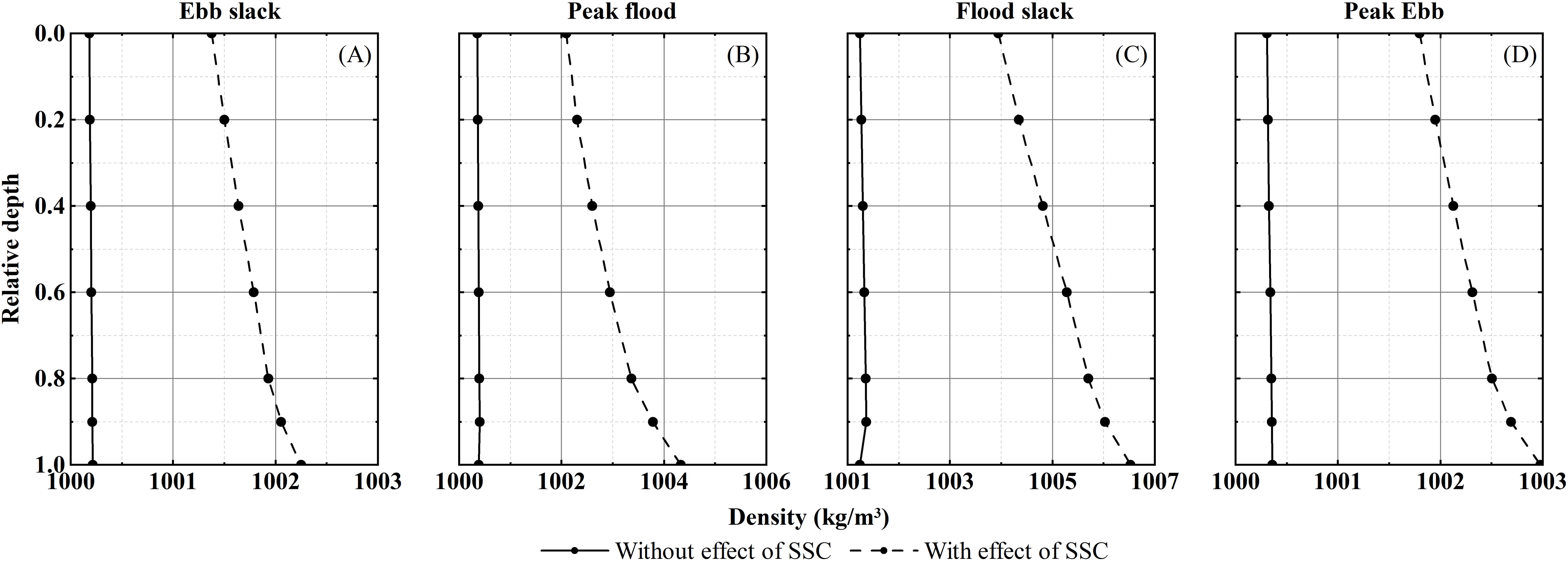
Figure 14. Variations in vertical density distribution induced by SSC at Section 12 during a tidal cycle (spring tide, Q = 1000 m³/s). (A) Ebb slack; (B) Peak flood; (C) Flood slack; (D) Peak ebb.

Overall, the peak locations of $\text{Δ}\overline{\text{S}}$ and $\overline{\text{SSC}}$ are relatively close, and essentially coincide under the annual average runoff (Q = 1000 m³/s), indicating a strong correlation between the longitudinal distributions of $\text{Δ}\overline{\text{S}}$ and $\overline{\text{SSC}}$. And the decrease in salinity is more significant in higher SSC zone. As the tidal range increases or the Q decreases, the high SSC zone moves upstream and the peak value of SSC increases, with its weakening effect on saltwater intrusion. It causes the $\text{Δ}\overline{\text{S}}$ peak to increase and move upstream accordingly, which is consistent with the results in Chapters 3.

4.2 Influence of SSC on density and turbulence diffusion

Previous studies have confirmed that high SSC can significantly change fluid density distribution and induce stratification, which suppresses the vertical turbulence intensity. To investigate the mechanism by which SSC influences salinity transport, we compared the simulation results of density distribution and vertical turbulent diffusion, analyzing their variations induced by SSC. Table 4 presents the tidal average density differences caused by SSC at Sections 10-14 during spring tides and shows SSC’s contribution to density under different runoff conditions. Additionally, we focused on section 12 (Cangqian), where the ΔS is most pronounced, to analyze the influence of SSC on density stratification and vertical eddy diffusion coefficient, as shown in Figures 14, 15. The density stratification coefficient N is calculated by Equation 7.

Table 4

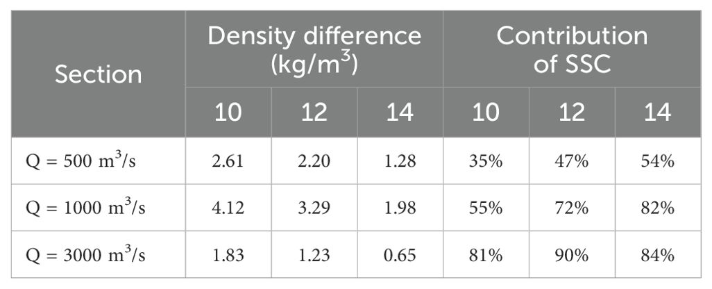
Table 4. Changes of tidal-averaged density induced by SSC (Spring tide, Q=1000 m³/s).

Figure 15

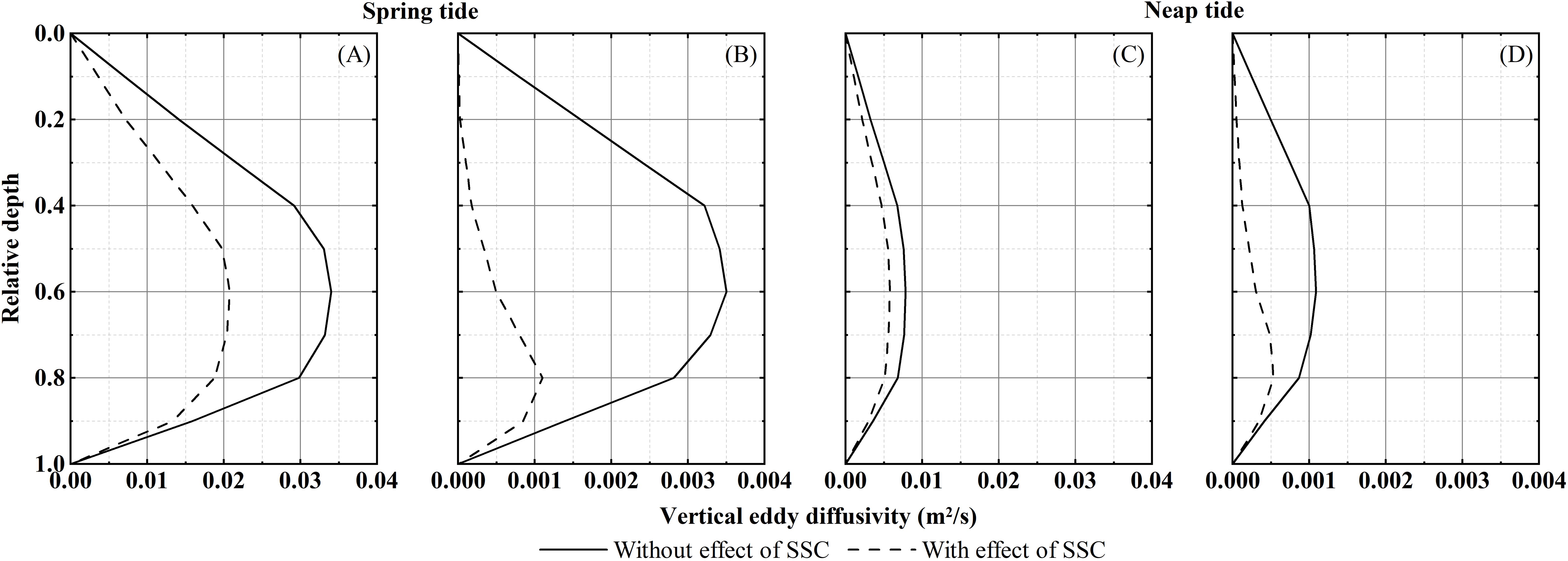
Figure 15. Variations in vertical eddy viscosity coefficient during flood tide at Section 12 induced by SSC (spring tide, Q = 1000 m³/s). (A) Peak flood (Spring tide); (B) Flood slack (Spring tide); (C) Peak flood (Neap tide); (D) Flood slack (Neap tide).

$\begin{array}{ll}\text{N}=({\rho }_b-{\rho }_t)/{\rho }_{ave}& (7)\end{array}$

where ${\rho }_b$ and ${\rho }_t$ represent the density of the surface and bottom layers, and ${\rho }_{ave}$ is the vertically averaged density.

As shown in Table 4, the tidal average density difference induced by SSC initially increases and then decreases as Q increases, consistent with the pattern of SSC variation with Q. Due to the reduction in salinity simulation results induced by SSC, the values of tidal-averaged density differences are slightly smaller than the values of the $\overline{\text{SSC}}$. It is also observed that the contribution of SSC to depth-averaged density increases with higher Q or further upstream. It’s mainly because salinity generally decreases with increasing Q or further upstream, leading to a diminishing influence on density compared to that of SSC. When the Q exceeds 1000 m³/s, the contribution of SSC to depth-averaged density between Laoyancang and Qibao (sections 10-14) generally exceeds 70%, significantly surpassing that of salinity.

The vertical density distribution of Section 12 at flood and ebb slack, as well as at flood and ebb peak, during the spring tide under annual average runoff (Q=1000 m³/s) is presented in Figure 14. It’s evident from Figure 14 that SSC can markedly increases both the magnitude and the vertical gradient of density at Section 12. When considering the impact of SSC, the N values at peak flood and flood slack rise from 4.68×10^-5 and 8.05×10^-5 to 4.68×10^-3and 4.68×10^-3 respectively, representing an increase of over 40 times. The vertical density gradient and N values are higher during the flood tide than the ebb tide, indicating that SSC’s contribution to density stratification is more pronounced during the flood tide. It’s primarily because the SSC is higher during the flood tide.

The Variations in the vertical density gradient induced by SSC will influence the vertical turbulent structure in the water column. As shown in Figure 15, the increase in vertical density gradient and stratification due to SSC reduce the vertical eddy diffusion coefficient values during the flood tide, indicating that vertical mixing is inhibited, which also weakens the turbulent diffusion of salinity. During the spring tide, the vertical eddy diffusion coefficient is reduced by 40-50% at peak flood, and by 70-90% at flood slack. This is mainly because the SSC and the vertical density gradient are greater at flood slack than at peak flood. The reduction in value of the vertical eddy diffusion coefficient due to SSC is more pronounced during the spring tide, because SSC values during the spring tide are higher compared to the neap tide, as well as its impact on fluid density is more significant than that of salinity.

4.3 Influence of SSC on flood tide hydrodynamics

The upstream movement of saltwater depends on flood tide hydrodynamics. Therefore, the variation of hydrodynamic factors (water level and current velocity) induced by SSC during flood tide directly influences the driving conditions for salinity transport and affects the simulation results of saltwater intrusion. To analyze the impact of SSC on hydrodynamic factors, we selected simulation results for Sections 10, 12 and 14 under dry season runoff (Q = 500 m³/s) and calculated the difference of cross-sectional average water level, velocity, and salinity (ΔH, ΔV and ΔS, ΔH = H₀ - H_C, ΔV = V₀ - V_C, ΔS = S_C - S_C) induced by SSC in a whole spring tide period, as shown in Figure 16.

Figure 16

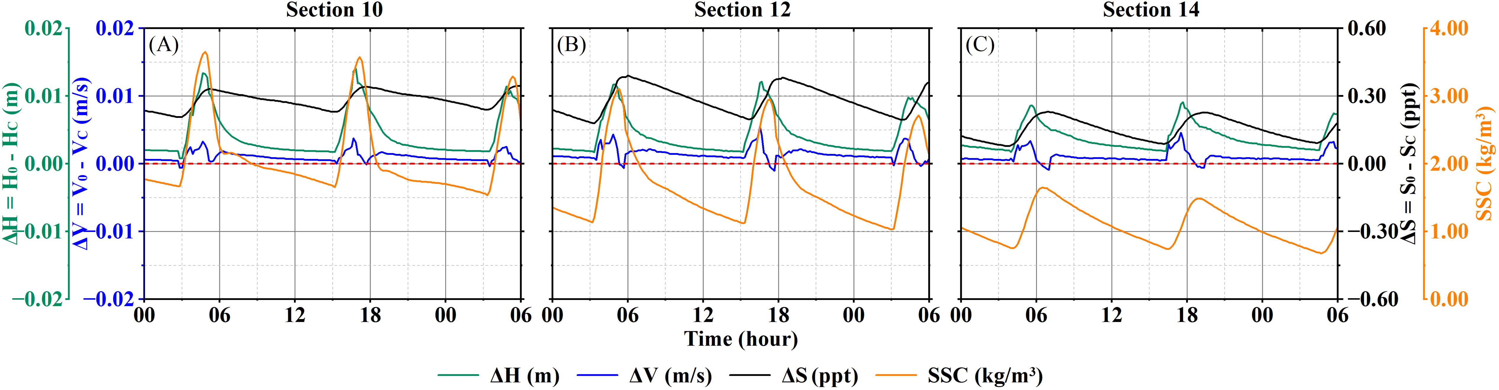
Figure 16. The temporal variations of ΔS and SSC in Section 10-14 when considering the impact of SSC. (Q = 500m³/s, Spring tide).

It can be observed from Figure 16 that, except for salinity, the water level and velocity of three sections during flood tides also generally decrease when considering the impact of SSC. And as the SSC increases, the values of ΔH, ΔV and ΔS also increase accordingly. Sections 10, 12, and 14 exhibit maximum ΔH values of 1.41, 1.20, and 0.91 cm, maximum ΔV values of 0.38, 0.54, and 0.46 cm/s, and maximum ΔS values of 0.37, 0.40, and 0.24 ppt, respectively. The peaks of ΔH and ΔV are close to the high tide time, preceding the SSC peak by approximately 10-15 minutes, while the peak of ΔS lags the SSC peak by 10-20 minutes. The peaks of ΔH, ΔV, ΔS and SSC occur relatively close together in time.

Furthermore, we selected the ΔH, ΔV and ΔS series of three sections during flood tide and calculated the correlation coefficients between these three factors and SSC, as shown in Figure 17. According to Figure 17 that ΔH and ΔS exhibit a strong positive correlation with SSC, with R² ranging from 0.76 to 0.93, most of which are greater than 0.85. Except for Section 10, the correlation between ΔV and SSC during the flood tide is relatively weak (R² < 0.75), but overall, there is a clear trend of ΔV increasing with SSC. In general, ΔH, ΔV and ΔS in Sections 10-14 have strong positive correlations with SSC, and their peaks are close to the peak of SSC.

Figure 17

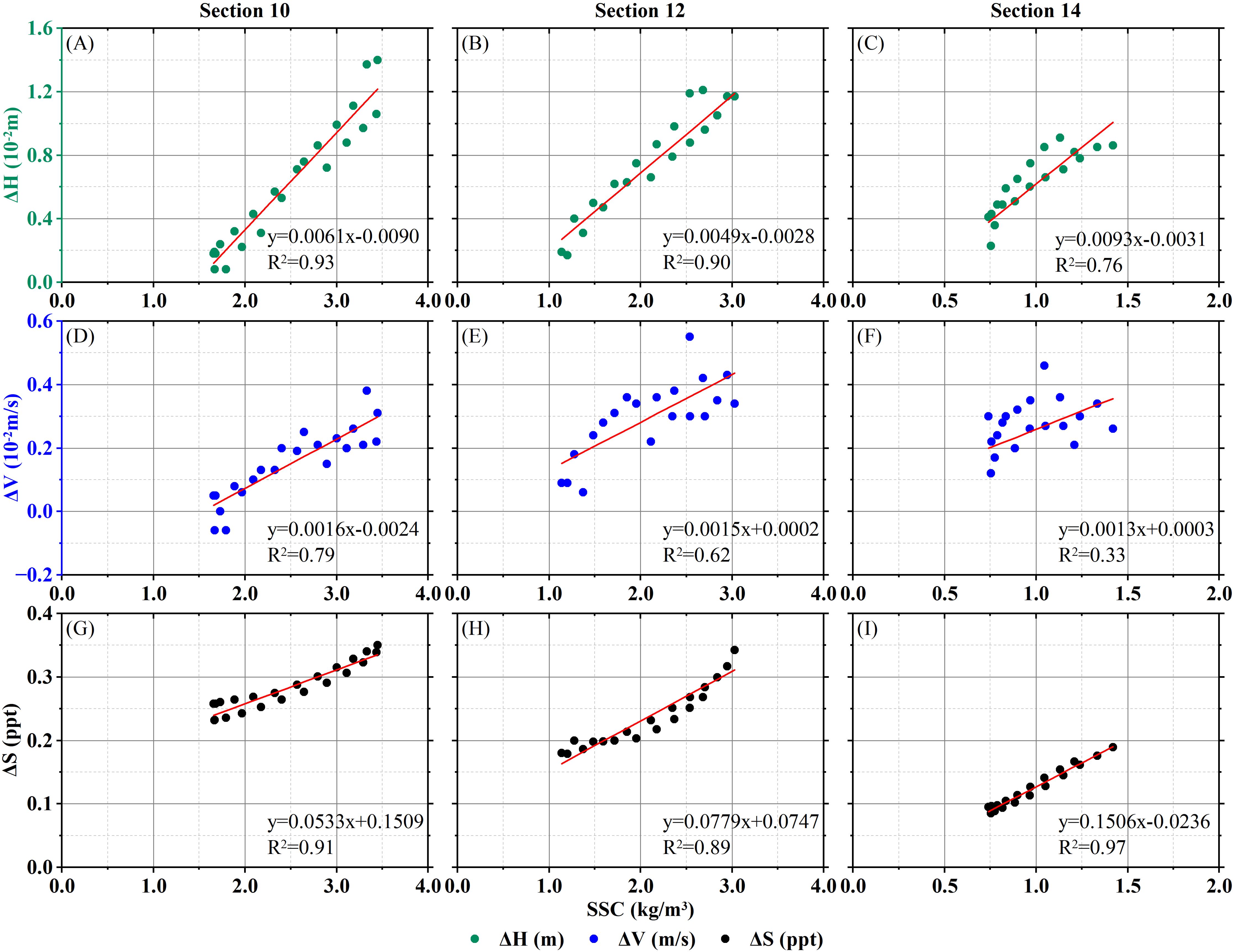
Figure 17. Relationship between ΔH, ΔV, ΔS and SSC in Sections 10-14 during flood tide. (A-C) ΔH and SSC; (D-F) ΔV and SSC; (G-I) ΔS and SSC.

4.4 Influence of SSC on salinity flux

To further investigate the impact of SSC on salinity transport in the Qiantang Estuary, we analyzed the changes in salinity flux induced by SSC during spring tide under dry season runoff (Q = 500 m³/s). Based on the simulation results from Sections 10-14, we calculated the average salinity flux generated by advective and dispersive transport during the flood tide at each cross-section, as shown in Table 5.

Table 5

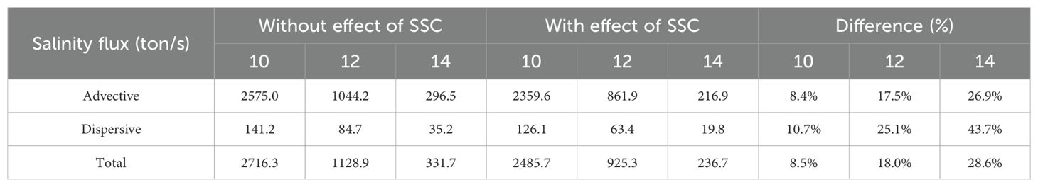
Table 5. Changes in average salinity flux induced by SSC (Spring Tide, Q=500 m³/s).

As can be seen from Table 5, the average salinity flux at each Section during the flood tide all decrease due to the impact of SSC, with the reduction degree becoming more pronounced upstream, which is consistent with the changes in ΔS%. During the spring tide, the average total salinity flux at Sections 10, 12, and 14 decreased by 230.5, 203.6, and 95.0 tons/s, respectively, corresponding to reductions of 8.5%, 17.9%, and 28.6%.

Comparing the proportions of salinity flux contributed by advection and dispersion to the total salinity flux during the flood tide in Section 10-14, the advective transport is the primary mode for salinity transport in this region, accounting for over 90% of the total flux. However, the proportion of dispersive transport increases upstream, rising from 5.1% to 8.0%, which indicates that advection-driven salinity transport weakens while dispersion-driven transport strengthens when moving upstream. The results reveal that both the advective and dispersive salinity flux decrease when considering the density effect of SSC, which is primarily due to the reduced flood tide velocity and turbulence diffusion. Moreover, the influence of SSC on dispersive salinity flux is more significant than on advective salinity flux, with this impact becoming more pronounced upstream. At Section 14, the reduction in dispersive salinity flux can reach up to twice as much as that of advective salinity flux.

4.5 Mechanism of SSC influencing saltwater intrusion

In Sections 4.2 to 4.4, we explored the impact of SSC on density distribution, turbulent diffusion, tidal hydrodynamics, and salinity flux. Based on the above analysis, we attempted a preliminary investigation of the mechanism by which SSC influences saltwater intrusion.

During the process of saltwater intrusion, salinity transport primarily depends on advection and diffusion, both of which are weakened by the density effect of SSC. Advective transport is the dominant mode of salinity transport in the Qiantang Estuary, and the reduction in advective salinity flux is mainly due to two reasons. First, the value of water density generally increases when considering the SSC’s effect on density. As sediment-laden water moves upstream during flood tides, it requires more kinetic energy to be converted into potential energy, leading to a reduction in flood current velocity and water level, and thus diminishing the driving force for saltwater moving upstream. In the Qiantang Estuary, the bed level exhibits an overall trend of first rising and then falling from Ganpu to Wenyan, with the top of the underwater sandbar located near Cangqian (Xie et al., 2018). It explains why ΔS first increases and then decreases as it moves upstream, with the location of ΔS peak aligning with the sandbar top. Second, driven by the increasing current velocity during flood tide, a great amount of sediment is suspended and moves upstream with flood flow, causing a continuous rise in SSC until it peaks near the flood slack moment. The increasing SSC during the flood tide increases the energy required to maintain suspension. Therefore, ΔH and ΔV in Sections 10-14 show a strong positive correlation with SSC, both increasing with SSC during flood tide (Figure 10). Additionally, the weakened salinity transport lowers salinity levels in the upstream reach. The diminished upstream salinity combines with the decrease in flood discharge caused by the reduced flood current velocity and water level, which amplifies the decrease in advective salinity flux. This effect accumulates from the Ganpu boundary to the upstream, resulting in ΔS initially increasing before gradually decreasing due to the rapid decrease in salinity upstream. The reduction in dispersive salinity flux is basically related to the weakening of turbulence and mixing caused by SSC-induced density stratification. As analyzed in Section 6.1, an increase in the relative influence of SSC on water density leads to a decrease in vertical eddy diffusivity. Given that SSC’s contribution to water density increases upstream between Sections 10 and 14 (Table 4), the suppression of turbulent diffusion becomes more pronounced, characterized by a greater reduction in dispersive salinity flux.

In summary, SSC causes both the magnitude and vertical gradient of density during flood tides, which in turn increases the energy required for sediment-laden water to move upstream, leading to a reduction in current velocity, water level, and vertical turbulent diffusion during flood tides. It weakens the driving force for saltwater moving or spreading upstream, reducing both advective and diffusive upstream transport of salinity, represented by the decrease of the upstream salinity value, that is, the inhibition of saltwater intrusion. Therefore, it is crucial to account for the impact of SSC on fluid density when simulating salinity in estuaries with high SSC. It can ensure a more accurate simulation of hydrodynamic conditions, thereby improving the accuracy and reliability of salinity simulation results.

5 Conclusion

This paper established a new 3D baroclinic model coupling flow, salinity and SSC based on Delft3D to simulate the salinity distribution in the Qiantang Estuary. By analyzing the changes of salinity simulation results induced by SSC, the following conclusions were drawn:

1. Both the measured data and the numerical simulation results show that the impact of SSC on fluid density is generally greater than that of salinity between Yanguan and Qibao, especially when the Q exceeds 1000 m³/s. Therefore, the density effect of SSC cannot be ignored in numerical simulations of salinity in the Qiantang Estuary.

2. Simulation results under different runoff and tidal conditions indicated that simulated salinity values generally decreases and contours move downstream when considering the impact of SSC, suggesting a weakening effect on saltwater intrusion. The salinity difference (ΔS) caused by SSC initially increases and then decreases from Ganpu to Wenyan, with a maximum value of 0.41 ppt and occurring during spring tide when Q is 500 m³/s, located at 78km upstream of Ganpu. And the saltwater intrusion distance is reduced by a maximum of 6.4km at the same time. As downstream tidal range decreases or upstream Q increases, the ΔS peak decreases and shifts downstream. When Q exceeds 3000 m³/s, ΔS is generally less than 0.03 ppt, and the effect of SSC on salinity simulation results can be ignored.

3. The distribution of ΔS and SSC shows a strong spatio-temporal correlation. From Laoyancang to Qibao (Sections 10-14), the ΔS peaks only lag the SSC peaks by approximately 10-20 minutes, and the ΔS exhibit a positive correlation with SSC during flood tides, with correlation coefficients reaching 0.89-0.97. The peak locations of $\text{Δ}\overline{\text{S}}$ and $\overline{\text{SSC}}$ are relatively close, essentially coinciding under annual average runoff (Q = 1000 m³/s).

4. A preliminary exploration of the mechanism by which SSC influences saltwater intrusion is conducted by discussing its impact on density stratification, flood tide hydrodynamics, and salinity flux. Analysis of simulation results between Laoyancang and Qibao reveals that the density effect of SSC will decrease tidal level, current velocity, and vertical eddy diffusion coefficient during flood tide, and increase the vertical density gradient, ultimately decreasing both advective and diffusive salinity fluxes. A positive correlation exists between ΔH, ΔV, and SSC during flood tides, meanwhile, the higher SSC enhance density stratification and inhibits vertical mixing. It indicates that SSC will weaken the driving force for saltwater intrusion, reduce both advective and diffusive upstream transport of salinity, and thereby resulting in a decrease in estuarian salinity simulation results. Therefore, considering the impact of SSC on fluid density is crucial for accurately simulating salinity in estuaries with high SSC, particularly under low-flow and high-tide conditions.

Although this study has conducted a numerical investigation on the impact of SSC on salinity distribution simulation in a high SSC estuary and preliminarily discussed the mechanism of SSC influencing saltwater intrusion, further research is still needed to fully understand the mechanisms by which SSC affects salinity transport, especially its influence on the conversion of potential and kinetic energy and turbulent energy dissipation during flood tides. Additionally, in the Qiantang Estuary, vertical mixing is relatively strong, and vertical stratification of salinity and SSC is not significant. Therefore, in the next phase of our research, we will continue to investigate the impact of SSC on salinity transport in partially mixed or weakly mixed high-turbidity estuaries and compare these findings with those from well-mixed estuaries. And we will also conduct relevant idealized numerical models and physical flume experiments to further explore how different SSC levels influence salinity advective and diffusive transport of salinity in the estuaries.

Data availability statement

The original contributions presented in the study are included in the article/supplementary material. Further inquiries can be directed to the corresponding author.

Author contributions

ZR: Data curation, Methodology, Software, Visualization, Writing – original draft. HC: Supervision, Writing – review & editing. SZ: Supervision, Writing – review & editing. SY: Writing – review & editing.

Funding

The author(s) declare financial support was received for the research, authorship, and/or publication of this article. This work was supported by the Zhejiang Provincial Department of Science and Technology (No. 2023C03119), the National Natural Science Foundation of China (No. 91647209), and the Joint Fund Project of Zhejiang Provincial Natural Science Foundation (No. LZJWY24E090001).

Conflict of interest

The authors declare that the research was conducted in the absence of any commercial or financial relationships that could be construed as a potential conflict of interest.

Publisher’s note

All claims expressed in this article are solely those of the authors and do not necessarily represent those of their affiliated organizations, or those of the publisher, the editors and the reviewers. Any product that may be evaluated in this article, or claim that may be made by its manufacturer, is not guaranteed or endorsed by the publisher.

References

Akter A., Tanim A. H. (2021). Salinity distributio17n in river network of a partially mixed estuary. J. Waterw. Port. Coast. Ocean. Eng. 147, 04020055. doi: 10.1061/(ASCE)WW.1943-5460.0000621

Crossref Full Text | Google Scholar

Álvarez A. H., Otero L., Restrepo J. C., Álvarez O. (2022). The effect of waves in hydrodynamics, stratification, and salt wedge intrusion in a microtidal estuary. Front. Mar. Sci. 9. doi: 10.3389/fmars.2022.974163

PubMed Abstract | Crossref Full Text | Google Scholar

Bellafiore D., Ferrarin C., Maicu F., Manfè G., Lorenzetti G., Umgiesser G., et al. (2021). Saltwater intrusion in a mediterranean delta under a changing climate. J. Geophys. Res. 126, e2020JC016437. doi: 10.1029/2020JC016437

Crossref Full Text | Google Scholar

Brice L., Niño C. Y., Escauriaza M. C. (2005). Finite volume modeling of variable density shallow-water flow equations for a well-mixed estuary: application to the Río Maipo estuary in central Chile. J. Hydraulic. Res. 43, 339–350. doi: 10.1080/00221680509500130

Crossref Full Text | Google Scholar

Bricheno L. M., Wolf J., Sun Y. (2021). Saline intrusion in the Ganges-Brahmaputra-Meghna megadelta. Estuar. Coast. Shelf. Sci. 252, 107246. doi: 10.1016/j.ecss.2021.107246

Crossref Full Text | Google Scholar

Cancino L., Neves R. (1999). Hydrodynamic and sediment suspension modelling in estuarine systems Part I: Description of the numerical models. J. Mar. Syst. 22, 105–116. doi: 10.1016/S0924-7963(99)00035-4

Crossref Full Text | Google Scholar

Chen L., Gong W., Zhang H., Zhu L., Cheng W. (2020). Lateral circulation and associated sediment transport in a convergent estuary. JGR. Oceans. 125, e2019JC015926. doi: 10.1029/2019JC015926

Crossref Full Text | Google Scholar

Chen J., Liu C., Zang C., Walker H. J. (1990). Geomorphological development and sedimentation in qiantang estuary and hangzhou bay. J. Coast. Res. 6, 559–572. Available at: https://www.jstor.org/stable/4297719.

Google Scholar

Chen Y., Zuo J., Zou H., Zhang M., Zhang K. (2016). Responses of estuarine salinity and transport processes to sea level rise in the Zhujiang (Pearl River) Estuary. Acta Oceanol. Sin. 35, 38–48. doi: 10.1007/s13131-016-0857-2

Crossref Full Text | Google Scholar

Gao Y., Wang X., Dong C., Ren J., Zhang Q., Huang Y. (2024). Characteristics and influencing factors of storm surge-induced salinity augmentation in the pearl river estuary, South China. Sustainbility 16, 2254. doi: 10.3390/su16062254

Crossref Full Text | Google Scholar

Guillou N., Chapalain G., Petton S. (2023). Predicting sea surface salinity in a tidal estuary with machine learning. Oceanologia 65, 318–332. doi: 10.1016/j.oceano.2022.07.007

Crossref Full Text | Google Scholar

Guo Y., Wu X., Pan C., Zhang J. (2012). Numerical simulation of the tidal flow and suspended sediment transport in the qiantang estuary. J. Waterway. Port. Coastal. Ocean. Eng. 138, 192–202. doi: 10.1061/(ASCE)WW.1943-5460.0000118

Crossref Full Text | Google Scholar

Han Z., Cheng H., Shi Y., You A. (2012). Long-term predictions and countermeasures of saltwater intrusion in the Qiantang estuary. J. Hydraulic. Eng. 43, 232–240.

Google Scholar

Han Z., Pan C., Yu J., Chen H. (2001). Effect of large-scale reservoir and river regulation/reclamation on saltwater intrusion in Qiantang Estuary. Sc. China Ser. B-Chem. 44, 221–229. doi: 10.1007/BF02884830

Crossref Full Text | Google Scholar

Hu J., Liu B., Peng S. (2019). Forecasting salinity time series using RF and ELM approaches coupled with decomposition techniques. Stoch. Environ. Res. Risk Assess. 33, 1117–1135. doi: 10.1007/s00477-019-01691-1

Crossref Full Text | Google Scholar

Huang J., Sun Z., Xie D. (2022). Morphological evolution of a large sand bar in the Qiantang River Estuary of China since the 1960s. Acta Oceanol. Sin. 41, 156–165. doi: 10.1007/s13131-021-1817-z

Crossref Full Text | Google Scholar

Jeong J.-S., Woo S.-B., Lee H. S., Gu B.-H., Kim J. W., Song J. I. (2022). Baroclinic effect on inner-port circulation in a macro-tidal estuary: A case study of incheon North Port, Korea. JMSE 10, 392. doi: 10.3390/jmse10030392

Crossref Full Text | Google Scholar

Jiao J., Huang S., Zheng R. (2021). Influence of tide and runoff on saltwater intrusion in the qiantang river estuary, China. IOP. Conf. Ser.: Earth Environ. Sci. 691, 12014. doi: 10.1088/1755-1315/691/1/012014

Crossref Full Text | Google Scholar

Jones N. L., Monismith S. G. (2008). The influence of whitecapping waves on the vertical structure of turbulence in a shallow estuarine embayment. J. Phys. Oceanogr. 38, 1563–1580. doi: 10.1175/2007JPO3766.1

Crossref Full Text | Google Scholar

Li R., Gao L., Pan C., Pang Y. (2019). Detecting the mechanisms of longitudinal salt transport during spring tides in Qiantang Estuary. J. Integr. Environ. Sci. 16, 123–140. doi: 10.1080/1943815X.2019.1652190

Crossref Full Text | Google Scholar

Li R., Pan C., Ge C., Wu X. (2020). Analysis and numerical simulation of the limiting factors of algal blooms in Qiantang River estuary. IOP. Conf. Ser.: Earth Environ. Sci. 569, 12080. doi: 10.1088/1755-1315/569/1/012080

Crossref Full Text | Google Scholar

Lu T., Wu H., Zhang F., Li J., Zhou L., Jia J., et al. (2020). Constraints of salinity- and sediment-induced stratification on the turbidity maximum in a tidal estuary. Geo-Mar. Lett. 40, 765–779. doi: 10.1007/s00367-020-00670-8

Crossref Full Text | Google Scholar

Moseev D. S., Leshchev A. V., Sergienko L. A., Miskevich V., Makhnovich N. M., Lokhov A. S. (2022). Littoral phytocenoses of marshes located in different tidal conditions of the White Sea. Czech. Polar. Rep. 12, 181–202. doi: 10.5817/CPR2022-2-14

Crossref Full Text | Google Scholar

Niroomandi A., Ma G., Su S.-F., Gu F., Qi D. (2018). Sediment flux and sediment-induced stratification in the Changjiang Estuary. J. Mar. Sci. Technol. 23, 349–363. doi: 10.1007/s00773-017-0478-2

Crossref Full Text | Google Scholar

Pan C., Huang W. (2010). Numerical modeling of suspended sediment transport affected by tidal bore in qiantang estuary. J. Coast. Res. 26, 1123–1132. doi: 10.2112/JCOASTRES-D-09-00024.1

Crossref Full Text | Google Scholar

Pan C., Zhang S., Shi Y., Lu H., Xie D. (2014). Study on saltwater intrusion in Qiantang estuary affected by tidal bore. J. Hydraulic. Eng. 45, 1301–1309.

Google Scholar

Partheniades E. A. (1965). Erosion and deposition of cohesive soils. J. Hydraulic. Eng. 91, 105–139. doi: 10.1061/JYCEAJ.0001165

Crossref Full Text | Google Scholar

Qin H., Shi H., Gai Y., Qiao S., Li Q. (2023). Sensitivity analysis of runoff and wind with respect to yellow river estuary salinity plume based on FVCOM. Water 15, 1378. doi: 10.3390/w15071378

Crossref Full Text | Google Scholar

Rodrigues M., Fortunato A. B. (2017). Assessment of a three-dimensional baroclinic circulation model of the Tagus estuary (Portugal). AIMS. Environ. Sci. 4, 763–787. doi: 10.3934/environsci.2017.6.763

Crossref Full Text | Google Scholar

Shen Q., Huang W., Wan Y., Gu F., Qi D. (2020). Observation of the sediment trapping during flood season in the deep-water navigational channel of the Changjiang Estuary, China. Estuar. Coast. Shelf. Sci. 237, 106632. doi: 10.1016/j.ecss.2020.106632

Crossref Full Text | Google Scholar

Shi H., Li Q., Sun J., Gao G., Sui Y., Qiao S., et al. (2020). Variation of yellow river runoff and its influence on salinity in laizhou bay. J. OCEAN. Univ. 19, 1235–1244. doi: 10.1007/s11802-020-4413-5

Crossref Full Text | Google Scholar

Stanev E. V., Jacob B., Pein J. (2019). German Bight estuaries: An inter-comparison on the basis of numerical modeling. Continental. Shelf. Res. 174, 48–65. doi: 10.1016/j.csr.2019.01.001

Crossref Full Text | Google Scholar

Sun Z., Yang E., Xu D., Ni X. (2018). Logarithmic law for transport capacity of nonuniform sediment. J. Hydraul. Eng. 144, 04017069. doi: 10.1061/(ASCE)HY.1943-7900.0001390

Crossref Full Text | Google Scholar

Telesh I. V., Khlebovich V. V. (2010). Principal processes within the estuarine salinity gradient: A review. Mar. pollut. Bull. 61, 149–155. doi: 10.1016/j.marpolbul.2010.02.008

PubMed Abstract | Crossref Full Text | Google Scholar

Wan Y., Wang L. (2017). Numerical investigation of the factors influencing the vertical profiles of current, salinity, and SSC within a turbidity maximum zone. Int. J. Sediment. Res. 32, 20–33. doi: 10.1016/j.ijsrc.2016.07.003

Crossref Full Text | Google Scholar

Wan Y., Wu H., Roelvink D., Gu F. (2015). Experimental study on fall velocity of fine sediment in the Yangtze Estuary, China. Ocean. Eng. 103, 180–187. doi: 10.1016/j.oceaneng.2015.04.076

Crossref Full Text | Google Scholar

Wang Q., Fellow P. (2018). Three-dimensional modelling of sediment transport under tidal bores in the Qiantang estuary, China. J. Hydraulic. Res. 56, 662–672. doi: 10.1080/00221686.2017.1397781

Crossref Full Text | Google Scholar

Wang Q., Pan C. (2018). Three-dimensional modelling of sediment transport under tidal bores in the Qiantang estuary, China. J. Hydraulic. Res. 56, 662–672. doi: 10.1080/00221686.2017.1397781

Crossref Full Text | Google Scholar

Weng X., Jiang C., Zhang M., Yuan M., Zeng T. (2020). Numeric study on the influence of sluice-gate operation on salinity, nutrients and organisms in the jiaojiang river estuary, China. Water 12, 2026. doi: 10.3390/w12072026

Crossref Full Text | Google Scholar

Winterwerp J. C. (2001). Stratification effects by cohesive and noncohesive sediment. J. Geophys. Res.-Oceans. 106, 22559–22574. doi: 10.1029/2000JC000435

Crossref Full Text | Google Scholar

Winterwerp J. C. (2006). Stratification effects by fine suspended sediment at low, medium, and very high concentrations. J. Geophys. Res.-Oceans. 111, C05012. doi: 10.1029/2005JC003019

Crossref Full Text | Google Scholar

Wu R., Li J., Liu Q., Jin Y., Liu Q. (2007). Study on flocculation and setting characteristics of cohesive fine grain sediment in the Qiantang Estuary. Trans. Oceanol. Limnol., 24–34.

Google Scholar

Wu H., Tu X., Chen X., Vijay P. S., Leonardo A., Lin K., et al. (2023). A framework for water supply regulation in coastal areas by avoiding saltwater withdrawal considering upstream streamflow distribution. Sci. Total. Environ. 905, 167181. doi: 10.1016/j.scitotenv.2023.167181

PubMed Abstract | Crossref Full Text | Google Scholar

Xie D., Huang J., Bo J., Li R., Tang Z., Lu H. (2020). “A preliminary study on seasonal variations of sediment concentrations in the inner Qiantang Estuary,” in 2020 THIRD INTERNATIONAL WORKSHOP ON ENVIRONMENT AND GEOSCIENCE. Eds. Xu Z., Peng X. (IoP Publishing Ltd, Bristol), 012079. doi: 10.1088/1755-1315/569/1/012079

Crossref Full Text | Google Scholar

Xie D., Pan C., Gao S., Wang Z. B. (2018). Morphodynamics of the Qiantang Estuary, China: Controls of river flood events and tidal bores. Mar. Geol. 406, 27–33. doi: 10.1016/j.margeo.2018.09.003

Crossref Full Text | Google Scholar

Xu D., Sun Z. L., Zhu L., Huang S. (2013). Numerical simulation of salinity in qiantang river estuary. Oceanol. Limnol. Sin. 44, 829–836.

Google Scholar

Yu Q., Wang Y., Gao J., Gao S., Flemming B. (2014). Turbidity maximum formation in a well-mixed macrotidal estuary: The role of tidal pumping. J. Geophys. Res. Oceans. 119, 7705–7724. doi: 10.1002/2014JC010228

Crossref Full Text | Google Scholar

Zhao L., Xin P., Cheng H., Chu A. (2022). Combined effects of river discharge regulation and estuarine morphological evolution on salinity dynamics in Yangtze Estuary, China. Estuar. Coast. Shelf. Sci. 276, 108002. doi: 10.1016/j.ecss.2022.108002

Crossref Full Text | Google Scholar

Zhou J., Stacey M. T., Holleman R. C., Nuss E., Senn D. B. (2020). Numerical investigation of baroclinic channel-shoal interaction in partially stratified estuaries. JGR. Oceans. 125, e2020JC016135. doi: 10.1029/2020JC016135

Crossref Full Text | Google Scholar

Zhu C., van Maren D. S., Guo L., Lin J., He Q., Wang Z. B. (2021). Effects of sediment-induced density gradients on the estuarine turbidity maximum in the yangtze estuary. J. Geophys. Res.-Oceans. 126, e2020JC016927. doi: 10.1029/2020JC016927

Crossref Full Text | Google Scholar