Revisiting Thorpe scale analysis and diapycnal diffusivities in Drake Passage

Ship heave effects in the swell-prevalent Southern Ocean induce frequent false overturns in density profiles, and conventional Thorpe scale analysis leads to unrealistically large diapycnal diffusivities. Another critical factor causing large positive biases in Thorpe scale analysis concerns the Ozmidov to Thorpe scales ratio α often considered constant and equal to 0.8. A revised Thorpe scale analysis is proposed with an innovative segment-by-segment approach to circumvent heave-induced false overturns together with best-fitting α functions to Diapycnal and Isopycnal Mixing Experiment in the Southern Ocean (DIMES) data, which yields realistic diffusivities in the Drake Passage region. The revised Thorpe scale method applied to a finely-resolved CTD section across the Drake Passage yields typical diffusivities of O (10^-5-10^-3 m² s^-1), with the largest values being preferentially concentrated close to the bottom at major circumpolar fronts, consistent with nearby DIMES microstructure observations. In the southern Drake Passage the method highlights a middepth (500-1500 m) mixing maximum of 10^-4-10^-3 m² s^-1 in the Lower Circumpolar Deep Water (LCDW) layer due to large intrusions of Warm Deep Water (a cold/fresh variety of LCDW) of Weddell Gyre origin. The inferred middepth mixing maximum in intrusive regions, which is associated with isopycnal eddy stirring rather than caused by internal waves or double diffusive mixing, supports the short-circuiting paradigm of meridional overturning circulation in the southwestern Scotia Sea region and has important climatic implications in a warming climate.

1 Introduction

Diapycnal mixing controls the abyssal stratification and upwelling of deep waters originating from convectively-sunken cold polar waters. It is a key parameter for the meridional overturning circulation of the global ocean. Munk (1966) diagnosed that a diapycnal diffusivity of 10^-4 m² s^-1 is needed to maintain the abyssal stratification. Using a global dataset of microstructure measurements, Waterhouse et al. (2014) found that the depth-averaged global diapycnal diffusivity below 1000-m depth is O (10^-4 m² s^-1), consistent with Munk (1996). However, direct turbulence measurements from microstructure profilers are much too demanding in cost and in-situ operations, so they are very sparse in the global ocean (Waterhouse et al., 2014), especially considering the strong intermittency and spatial heterogeneity of turbulent mixing. In the Southern Ocean, microstructure measurements of the turbulent kinetic energy dissipation rate ε have been mostly restricted to the Kerguelen region (Waterman et al., 2013) and the southeast Pacific and Drake Passage region in particular during the Diapycnal and Isopycnal Mixing Experiment in the Southern Ocean (DIMES) surveys (Ledwell et al., 2011; St. Laurent et al., 2012; Sheen et al., 2013). Therefore, the use of more accessible indirect methods (detailed below) for inferring diapycnal diffusivities to fill gaps of direct measurements is all the more pressing, especially in the remote and harsh conditions of the Southern Ocean. In particular, there are no microstructure measurements of ε in the southwestern Scotia Sea region in the southern Drake Passage, where Naveira Garabato et al. (2007) suggested a “short-circuiting” of the meridional overturning circulation due to enhanced diapycnal mixing and upwelling of Circumpolar Deep Water (CDW). There is increasing interest on the weakening of the lower overturning cell in the Southern Ocean in association with volume contraction of Antarctic Bottom Water (AABW) and warming CDW (Chen et al., 2023; Lee et al., 2023). To better understand climatic implications of the Southern Ocean overturning circulation, a precise knowledge of diapycnal diffusivity and associated upwelling of CDW is primordial especially in the southern Drake Passage.

Osborn (1980) parameterized the diapycnal diffusivity K_ρ as a function of ε:

$\begin{array}{ll}{K}_{\rho }=\Gamma ϵ/N^2& (1)\end{array}$

where Γ represents the flux coefficient (or mixing efficiency) defined as the ratio of the vertical buoyancy flux to ε, and N² = -gρ_z/ρ₀ is a squared buoyancy frequency (g is gravity, ρ₀ is a reference density, and ρ_z is the vertical gradient of neutral density). Based on the turbulent energy balance between turbulent production, dissipation and loss to buoyancy, Osborn (1980) suggested an upper bound of the mixing efficiency as Γ = 0.2, which we adopt here.

Microstructure profilers directly estimate ε from measurements of centimeter-scale vertical shear u_z (ε = 7.5νu_z²), where ν is molecular viscosity (e.g., St. Laurent et al., 2012). The most widely-used indirect methods in the Southern Ocean are the shear/strain methods, which generally use standard Conductivity-Temperature-Depth (CTD) and lowered acoustic Doppler current profiler (LADCP) data (Polzin et al., 2002; Naveira Garabato et al., 2004; Sloyan, 2005; Kunze et al., 2006; Waterman et al., 2013). The shear/strain methods indirectly estimate ε in terms of the finescale shear/strain variance normalized by that of midlatitude internal wave fields well described by the Garett and Munk model (Gregg and Kunze, 1991; Kunze et al., 1992). According to Kunze et al. (2006), these methods are known to be sensitive to i) the instrument noise in abyssal waters, ii) the noise in the integrated shear-variance in the higher-wavenumber range, and iii) the choice of the shear-to-strain variance ratio which varies from 3 (Garett and Munk model) to more than 10 depending on ocean basins, depth, and stratification. Frants et al. (2013) reported an order of magnitude difference between CTD-based strain diffusivities and DIMES microstructure-based diffusivities in Drake Passage. A systematic near-bottom overestimation was also reported in the Kerguelen region (Waterman et al., 2014).

Thorpe scale analysis (Thorpe, 1977), another indirect method that is the main concern of the present study, has been widely used to calculate the turbulence scale not only in the ocean but also more recently in the atmosphere (Ko and Chun, 2022; He et al., 2024). The Thorpe scale L_T is defined as the root mean square (rms) of vertical displacements that would be necessary for generating a gravitationally stably-stratified profile from an unstably-stratified density profile (Dillon, 1982). Theoretically, ε can be expressed as a function of the Ozmidov scale L_O and N (Ozmidov, 1965):

$\begin{array}{ll}ϵ=L_o^2{N}^3.& (2)\end{array}$

Thorpe (1977) advanced an idea of a close connection between L_T and L_O, with the L_O to L_T ratio α (≡ L_O/L_T) close to unity in the stably-stratified ocean:

$\begin{array}{ll}{L}_O=\alpha L_T& (3)\end{array}$

Dillon (1982) suggested an ensemble-mean relationship between the two length scales of α = 0.8, although individual patchwise-mean ratios vary by a factor of 3, between 0.4 and 1.2, depending on observation sites and turbulence intensity (Dillon, 1982; Ferron et al., 1998; Mater et al., 2015). By combining Equations 2, 3, ε can be estimated as:

$\begin{array}{ll}ϵ={\alpha }^2{L}_T^2{N}^3.& (4)\end{array}$

Then, the Thorpe scale-derived diapynal diffusivity from Equation 1, using Equation 4 and Γ = 0.2, can be estimated as

$\begin{array}{ll}{K}_{\rho }=0.2{\alpha }^2{L}_T^{2}N.& (5)\end{array}$

As K_ρ is dependent on the square of L_T, the basic question is how to identify “real” overturns or density inversions and separate them from “false” overturns induced by instrumental noise and measurement errors. Several useful approaches for this purpose have been proposed (Galbraith and Kelley, 1996; Ferron et al., 1998; Gargett and Garner, 2008 (GG08 hereafter); Frants et al., 2013), which are discussed in the following section. The conventional Thorpe scale analysis of ship-lowered CTD density profiles in the Southern Ocean yielded highly-variable results compared to microstructure measurements, varying from a good agreement to a high bias by up to one to two orders of magnitude, depending on observation sites and times (Frants et al., 2013). Surprisingly, ship heave effects, which can cause systematic false overturns of a vertical scale of a few meters up to order 10 m in heavy swell, constituting thus the most serious measurement error, have attracted little attention. Here we propose a simple approach to overcome this fundamental shortcoming of the conventional Thorpe scale analysis especially in the swell-prevalent Southern Ocean.

Previous work has mostly used a constant L_O/L_T ratio of α = 0.8 according to Dillon (1982) (e.g., Thompson et al., 2007; Frants et al., 2013; Park et al., 2014). However, Mater et al. (2015) reported large positive biases in Thorpe-scale estimates of turbulence dissipation in the Luzon Strait by nearly an order of magnitude compared to microstructure observations for large-scale convective overturns, in which available potential energy is greater than turbulence kinetic energy. These authors experimentally demonstrated a clear tendency of decreasing α with increasing L_T, with median α values ranging from 1.3 to 0.4 depending on observation sites as well as intensity and age of turbulence; smaller (larger) α tends to be associated with “young” (“old”) turbulence characterized by large (small) L_T and higher (lower) available potential energy compared to turbulence kinetic energy.

In section 2, after discussing the CTD density noise issue, we present a revised Thorpe scale method using an innovative segment-by-segment approach to circumvent heave-induced false overturns, and assess this updated method using DIMES CTD and microstructure measurements in the Drake Passage region (St. Laurent et al., 2012). We perform a comparative study of K_ρ for different choices of α between the conventional constant value of 0.8 and best-fitting α functions to DIMES data. In section 3 we apply both the segment-by-segment approach and the best-fitting α functions to a finely-resolved CTD section carried out in 1996 across the Antarctic Circumpolar Current (ACC) in Drake Passage (Provost et al., 2011). Particular emphasis is put on the original finding of outstanding middepth mixing maximum in intrusive regions in the southern Drake Passage. Section 4 summarizes and discusses the major results, in particular the climatic implications of enhanced middepth mixing in the southern Drake Passage for the intensification and short-circuiting of the meridional overturning circulation in the southwestern Scotia Sea region.

2 Revised Thorpe scale analysis

In contrast to many hydrographic data analyses, which usually use the one-meter-mean CTD data publicly available in hydrographic data base, the Thorpe scale analysis needs raw CTD data. Indeed, raw data contain precious information on the CTD fall speed (FS), a critical parameter for identifying false overturns, and on small-scale turbulence of tens of centimeters in size that can be resolvable from standard high-precision 24-Hz CTD, albeit often excessively contaminated by high-frequency measurement errors. This calls for particular attention in the preliminary treatment of raw data before conducting a series of procedures necessary for the revised analysis. A flow chart (Figure 1) summarizes the procedure steps, highlighting differences between the revised and conventional analyses. Details of each procedure are presented below, emphasizing the relative efficiency of the revised method compared to the conventional one.

Figure 1

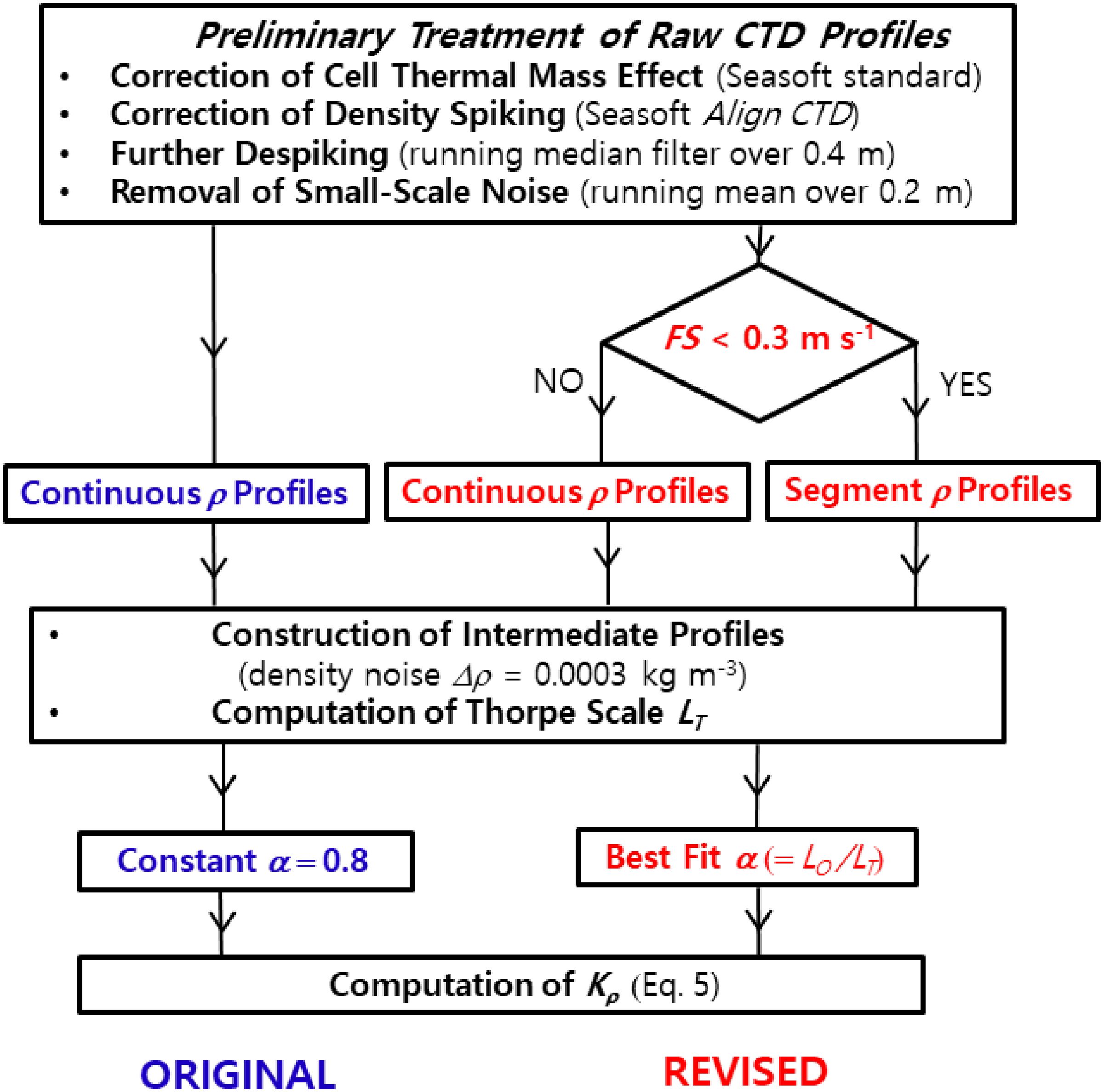
Figure 1. Flow chart of procedures employed in the revised Thorpe scale analysis. Parts specific to the revised (original or conventional) analysis are written in red (blue), while the common parts for both are in black. Segment profiles used in the revised analysis for suppressing heave-induced false overturns are constructed if the CTD fall speed (FS) drops below 0.3 m s^-1; otherwise, continuous profiles are used, much the same as in the conventional analysis. Another major difference between the two methods resides in the choice of the Ozmidov to Thorpe scales ratio α.

2.1 Preliminary treatment of raw CTD profiles

Spurious false density inversions leading to an unrealistic estimate of turbulence are caused by systematic measurement errors. We only used high-quality CTD profiles from standard Sea-Bird Electronics SBE 911plus or 9plus CTDs with a sampling frequency of 24 Hz, which yields a nominal vertical resolution of about 0.04 m with a typical CTD lowering speed of 1 m s^-1. Measurement errors causing spurious density inversions may largely result from the mismatch in time response of temperature and conductivity sensors or from a thermal inertia of conductivity cells. Galbraith and Kelley (1996) proposed a “water-mass test” measuring T-S tightness to identify and reject false overturns, whose practical application is not warranted by GG08. It is now common practice to process raw CTD data based on the Sea-Bird CTD data processing software Seasoft. For minimizing the measurement errors, raw CTD data are processed based on the Sea-Bird CTD data processing software (Seasoft V2 manual: SBE Data Processing, available at https://usermanual.wiki/Document/manualSeasoftDataProcessing7268.389551031.pdf). The instrumental density noise, which is independent of the raw data treatment, will be discussed later together with intermediate profiles used for computing Thorpe scales.

The raw CTD data were first corrected for the cell thermal mass effect according to the Seasoft standard, as this effect has no consequence for density spiking causing artificial overturns. The primary high-frequency measurement error in raw CTD data is salinity (and density) spiking caused by the misalignment of temperature and conductivity due to differing time responses of the temperature and conductivity sensors. The typical lag of conductivity relative to temperature is 0.073 s, which is commonly programmed in the deck unit to automatically advance conductivity on data acquisition at sea. This corresponds to the default case with zero correction in the Align CTD module. However, the default case is found out to be far from adequate for most CTD profiles from different cruises we have examined in the Southern Ocean, which calls for the search for an optimal advance of conductivity for each individual cruise. A visual inspection of selected density profiles recalculated with different time lags (incremented by ±0.01 s relative to the default case) permits to find an optimal lag yielding minimum density spiking (Figure 2A). The optimal lag correction is not constant but depends on each cruise: -0.04 s for the 2006 DRAKE cruise discussed in section 3; -0.05 s for the 2010 DIMES survey in the Drake Passage region discussed in subsections 2.4 and 3.1; a zero correction (default case) for the 2011 KEOPS II cruise in the Kerguelen region discussed in subsection 2.2. Note, however, that the results are practically insensitive for values within ±0.01 s around the optimal lags.

Figure 2

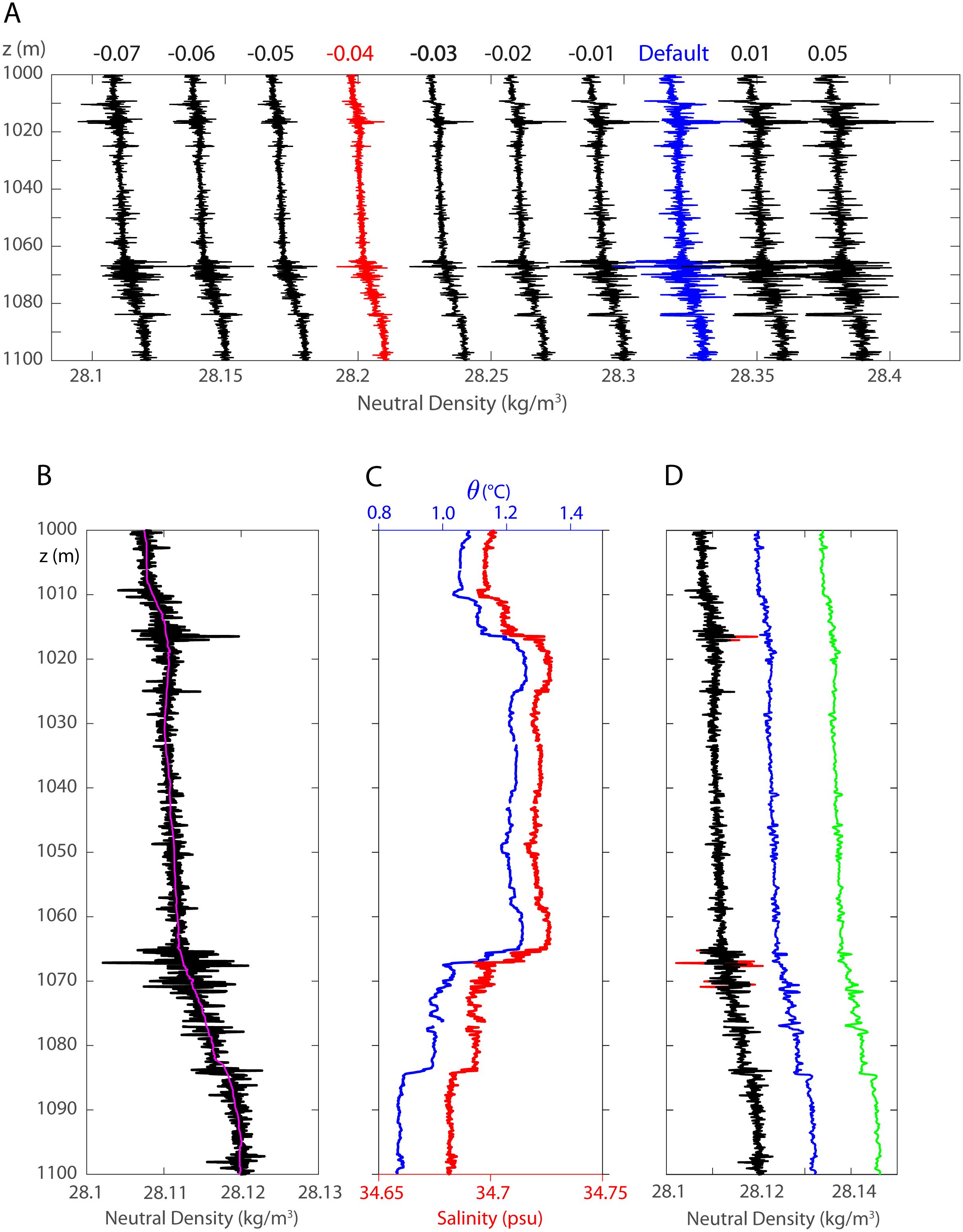
Figure 2. (A) Comparison of recalculated density profiles with different time lags (in second marked at the top line) for conductivity relative to the default case (zero lag, blue) using the Seasoft module Align CTD. The example is given for station 43 of the 2006 DRAKE cruise, which corresponds to one of the major intrusive regions in the southern Drake Passage discussed in subsection 3.3. The optimal profile (red) showing least density spiking can be seen for the correction with a lag of -0.04 sec. (B) Zoomed best lag-corrected density profile repeated from (A) (red profile). The magenta curve represents a larger-scale profile obtained using a 5-m running mean filter. (C) Corresponding potential temperature and salinity profiles showing steep gradients at intrusive levels centered at 1017 and 1067-m depth. (D) Outlier spikes exceeding 5 times the rms anomaly (red spikes) have been previously removed to have an intermediate profile (black), which is low-pass filtered with a 0.4-m running median filter at a regular 0.05-m depth interval to get a “spike-free” profile (blue). Finally, the latter de-spiked profile is further low-pass filtered using a 0.2-m running mean filter at a regular 0.1-m depth interval (green), which constitutes a final profile entered in the subsequent Thorpe scale analysis.

Even with the optimal lag correction of -0.04 s in Figure 2A for the DRAKE cruise, there still remain spurious high-frequency density spikes of vertical scales less than a few tens of centimeter, especially at depths around 1017 m and 1067 m (Figure 2B). The exact cause of such a feature is not known but might have been produced by amplification of imperfect lag correction over sharp temperature/salinity gradients especially in intrusive regions (Figure 2C). We wonder whether aliasing of imperfectly lag-corrected, unresolved small-scale turbulence might be a potential cause, although further precise analysis of the feature is needed. In order to suppress spurious spikes, we previously removed outliers surpassing 5-sigma noise level (Figure 2D, red spikes) relative to a larger-scale 5-m running-mean profile (magenta curve in Figure 2B). The resulting profile (black line in Figure 2D) was then low-pass filtered with a 0.4-m median filter at a 0.05-m depth interval to get a “spike-free” profile (blue line). Note that the chosen 0.05-m depth interval for the running median filter is close to the nominal vertical resolution of 0.04 m of raw CTD data. The “spike-free” profiles are then low-pass filtered with a 0.2-m running mean filter at a regular 0.1-m depth interval, suppressing small-scale random noise shorter than 0.2 m (green line), which constitute the final profiles used for the subsequent Thorpe scale analysis. We consider the latter value (0.2 m) as a minimum-resolvable L_T, and 3 times the latter (0.6 m) as a minimum resolvable overturn length. For a typical weak stratification in the deep Southern Ocean (N of order 10^-3 s^-1), the minimum resolvable L_T of 0.2 m yields a minimum resolvable diffusivity of 5 x 10^-6 m² s^-1 (Table 1), which can be also interpreted as a rough boundary between the residual noise and resolvable turbulence. Table 1 indicates that in order to detect at least the ambient diffusivity of order 1 x 10^-5 m² s^-1, L_T should be less than 0.3 m, although these parameters are close to their presumed noise level (5 x 10^-6 m² s^-1, 0.2 m). Note finally that the proposed raw-data treatment schemes are not confined to the revised Thorpe scale analysis but can be equally applicable to the conventional one.

Table 1

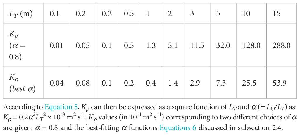
Table 1. Theoretical estimates of K_ρ for different L_T values using N = 10^-3 s^-1 that is typical in the deep Southern Ocean.

2.2 Heave-induced false overturns and an innovative segment-by-segment approach

Concerning ship heave effects, previous work did not take any special action, except for locating sections of pressure reversals and editing out data between successive encounters of the same pressure (GG08), or removing, via the Loop Edit module of Seasoft, all scans where the CTD descent rate is less than a chosen threshold value of 0.2 m s^-1 (Frants et al., 2013). These authors found that this Loop Edit correction had no effect on their diffusivity estimates and decided not to include it in their final analysis. In stark contrast to this, we show that the heave effects may constitute the principal source of systematic false overturns in the swell-prevalent Southern Ocean and propose an original approach to circumvent heave effects to estimate reliable diffusivities.

As a typical example of heave-induced false overturns, we show a zoomed 250-350-m segment of a processed density profile at a shallow plateau station (about 500 m deep) in the Kerguelen region (Park et al., 2014; Park et al., 2022) in Figure 3. The most noticeable features are abnormal negative density anomalies at three depths where the CTD fall speed FS drops below a threshold of 0.3 m s^-1 (marked by arrows in Figures 3A, B). These are believed to have been caused by the forward overshooting past the sensors of water entrained in the wake of the CTD package when it decelerates abruptly, yielding a double sampling of lighter water (Toole et al., 1997). This leads to three abnormal overturns of 8-10 m, with a corresponding L_T of 2-3 m in the 290-320-m depth range (Figure 3C, blue). We have chosen the FS threshold of 0.3 m s^-1 because i) it is capable of detecting the quasi-totality of false overturns in density profiles we examined in the Southern Ocean and ii) it is close to the default threshold (0.25 m s^-1) recommended by Sea-Bird CTD data processing software Seasoft. Tests with different threshold values between 0.2-0.4 m s^-1 suggest deficient (excessive) detection of false overturns for values < 0.25 (> 0.35) m s^-1.

Figure 3

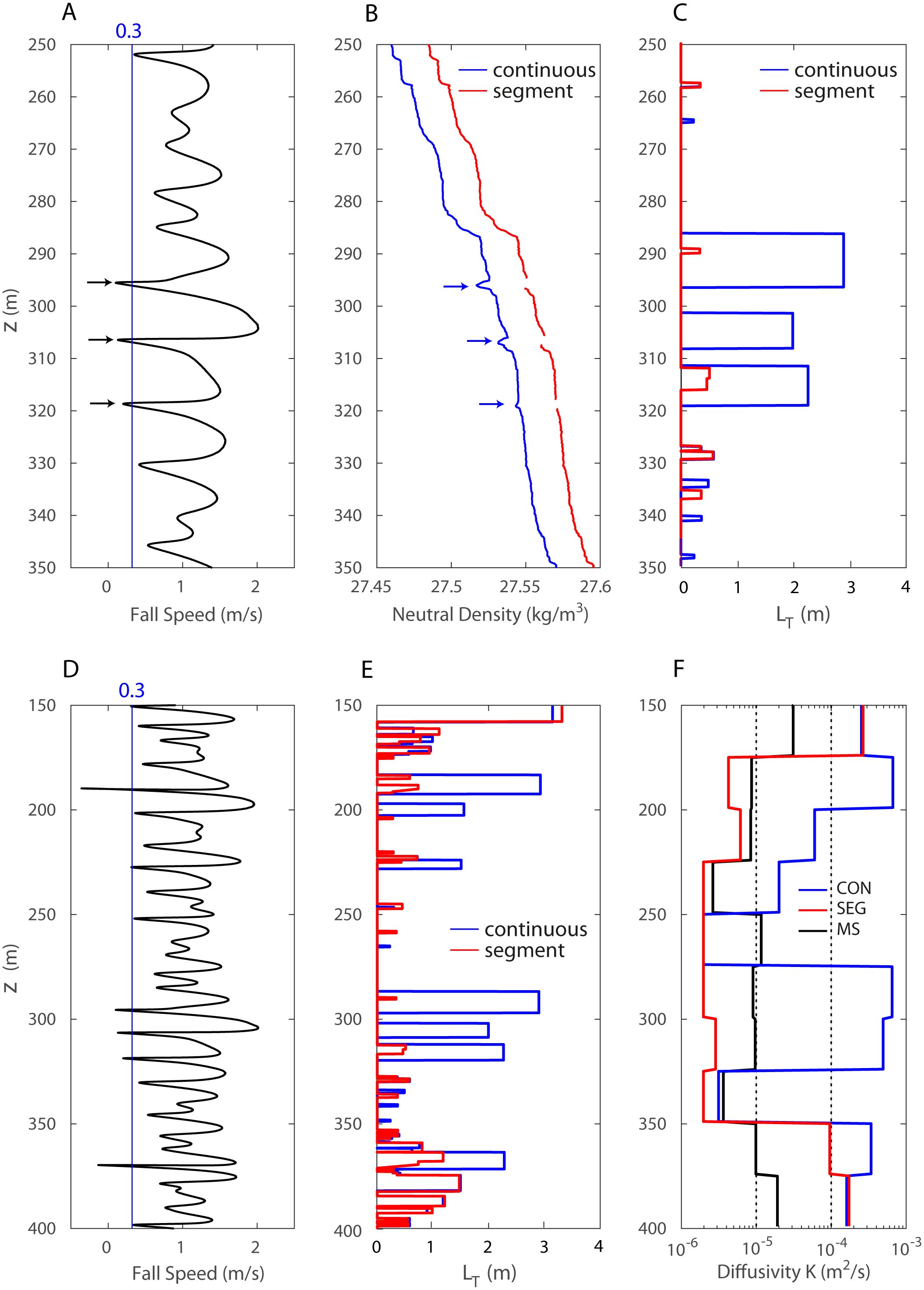
Figure 3. A case study at station A3 (50.7°S, 72°W) occupied during the 2011 KEOPS II cruise in the Kerguelen region (Park et al., 2014). Zoomed profiles in the 250-350-m depth range for (A) CTD fall speed FS, (B) neutral density γ_n, with the segmented profile (red) being offset by 0.03 units, and (C) Thorpe scale L_T. Extended profiles in the 100-400-m depth range for (D) FS, (E) L_T, and (F) diapycnal diffusivity averaged in 25-m bins from continuous (CON, blue) and segment (SEG, red) profiles and microstructure measurements (MS, black). The vertical blue line in (A, D) stands for the threshold value of FS = 0.3 m s^-1. The horizontal arrows in (A, B) indicate the depths where FS < 0.3 m s^-1.

Is there any simple and practical means to circumvent heave-induced false overturns? GG08 suggested for this an overturn ratio R_O criterion, where R_O = min (L⁺/L, L^-/L), L is the total overturn length, and L⁺ (L^-) is the cumulative length occupied by positive (negative) Thorpe displacements. If R_O is less than 0.2, a very skewed ratio likely associated with heave-induced false overturns or spurious spikes, the prospective overturns are considered as being false and rejected on the ground that they might be artificial, as a single perfect overturn sampled straight through the middle would show R_O = 0.5. Park et al. (2014) used a less stringent threshold of R_O = 0.25; we used here the original GG08 criterion (R_O = 0.2) to be consistent with other publications in the literature. We found that many of heave-induced false overturns escape from having been detected by the R_O criterion.

In fact, the abnormal large overturns in the 290-320-m depth range seen in Figure 3C (blue line) are due to heave-induced negative density anomalies in the continuous density profile (see arrows in Figure 3B). Smoothing further the density profiles does not completely remove density inversions. As an alternative approach, we constructed prototype segment profiles (broken red line in Figure 3B), where each segment is disconnected from nearby segments when FS is less than its threshold. As the heave effects disappear a couple of meters below the FS threshold depth, the peak of negative density anomalies shows at the top of each segment, cutting off the density inversion thus removing the heave-induced false overturn. Visual inspection of each zoomed profile has proven necessary to check for any false overturns which could have escaped from the segment-cutting procedure. We found that the FS threshold criterion works very well for the quasi-totality of cases, except for very rare cases where heave-induced false overturns also occurred for FS slightly higher than its threshold in regions of enhanced stratification, such as the case at 200-m depth in Figures 3D, E. Dubious heave-induced false overturns as well as isolated spurious density spikes identified from zoomed visual inspection are removed.

Does it work? In the 290-320-m depth range the segment-by-segment approach (shortly segment approach, hereafter) yields minor overturns with the corresponding L_T varying from zero (solution free) to 0.6 m (Figure 3C, red), which is in stark contrast to much larger L_T of 2-3 m from the conventional continuous profile approach (blue). Outside this heave-affected depth range, there are several narrow bands of minor L_T mostly much less than 1 m, with no significant difference between the two approaches. The entire profile below the surface mixed layer shows that compared to the segment profile (red), the continuous profile (blue) yields a large overestimate of L_T by up to an order of magnitude in regions where FS drops below the threshold, such as at depths around 180, 290, 305, 315 and 370 m (Figure 3E).

K_ρ estimates from the segment approach K_SEG, averaged in 25-m depth bins using the bin-averaged parameters (L_T, N), are shown in Figure 3F, in comparison with those from the concurrent microstructure measurements K_MS (Park et al., 2014) and the conventional Thorpe scale method using the continuous density profile, K_CON. Here we provisionally used the conventional constant L_O/L_T ratio of α = 0.8. A minimum turbulent diffusivity of 2 x 10^-6 m² s^-1 (corresponding to the upper bound of molecular viscosity in the Southern Ocean) is assigned to those bins having no L_T estimates (solution blank regions) or where bin-averaged values are less than 2 x 10^-6 m² s^-1. In the 150-400-m water column K_SEG ranges from 2.0 x 10^-6 m² s^-1 to 2.5 x 10^-4 m² s^-1 with a vertical mean of 2.1 x 10^-5 m² s^-1. These statistics compare reasonably well with those of K_MS ranging from 2.6 x 10^-6 m² s^-1 to 3.1 x 10^-5 m² s^-1 and a vertical mean of 9.2 x 10^-6 m² s^-1. The conventional Thorpe scale method using the continuous profile approach systematically overestimates, with the largest K_CON reaching as much as 8.0 x 10^-4 m² s^-1 and a vertical mean of 9.4 x 10^-5 m² s^-1. The vertical-mean K_CON/K_MS ratio is about 7, although several local maxima larger than 10, with a peak of 80, appear at those depth bins coinciding with large heave-induced false overturns, such as at depths around 190, 290, 310 and 360 m.

2.3 Instrumental density noise and intermediate profiles

It is to be noted that prior to any computation of L_T, intermediate density profiles are previously constructed from treated density profiles, for both continuous and segment profiles. This is because an important constraint in overturn detection is that the density difference between the minima and maxima of a signal must be greater than the noise level of CTD density. GG08 suggested a method originated from Ferron et al. (1998), which only tracks significant differences greater than the threshold density noise level, Δρ, between successive data points. Based on the density data gathered from SBE 9 plus CTDs in the Ross Sea in weak to moderate wind and sea states, GG08 obtained an rms noise level of (1 σ_ρ = 10^-4 kg m^-3) within a well-mixed layer. By setting the threshold level Δρ as the multiple of σ_ρ, GG08 showed that the number of overturns decreases with increasing the multiple and that once the multiple reaches 4-5, further increase makes little change to the number of overturns, to suggest Δρ = 5σ_ρ = 0.0005 kg m^-3. Similarly, Frants et al. (2013) reported that Δρ = 0.0004 kg m^-3 ≡ 4σ_ρ for their SBE 9plus CTDs in the southeastern Pacific and Drake Passage. We tested different numbers of multiple between 3 and 5 to observe that no significant difference in resulting diffusivity estimates with the multiples 3-5, except for decreasing overturns with increasing multiple, as expected. As a practical compromise between the desire to estimate diffusivity at as many vertical points as possible and an acceptable accuracy, we decided to use Δρ = 3σ_ρ = 0.0003 kg m^-3 for constructing the intermediate density profile, with the cost of an 1% risk of taking false overturns as real (assuming the normal distribution of random noise of density). As solution-blank areas increase with increasing Δρ, we suggest that the upper limit in Δρ be 0.0004 kg m^-3. (Too many solution-blank depth bins if Δρ larger than 0.0004 kg m^-3).

2.4 Best-fitting functions between α and L_T

We used four deepest 2010 DIMES CTD stations over the Phoenix Ridge, where concurrent microstructure measurements are available (St. Laurent et al., 2012). The 2010 DIMES survey was carried out during a period of particularly heavy swell, as systematic negative FS (pulling back of the CTD package towards lower pressures) are observed at quasi-regular intervals of 10 m, with a typical swell period of about 10 sec. A selected zoomed profile shows extreme FS values ranging from -0.9 to +2.9 m s^-1, implying that the package oscillation speed w of 1.9 m s^-1 in amplitude was superimposed on the depth-mean FS of about 1.0 m s^-1 (Figure 4A). Assuming a simple sinusoidal swell of ζ = a*sin (ωt), where a is wave amplitude and ω = 2π/T angular frequency with a period of T, the swell-induced vertical package oscillation speed w can be written as: w = dζ/dt = aω*cos (ωt). Using rough estimates for w amplitude (aω = 1.9 m s^-1) and swell period (T = 10 sec), we obtained a = 3.0 m, suggesting that the trough-to-crest swell height (twice a) during the 2010 DIMES survey must have been up to 6 m. The uncertainty of swell period T is estimated at about ±10%, which may yield a swell height uncertainty by the same amount, or ±0.6 m. Effectively, St. Laurent et al. (2012) commented on extreme high seas and winds encountered near the southernmost extent of the Phoenix Ridge. For comparison, in the Kerguelen case FS values are rarely negative (Figure 3D) and the swell height is estimated at about 3 m.

Figure 4

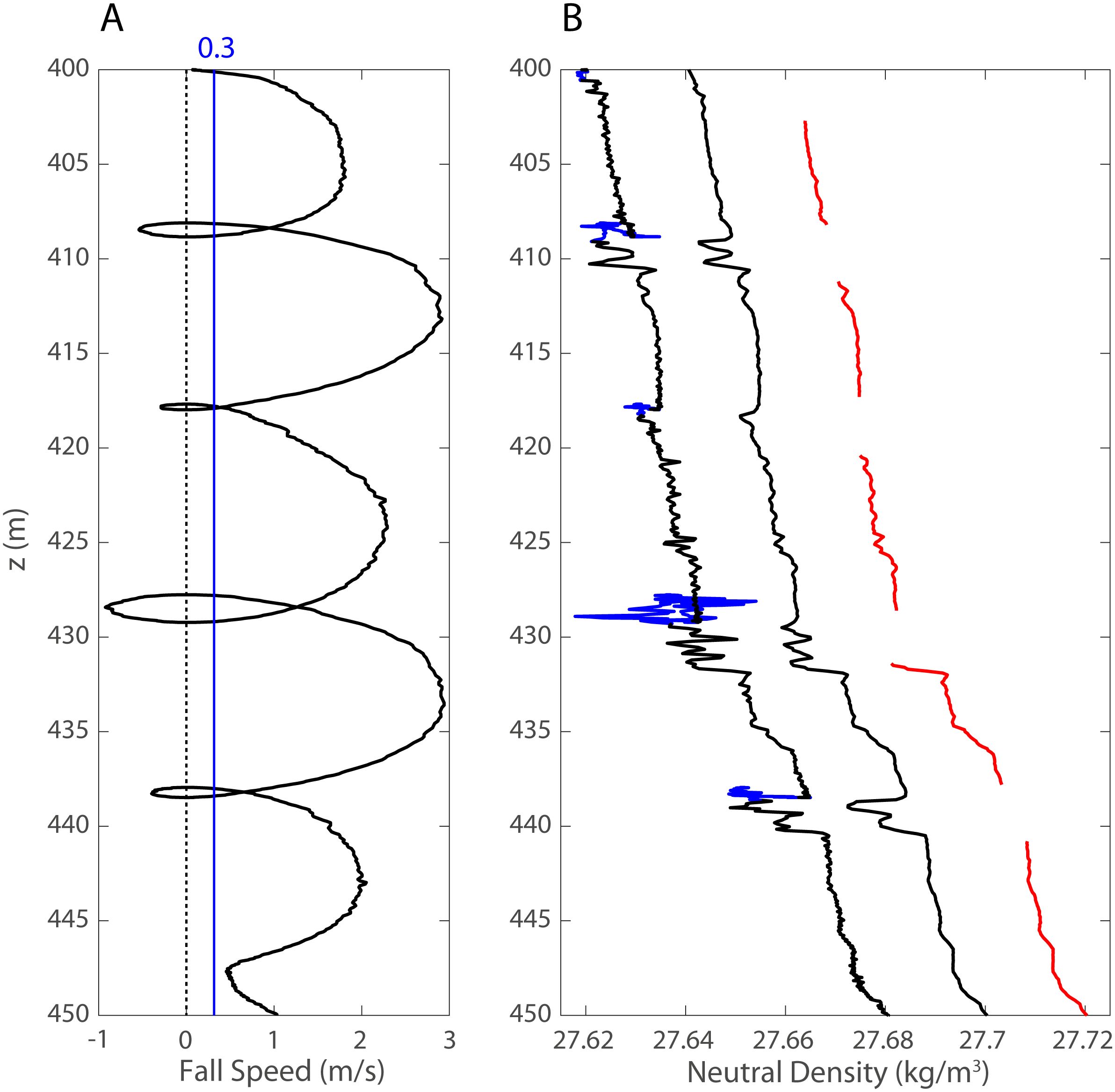
Figure 4. Typical DIMES zoomed profiles of (A) CTD fall speed and (B) density from raw data (left), and processed continuous (middle) and segment (right, red) profiles. In (B) the raw density profiles sampled during package reversals are marked in blue.

In contrast to gradual downward decrease in heave-induced negative density anomalies observed in the Kerguelen case (Figure 3B), the top 2 m of DIMES segment profiles is vigorously perturbed and bears a couple of alternating maxima and minima, suggestive of apparent false overturns (Figure 4B). Residual high-frequency fluctuations, a feature due to imperfect correction of measurement errors (Figure 2), are further intensified in DIMES profiles compared to the Kerguelen case. Therefore, for the particularly disturbed DIMES density profiles collected during a period of heavy swell, we systematically removed the top 2 m of each segment to ensure “cleaned” segment profiles (disconnected red lines in Figure 4B).

Inspired from Mater et al. (2015), who demonstrated a clear tendency of decreasing α with increasing L_T, we checked the statistical relationship between L_O and L_T from DIMES data in the Drake Passage region. L_O values were computed from ε data according to Equation 2, then vertically averaged in 100-m depth bins, similarly to the bin-averaged L_T values estimated from the concurrent CTD density profiles using the segment approach. Consistent with Mater et al. (2015), we observe a decreasing tendency of α with increasing L_T, with the largest α > 1.4 for the smallest L_T < 0.1 m, and much smaller α < 0.8 (mostly around 0.4-0.5 except two outliers) for L_T > 1 m (Figure 5). We overlay in this figure two empirically best-fitting functions between α and L_T, with two negative exponents having different slopes depending on the L_T size relative to 1 m, such as:

Figure 5

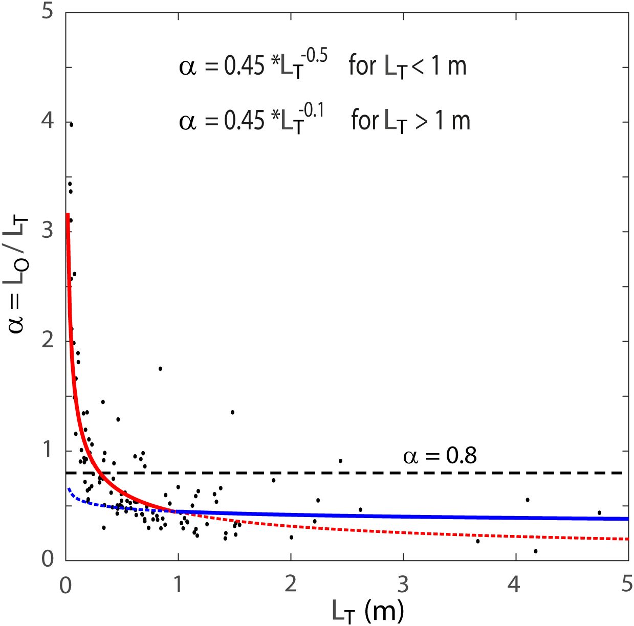
Figure 5. Scatterplot of the Ozmidov to Thorpe scales ratio, α = L_O/L_T, as a function of L_T, calculated from DIMES ε and density profiles over the Phoenix Ridge. The best-fitting α function for L_T greater (less) than 1 m is overlaid by a solid blue (red) curve, in comparison with the constant ratio of α = 0.8 (horizontal dashed line).

$\begin{array}{ll}\alpha =0.45L_T^{-0.5}\text{\hspace{0.17em}\hspace{0.17em}\hspace{0.17em}for\hspace{0.17em}}{L}_T<1\text{m\hspace{0.17em}}(\text{red curve})& (6)\end{array}$

$$\alpha =0.45L_T^{-0.1}\text{\hspace{0.17em}\hspace{0.17em}\hspace{0.17em}for\hspace{0.17em}}{L}_T\ge 1\text{m\hspace{0.17em}}(\text{blue curve})$$

It is clear that the best empirical α functions Equations 6 are completely different from the conventional constant α = 0.8 (horizontal dashed line), with the latter overestimating (underestimating) the former by up to a factor of 2 for L_T greater (less) than 0.3 m. The impact of the α functions on K_ρ is far more serious, climbing up by a factor of 4-5 (see Table 1), as K_ρ is proportional to the square of α according to Equation 5.

3 Diapycnal diffusivities in Drake Passage from the revised Thorpe scale analysis

The revised Thorpe scale analysis was applied to a fine-resolution CTD section occupied during the DRAKE cruise in January 2006 in the westernmost Scotia Sea (Provost et al., 2011; Provost et al., 2022), 100-200 km downstream of the Shackleton Fracture Zone (SFZ) (Figure 6). A detailed description of water masses, fronts, and velocity structures of the section is given in Provost et al. (2011). Analyses of concomitant eddy activity and LADCP transport are given in Barré et al. (2011) and Renault et al. (2011), respectively. The section crossed the five major circumpolar fronts associated with the ACC (Park et al., 2019): the Northern Boundary of ACC (NB) locating over the continental slope off the southeastern tip of South America; the Subantarctic Front (SAF) immediately downstream of an isolated topographic rise with prominent seamounts in the northwestern Yaghan Basin; the Polar Front (PF) near the northern rim of the West Scotia Ridge (WSR); the Southern ACC Front (SACCF) near the southern rim of the WSR before entering into the Ona Basin; the Southern Boundary of ACC (SB) over the continental rise of the South Scotia Ridge (SSR).

Figure 6

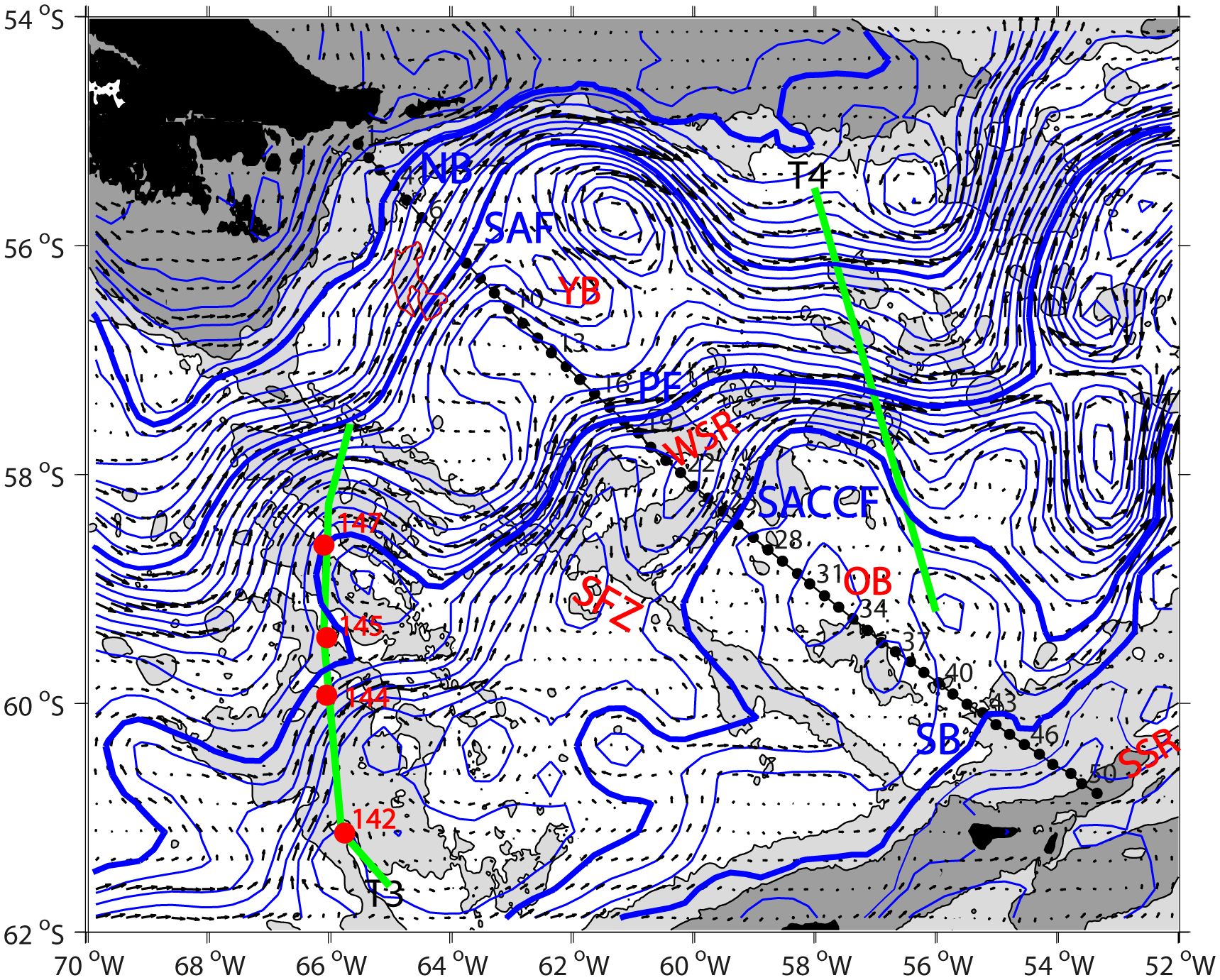
Figure 6. A map showing finely-resolved (~12 nautical miles) CTD/LADCP stations (black dots) occupied during 16-26 January 2006 (Provost et al., 2011). Four red dots over the Phoenix Ridge at 66°W correspond to four deep DIMES CTD stations with concurrent microstructure measurements discussed in subsections 2.4 and 3.1. Two DIMES transects T3 and T4 discussed in Sheen et al. (2013) are shown by green lines. Overlaid are the satellite altimetry-derived dynamic topography averaged over 10 days of the occupation of the 2006 CTD/LADCP stations (blue lines) and the associated surface geostrophic velocity field (arrows). Thick blue lines represent the synoptic dynamic height contours running through the current cores identified in the section by Provost et al. (2011), corresponding to the five major ACC fronts (NB, SAF, PF, SACCF, SB) from Park et al. (2019). Bottom topography with depths shallow than 3500 m (1000 m) is shown lightly (heavily) gray shaded, revealing major topographic features: Shackleton Fracture Zone (SFZ), Yaghan Basin (YB), West Scotia Ridge (WSR), Ona Basin (OB), South Scotia Ridge (SSR). The unnamed prominent seamounts (centered at 64°40’W, 56°20’S) upstream of the DRAKE section in the northwestern Yaghan Basin are indicated by a red contour.

3.1 Comparison of the revised Thorpe scale analysis with DIMES microstructure measurements

In Figure 7 diapycnal diffusivities averaged in 100-m depth bins from the revised Thorpe scale method using the segment approach (K_SEG) are compared with those from the conventional Thorpe scale method using the continuous profile approach and constant α = 0.8 (K_CON), both in reference to the microstructure measurements (K_MS) at the four DIMES stations. K_SEG is further specified into two categories: one using constant α = 0.8 (K_{SEG_α0.8}) and the other using the best-fitting α functions Equations 6 (K_{SEG_Bestα}). Microstructure-derived K_MS (black) shows a general increasing tendency with depth, from a minimum of 4 x 10^-6 m² s^-1 in the upper layer to order 10^-4 m² s^-1 in the abyssal layer, with a peak of 7 x 10^-4 m² s^-1 close to seabed at two occasions (Figure 7A). The conventional Thorpe scale analysis (K_CON, blue) shows an overestimation by up to one to two orders of magnitude at all stations and in most depth bins. Despite very harsh sea states during the 2010 DIMES survey, the segment approach with constant α = 0.8 (K_{SEG_α0.8}, green) yields results significantly improved compared to K_CON, but still showing non-negligible positive biases up to a factor of 10 compared to K_MS. The underestimation tendency seen in the 200-1000-m depth range is due to the frequent occurrence of solution-blank (2 x 10^-6 m² s^-1) depth bins, which is likely related to the excessive smoothing of density profiles in regions of quiet turbulence levels. There also appears a systematic overestimation tendency below 1000-m depth. In contrast, the combined use of the segment approach and best-fitting α functions, K_{SEG_Bestα} (red), yields much better results, removing a large part of positive and negative biases of K_{SEG_α0.8} (green) to agree closely with K_MS (Figure 7A). To be more quantitative, a scatterplot of K_{SEG_α0.8}, K_{SEG_Bestα} and K_CON relative K_MS and the frequency distribution of individual ratios of K_{SEG_α0.8}/K_MS (green), K_{SEG_Bestα}/K_MS (red) and K_CON/K_MS (blue) are shown in Figures 7B, C, respectively. The conventional Thorpe scale analysis shows an overestimation by up to two orders of magnitude, with an ensemble-mean K_CON/K_MS ratio of 9.1. In contrast, the revised Thorpe scale method using both the segment approach and best-fitting α functions provides an ensemble-mean K_{SEG_Bestα}/K_MS ratio of 1.5, with 95% of individual bin ratios lying within a factor of 4, a value comparable to the theoretical uncertainty of 3-4 for an indirect (i.e., shear) method (Polzin et al., 2002). K_{SEG_Bestα} significantly better agrees with K_MS than K_{SEG_α0.8} does, indicating that both the segment approach and best fitting α functions (though less extent) are indispensable for yielding best results.

Figure 7

Figure 7. (A) Profiles of diapycnal diffusivities estimated at four DIMES stations from different approaches: conventional Thorpe scale analysis (K_CON, blue); segment approach with α = 0.8 (K_{SEG_α0.8}, green); segment approach with best-fitting α functions Equations 6 (K_{SEG_Bestα}, red); microstructure measurements (K_MS, black). (B) Scatter plot of K_{SEG_α0.8}, K_{SEG_Bestα} and K_CON relative to K_MS. (C) Frequency distribution (in %) of ratios of K_{SEG_α0.8}, K_{SEG_Bestα} and K_CON relative to K_MS.

3.2 Diapycnal diffusivities from the revised Thorpe scale analysis in the northern Drake Passage

Figure 8 presents the spatial distribution of diapycnal diffusivities along the 2006 DRAKE CTD section from the best-revised Thorpe scale analysis using both the segment approach and best-fitting α functions Equations 6, K_{SEG_Bestα}, which is referred to as K_ρ hereafter, for simplicity. K_ρ estimates averaged in 100-m depth bins range from a default minimum of 2.0 x 10^-6 (solution blank bins) to a maximum of 1.3 x 10^-2 m² s^-1 in the whole section, although the quasi-totality (> 99%) of bins shows a value less than 1 x 10^-3 m² s^-1. This is consistent with DIMES microstructures-derived diffusivities of order 10^-5-10^-3 m² s^-1 in nearby Drake Passage regions (St. Laurent et al., 2012; Sheen et al., 2013).

Figure 8

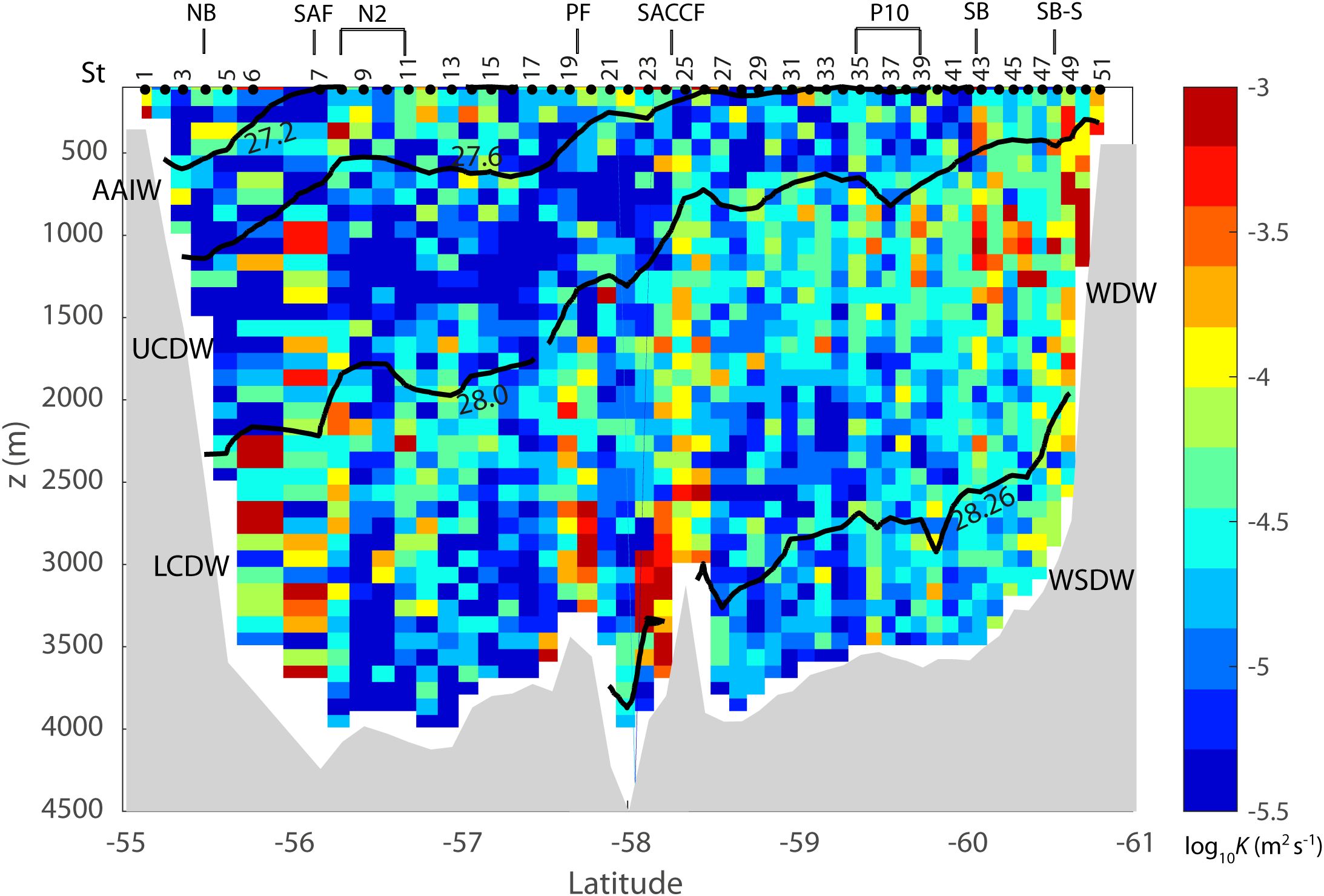
Figure 8. Spatial distribution of K_ρ (in log₁₀ m² s^-1) from revised Thorpe scale analysis along the 2006 DRAKE section. The locations of major frontal branches and eddies (N2, P10) identified by Provost et al. (2011) are indicated by short vertical lines at the top of figure. SB-S stands for an eddy-induced, local southern branch of the SB (see Figure 6). Thick isopycnals (γ_n) mark the boundaries of different water masses.

In the Yaghan Basin enhanced mixing of 10^-4-10^-3 m² s^-1 predominantly occurs in the deep/abyssal layer corresponding to Lower Circumpolar Deep Water (LCDW, 28.0 < γ_n < 28.26 kg m^-3). In the upper layer (γ_n < 27.6 kg m^-3) including Antarctic Intermediate Water (AAIW), the mixing intensity is much weaker and spatially more heterogeneous, although it generally lies between 10^-5 m² s^-1 and 10^-4 m² s^-1. In contrast, the Upper Circumpolar Deep Water (UCDW, 27.6 < γ_n < 28.0 kg m^-3) layer exhibits a middepth mixing minimum of order 10^-5 m² s^-1. The middepth K_ρ estimates of O (10^-5m² s^-1) in the northern Drake Passage are of the same order as those from DIMES microstructure measurements over the Phoenix Ridge at 66°W (transect T3 in Figure 6) (St. Laurent et al., 2012; Sheen et al., 2013). At 57°W (transect T4) where the ACC is most narrowly restricted over rough and shallow topography, Sheen et al. (2013) reported enhanced middepth mixing of O (10^-4 m² s^-1), a value an order of magnitude larger compared to the upstream transect T3 and to the DRAKE section located in midway between T3 and T4.

It is noteworthy that enhanced mixing coincides with the major ACC fronts (SAF, PF, SACCF) except the NB, with mixing intensity increasing towards the bottom up to order 10^-3 m² s^-1 (Figure 8). A similar feature is also observed at the outer rim (56.2°S, 56.7°S) of a cyclonic eddy N2 identified by Provost et al. (2011). In contrast, within inter-frontal zones with weaker flow, just north of the PF at 57.2°S and between the PF and SACCF at 58.0°S, the overall abyssal mixing intensity weakens by a factor of 5 or more. However, the Subantarctic frontal zone between the SAF at station (St.) 7 and the NB at St. 4 features a local mixing maximum of 1.3 x 10^-2 m² s^-1 at 2700-m depth at St. 6. This corresponds to the K_ρ maximum of the whole DRAKE section, which is also associated with a large-scale (~100 m) convective overturn (not shown). While its exact cause deserves a future investigation, such an elevated mixing about 1000 m above the bottom is likely related to an upstream flow-topography interaction as the DRAKE section was located at about 40 km downstream from prominent unnamed seamounts (centered at 64°40’W, 56°20’S and marked in red in Figure 6). Indeed, Nagai et al. (2021) showed that in the Tokara Strait the Kuroshio jet flow over prominent seamounts can generate long-persisting (100 km) downstream streaks of negative (anticyclonic) potential vorticity, trapping near-inertial waves and forming intense mixing hotspots.

3.3 Enhanced middepth mixing due to WDW intrusions in the southern Drake Passage

In contrast to the middepth minimum of O (10^-5 m² s^-1) of UCDW in the northern Drake Passage, a middepth (500-1500 m) mixing maximum of 10^-4-10^-3 m² s^-1 in the southern Ona Basin is centered at the LCDW layer (28.0 < γ_n < 28.26 kg m^-3) and extends locally to the lower half of the UCDW layer (γ_n > 27.8 kg m^-3) (Figure 8). A series of coherent vertical bands of enhanced middepth mixing extend from the continental slope into the interior of the Ona Basin, which is congruent with large intrusions of Warm Deep Water (WDW) as seen by pronounced thermohaline interleaving in the CDW layer (Figure 9A; Provost et al., 2011). WDW is the recently-ventilated cold/fresh variety of LCDW originating from the Weddell-Scotia Confluence developed along the SSR in the northwestern corner of the Weddell Gyre (Naveira Garabato et al., 2002; Whitworth et al., 1994; Patterson and Sievers, 1980). After overflowing through deep passages across the SSR (e.g., Orkney Passage and Phillips Passage to a less extent), WDW and denser Weddell Sea Deep Water (WSDW forming AABW in Drake Passage) flow westward along the continental slope of the SSR before arriving at the southern end of the SFZ (Naveira Garabato et al., 2002). The DRAKE CTD section ran across the southwestern corner of the Scotia Sea (Figure 6), which constitutes the primary source for the ventilation of “old” CDW carried by the ACC and recharge of AABW by inflow of fresher, colder and oxygen-rich Weddell subpolar waters into the southern Drake Passage.

Figure 9

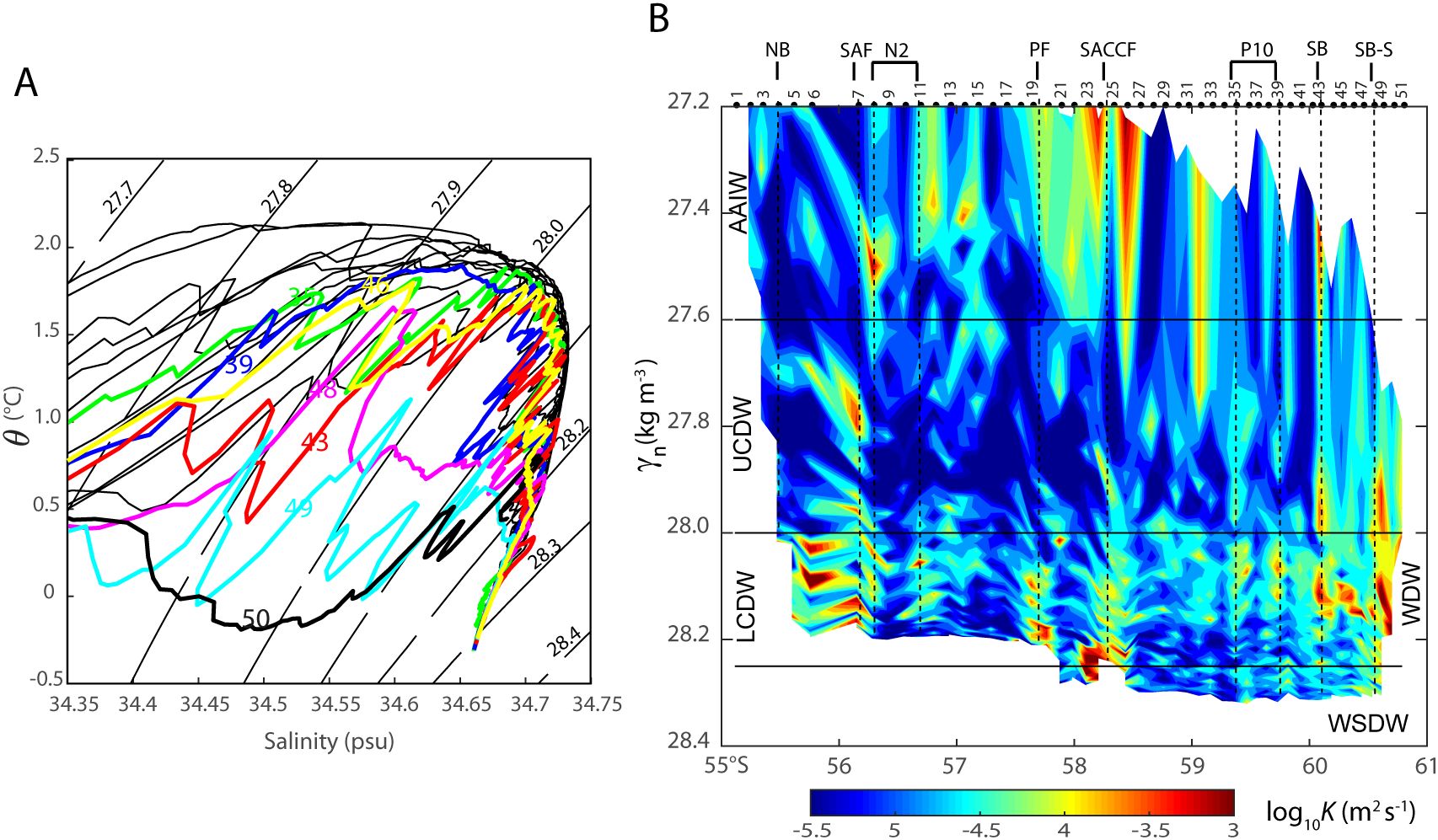
Figure 9. (A) Zoom of the potential temperature-salinity diagram for deep waters in the Ona Basin. Seven stations (35, 39, 43, 46, 48, 49, 50) marked by different colors feature strong interleaving of CDW and WDW. (B) Vertical distribution of K_ρ as a function of neural density for γ_n >27.2 kg m^-3. Note enhanced middepth mixing at the seven stations indicated in (A).

At seven stations (35, 39, 43, 46, 48, 49, 50), we observe a systematic one-to-one correspondence between large WDW intrusions evidenced by pronounced zig-zagged θ-S curves (Figure 9A) and vertically-coherent bands of significantly larger K_ρ than nearby stations (Figure 9B). These stations showing enhanced middepth mixing systematically feature a double diffusive-favorable density ratio (0.5 < R_ρ < 2) (Schmitt, 1979; Ruddick, 1983). Here, R_ρ = Aθ_z/BS_z, A and B are coefficients of thermal expansion and haline contraction, respectively, and θ_z (S_z) is the mean vertical gradient of potential temperature (salinity) computed from smoothed profiles using a 50-m running mean filter, similarly to Merrifield et al. (2016). As a typical example of thermohaline intrusive features, the vertical θ and S profiles and corresponding K_ρand L_T profiles at St. 43 (corresponding to the SB) are shown in Figure 10 (in comparison with St. 42 that is about 22 km apart and without intrusions). St. 43 features colder/fresher, double diffusive-favorable θ/S profiles contrasting with smooth warmer/saltier, double diffusive-unfavorable profiles at St. 42. Compared to St. 42, St. 43 presents pronounced enhancement of mixing by up to an order of magnitude in several depth ranges, such as below 500 m, 700-1400 m, and 2200-2300 m (Figure 10B). These depth ranges coincide with large intrusions of colder/fresher WDW and warmer/saltier LCDW with a dominant vertical scale of 50-200 m, showing a peak K_ρ of 1 x 10^-3 m² s^-1 in the 1100-1200-m depth bin. On the other hand, in the abyssal layer showing least intrusions, weaker K_ρ (~3 x 10^-5 m² s^-1) are comparable at both stations.

Figure 10

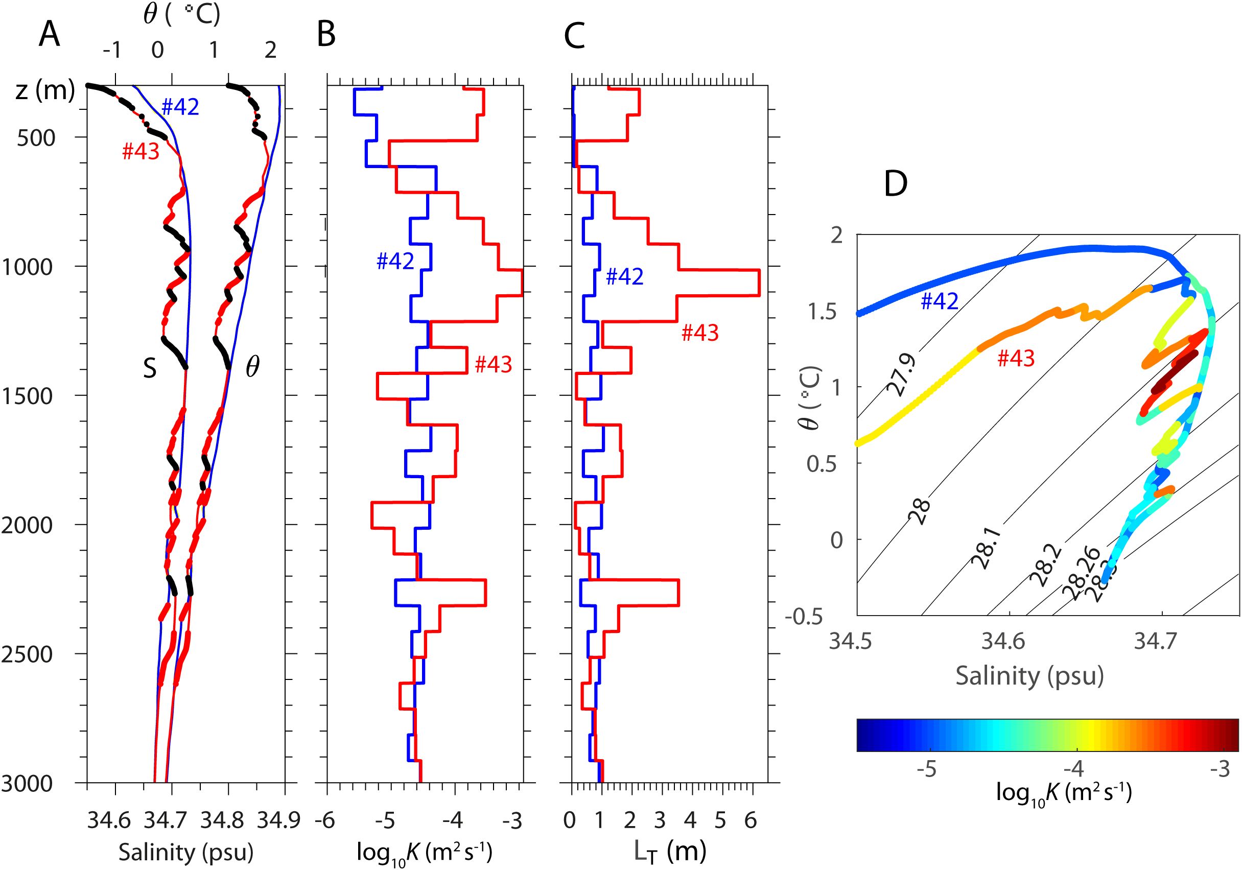
Figure 10. Comparison of two 22 km-apart stations with contrasting profiles of potential temperature (θ), salinity (S), K_ρ, and corresponding L_T. St. 43 features large intrusions and St. 42 has none. (A) θ and S profiles, with thick black (red) segments stand for regions favorable to diffusive convection (salt fingering) with 0.5 < R_ρ < 1 (1 < R_ρ < 2). (B) Comparison of log₁₀ K_ρ profiles at the two stations. (C) Corresponding L_T profiles. (D) θ-S diagrams with superimposed mixing intensities (color). Note that enhanced mixing is systematically found in double-diffusive-favorable intrusive regions at St. 43.

Our results are analogous to those of Merrifield et al. (2016) who highlighted enhanced diapycnal diffusivity in double-diffusive-favorable intrusive regions in the northern Drake Passage, corresponding to the AAIW layer (400-800 m) near the SAF. These authors compared two kinds of diapycnal diffusivities: K_ε from microstructure measurements of ε and based on the Osborn (1980) method; and K_χ from the dissipation rate of thermal variance χ and based on the Osborn and Cox (1972) model. Merrifield et al. (2016) showed that in the double diffusive-favorable intrusive regions K_ε underestimates K_χ by a factor of 3, while they are nearly the same outside those regions. These authors argued that in the double diffusive-favorable intrusive regions χ takes into account of the extra process associated with the intrusion-scale isopycnal eddy flux acting on sharp property gradients generated by lateral stirring.

As the shear method uses the internal wave-driven shear variance to parameterize ε, it is not surprising that the shear method-derived K_ρ by Provost et al. (2011) do not show any evidence for enhanced middepth mixing in the southern Drake Passage. In contrast, the revised Thorpe scale analysis, which is, by construction, free of the constraint of internal wave shear variance, is capable of highlighting the enhanced diapycnal mixing in the WDW intrusive regions in the southwestern Scotia Sea. This indicates at least that the major energy source for enhanced diapycnal mixing here should not be internal waves. Also, despite the existence of a double diffusive-favorable density ratio in the intrusive regions, double diffusive mixing (e.g., salt fingering or diffusive convection) can be safely excluded as it systematically causes downward buoyancy flux, thus it cannot generate observed large density inversions or overturns. The unique potential energy source remained should be enhanced isopycnal eddy stirring as first suggested by Naveira Garabato et al. (2003). We will come back to this point in the discussion section.

Taken together, these results suggest that the tightly-interconnected, enhanced isopycnal eddy stirring and diapycnal mixing processes, commonly congruent with the WDW inflow, are equally important for efficiently ventilating (Provost et al., 2011; Naveira Garabato et al., 2003) and lifting LCDW into the UCDW layer, thus accelerating hand-in-hand the overturning circulation in the southwestern Scotia Sea. This is in line with the Naveira Garabato et al. (2007) paradigm of the “short-circuiting” of overturning circulation in the Scotia Sea arising from the coexistence of eddy-driven isopycnal and diapycnal mixing processes and upwelling of CDW.

4 Discussion

4.1 Revised Thorpe scale method

We presented a revised Thorpe scale method, proposing an innovative segment-by-segment approach for estimating genuine Thorpe scales least affected by heave-induced false overturns. The segment approach consists in performing analysis in each segment independently from adjacent segments separated by the CTD fall speed threshold of 0.3 m s^-1, which is shown to efficiently circumvent false overturns induced by ship heave effects. In addition to the segment approach for minimizing heave effects, which can reduce the overestimation of K_ρ by up to an order of magnitude, we showed that the choice of the Ozmidov to Thorpe scales ratio (α = L_O/L_T) also significantly affects K_ρ estimates. The use of the best-fitting α functions Equations 6 appears indispensable to further reduce, by an extra factor of 4-5, the overestimation when using the conventional constant value of α = 0.8. Consequently, the best-revised Thorpe scale method employing both the segment approach and best-fitting α functions has proven to work very well, yielding most 100-m-bin estimates within a factor of 4 compared to direct microstructure measurements, with an ensemble mean ratio of 1.5 between the two methods (Figure 7). This is an unexpected improvement compared to the conventional Thorpe scale analysis (employing the continuous density profile approach and α = 0.8) that is absolutely inadequate in the swell-prevalent Southern Ocean.

4.2 Middepth mixing maximum in intrusive regions in the southern Drake Passage

The revised Thorpe scale method highlights the most unexpected original feature in the southern Drake Passage corresponding to the southwestern corner of the Scotia Sea. There clearly appears a middepth mixing maximum of 10^-4-10^-3 m² s^-1 in the 500-1500-m depth range corresponding to the LCDW (28.0 < γ_n < 28.26 kg m^-3) layer, locally extending to lower half of the UCDW layer (γ_n > 27.8 kg m^-3) (Figures 8, 9). These unusually-enhanced middepth K_ρ in the southern Drake Passage exceeds the northern Drake Passage counterpart by an order of magnitude. The middepth K_ρ in the southwestern Scotia Sea region is even larger than those in the abyssal layer by a factor of 5, on average. Such unexpected features are systematically congruent with large intrusions of the recently ventilated WDW (a cold/fresh variety of LCDW) originating from the Weddell-Scotia Confluence region, as evidenced by a zig-zagged large θ-S variability along isopycnals (Figure 9A).

Our finding is analogous to the enhanced diapycnal diffusivity in Subantarctic intrusive regions in the northern Drake Passage intermediate water layer (400-800 m), as highlighted by Merrifield et al. (2016). Following these authors and using the density ratio R_ρ criterion, we identified significant double diffusive-favorable intrusive features at a number of stations, which systematically coincide with enhanced middepth K_ρ (Figures 9, 10). Merrifield et al. (2016) concluded that the χ-derived diffusivity from the Osborn and Cox (1972) model is most adequate in intrusive regions for capturing enhanced diapycnal mixing resulting from the isopycnal stirring-eddy interaction.

Why does isopycnal stirring by mesoscale eddies matter for diapycnal mixing? By using a triple decomposition of velocity u and temperature θ into mean (m), mesoscale eddies (e), and microscale turbulence (t) in the temperature variance budget, Ferrari and Polzin (2005) showed that the temperature dissipation rate χ is balanced by the sum of two kinds of temperature variance production, namely mesoscale eddies and turbulence:

$$(u_e{\theta }_e)·\nabla {\theta }_m+(u_t{\theta }_t)·\nabla {\theta }_m=-0.5\chi .$$

The mesoscale eddy contribution (u_eθ_e) · ∇θ_m is dominated by the isopycnal component, (u_eθ_e) · ∇_nθ_m, where ∇_n is parallel to isopycnal surfaces, with a negligible diapycnal component; while the turbulence contribution (u_tθ_t) · ∇θ_m is dominated by the diapycnal component, (u_tθt) · ∇_zθ_m, with a negligible isopycnal component (Ferrari and Polzin, 2005). Therefore, microscale temperature variance (which will be eventually dissipated by molecular diffusivity) can be largely produced by both isopycnal stirring by mesoscale eddies and diapycnal mixing by turbulence.

The large-scale temperature gradient along isopycnals (∇_nθ_m) is maximum in intrusive regions, and enhanced thermohaline interleavings there (Figure 9A) may provide favorable conditions for double-diffusive instabilities. For small R_ρ close to unity, however, shear instabilities coexist due to modulation of wave strain caused by buoyancy flux divergence (Stern et al., 2001). Based on a direct numerical calculation resolving both waves and salt fingering, these authors showed that the temporally increasing wave shear does not reduce the finger fluxes until the wave Richardson number R_i (= N²/S², where S² = u_z² + v_z²) drops to 0.5, whereupon the wave starts to overturn, yielding convective mixing and halting salt fingering. In other words, even in the R_ρ range favorable to both diffusive convection and salt fingering (0.5 < R_ρ < 2), double-diffusive instabilities are feasible for R_i > 0.5 only, while shear instabilities producing large overturns are predominant for R_i < 0.5. Although precise information of R_i is missing, the systematic large overturns (or Thorpe scales) confined in the intrusive regions (Figure 10) suggest that the enhanced mid-depth diapycnal mixing of southern Drake Passage should result from shear instabilities, as double-diffusive instabilities themselves do not yield any overturns. This is in stark contrast to the northern Drake Passage intrusive regions, where diapycnal mixing owes largely to double-diffusive instabilities, as concluded by Merrifield et al. (2016). These authors showed that ε-derived K_ρ there is inadequate for diapycnal mixing caused by double-diffusive instabilities, which is not the case of the southern Drake Passage intrusive regions, as shear instabilities constitute a primary agency for diapycnal mixing in the latter regions.

4.3 Climatic implications for the meridional overturning circulation in the Southern Ocean

Finally, we would like to comment that the middepth mixing maximum in the southern Drake Passage highlighted by the revised Thorpe scale analysis has important climatic implications for the meridional overturning circulation in the Southern Ocean. Based on the analysis of seven climate models, Chen et al. (2023) investigated the impacts of a warming climate-induced Antarctic meltwater on decreased open-ocean deep convection, deep-ocean warming and AABW volume contraction, suggesting that these features could be associated with the southward shift of CDW and the weakening of the lower overturning cell. In effect, the southern Scotia Sea region comprises the clockwise (relative to the eastward flowing ACC) lower overturning cell across the ACC (Figure 11). Based on an idealized numerical model, Ito and Marshall (2008) showed that the strength of the lower overturning cell is strongly controlled by the magnitude of abyssal diapycnal mixing and isopycnal stirring. Previous idealized model studies (e.g., Ito and Marshall, 2008; Mashayek et al., 2015) considered varying degrees and shapes of enhanced abyssal mixing. It may be instructive to test how the results change if a middepth mixing maximum (mimicking our inference in the southern Drake Passage) were rather inserted in their models. We expect an outstanding middepth branch showing enhanced diapycnal mixing and upwelling in the LCDW layer, which extends into the UCDW layer (see Figure 9B), thereby strengthening the upper overturning cell. Such a short-circuiting of the meridional overturning circulation (from the lower cell to the upper cell) should occur despite the overall weakening of the lower overturning cell due to AABW volume contraction in a warming climate (Chen et al., 2023). This interpretation is consistent with the recent tendency of weakening (strengthening) lower (upper) overturning cell in the Southern Ocean due to human-induced climate change (Lee et al., 2023). To test empirically our inference, dedicated field surveys of microstructure measurements of shear ε and thermal variance χ in the poorly sampled but climatically-critical southwestern Scotia Sea region are needed.

Figure 11

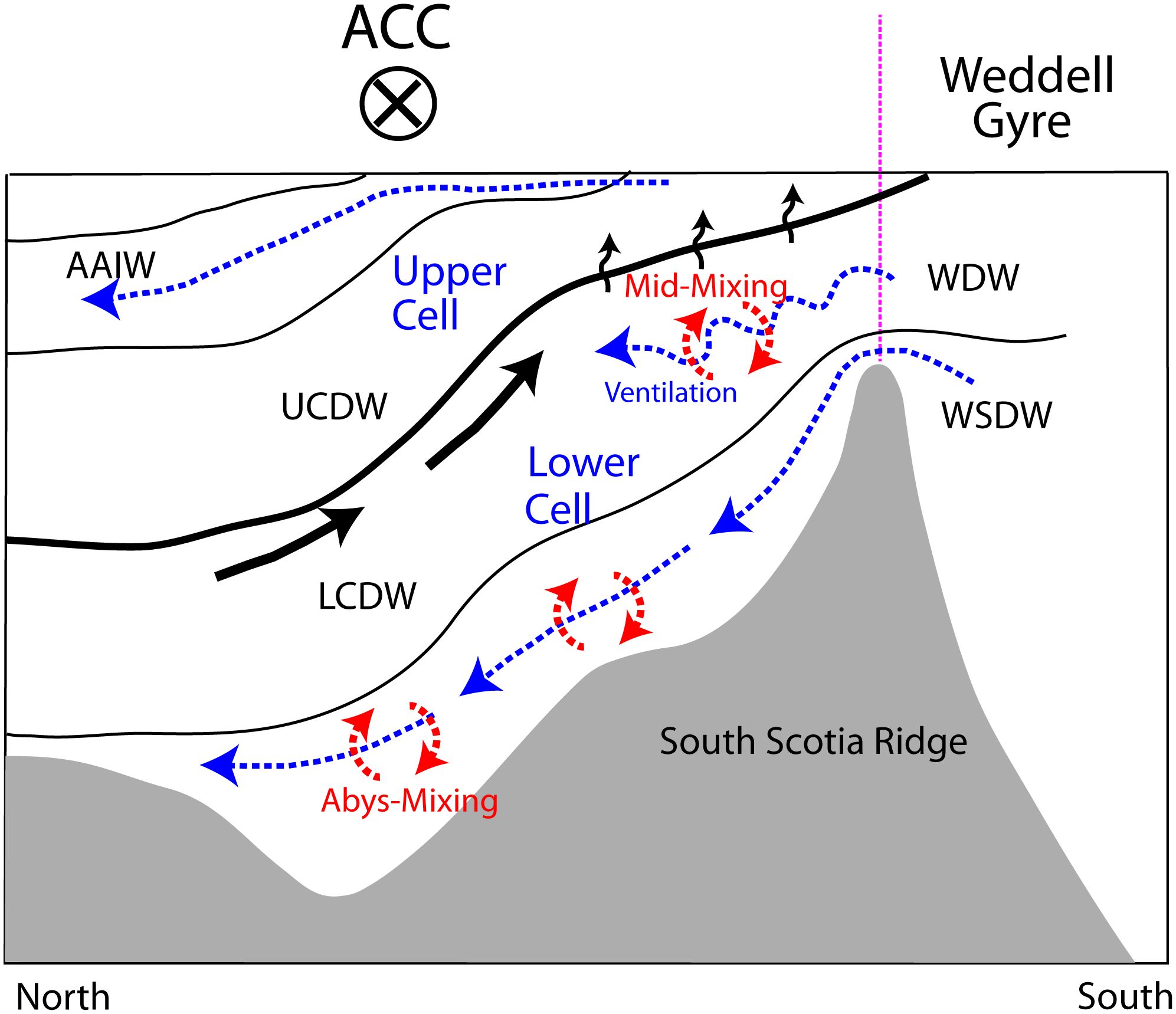
Figure 11. Schematic of the meridional overturning circulation across the ACC in the western Scotia Sea region, as diagnosed by the present study. Strengthened overturning circulation in the lower cell is expected due to WDW intrusions, enhancing middepth diapycnal mixing (mid-mixing), isopycnal stirring (ventilation) and upwelling of LCDW (wavy arrows), in addition to abyssal mixing (abys-mixing) of inflowing WSDW. Inspired from diagrams of Naveira Garabato et al. (2003) and Ito and Marshall (2008).

Data availability statement

The datasets presented in this study can be found in online repositories. The names of the repository/repositories and accession number(s) can be found in the article/supplementary material.

Author contributions

YP: Conceptualization, Investigation, Methodology, Supervision, Writing – original draft, Writing – review & editing. ID: Formal analysis, Software, Validation, Visualization, Writing – review & editing. JL: Data curation, Writing – review & editing. CP: Data curation, Funding acquisition, Writing – review & editing.

Funding

The author(s) declare financial support was received for the research, authorship, and/or publication of this article. This study is a contribution to the CNES-funded BACI project. J-HL is supported by the ‘UN Ocean Decade Implementation Research Group Project (RS-2023-00256732)’ financed by the Ministry of Oceans and Fisheries of Korea.

Acknowledgments

Raw CTD data gathered along the Phoenix Ridge during the 2010 DIMES survey have been kindly tracked and communicated by John Toole from Woods Hole Oceanographic Institution. We are grateful to CNES (Centre National d’Etudes Spatiales) for constant support.

Conflict of interest

Author J-HL was employed by GeoSystem Research Corporation. The remaining authors declare that the research was conducted in the absence of any commercial or financial relationships that could be construed as a potential conflict of interest.

Publisher’s note

All claims expressed in this article are solely those of the authors and do not necessarily represent those of their affiliated organizations, or those of the publisher, the editors and the reviewers. Any product that may be evaluated in this article, or claim that may be made by its manufacturer, is not guaranteed or endorsed by the publisher.

References

Barré N., Provost C., Renault A., Sennéchael N. (2011). Fronts, meanders and eddies in Drake Passage during the ANT-XXIII/3 cruise in January-February 2006: a satellite perspective. Deep-Sea Res. II 58, 2533–2554. doi: 10.1016/j.dsr2.2011.01.003

Crossref Full Text | Google Scholar

Chen J.-J., Swart N. C., Beadling R., Cheng X., Hattermann T., Juling A., et al. (2023). Reduced deep convection and bottom water formation due to Antarctic meltwater in a multi-model ensemble. Geophys. Res. Lett. 50, e2023GL106492. doi: 10.1029/2023GL106492

Crossref Full Text | Google Scholar

Dillon T. M. (1982). Vertical overturns: A comparison of Thorpe and Ozmidov length scales. J. Geophys. Res. 87, 9601–9613. doi: 10.1029/jc087ic12p09601

Crossref Full Text | Google Scholar

Ferrari R., Polzin K. L. (2005). Finescale structure of the T–S relation in the eastern North Atlantic. J. Phys. Oceanogr. 35, 1437–1454. doi: 10.1175/JPO2763.1

Crossref Full Text | Google Scholar

Ferron B., Mercier H., Speer K., Gargett A., Polzin K. (1998). Mixing in the romanche fracture zone. J. Phys. Oceanogr. 28, 1929–1945. doi: 10.1175/1520-0485(1998)028<1929:MITRFZ>2.0.CO;2

Crossref Full Text | Google Scholar

Frants M., Damerell G. M., Gille S. T., Heywood K. J., MacKinnon J., Sprintall J. (2013). An assessment of density based fine-scale methods for estimating diapycnal diffusivity in the Southern Ocean. J. Atmos. Ocean. Tech. 30, 2647–2661. doi: 10.1175/JTECH-D-12-00241.1

Crossref Full Text | Google Scholar

Galbraith P. S., Kelley D. E. (1996). Identifying overturns in CTD profiles. J. Atmos. Ocean. Tech. 13, 688–702. doi: 10.1175/15200426(1996)013<0688:IOICP>2.0.CO;2

Crossref Full Text | Google Scholar

Gargett A., Garner T. (2008). Determining Thorpe scales from ship lowered CTD density profiles. J. Atmos. Ocean. Tech. 25, 1657–1670. doi: 10.1175/2008JTECHO541.1

Crossref Full Text | Google Scholar

Gregg M. C., Kunze E. (1991). Shear and strain in Santa Monica basin. J. Geophys. Res. 96, 16 709–16 719. doi: 10.1029/91JC01385

Crossref Full Text | Google Scholar

He Y., Zhu X., Sheng Z., He M. (2024). Identification of stratospheric disturbance information in China based on the round-trip intelligent sounding system. Atm. Chem. Phys. 24, 3839–3856. doi: 10.5194/acp-24-3839-2024

Crossref Full Text | Google Scholar

Ito T., Marshall J. (2008). Control of lower-limb overturning circulation in the Southern Ocean by diapycnal mixing and mesoscale eddy transfer. J. Phys. Oceanogr. 38, 2832–2845. doi: 10.1175/2008JPO3878.1

Crossref Full Text | Google Scholar

Ko H. C., Chun H. Y. (2022). Potential sources of atmospheric turbulence estimated using the Thorpe method and operational radiosonde data in the United States. Atmos. Res. 265, 105891. doi: 10.1016/j.atmosres.2021.105891

Crossref Full Text | Google Scholar

Kunze E., Firing E., Hummon J., Chereskin T., Thurnherr A. M. (2006). Global abyssal mixing inferred from lowered ADCP shear and CTD strain profiles. J. Phys. Oceanogr. 36, 1553–1576. doi: 10.1175/JPO2926.1

Crossref Full Text | Google Scholar

Kunze E., Kennelly A., Sanford T. B. (1992). The depth dependence of shear fine structure off Point Arena and near Pioneer Seamount. J. Phys. Oceanogr. 22, 29–41. doi: 10.1175/1520-0485-22.1.29

Crossref Full Text | Google Scholar

Ledwell J. R., St. Laurent L. C., Girton J. B., Toole J. M. (2011). Diapycnal mixing in the antarctic circumpolar current. J. Phys. Oceanogr. 41, 241–246. doi: 10.1175/2010JPO4557.1

Crossref Full Text | Google Scholar

Lee S.-K., Lumpkin R., Gomez F., Yeager S., Lopez H., Takglis F., et al. (2023). Human-induced changes in the global meridional overturning circulation are emerging from the Southern Ocean. Commun. Earth Environ. 4, 1–12. doi: 10.1038/s43247-023-00727-3

Crossref Full Text | Google Scholar

Mashayek A., Ferrari R., Nikurashin M., Peltier W. R. (2015). Influence of enhanced diapycnal mixing on stratification and the ocean overturning circulation. J. Phys. Oceanogr. 45, 2580–2597. doi: 10.1175/JPO-D-15-0039.1

Crossref Full Text | Google Scholar

Mater B. D., Venayagamoorthy S. K., St. Laurent L., Moum J. N. (2015). Biases in Thorpe-scale estimates of turbulence dissipation. Part I: Assessments from large-scale overturns in oceanographic data. J. Phys. Oceanogr. 45, 2497–2521. doi: 10.1175/JPO-D-14-0128.1

Crossref Full Text | Google Scholar

Merrifield S. T., St. Laurent L., Owens B., Thurnherr A. M., Toole J. M. (2016). Enhanced diapycnal diffusivity in intrusive regions of the Drake Passage. J. Phys. Oceanogr. 46, 1309–1321. doi: 10.1175/JPO-D-15-0068.1

Crossref Full Text | Google Scholar

Munk W. (1966). Abyssal recipes. Deep-Sea Res. 13, 707–730. doi: 10.1016/0011-7471(66)90602-4

Crossref Full Text | Google Scholar

Nagai T., Hasegawa D., Tsutsumi E., Nakamura H., Nishina A., Senjyu T., et al. (2021). The Kuroshio flowing over seamounts and associated submesoscale flows drive 100-km-wide 100-1000-hold enhancement of turbulence. Commun. Earth Environ. 2, 1–11. doi: 10.1038/s43247-021-00230-7

Crossref Full Text | Google Scholar

Naveira Garabato A. C., Heywood K. J., Stevens D. P. (2002). Modification and pathways of Southern Ocean deep waters in the Scotia Sea. Deep-Sea Res. I 49, 681–705. doi: 10.1016/S0967-0637(01)00071-1

Crossref Full Text | Google Scholar

Naveira Garabato A. C., Polzin K., King B., Heywood K. J., Visbeck M. (2004). Widespread intense turbulent mixing in the Southern Ocean. Science 303, 210–213. doi: 10.1126/science.1090929

PubMed Abstract | Crossref Full Text | Google Scholar

Naveira Garabato A. C., Stevens D. P., Heywood K. J. (2003). Water mass conversion, fluxes, and mixing in the Scotia Sea diagnosed by an inverse model. J. Phys. Oceanogr. 33, 2565–2587. doi: 10.1175/1520-0485(2003)033<2565:WMCFAM>2.0.CO;2

Crossref Full Text | Google Scholar

Naveira Garabato A. C., Stevens D. P., Watson A. J., Roether W. (2007). Short-circuiting of the overturning circulation in the Antarctic Circumpolar Current. Nat. Lett.447, 194–197. doi: 10.1038/nature05832

Crossref Full Text | Google Scholar

Osborn T. R. (1980). Estimates of the local rate of vertical diffusion from dissipation measurements. J. Phys. Oceanogr. 10, 83–89. doi: 10.1175/1520-0485(1980)010<0083:EOTLRO>2.0.CO;2

Crossref Full Text | Google Scholar

Osborn T. R., Cox C. S. (1972). Oceanic fine structure. Geophy. Fluid. Dyn. 3, 321–345. doi: 10.1080/03091927208236085

Crossref Full Text | Google Scholar

Ozmidov R. V. (1965). On the turbulent exchange in a stably stratified ocean. Izu. Acad. Sci. USSR Atmos. Ocean. Phys. (Engl. Trans.) 8, 853–860.

Google Scholar

Park Y.-H., Durand I., Lee J.-H., Provost C. (2022). Raw CTD data and microstructure measurements for revisiting Thorpe scale analysis of diapycnal mixing in the Southern Ocean. doi: 10.17882/89861

PubMed Abstract | Crossref Full Text | Google Scholar

Park Y.-H., Lee J.-H., Durand I., Hong C.-S. (2014). Validation of Thorpe-scale-derived vertical diffusivities against microstructure measurements in the Kerguelen region. Biogeosciences 11, 6927–6937. doi: 10.5194/bg-11-6927-2014

Crossref Full Text | Google Scholar

Park Y.-H., Park T., Kim T.-W., Lee S.-H., Hong C.-S., Lee J.-H., et al. (2019). Observations of the Antarctic Circumpolar Current over the Udintsev Fracture Zone, the narrowest choke point in the Southern Ocean. J. Geophys. Res. Ocean 124, 4511–4528. doi: 10.1029/2019JC015024

Crossref Full Text | Google Scholar

Patterson S. L., Sievers H. A. (1980). The weddell-scotia confluence. J. Phys. Oceanogr. 10, 1584–1610. doi: 10.1175/1520-0485(1980)010<1584:TWSC>2.0.CO;2

Crossref Full Text | Google Scholar

Polzin K. L., Kunze E., Hummon J., Firing E. (2002). The finescale response of lowered ADCP velocity profiles. J. Atmos. Ocean. Tech. 19, 205–224. doi: 10.1175/1520-0426(2002)019<0205:TFROLA>2.0.CO;2

Crossref Full Text | Google Scholar

Provost C., Renault A., Barré N., Sennéchael N., Garçon V., Sudre J., et al. (2011). Two repeat crossings of Drake Passage in austral summer 2006: Short-term variations and evidence for considerable ventilation of intermediate and deep waters. Deep-Sea Res. II 58, 2555–2257. doi: 10.1016/j.dsr2.2011.06.009

Crossref Full Text | Google Scholar

Provost C., Sennéchael N., Park Y.-H., Durand I. (2022). Hydrographic data from the south-bound Drake 2006 section. doi: 10.17882/89642

Crossref Full Text | Google Scholar

Renault A., Provost C., Sennéchael N., Barré N., Kartavtseff A. (2011). Two full-depth velocity sections in the Drake Passage in 2006-Transport estimates. Deep-Sea Res. II 58, 2572–2591. doi: 10.1016/j.dsr2.2011.01.004

Crossref Full Text | Google Scholar

Ruddick B. R. (1983). A practical indicator of the stability of the water column to double-diffusive activity. Deep-Sea Res. 30, 1105–1107. doi: 10.1016/0198-0149(83)90063-8

Crossref Full Text | Google Scholar

Schmitt R. W. (1979). The growth rate of super-critical salt fingers. Deep-Sea Res. 26A, 23–40. doi: 10.1016/0198-0149(79)90083-9

Crossref Full Text | Google Scholar

Sheen K. L., Brearley J. A., Naveira Garabato A. C., Smeed D. A., Waterman S., Ledwell J. R., et al. (2013). Rates and mechanisms of turbulent dissipation and mixing in the Southern Ocean: Results from the Diapycnal and Isopycnal Mixing Experiment in the Southern Ocean (DIMES). J. Geophys. Res. Ocean 118, 2774–2792. doi: 10.1002/jgrc.20217

Crossref Full Text | Google Scholar

Sloyan B. M. (2005). Spatial variability of mixing in the Southern Ocean. Geophys. Res. Lett. 32, L18603. doi: 10.1029/2005GL023568

Crossref Full Text | Google Scholar

Stern M. E., Radko T., Simeonov J. (2001). Salt fingers in an unbounded thermocline. J. Mar. Res. 59, 355–390. doi: 10.1357/002224001762842244

Crossref Full Text | Google Scholar

St. Laurent L. C., Naveira Garabato A. C., Ledwell J. R., Thurnherr A. M., Toole J. M., Watson A. J. (2012). Turbulence and diapycnal mixing in Drake Passage. J. Phys. Oceanogr. 42, 2143–2152. doi: 10.1175/JPO-D-12-027.1

Crossref Full Text | Google Scholar

Thompson A. F., Gille S. T., MacKinnon J. A., Sprintall J. (2007). Spatial and temporal patterns of small-scale mixing in Drake Passage. J. Phys. Oceanogr. 37, 572–592. doi: 10.1175/JPO3021.1

Crossref Full Text | Google Scholar

Thorpe S. A. (1977). Turbulence and mixing in a Scottish loch. Phil. Trans. R. Soc 286A, 125–181. doi: 10.1098/rsta.1977.0112

Crossref Full Text | Google Scholar

Toole J. M., Doherty K. W., Frye D. E., Millard R. C. (1997). A wire guided, free-fall system to facilitate shipborne hydrographic profiling. J. Atmos. Ocean. Tech. 14, 667–675. doi: 10.1175/1520-0426(1997)014<0667:AWGFFS>2.0.CO;2

Crossref Full Text | Google Scholar

Waterhouse A. F., MacKinnon J. A., Nash J. D., Alford M. H., Kunze E., Simmons H. L., et al. (2014). Global pattern of diapycnal mixing from measurements of the turbulent dissipation rate. J. Phys. Oceanogr. 44, 1854–1872. doi: 10.1175/JPO-D-13-0104.1

Crossref Full Text | Google Scholar

Waterman S., Naveira Garabato A. C., Polzin K. L. (2013). Internal waves and turbulence in the Antarctic Circumpolar Current. J. Phys. Oceanogr. 43, 259–282. doi: 10.1175/JPO-D-11-0194.1

Crossref Full Text | Google Scholar

Waterman S., Polzin K. L., Naveira Garabato A. C., Sheen K. L., Forryan A. (2014). Suppression of internal wave breaking in the Antarctic Circumpolar Current near topography. J. Phys. Oceanogr. 44, 1466–1492. doi: 10.1175/JPO-D-12-0154.1

Crossref Full Text | Google Scholar

Whitworth I. I. I. T., Nowlin Jr. W.D., Orsi A. H., Locarnini R. A., Smith S. G. (1994). Weddell Sea shelf water in the Bransfield Strait and Weddell–Scotia Confluence. Deep-Sea Res. 41A, 629–641. doi: 10.1016/0967-0637(94)90046-9

Crossref Full Text | Google Scholar