GWSM4C-NS: improving the performance of GWSM4C in nearshore sea areas

Predicting nearshore significant wave heights (SWHs) with high accuracy is of great importance for coastal engineering activities, marine and coastal resource studies, and related operations. In recent years, the prediction of SWHs in two-dimensional fields based on deep learning has been gradually emerging. However, predictions for nearshore areas still suffer from insufficient resolution and poor accuracy. This paper develops a NS (NearShore) model based on the GWSM4C model (Global Wave Surrogate Model for Climate simulations). In the training area, the GWSM4C -NS model achieved a correlation coefficient (CC) of 0.977, with a spatial Root Mean Square Error (RMSE), annual mean spatial relative error (MAPE), and annual mean spatial absolute error (MAE) of 0.128 m, 10.7%, and 0.103 m, respectively. Compared to the GWSM4C model’s predictions, the RMSE and MAE decreased by 59% and 60% respectively, demonstrating the model’s effectiveness in enhancing nearshore SWH predictions. Additionally, applying this model to untrained sea areas to further validate its learning capability in wave energy propagation resulted in a CC of 0.951, with RMSE, MAPE, and MAE of 0.161m, 12.9%, and 0.137m, respectively. The RMSE and MAE were 43% and 39% lower than the GWSM4C model’s interpolated predictions. The results shown above suggest that the newly proposed model can effectively improve the performance of GWSM4C in nearshore areas.

1 Introduction

Nearshore waves are among the most critical dynamic factors in the coastal marine environment, posing threats to the safety and stability of coastal structures, causing coastal sediment movement, coastal changes, and nearshore water exchanges (Song et al., 2009). The accurate calculation of nearshore waves can effectively prevent marine disasters (Mahjoobi and Mosabbeb, 2009), guide aquaculture (Waseda et al., 2012), and ensure the safety of vessel navigation (Waseda et al., 2014), among other benefits. Significant wave height (SWH) is an indispensable parameter for assessing wave energy and critical meteorological conditions in marine activities. Traditional methods solve the spectral balance equation, including source and sink terms, to obtain SWH. Currently, the most mature models are third-generation wave models, such as SWAN, Wave Watch III, and MASNUM-WAM (Yuan et al., 1991, 1992). Traditional numerical prediction methods have the advantages of physical simulation and data-driven capabilities (Wei et al., 2013); however, they consume significant computational resources and time, making timely predictions difficult in emergencies and limiting the ability to predict wave developments quickly and accurately.

In recent years, rapid advancements in machine learning have provided technical support for addressing complex physical mechanisms, leveraging its strong nonlinear capabilities. Numerous researchers have applied machine learning techniques to the task of predicting SWH, noting their ability to make rapid predictions without requiring extensive computational resources. The application of machine learning in wave height prediction is becoming increasingly widespread, but most applications have been limited to single-point predictions (Makarynskyy, 2004; Londhe, 2008; Jin et al., 2019; Fan et al., 2020; Hu et al., 2021). In practical applications, it is often necessary to understand the wave conditions within a region. Zhou et al. (2021) used the ConvLSTM model, inputting historical SWH data to achieve short-term predictions of SWHs in China’s nearshore areas. Han et al. (2022) and Kim et al. (2022) improved the accuracy of SWH predictions by using historical wind fields and historical wave field elements as inputs to ConvLSTM. Qu et al. (2022) achieved ocean-scale wave element forecasts with accuracy comparable to numerical forecasts. Cao et al. (2023) improved the spatiotemporal prediction algorithm based on the Recurrent Neural Network (PredRNN) by integrating wind and wave elements from both historical and future time steps as model inputs. This enhancement aims at predicting SWH, thereby improving the forecast accuracy for extended periods ranging from 12 hours to 72 hours.

From the above literature, it can be seen that two-dimensional field SWH predictions often use historical wind fields and wave-related elements as inputs, using ConvLSTM and PredRNN as the base model to extract temporal and spatial features of waves and achieve SWH predictions (Shi et al., 2015; Wang et al., 2022). This can achieve good prediction results over moment; however, the process of automatic feature extraction by the model does not correspond to the respective processes of wave generation, propagation, and dissipation. Additionally, the time-series-based approaches used in wave simulations still rely heavily on the given initial wave states, which can result in cumulative errors beyond control with increasing iterations. Recently, the GWSM4C (Global Wave Surrogate Model for Climate simulation) model has been proposed (Jin et al., 2024), it is an economical and feasible wave model. GWSM4C overcomes such limitation by generating initial condition for each prediction moment simultaneously as the simulation is going on. Therefore, cumulative errors due to a fix initial state can be avoided. The current version of GWSM4C focuses on the global ocean, only land and sea points can be identified, and the refraction effects of water depth on wave propagation in nearshore areas are ignored.

Furthermore, since nearshore areas require higher resolution and accuracy in practical applications, the GWSM4C is not good enough results for nearshore regions. To predict SWHs with high spatial resolution and improve the accuracy of GWSM4C in nearshore areas, this study establishes a NS (NearShore) model based on GWSM4C with the consideration of physical mechanisms of wave propagation and depth variation in intermedia waters.

The remainder of this paper is structured as follows: The “Materials and Methods” section introduces the data we used, and describes the theoretical methods and model construction, as well as evaluation metrics. The “Results” section presents the model’s prediction results and analyzes the model’s effectiveness from multiple perspectives. Finally, our “Discussion” section primarily discusses the model’s generalization capability in non-training areas and proposes future research suggestions.

The remainder of this paper is organized as follows. In Section 2, the dataset, model structure, evaluation metrics, and details regarding the training and testing of the GWSM4C-NS are presented. Section 3 provides a comprehensive evaluation and analysis of the prediction ability of GWSM4C-NS, and Section 4 discusses certain key characteristics of GWSM4C-NS. Finally, the conclusions are presented in Section 5.

2 Materials and methods

2.1 Data and preprocessing

The Data adopted in this study is listed in Table 1. As shown in this table, wind field data are sourced from the ECMWF’s ERA-5 dataset (the fifth generation European Centre for Medium-Range Weather Forecasts atmospheric reanalysis of the global climate), with a spatial resolution of 1/4°. The topographic data come from the ETOPO1 global relief model published by the US National Geophysical Data Center. The initial wave field (IWF) are generated using the GWSM4C with a spatial resolution of 1/2°. The SWH data of the target (TAR) are obtained through simulations using the MASNUM-WAM, employing the aforementioned wind and topographic data as inputs, simulating a SWH within the geographic extent of 90°E to 150°E and from 10°S to 50°N, with a spatial resolution of 1/32°. It is important to note that this range is broader than the study area defined in this paper, ensuring that the simulated SWH data contain ample information about the swells. The study area is defined as a portion of nearshore areas of the East China Sea and the South China Sea (areas with water depth less than or equal to 200m are considered nearshore), including the coastal areas from 116°E to 126°E and from 19°N to 29°N. The study periods are the years 2018 and 2020. Data time resolution is one hour.

Table 1

Table 1 The introduction of the data.

To improve the quality of the training dataset, the data underwent several preprocessing steps, including interpolation, masking, normalization, and dataset division. The specific procedures are as follows: Initially, the data resolution was standardized by linearly interpolating wind field data, bathymetry, and IWF data to 1/32°. Then, considering that the research area of this paper is a nearshore region which is not a regular area, in order to ensure the clarity and accuracy of the coastline, the data underwent masking processing. This involved assigning a value of 0 to the land part of the data, retaining only the original data of the marine part. In addition, for deep-water areas where the impact of topography on waves is not significant, a similar masking process was applied to the topographic data for areas with depths exceeding 200 m, assigning a value of 200. Subsequently, Min-Max normalization was performed to eliminate the effects of different units of measurement across data types. Finally, the NS model input consists of three consecutive time steps of wind field data (e.g., 1:00, 2:00, 3:00), IWF data (1:00), and bathymetry data. The 2018 data were used to generate the training dataset, and the 2020 data were used to create the testing dataset, ensuring relative independence between the training and testing datasets.

2.2 The structure of GWSM4C-NS model

The overall structure of the GWSM4C-NS model is shown in Figure 1, including information extraction module and wave propagation module. The symbols U and V represent the wind field data. The network input consists of 8 channels; the first six channels represent the wind field data, including u and v components at times t-2, t-1, and t. IWF data at the time of t-2 are in the seventh channel and the last one in the datasets is the water depth data. The output for this network comprises only SWH at time t. The NS model can learn the variable information to obtain instantaneous features by using information extraction module at different moments. These features will be further passed to the propagation module to get spatiotemporal feature. Through integrating these features, the SWH in nearshore sea areas will be simulated.

Figure 1

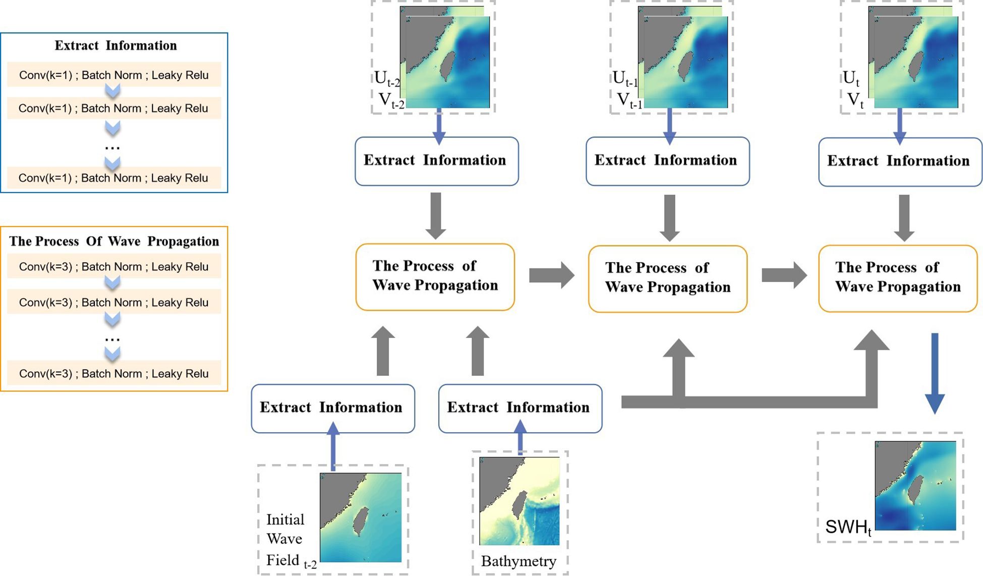
Figure 1 Schematic diagram of the NS prediction model based on convolutional neural networks.

Receptive field is an important consideration in handling pixel-level prediction problems, where rich contextual information in images significantly influences predictive performance, and such information is extracted through large receptive fields. In this study, the range of wave propagation module receptive fields is determined based on wave propagation, enabling the model to possess a reasonable range of perception for SWH prediction.

The PM spectrum (Pierson, 1964), which is derived from fully developed wind seas, is defined using two dimensionless parameters, α and β, expressed as follows (Equation 1):

$\begin{array}{ll}S(\omega )=\frac{\alpha g^2}{{\omega }^5}\exp [-\beta {(\frac{{\omega }_0}{\omega })}^4]& (1)\end{array}$

Wherein, $\alpha =8.1\times {10}^{-3},\beta =0.74,{\omega }_0=g/U$, and the corresponding peak frequency:

$\begin{array}{ll}{\omega }_p={(\frac{4}{5})}^{0.25}·\frac{g·{\beta }^{0.25}}{U}& (2)\end{array}$

In Equation (2), U is the wind speed at 19.5m above sea surface, g =9.81m/s² is the gravitational acceleration.

Additionally, the frequency ω satisfies the dispersion relation under deep water conditions, which states:

$\begin{array}{ll}{\omega }^2=gk& (3)\end{array}$

This relationship is related to the wave number k. By combining Equation (2) and Equation (3), the group velocity c_g is obtained, which is the propagation speed of wave energy at the peak frequency:

$\begin{array}{ll}{c}_g={\frac{\partial \omega }{\partial k}|}_{\omega ={\omega }_p}=\frac{1}{2}·\frac{U}{{(4/5)}^{0.25}·{\beta }^{0.25}}& (4)\end{array}$

Equation (4) represents the maximum propagation speed corresponding to the maximum wind speed.

The aforementioned deductions are based on the dispersion relations in deep water environments. As waves propagate from deep to shallow water, their speed is not only influenced by gravity and inertia but also by friction with the seabed and water pressure, leading to a gradual reduction in wave speed. Therefore, the maximum propagation speed in nearshore areas does not exceed that in deep water conditions.

The information extraction module utilizes 1x1 convolutional kernels to extract local information from each grid point, enhancing the non-linear expression capability of the output features. For the wave propagation module, we set the number of convolutional layers appropriately based on the maximum propagation distance of wave energy (see Section 4.1). Due to multiple inputs for the model, we add wind field and IWF together as well as concatenating them with bathymetry. This combination method is shown in Figure 2, which allows bathymetry data to engage deeply in the process of wave simulation at each moment. Therefore, it is beneficial for the network structure to be aligned with the physical process of wave propagation closely.

Figure 2

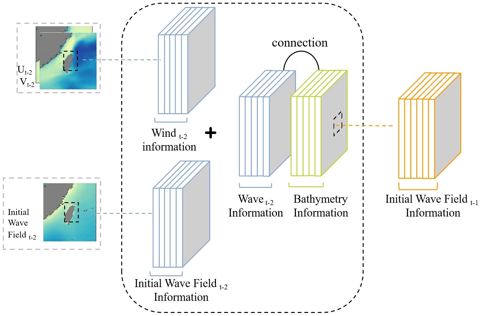
Figure 2 Method of combining different types of data.

2.3 Optimizer

As the input data is a regular square matrix containing both oceanic and terrestrial components, during the model training process, multiple layers of convolution may result in non-zero values near the ocean-land boundary, where the grid values originally representing the land portion may no longer be zero, thereby causing coastline misalignment. To ensure the accuracy of the coastline, a masking process is applied after each convolution and batch normalization, reassigning the land portion of all output channels to zero.

The model determines the direction for gradient descent by computing the discrepancy between the results and the labels, considering only the loss values from the marine parts to eliminate the impact of terrestrial regions on the experiments. The learning rate, which determines the magnitude of gradient descent, follows a dynamically changing scheme proposed in the formulas, varying from 1.0 to 0.1 as the number of epochs increases, thereby gradually reducing the learning rate (Equation 5).

$\begin{array}{ll}HuberLoss=\{\begin{array}{cc}\frac{\mathbf{1}}{\mathbf{2}}{(y_i-f(x_i))}^2,& \left|y_i-f(x_i)\right|\le \delta \\ \delta {(y_i-f(x_i))}^2-\frac{\mathbf{1}}{\mathbf{2}}{\delta }^2,& \left|y_i-f(x_i)\right|>\delta \end{array}& (5)\end{array}$

$\begin{array}{ll}\text{Loss}={{\displaystyle {\sum }_i^{I}HuberLoss}}_{\left\{\text{i}\in \text{Nearshore}\_\text{area}\right\}}& (6)\end{array}$

In Equation (6), “Nearshore_area” represents the nearshore study area, i denotes samples from the nearshore study area, and I represents the total number of sample points in the nearshore study area.

$\begin{array}{ll}\text{Learning Rate}=\frac{1}{2}(1+\cos (\frac{m\times \pi }{\text{Epoch}}))\times (1-0.01)+0.1& (7)\end{array}$

In Equation (7), Epoch represents the number of training iterations, and m indicates the current training iteration.

GWSM4C-NS was trained on a machine with NVIDIA GeForce RTX 3090 GPU (24 GB). The NS model was trained for 500 epochs, the batch size during training was set to 6.

2.4 Evaluation indicators

To appropriately evaluate our model, this paper selects a range of commonly used metrics for assessing the accuracy of SWH predictions. These include Differential Error (DR), Root Mean Square Error (RMSE), Mean Absolute Error (MAE), Mean Absolute Percentage Error (MAPE), and Correlation Coefficient (CC). MAE and MAPE quantify the proportionality of errors relative to the true label values, whereas RMSE measures the dispersion between the predicted values and the label values. The CC is used to assess the correlation between predicted values and label values. Due to the unique characteristics of the study marine areas, statistical calculations are performed exclusively for the nearshore regions. The mathematical equations for these evaluation metrics are as follows (Equations 8–12):

$\begin{array}{ll}\text{DR}(i,j)=\left|h_p(i,j)-h_m(i,j)\right|& (8)\end{array}$

$\begin{array}{ll}\text{MAE}=\frac{1}{I·J}{\displaystyle \sum _{i=1}^1{\displaystyle \sum _{j=1}^J\left|h_p(i,j)-h_m(i,j)\right|}}& (9)\end{array}$

$\begin{array}{ll}\text{MAPE}=\frac{100\%}{K·I·J}{\displaystyle \sum _{\text{k}=1}^K{\displaystyle \sum _{i=1}^I{\displaystyle \sum _{j=1}^J\frac{\left|h_p(i,j,k)-h_m(i,j,k)\right|}{h_m(i,j,k)}}}}& (10)\end{array}$

$\begin{array}{ll}\text{RMSE}=\frac{1}{K}{\displaystyle \sum _{\text{k}=1}^K\sqrt{\frac{1}{I·J}{\displaystyle \sum _{\text{i}=1}^I{\displaystyle \sum _{\text{j}=1}^J{(h_p(i,j,k)-h_m(i,j,k))}^2}}}}& (11)\end{array}$

$\begin{array}{ll}\text{CC}=\frac{{\displaystyle \sum _{k=1}^K(h_p(i,j,k)-\overline{h_p(i,j,k)})(h_m(i,j,k)-\overline{h_m(i,j,k)})}}{\sqrt{{\displaystyle \sum _{k=1}^K{(h_p(i,j,k)-\overline{h_p(i,j,k)})}^2}}·\sqrt{{\displaystyle \sum _{k=1}^K{(h_m(i,j,k)-\overline{h_m(i,j,k)})}^2}}}& (12)\end{array}$

where i and j denote the coordinates of space lattice points, k denotes cases, n represents the total number of cases, I denotes the total number of latitudinal lattice points, and J denotes the total number of meridional lattice points. DR(i,j) is the error value of a certain point in space, hp(i, j) is the SWH value predicted based on the model, and hm(i, j) is the MASNUM-WAM SWH value corresponding to a certain point in space, hp(i, j, k) represents the model-predicted SWH at a certain point in the case space, hp(i,j,k) represents the mean SWH predicted by the model at a certain point in the case space, and hm(i, j, k) represents the SWH of MASNUM-WAM at a certain point in the case space. hm(i,j,k) represents the mean SWH of MASNUM-WAM.

3 Results

3.1 Validation and analysis results from GWSM4C-NS

Figure 3 presents the seasonal average SWH for 2020 simulated by the MASNUM-WAM and GWSM4C-NS, along with the distribution of the DR between them. It can be observed that the GWSM4C-NS (Figures 3A-D) demonstrates good consistency in both the numerical values and spatial distribution of SWHs in nearshore areas compared to the results simulated by the MASNUM-WAM (Figures 3E-H). Figures 3I-L indicates most nearshore areas exhibit prediction errors less than 0.15m, with only some coastal and island areas showing relatively higher point-like distributed errors and the errors in autumn are higher than those in spring, summer, and winter. Additionally, the error distribution under different SWH is shown in Figure 4, the absolute error probability density under various SWHs displays a quasi-normal distribution. For SWHs between 0-1m, the probability density curve peaks sharply around zero, indicating a high accuracy in predictions for lower wave heights. As SWH increases (1-2m, 2-3m, and 3-4m), the curves maintain a quasi-normal distribution, with a slight shift to the right, suggesting an increase in the absolute error but still concentrated around low error values. The probability density curve for SWHs greater than 4m exhibits a broader spread and a lower peak, indicating a higher absolute error in predictions for larger wave heights. Overall, under conditions of low wave heights, the predictions tend to be smaller and the errors relatively minor, whereas at high wave heights, the errors are comparatively larger.

Figure 3

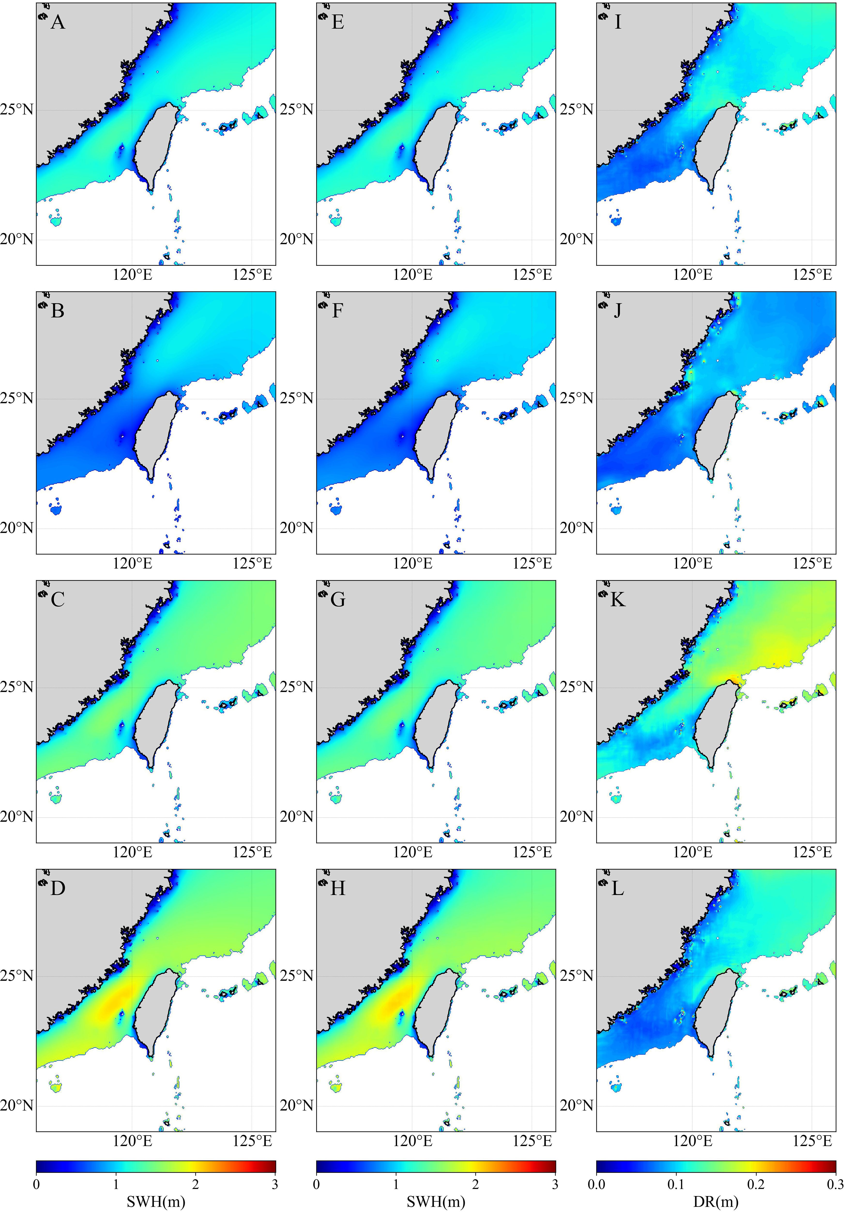
Figure 3 Comparison of simulation results between MASNUM-WAM and GWSM4C-NS. (A-D) GWSM4C-NS simulate SWH, (E-H) MASNUM-WAM simulate SWH, (I-L) DR of model predictions versus MASNUM -WAM simulation, for seasonal averages in spring (February, March, April), summer (May, June, July), autumn (August, September, October), and winter (November, December, January).

Figure 4

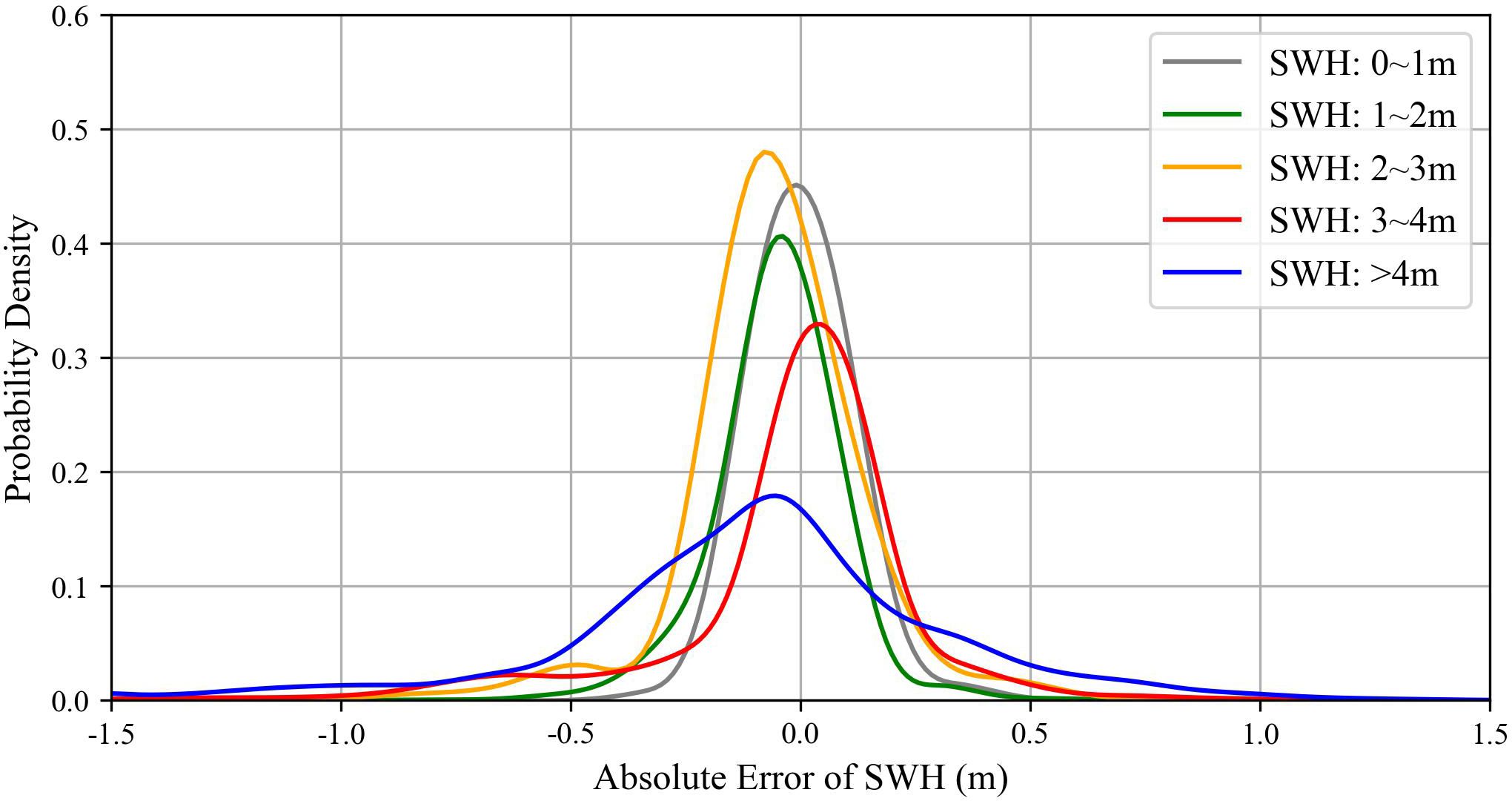
Figure 4 Probability density of absolute errors in SWH predictions across different SWH ranges. The SWH ranges are categorized as follows: 0-1m (gray), 1-2m (green), 2-3m (yellow), 3-4m (red), and greater than 4m (blue).

To verify the model’s improvement on the nearshore result of GWSM4C, i.e., the IWF data, we use the result of MASNUM-WAM as the target. Figures 5A-C displays the error and correlation coefficient between MASNUM-WAM and the GWSM4C, showing similar spatial distributions of RMSE (Figure 5A) and MAE (Figure 5B), particularly high near the depth of approximately 200m in the East Sea and surrounding coastal and island areas, while the CC (Figure 5C) shows the opposite (due to extremely high MAPE in coastal areas, reaching 100% or more, it is inconvenient to annotate contour lines and statistics, hence the MAPE of GWSM4C data is not displayed). Figures 5D-F displays the error and correlation coefficient between MASNUM-WAM and the NS model.

Figure 5

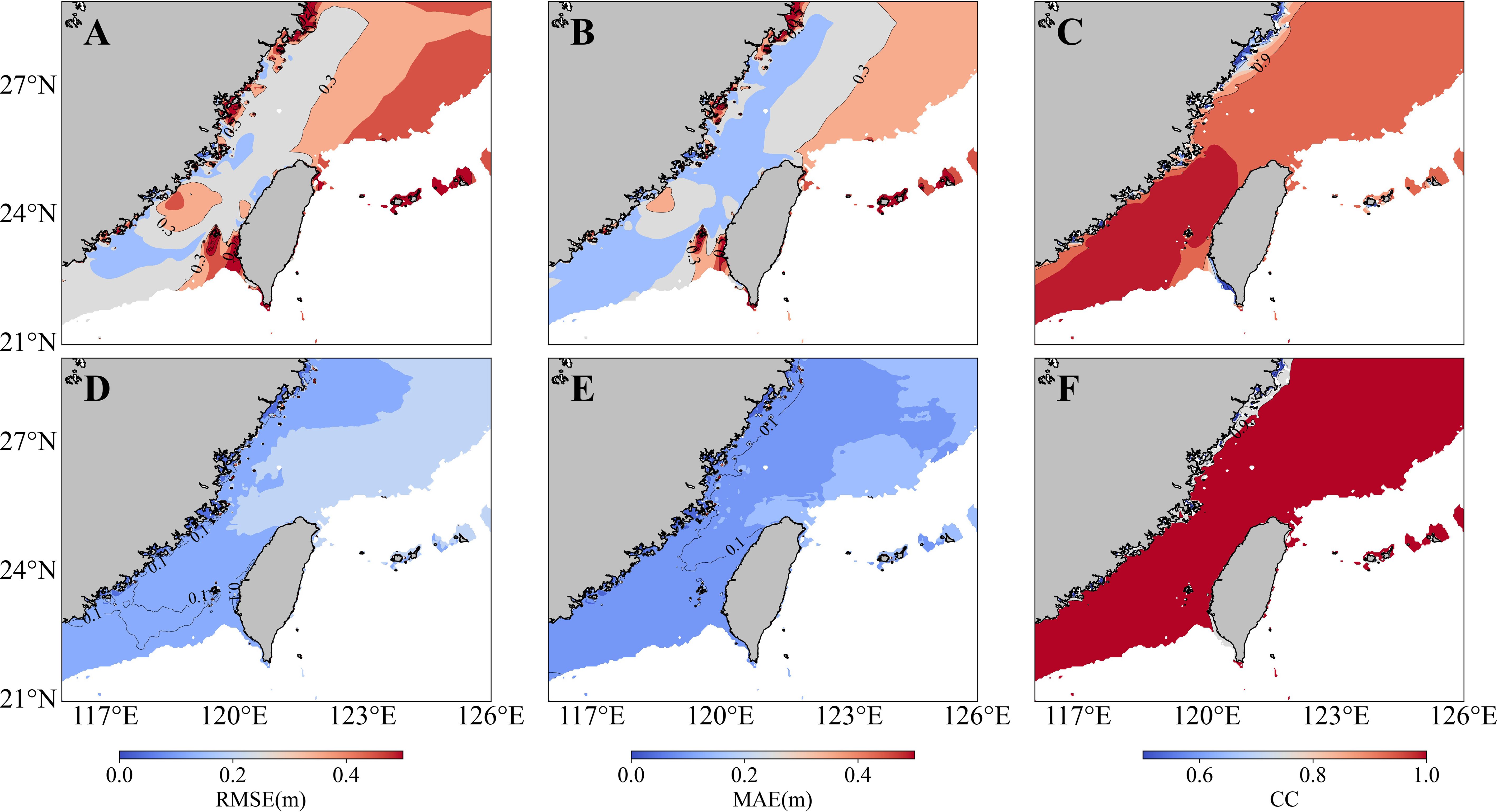
Figure 5 Annual mean contour distributions of (A) RMSE, (B) MAE, and (C) CC between MASNUM-WAM simulated SWH and GWSM4C model predicted SWH, Annual mean contour distributions of (D) RMSE, (E) MAE, and (F) CC between MASNUM-WAM and the GWSM4C-NS model.

3.2 Impact of bathymetry data on model predictions

Figure 6 quantifies the improvements in model simulation results based on GWSM4C data, with RMSE reduced from 0.312m to 0.128m, a 59% decrease; MAE reduced from 0.263m to 0.103m, a 60% decrease; and CC increased from 0.941 to 0.977. It can be observed that the predictions of the NS model show significant improvements compared to the GWSM4C. In contrast, Figure 7 highlights the impact of the NS without the inclusion of bathymetry data. Comparing this with the seasonal distribution data, it is evident that bathymetry data significantly enhance prediction accuracy, particularly in coastal and island regions. Statistical analysis reveals that incorporating bathymetry data reduces the RMSE of the model predicted SWH by 12%, decreases MAE by 11%, and increases the CC from 0.973 to 0.977.

Figure 6

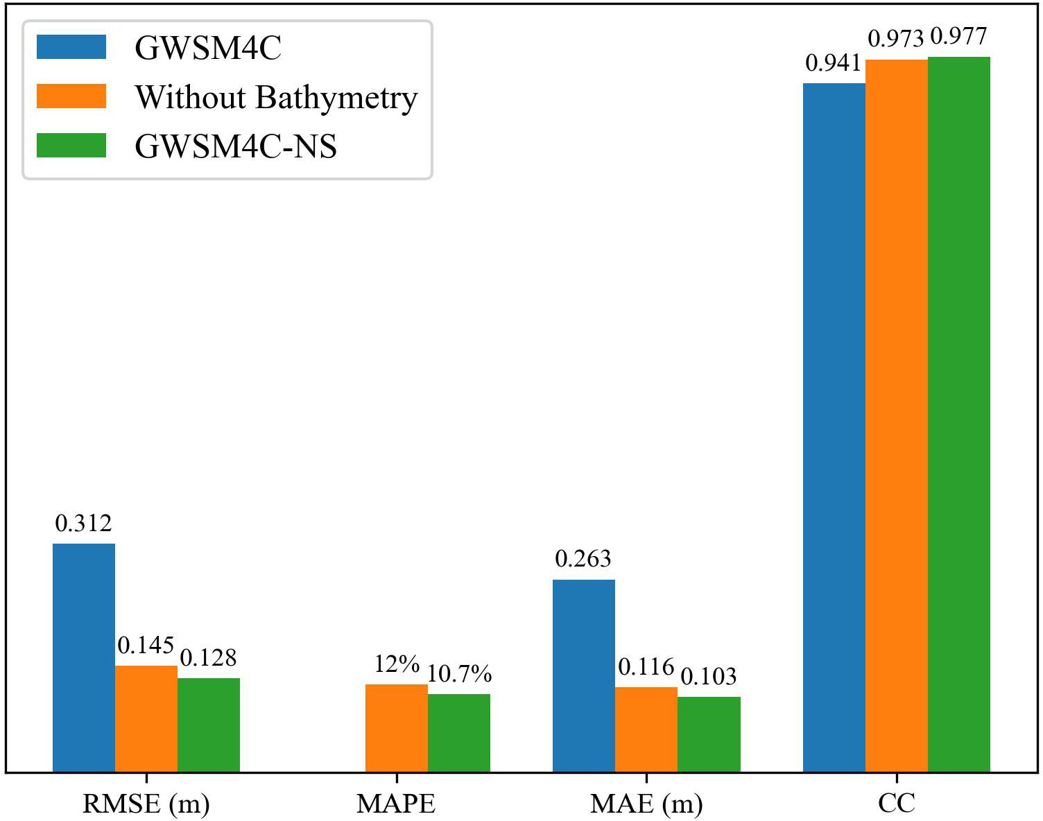
Figure 6 Annual mean statistics of RMSE, MAPE, MAE, and CC between GWSM4C, without bathymetry data input, and GWSM4C-NS model versus MASNUM-WAM simulation results.

Figure 7

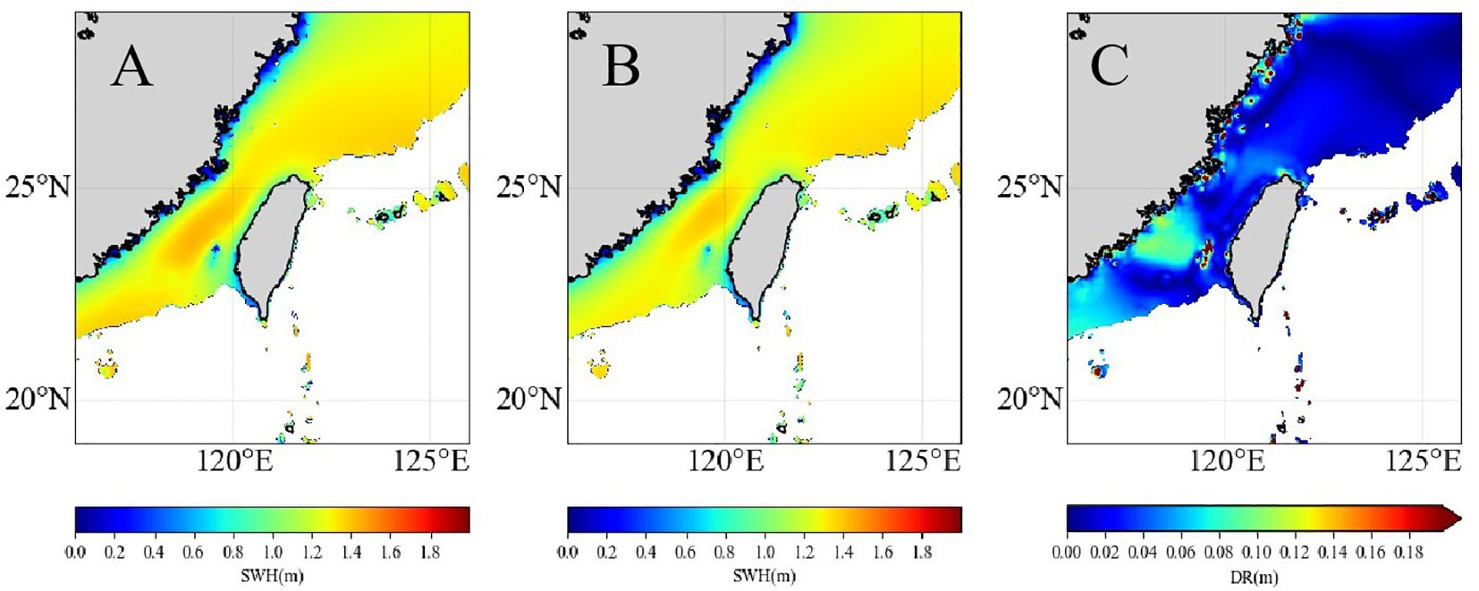
Figure 7 Comparison of simulation results between MASNUM-WAM and the GWSM4C-NS without Bathymetry data input. (A) MASNUM-WAM simulated SWH, (B) predicted SWH without Bathymetry data, (C) annual mean distribution of DR between Model prediction and MASNUM-WAM simulation.

4 Discussion

4.1 Effects of different convolution strategies

In this study, the maximum wind speed in the training dataset is 32 m/s (at 19.5m above sea level). According to the theoretical derivation of section 2.2, the maximum propagation speed of the waves is calculated to be 18.24 m/s. This implies that within a 1-hour interval, the farthest distance the waves can travel is approximately 65 km, which is equivalent to about 19 grids with a spatial resolution of 1/32°. Therefore, in the wave propagation simulation module, the maximum distance that the waves can travel per hour can be represented by setting the receptive field range to no less than 39.

We employ simulation experiments with three different sizes of convolutional kernels to determine the optimal scheme for accurately simulating nearshore SWH. As shown in Table 2, in all three experiments, the theoretical receptive field of each propagation module covers the maximum distance that waves can travel in one hour. Experiment 1 continuously uses 19 consecutive 3x3 small convolutional kernels; experiment 2 utilizes a network structure based on Hybird Dilated Convolution (HDC) (Lei et al., 2019) that effectively addresses the “grid artifacts” issue found in standard holey convolution models; Experiment 3 continuously uses 7 consecutive 7x7 convolutional kernels.

Table 2

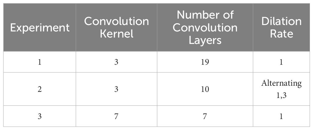
Table 2 Parameter settings for wave propagation schemes.

Figure 8 illustrates that the SWHs predicted by setups one (Figure 8A) and two (Figure 8B) are notably lower than those simulated by the MASNUM-WAM (Figure 8D), especially in the Taiwan Strait area, whereas the predictions of setup three (Figure 8C) closely align with the MASNUM-WAM in terms of numerical values. Table 3 demonstrates that setup three achieves the best statistical performance, with an RMSE of 0.128m, a MAPE of 10.7%, and an MAE of 0.103m, which are the lowest among all setups. Additionally, setup three attains the highest CC of 0.977. Given its superior numerical predictions, the network structure of experiment 3 is selected for the propagation module in this paper.

Figure 8

Figure 8 Annual mean statistical results of SWH simulation for different schemes (A) Experiment 3, (B) Experiment 2, (C) Experiment 3, (D) MASNUM-WAM.

Table 3

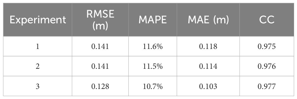
Table 3 Statistical results of prediction for different wave propagation schemes.

4.2 Suitability of non-training areas

The GWSM4C-NS model proposed in this paper is based on the wave propagation mechanisms, theoretically endowing it with a certain degree of regional generalization capability. We selected the coastal area ranging from 111°E to 118°E and from 18°N to 25°N (referred to as Area 2) for testing. We discussed the predictive capability of the model in non-training areas, which further validates the model’s ability to learn about wave propagation processes. Figure 9 illustrates the seasonal average SWH in 2018 simulated by the MASNUM-WAM (Figures 9E-H) and the GWSM4C-NS model (Figures 9A-D) within Area 2, as well as the DR between the two. It is evident that the model demonstrates good consistency in the predicted SWH values and spatial distribution compared to the MASNUM-WAM simulation results in the nearshore areas, although the predicted values are slightly underestimated. Statistical analysis (as shown in Figures 10, 11) reveals that in Area 2, the RMSE, MAPE, MAE, and CC between the model predictions and MASNUM-WAM simulations are 0.161m, 12.9%, 0.137m, and 0.951, respectively. The RMSE and MAE have decreased by 43% and 39% compared to the predictions by the GWSM4C model. This signifies an improvement in the prediction of nearshore SWH based on the GWSM4C model.

Figure 9

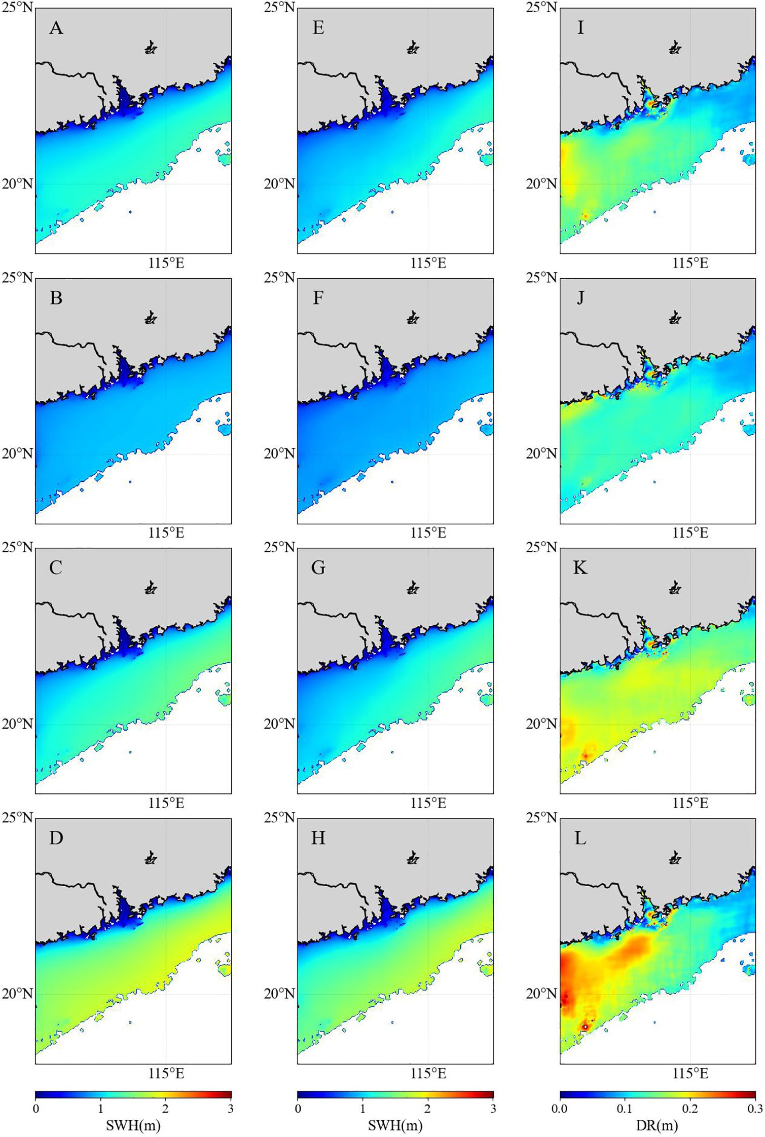
Figure 9 Comparison of simulation results between MASNUM-WAM and the NS model in area 2. (A-D) GWSM4C-NS Model-Predicted SWH, (E-H) MASNUM-WAM simulated SWH, (I-L) DR between model predictions and MASNUM-WAM predictions for seasonal averages in spring (February, March, April), summer (May, June, July), autumn (August, September, October), and winter (November, December, January).

Figure 10

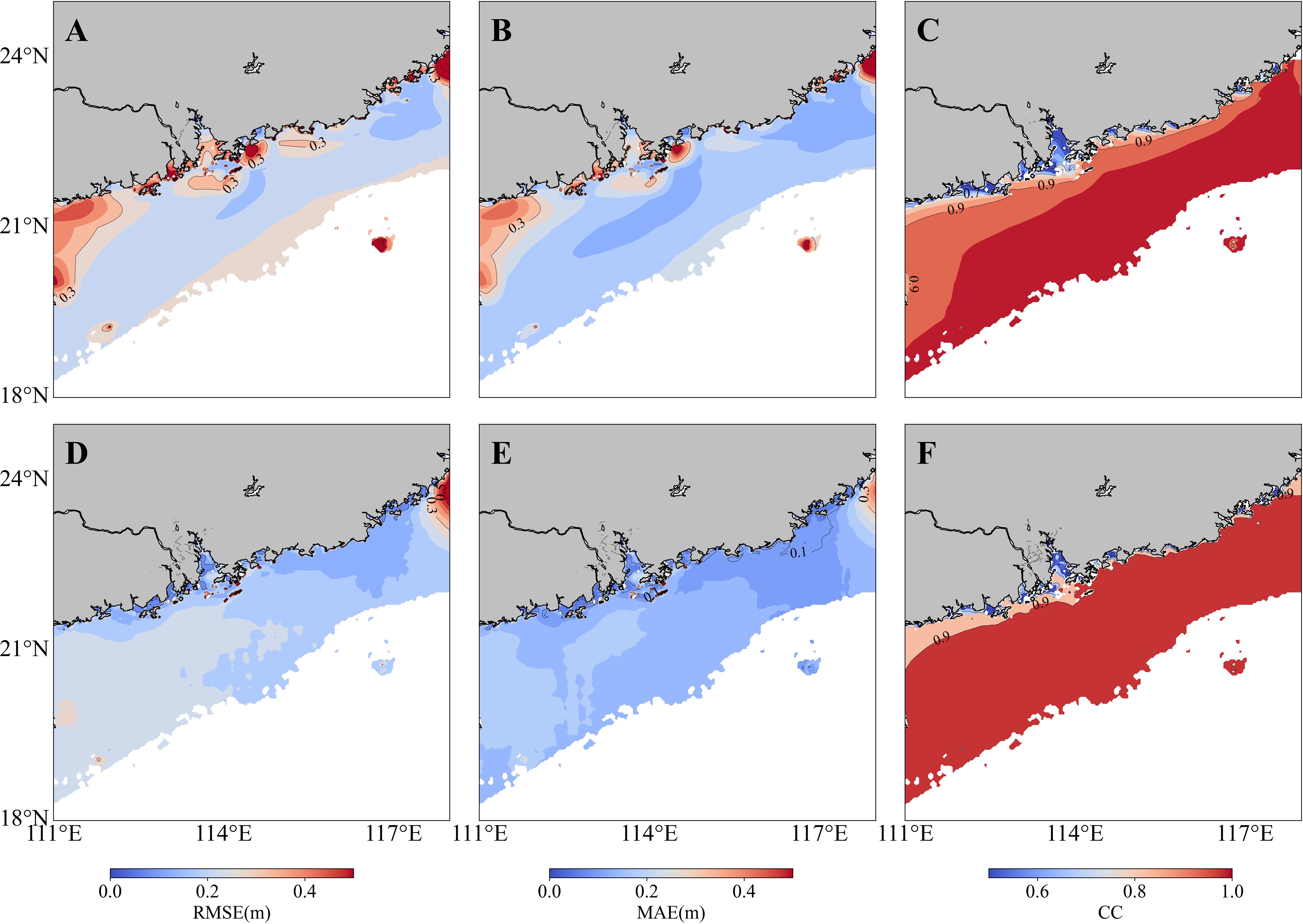
Figure 10 Annual mean contour distributions of (A) RMSE, (B) MAE, and (C) CC between MASNUM-WAM simulated SWH and GWSM4C model predicted SWH, Annual mean contour distributions of (D) RMSE, (E) MAE, and (F) CC between MASNUM-WAM and the GWSM4C-NS model in area2.

Figure 11

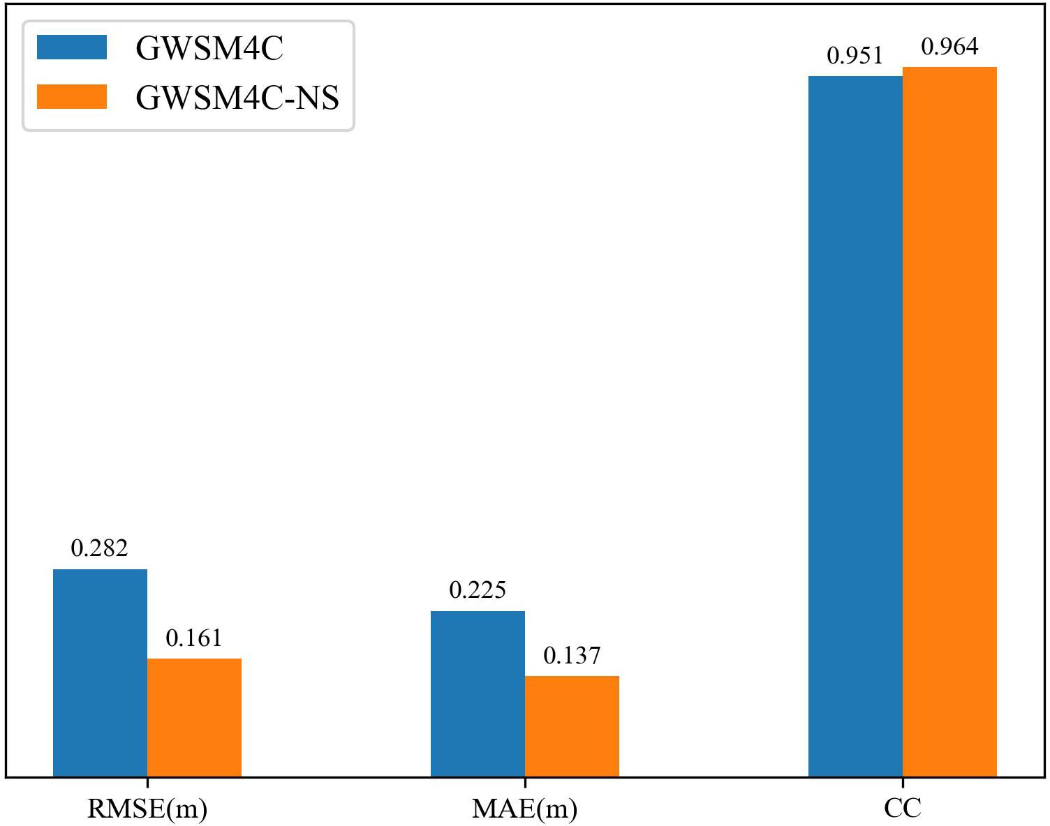
Figure 11 Annual mean statistics of RMSE, MAE, and CC between GWSM4C, the GWSM4C-NS model results, and MASNUM-WAM simulation results.

Therefore, the physically based NS model proposed in this paper is capable of predicting in untrained areas, saving the computational time and resources required for training.

5 Conclusion

In recent years, deep learning has been widely applied in the field of wave prediction. Compared to the widely used neural networks that combine convolutional and recurrent elements, pure convolutional neural networks are less prone to the accumulation of errors over time. The recently published GWSM4C model can update initial conditions simultaneously as the simulation is going on, thus, the accumulation of errors from a fixed initial wave state can be avoided, and long-term simulation based on deep learning algorithms become possible. Building upon the foundation of GWSM4C, the newly proposed GWSM4C-NS model incorporates the effects of water depth on wave propagation, yielding more accurate SWH in nearshore regions. The “Results” section demonstrates the test results, and the conclusions are as follows:

1.Compared to networks using 3×3 convolution kernels and dilated convolutions based on the HDC framework, the network structure with 7×7 convolution kernels provide a more accurate simulation of the wave propagation process. Additionally, bathymetry data in nearshore areas can improve the accuracy of predicted SWH, specially in regions around islands and coasts.

2. Compared to the MASNUM-WAM simulation results, the prediction results of the NS model show RMSE, MAPE, MAE, and CC values of 0.128m, 10.7%, 0.103m, and 0.977, respectively. And further comparison with the original GWSM4C predictions, the RMSE and MAE are reduced by 59% and 60%, respectively. Therefore, the new NS model can effectively improve the performance of GWSM4C in nearshore areas.

3. The NS model can also conduct predictions in other untrained sea areas. Although the prediction results in the untrained region might be not as accurate as those in the trained one, they still achieve an acceptable level of agreement with the MASNUM-WAM’s outputs.

Data availability statement

The data that support the findings of this study are available on request from the corresponding author: QJ 21qjin@stu.edu.cn .

Author contributions

HZ: Writing – original draft. QJ: Writing – review & editing. FH: Writing – review & editing. ZW: Writing – original draft.

Funding

The author(s) declare financial support was received for the research, authorship, and/or publication of this article. This work was supported by the National Key Research and Development Program of China (2022YFC3104801), the Shantou University Scientific Research Funded Project (NTF21036), and the Open Research Fund of Guangdong Provincial Key Laboratory of Marine Disaster Prediction and Prevention (GPKLMD2023005).

Acknowledgments

We appreciate the reviewers for their comments and suggestions, which helped to improve the quality of this manuscript.

Conflict of interest

The authors declare that the research was conducted in the absence of any commercial or financial relationships that could be construed as a potential conflict of interest.

Publisher’s note

All claims expressed in this article are solely those of the authors and do not necessarily represent those of their affiliated organizations, or those of the publisher, the editors and the reviewers. Any product that may be evaluated in this article, or claim that may be made by its manufacturer, is not guaranteed or endorsed by the publisher.

References

Cao H., Liu G., Huo J., Gong X., Wang Y., Zhao Z., et al. (2023). Multi factors-PredRNN based significant wave height prediction in the Bohai, Yellow, and East China Seas. Front. Mar. Sci. 10. doi: 10.3389/fmars.2023.1197145

CrossRef Full Text | Google Scholar

Fan S., Xiao N., Dong S. (2020). A novel model to predict significant wave height based on long short-term memory network. Ocean Eng. 205, 107298. doi: 10.1016/j.oceaneng.2020.107298

CrossRef Full Text | Google Scholar

Han L., Ji Q., Jia X., Liu Y., Han G., Lin X. (2022). Significant wave height prediction in the South China sea based on the convLSTM algorithm. J. Mar. Sci. Eng. 10 (11), 1683. doi: 10.3390/jmse10111683

CrossRef Full Text | Google Scholar

Hu H., van der Westhuysen A. J., Chu P., Fujisaki-Manome A. (2021). Predicting Lake Erie wave heights and periods using XGBoost and LSTM. Ocean Model. 164, 101832. doi: 10.48550/arXiv.1912.01786

CrossRef Full Text | Google Scholar

Jin Q., Hua F., Yang Y. (2019). Prediction of the significant wave height based on the support vector machine. Adv. Mar. sci. 37, 199–209. doi: 10.3969/j.issn.1671-6647.2019.02.004

CrossRef Full Text | Google Scholar

Jin Q., Jiang X., Hua F., Yang Y., Jiang S., Chen Y., et al. (2024). GWSM4C: A global wave surrogate model for climate simulation based on a convolutional architecture. Ocean Eng. 309, 118458. doi: 10.1016/j.oceaneng.2024.118458

CrossRef Full Text | Google Scholar

Kim J., Kim T., Yoo J., Ryu J., Do K., Kim J. (2022). OceanWaveNet: Spatio-temporal geographic information guided ocean wave prediction network. Ocean Eng 257, 111576. doi: 10.1016/j.oceaneng.2022.111576

CrossRef Full Text | Google Scholar

Lei X., Pan H., Huang X. (2019). A dilated CNN model for image classification. IEEE Access 7, 124087–124095. doi: 10.1109/ACCESS.2019.2927169

CrossRef Full Text | Google Scholar

Londhe S. N. (2008). Soft computing approach for real-time estimation of missing wave heights. Ocean Eng. 35, 1080–1089. doi: 10.1016/j.oceaneng.2008.05.003

CrossRef Full Text | Google Scholar

Mahjoobi J., Mosabbeb E. A. (2009). Prediction of significant wave height using regressive support vector machines. Ocean Eng. 36.5, 339–347. doi: 10.1016/j.oceaneng.2009.01.001

CrossRef Full Text | Google Scholar

Makarynskyy O. (2004). Improving wave predictions with artificial neural networks. Ocean Eng. 31, 709–724. doi: 10.1016/j.oceaneng.2003.05.003

CrossRef Full Text | Google Scholar

Pierson W. J. (1964). A proposed spectral form for fully developed wind seas based on the similarity theory of S. A. Kitaigorodskii. J. Geophys. Res. 69 (24), 5181–5190. doi: 10.1029/JZ069i024p05181

CrossRef Full Text | Google Scholar

Qu Y., Gao Z., Cai J., Wang J., Hou F. (2022). Comparison of wave prediction ability between numerical model and AI model. Mar. Forecasts 39, 17–26. doi: 10.11737/j.issn.1003-0239.2022.05.003

CrossRef Full Text | Google Scholar

Shi X., Chen Z., Wang H., Yeung D.-Y., Wong W.-K., Woo W.-c. (2015). Convolutional lstm network: A machine learning approach for precipitation nowcasting. Adv. Neural Inf. Process. Syst. 1, 802–810. doi: 10.48550/arXiv.1506.04214

CrossRef Full Text | Google Scholar

Song W., Zhou X., Bi F., Guo D., Gao S., He Q., et al. (2009). Automatic wave height detection from nearshore wave videos. Int. J. Image Graph. 25, 0507–0519. doi: 10.11834/jig.190138

CrossRef Full Text | Google Scholar

Wang L., Deng X., Ge P., Dong C., J. Bethel B., Yang L., et al. (2022). CNN-biLSTM-attention model in forecasting wave height over south-east China seas. Comput. Mater. Contin. 73 (1), 2151–2168 doi: 10.32604/cmc.2022.027415

CrossRef Full Text | Google Scholar

Waseda T., In K., Kiyomatsu K., Tamura H., Miyazawa Y., Iyama K. (2014). Predicting freakish sea state with an operational third-generation wave model. Nat. Hazard Earth Sys. 14, 945–957. doi: 10.5194/nhess-14-945-2014

CrossRef Full Text | Google Scholar

Waseda T., Tamura H., Kinoshita T. (2012). Freakish sea index and sea states during ship accidents. J. Mar. Sci. Tech. 17, 305–314. doi: 10.1007/s00773-012-0171-4

CrossRef Full Text | Google Scholar

Wei J., Malanotte-Rizzoli P., Eltahir A., B. E., Xue P., Xu D. (2013). Coupling of a regional atmospheric model (RegCM3) and a regional oceanic model (FVCOM) over the maritime continent. Clim Dynam. 43, 1575–1594. doi: 10.1007/s00382-013-1986-3

CrossRef Full Text | Google Scholar

Yuan Y., Hua F., Pan Z., Sun L. (1991). LAGDF-WAM numerical wave model—I. basic physical model. Acta Oceanol. Sin. 10, 4.

Google Scholar

Yuan Y., Hua F., Pan Z., Sun L. (1992). LAGFD-WAM numerical wave model—II: characteristics inlaid scheme and its application. Acta Oceanol. Sin. 11, 1.

Google Scholar

Zhou S., Xie W., Lu Y., Wang Y., Zhou Y., Hui N., et al. (2021). ConvLSTM-based wave forecasts in the south and east China seas. Front. Mar. Sci. 8. doi: 10.3389/fmars.2021.680079

CrossRef Full Text | Google Scholar