 Anna Marcout
 Eric Foucher2
 Graham J. Pierce
- 1Normandie Université, UNICAEN, Alliance Sorbonne Université, MNHN, UA, CNRS, IRD, Biologie des Organismes et Ecosystèmes Aquatiques (BOREA), Esplanade de la Paix, Caen, France
- 2Ifremer, Laboratoire Ressources Halieutiques, Port-en-Bessin, France, France
- 3Departamento de Ecologia y Recursos Marinos, Instituto de Investigaciones Marinas (CSIC), Vigo, Spain
The English Channel has the highest long-finned squid landings in the Northeast Atlantic, making squid one of the most valuable resources exploited by demersal fisheries operating in this area. This resource consists of two short-lived long-finned squid species: Loligo forbesii and L. vulgaris, which have a similar appearance (they are not distinguished by fishers) but differ in the timing of their life cycle: in L. forbesii, the recruitment peak occurs in July while in L. vulgaris recruitment peak occurs in November. The abundance and distribution of cephalopod species, such as Loligo spp., depends on favourable environmental conditions to support growth, reproduction and successful recruitment. This study investigated the role of several environmental variables (bottom temperature, salinity, current velocity, phosphate and chlorophyll concentrations) on recruitment biomass (in July for L. forbesii and November for L. vulgaris), as based on environmental data for pre-recruitment period from the Copernicus Marine Service and commercial catches of French bottom trawlers during the recruitment period over the years 2000 to 2021. To account for non-linear relationship between environmental descriptors and the biological response, General Additive Models (GAM) were fitted to the data. Separate models were obtained to forecast L. vulgaris and L. forbesii biomass indices during their respective recruitment periods. These models explain a high percentage of variation in biomass indices (65.8% for L. forbesii and 56.7% for L. vulgaris) and may be suitable to forecast the abundance (in terms of biomass) and spatial distribution of the resource. Such forecasts are desirable tools to guide fishery managers. Since these models can be fitted shortly before the start of the fishing season, their routine implementation would take place in real-time fishery management (as promoted by fishery scientists dealing with short-lived species).
1 Introduction
Due to their particular ecological characteristics (short life-span, semelparity and rapid growth), squid are set apart from many other commercial exploited species. Their population dynamics display high variability because abundance and fishing yields depend almost entirely on recruitment success of the annual cohort (Caddy, 1983; Pierce and Guerra, 1994; Arkhipkin et al., 2015; Doubleday et al., 2016: Moustahfid et al., 2021).
In short-lived animals such as squid, recruitment is highly driven by environmental factors through influences on adult fecundity, egg quality, hatching success, and growth and mortality of paralarvae and juveniles (Caddy, 1983; Fogarty, 1989; Dawe et al., 2007; Pierce et al., 2008, 2010; Rodhouse et al., 2014; Bruggeman et al., 2022; Suca et al., 2022). A better understanding of the environmental influences on recruitment and hence interannual variability would enable pre-recruitment predictions of likely stock size in the coming season (Arkhipkin et al., 2015; Moustahfid et al., 2021).
The English Channel has the highest long-finned squid landings of any area in the Northeast Atlantic, making it an important fishing ground for squid for both French and UK trawlers (ICES, 2020). This resource consists of two short-lived long-finned squid species (not distinguished by fishers): veined squid Loligo forbesii and European squid Loligo vulgaris (Royer, 2002). Loligo forbesii is distributed from North European waters as far north as the Faroe Islands to Northwest Africa and the Mediterranean Sea (Holme, 1974). Loligo vulgaris shares the southern part of this range and predominates in Atlantic waters of the Iberian Peninsula and in the Mediterranean (Guerra and Rocha, 1994; Moreno et al., 2002), while being almost completely absent from Scottish waters (Pierce et al., 1994b, 1998). Loligo forbesii usually spawns in slightly deeper waters than does L. vulgaris, usually between 10 and 150 m (occasionally at 300–500 m, and even as deep as ~700m; Lordan and Casey, 1999); L. vulgaris spawns mostly in water depths of under 50 m (Jereb et al., 2015).
Despite the fact that the two species are not reported separately in landings, we are able to study recruitment peaks separately because the two species differ in the timing of their life cycle. Sampling of squid landings at Port-en-Bessin fish market (1993-today; Royer, 2002; ICES, 2016 and ICES, 2020) shows that young L. forbesii individuals appear in June, when L. vulgaris are rare (less than 1%), with the highest number of recruits (the smallest fished animals) seen in July. Loligo vulgaris individuals gradually appear in the nets from September onwards, with recruits (the smallest animals) reaching over 80% of the animals sampled from landings in November. These observations have enabled us to consider two distinct recruitment peaks to study the two species separately: in July for L. forbesii and November for L. vulgaris.
Life cycle and growth are relatively poorly understood mainly because of the similarity of the young forms of the two co-occuring species (Jereb et al., 2015). In the English Channel, spawning seems to occur around seven months before the recruitment of new cohort; around December for L. forbesii and around April for L. vulgaris when the individuals are at their largest (Challier et al., 2005; Laptikhovsky et al., 2022) suggesting that females are ready to lay their eggs just before dying. In Loligo species, embryonic development lasts from a few weeks to a few months (Villanueva et al., 2003). For L. forbesii, the egg development spans 68 to 75 days at 12.5°C (Segawa et al., 1988), while for L. vulgaris, it ranges from 45–70 days at 12–14°C (Mangold-Wirz, 1963; Boletzky, 1979). This is followed by 2–3 months of life as planktonic paralarvae (Craig, 2001). Due to the variability of reproductive and growth parameters, the pre-recruitment period (4, 5, 6 and 7 months before recruitment) seems to be the most sensitive period in terms of influencing recruitment.
In short-lived species such as cephalopods, in which environmental factors play a crucial role in recruitment and hence in determining annual abundance, the implementation of stock assessment is generally difficult (Pierce and Guerra, 1994; Guerra et al., 2010; Arkhipkin et al., 2021; Moustahfid et al., 2021). Because population size varies seasonally, depending on when it is measured it may or may not be an accurate indicator of recruitment the following year (Caddy, 1983; Boyle, 2002; Pierce and Boyle, 2003). Information about the potential size of the exploitable stock will only become available shortly before recruitment (Roa-Ureta and Arkhipkin, 2007). Based on the high sensitivity of cephalopod abundance to environmental conditions and the fact that there is often only one cohort per year, squid abundance could arguably be predicted from environmental conditions alone (Pierce and Guerra, 1994; Pierce et al., 2008; Arkhipkin et al., 2021).
Currently, no quotas apply to squid fishing in the English Channel. Under the Common Fisheries Policy of the European Union (EU-CFP) no assessment programs have been established for assessing cephalopod stocks in European waters. Most stock assessment methods are applied retrospectively, which is of limited value in such short-lived species with weak stock-recruitment relationships (e.g. Caddy, 1983) while real-time assessment requires intensive (and expensive) monitoring and must be accompanied by in-season management (Arkhipkin et al., 2021). Therefore, forecasting offers the most plausible option to inform management of this resource, as is becoming increasingly necessary in the context of increasing anthropogenic pressures (e.g., climate change, overfishing).
The objective of the present study was to investigate how recruitment biomass indices (in July for L. forbesii and in November for L. vulgaris) were influenced by environmental variables during the pre-recruitment period in the English Channel, using Generalised Additive Models (GAM) with time-lagged effects. The models not only quantified environmental effects during the pre-recruitment period but also provided predictions of biomass distribution and recruitment strength for the two species that could assist managers in advising on the exploitation of the resources.
2 Materials and methods
2.1 English Channel data sources
2.1.1 Recruitment biomass indices
For biomass indices, we used landings (kg) per unit effort (hours of trawling) (LPUE) from 2000 to 2021 for all French bottom otter trawls (OTB) in each ICES statistical rectangle of the English Channel. These data were collected from national databases (Système d’Information Halieutique-SIH) managed by Ifremer.
We applied a vector autoregressive spatio-temporal (VAST) model implemented using the R package “VAST” (https://github.com/James-Thorson-NOAA/VAST) (Thorson, 2019) to standardize LPUE by month from 2000 to 2021 (264 months in total) and by rectangle. The advantage of using this delta-glm model is that it accounts for both the probability of encounter and the (positive) catch rate when squid are encountered and allows the integration of co-variables that influence biomass or catches (e.g. vessel power). The computation of biomass indices is similar to what is explained in the preprint by Marcout et al. (2024).
As the two loliginid species differ in the timing of their life cycles (Royer, 2002; Laptikhovsky et al., 2022), biomass indices in July are considered for L. forbesii recruitment peak and biomass indices in November are considered for L. vulgaris recruitment peak (Figure 1; Robin and Boucaud-Camou, 1995; Royer, 2002; Challier et al., 2005).
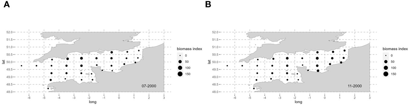
Figure 1 Squid biomass indices in the English Channel in 2000 for L. forbesii recruitment in July (A) and for L. vulgaris recruitment in November (B) for each ICES statistical rectangle. Maps for other years (2001–2021) can be found in the Supplementary Material (Appendix 1).
2.1.2 Environmental data
Ten candidate variables were extracted from EU’s Copernicus Marine Environment Monitoring Service (CMEMS) (https://marine.copernicus.eu/) as monthly means (Table 1): sea bottom temperature (bottomT), sea surface salinity (so), eastward sea water velocity (uo), northward sea water velocity (vo), net primary production (nppv), molar concentration of nitrate (no3), molar concentration of phosphate (po4) and concentration of chlorophyll a (chl).
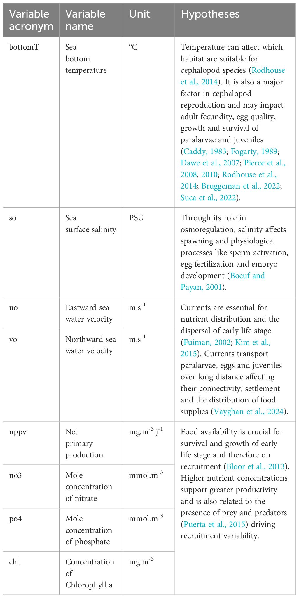
Table 1 Summary of the candidate variables included in this study and detailed hypotheses relating them to recruitment success.
The spatial resolution of the model for grid data was 0.111° × 0.067° (approximately 7 km horizontal resolution). We linked each geographical coordinate to an ICES rectangle and computed the average value of each variable per rectangle and per month.
To understand the spatial distributions of the resource and their associated environmental conditions, longitude and latitude of each ICES rectangle (geographical coordinate of its barycenter) were selected as spatial factors. Including these spatial factors enhances the predictive power of ecological models by accounting for unmeasured or unobserved processes (Legendre, 1993; Brodie et al., 2020). By focusing on latitude and longitude rather than other abiotic factor such as depth, our model captures a broader range of processes and enhance predictive accuracy through the direct incorporation of spatial dynamics (Araújo et al., 2019).
To identify the relationships between recruitment biomass indices (in July for L. forbesii and November for L. vulgaris) and hydro-climatic parameters during the pre-recruitment period (which corresponds to the egg incubation and juvenile stages), we have selected environmental factors 4, 5, 6 and 7 months before the recruitment for each of the two species.
2.2 Data analysis
2.2.1 Recruitment peak patterns
To confirm the consistent seasonal recruitment pattern for both species as suggested by Royer et al. (2002), we examined the month preceding and following the recruitment peak for both species to determine if there are any annual recruitment discrepancies. For both species, we assessed the correlations between the recruitment biomass index and the biomass indices from the preceding and subsequent months over the period from 2000 to 2021. Normality was checked with Shapiro-Wilk normality test. If the data followed a normal distribution and were homoscedastic, Pearson’s correlation test were conducted otherwise Spearman’s correlation test were conducted.
2.2.2 GAM fitting procedures
Because we cannot assume linear relationships between biomass indices and explanatory variables, Generalized Additive Models (GAM) were used (Hastie and Tibshirani, 1990; Lehmann et al., 2002; Murase et al., 2009).
Before fitting a model to the data, we examined monthly time series of environmental predictors on the whole English Channel from 2000 and 2021 to identify relationships among these predictors. values of the Variance Inflation Factor (VIF) were were used to explore multicollinearity of variables during the pre-recruitment period (4, 5, 6 and 7 months before the recruitment for each of the two species). Variables with a VIF value greater than 10 are considered highly correlated and were removed (Neter et al., 1996; Chatterjee et al., 2000; Han et al., 2022).
In total, 8 models were fitted (Table 2).

Table 2 Description of the 8 models fitted.
The general form of GAM models used in the analysis assuming a Gaussian distribution has the following structure:
where BI is the recruitment biomass index (in July for L. forbesii and November for L. vulgaris) for each rectangle and each year; s is the smoothing function (with k ≤ 6 to avoid overfitting), s(x) represents the effect of each environmental factors in the pre-recruitment period (for each statistical rectangle and year) and s(lat,lon) represents the influence of spatial factors (i.e. latitude, longitude and their interaction for each rectangle). Spatial factors can serve as proxies for unmeasured or unexplained processes due to spatial autocorrelation of environmental factors (Brodie et al., 2020).
Response variables (biomass indices in July and November) were log transformed to conform to the model assumption of normal distribution. Using forward selection, the Akaike information criterion (AIC) was used to measure the goodness of fit of the models, where the smaller the AIC value, the better the model fit (although models which differ in AIC by less than two units may be considered equivalent). It is calculated as follows:
where k denotes the number of independent parameters of the model and L denotes the maximum likelihood function of the model. The model’s stability was assessed through 10-fold cross validation, and the RMSE value of each model was calculated to assess the performance of the models.
The models obtained were tested with the data from the final three years (2019–2021), which were not included to build the model (2000–2018). The gam.check() function was run for each model to produce basic residual plots and information about the fitting process and potential violation to statistical assumptions (Wood, 2006).
All statistical analyses were carried out in R using the GAM functions of the “mgcv” package (Wood, 2006; R Development Core, 2023).
3 Results
3.1 Recruitment biomass indices
First, interannual variability of recruitment biomass indices was investigated in July for L. forbesii and in November for L. vulgaris over all ICES rectangles in the English Channel between 2000 and 2021 (Figure 2).
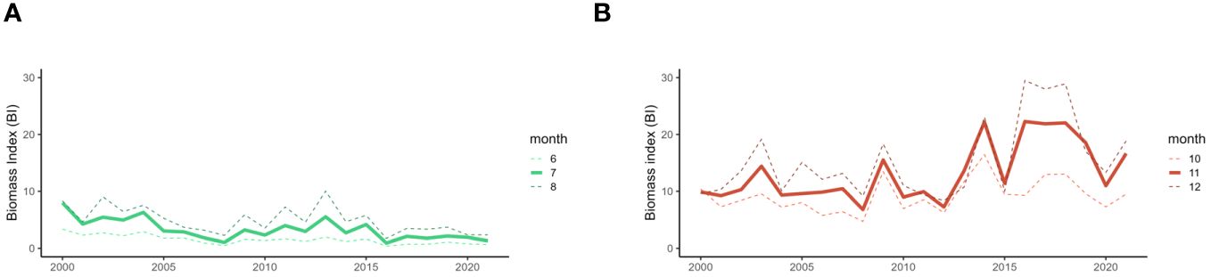
Figure 2 The monthly average squid biomass indices in the English Channel in July (A) for L. forbesii and in November (B) for L. vulgaris and the biomass indices from the preceding and subsequent months between 2000 and 2021.
The recruitment biomass indices for L. forbesii in July and L. vulgaris in November follow the biomass trends observed in the preceding and following months suggesting a consistent seasonal recruitment pattern for both species. In July, the recruitment biomass for L. forbesii is significantly and positively correlated with June indices (r=0.96, p<0.001) and August indices (r=0.90, p<0.001). Similarly, the recruitment biomass of L. vulgaris in November showed a significant positive correlation with the October (r=0.79, p<0.001) and December indices (r=0.83, p<0.001).
In relation to interannual trends, biomass indices in July gradually decreased from an average of 8 in 2000 to an average of 1 in 2021 suggesting a decrease of recruitment biomass peak for L. forbesii. Biomass indices in November seem to have been stable from 2000 to 2014 around 10 with highs around 15 in 2004 and 2009. There was a general increase from 2014 to 2021, reaching values of 22 in 2014, 2016, 2017 and 2018 suggesting an increase of recruitment biomass peak for L. vulgaris since 2014.
3.2 Environmental trends in the English Channel
To identify relationships between environmental predictors, monthly time series were analyzed for the whole English Channel from 2000 to 2021 (Figure 3).
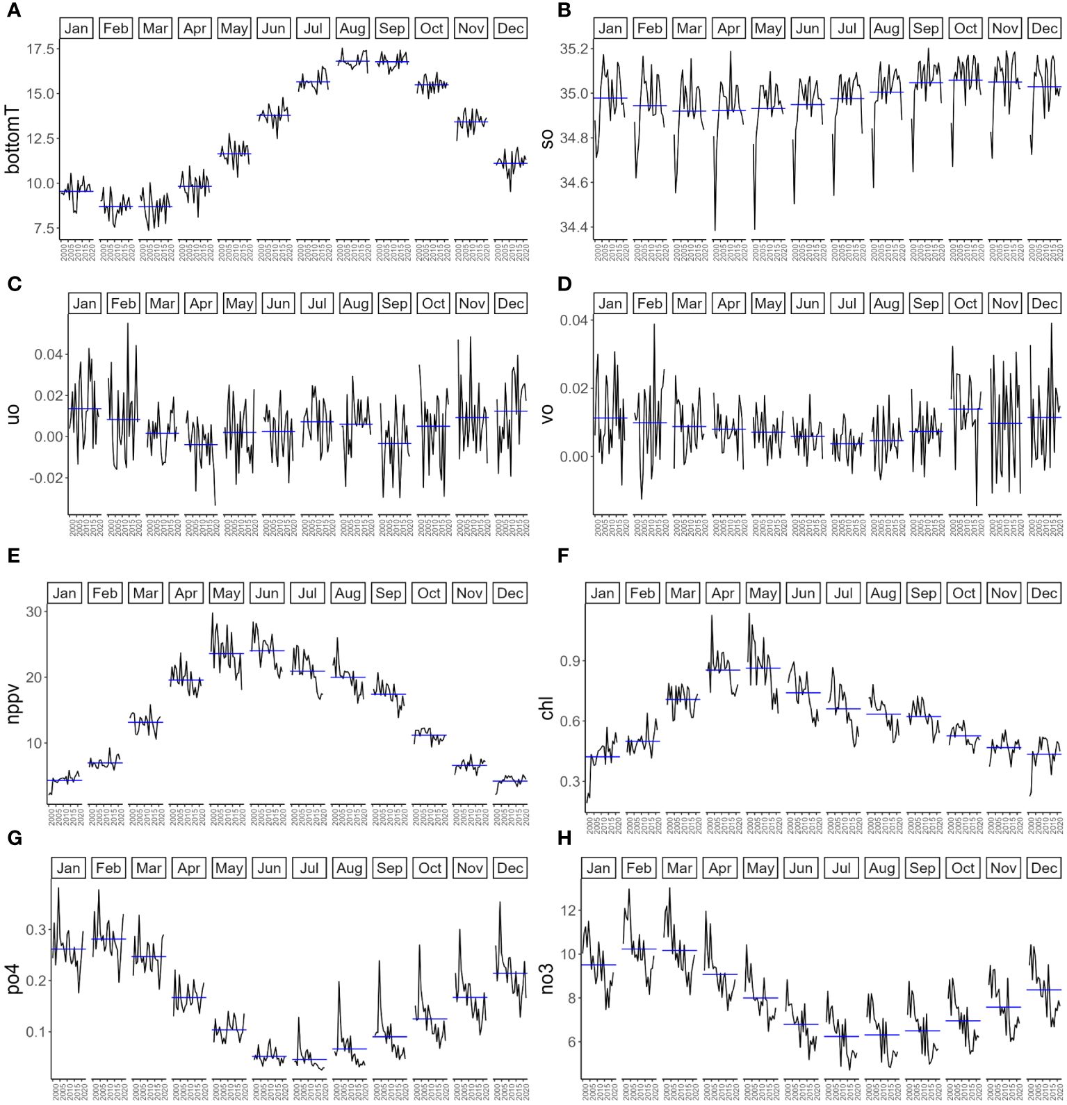
Figure 3 Average per month for each environmental parameter in the English Channel between 2000 and 2021: (A) Bottom temperature (bottomT) in °C; (B) Salinity (so) in PSU; (C) Eastward sea water velocity (uo) in m.s-1; (D) Northward sea water velocity (vo) in m.s-1; (E) Primary production (nppv) in mg.m-3.j-1; (F) Chlorophyll concentration in mg.m-3; (G) Phosphate concentration (po4) in mmol.m-3 and (H) Nitrate concentration (no3) in mmol.m-3. Blue horizontal lines indicate the mean of each month.
Bottom temperature (bottomT), primary production (nppv), chlorophyll concentration (chl), phosphate concentration (po4) and concentration of nitrate (no3) showed important seasonal variations and low interannual variations. Bottom temperature gradually increased from April with an average value of 9.82°C to August with an average value of 16.80°C. From August to March, bottom temperature decreased to a minimum average of 8.68°C in March. Primary production and chlorophyll concentration showed similar seasonal patterns with a gradual increase from February (average values of 4.31 mg.m-3.j-1 for primary production and 0.49 mg.m-3 for chlorophyll concentration) to May-June, with the highest values (average values of 24 mg.m-3.j-1 for primary production in June and 0.86 mg.m-3 for chlorophyll in May) and a gradual decrease from June-July to the lowest values in December-January (average values of 4.20 mg.m-3.j-1 for primary production in December and 0.42 mg.m-3 for chlorophyll in January). Phosphate and nitrate concentration also showed similar seasonal patterns with a gradual increase from August (with an average value of 0.07 mmol.m-3 for phosphate concentration and 6.31 mmol.m-3 for nitrate concentration) to February, which had the highest values (with an average value of 0.28 mmol.m-3 for phosphate concentration and 10.23 mmol.m-3 for nitrate concentration). Salinity showed slight seasonal variations with an increase from April (with an average value of 34.92 PSU) to October, which had the highest values (with an average value of 35.06 PSU). From November to March, salinity decreased to the lowest values (with an average value of 34.92 PSU). In comparison with other environmental variables currents seem to show high interannual variation and low seasonal variation. This sounds logical because currents in the English Channel are mainly tidal currents (not at all seasonal). Besides, we observe averages which are the resulting trend and its anomalies (which most likely depend on wind).
The VIF values used to explore multicollinearity of the variables during the pre-recruitment period (4, 5, 6 and 7 months before the recruitment for each of the two species) showed a high multicollinearity value (VIF>10) for concentration of phosphate and primary production, which were mainly correlated with nitrate and chlorophyll concentrations respectively (Appendix 2 and 3). Therefore, only nitrate and chlorophyll were excluded from the analysis.
3.3 GAM analysis
GAMs were used to fit and predict the effects of environmental variables during the pre-recruitment period (7, 6, 5 or 4 months before recruitment), on recruitment biomass indices in July for L. forbesii (BIJuly) and in November for L. vulgaris (BINovember), and on spatial localization. The spatial and environmental explanatory variables used were bottom temperature (bottomT), salinity (so), eastward current (uo), northward current (vo), phosphate concentration (po4), primary production (nppv) and latitude (lat) x longtude (lon) (i..e incorporating the main effects of both variables plus their interaction).
In total, 8 models were fitted (Table 3).
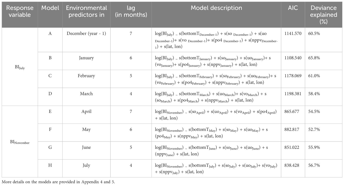
Table 3 Best GAM fitted for each time lag (4, 5, 6 and 7 months before recruitment) for Loligo spp. recruitment biomass indices (in July for L. forbesii and in November for L. vulgaris).
The best model performance for recruitment biomass indices in July occurred in model B with environmental predictors in January (6 month-lag), which has the best AIC: 1108.540. For recruitment biomass indices in November, the best model performance occurred in model H with environmental predictors in July (4 month-lag), which has the best AIC: 838.428. The validity of the models was tested (Appendix 6 and 7). The GAM residuals followed a normal distribution and complied with assumptions about homoscedasticity and independence.
Model B and model H are described in more detail below.
3.4 Model B - Recruitment biomass indices in July – Loligo forbesii
The deviance explained by the explanatory variables included in model B (Table 4) was 65.8% with R2 being 0.64. The most influential factor was the latitude x longitude, with a relative contribution of 33.9%, followed by the bottom temperature in January (bottomTJanuary), the salinity in January (soJanuary) and the primary production in January (nppvJanuary), with the relative contributions being 9.62%, 7.68% and 6.30%.

Table 4 Goodness of fit measures for model B (for the July biomass index) at each stage of the forwards selection process.
Among the environmental factors (Figure 4), bottomTJanuary was the most important influencing factor and was negatively correlated with BIJuly. BIJuly was the highest around 6°C and the lowest between 10 and 12°C. Salinity in January (soJanuary) was the second most important environmental influencing factor. There was no notable trend in BIJuly values within the range of 31 to 34 PSU. However, a negative correlation with BIJuly was observed when soJanuary exceeded 34 PSU. The third was the primary production in January (nppvJanuary) which is negatively correlated with BIJuly: BIJuly was the highest when nppvJanuary approaches zero and the lowest around 8 mg.m-3.j-1. Eastward current in January (uoJanuary) was the 4th most important environmental influencing factor with highest values for BIJuly with an eastward current of 0.2 m.s-1. Phosphate concentration in January (po4January) and the northward current in January (voJanuary) showed the smallest contributions to the model with lowest values of BIJuly when po4January is below 0.4 mmol.m-3 and highest values of BIJuly when voJanuary is negative (maximum around -0.2 m.s-1).
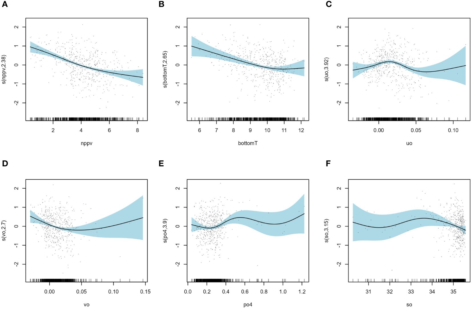
Figure 4 Results of model B: smoothers illustrating the partial effects of environmental variables on the July recruitment biomass index (A) primary production in January (nppvJanuary), (B) bottom temperature in January (bottomTJanuary), (C) eastward current in January (uoJanuary), (D) north current in January (voJanuary), (E) phosphate concentration in January (po4January) and (F) salinity in January (soJanuary).
The effect of latitude x longitude (Figure 5), the most important influencing factor, indicates that BIJuly showed highest values at high latitude between 49.7° and 50.7°N and longitude between -2 and -4°E corresponding to the western part of the English Channel.
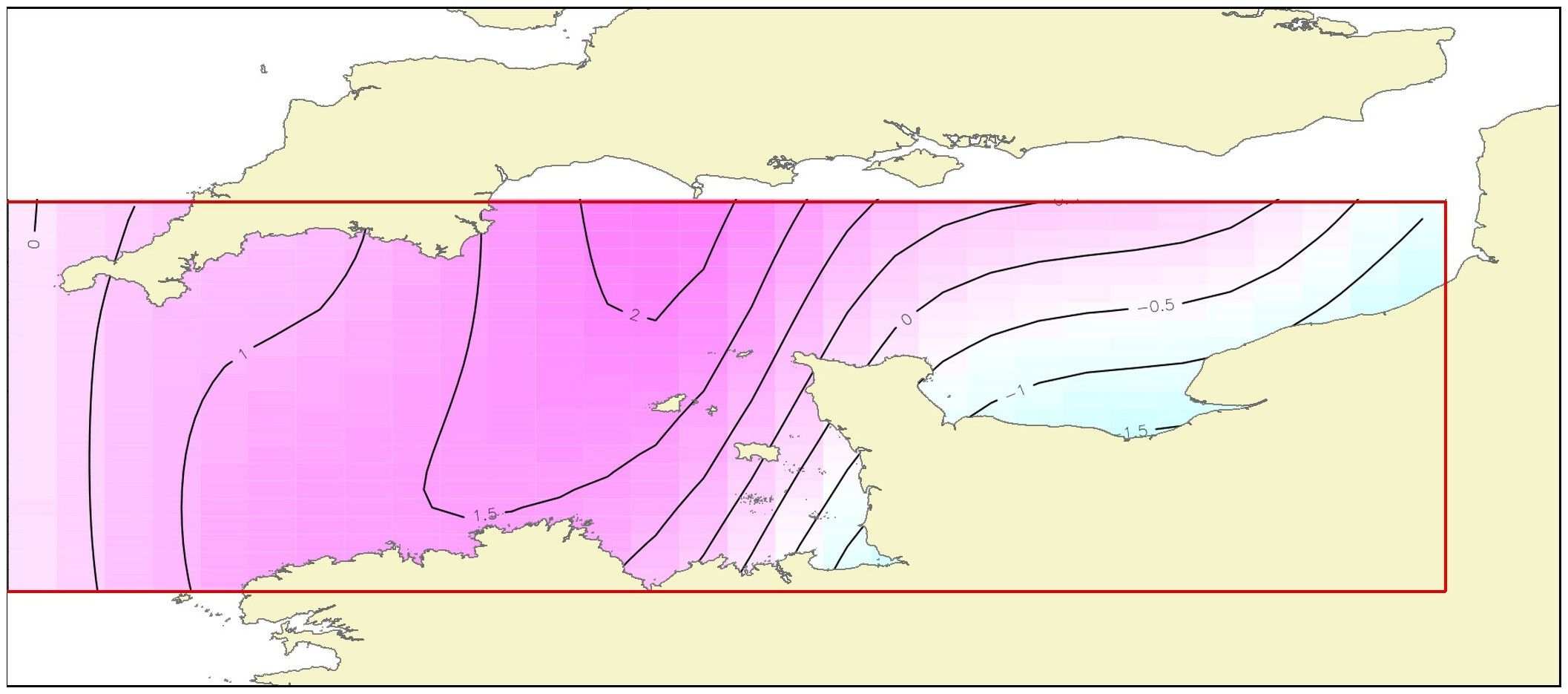
Figure 5 Results of model B: contour plot illustrating the partial effect of latitude and longitude and their interaction on the July recruitment biomass index. The strength and direction of the effect is indicated by the contour labels and shading. The strongest shading indicates the strongest positive effect.
3.5 Model H - Recruitment biomass in November - Loligo vulgaris
Deviance explained by explanatory variables of model H (Table 5) was 56.7% with R2 being 0.55. The latitude x longitude term had the strongest influence, with a relative contribution of 23.1% and the bottom temperature in July (bottomTJuly) with a relative contribution of 20%, followed by the primary production in July (nppvJuly), the salinity in July (soJuly), the eastward current in January (uoJuly) and the northward current in July (voJuly), with the relative contribution being 5.1%, 3.5%, 2.5% and 2.5%.
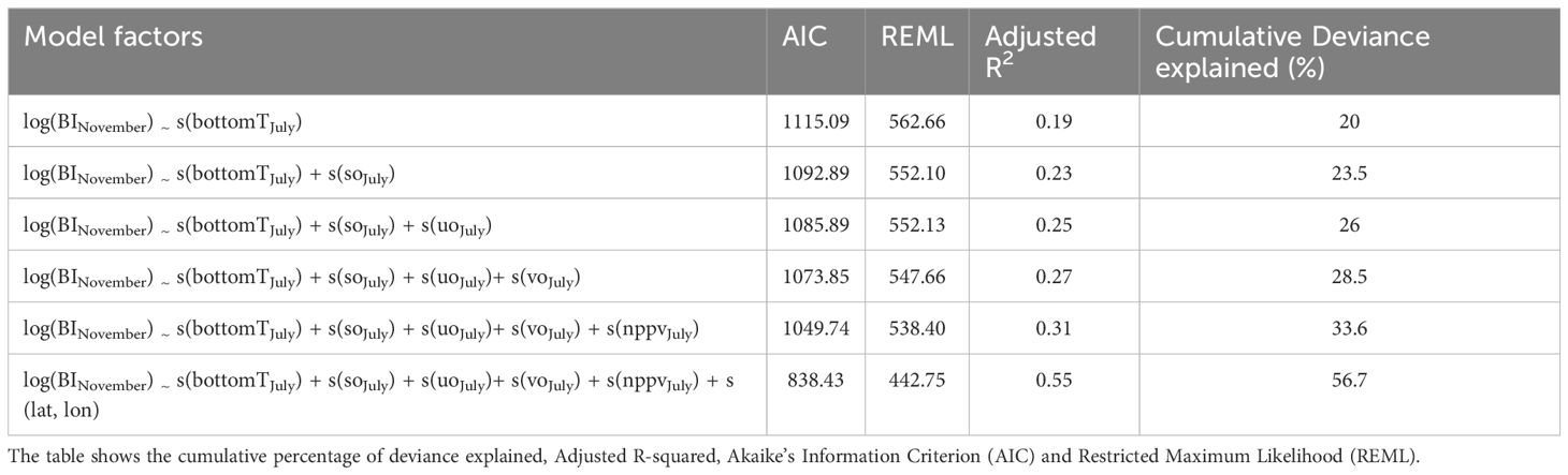
Table 5 Goodness of fit measures for model H (for the November biomass index) at each stage of the forwards selection process.
Among the environmental factors (Figure 6), bottomTJuly was the most important influencing factor and was positively correlated with BINovember between 16 and 20°C. The second most important was the primary production in July (nppvJuly) which is negatively correlated with BINovember: BINovember was the highest when nppvJuly approaches zero and the lowest around 100 mg.m-3.j-1. Salinity in July (soJuly) was the third most important environmental influencing factor and was negatively correlated with BINovember between 30 and 34 PSU and positively correlated between 34 and 35.5 PSU. Eastward current in July (uoJuly) and northward current in January (voJuly) showed the smallest contributions to the model and a small negative correlation with BINovember: highest values of BINovember are found when voJuly and uoJuly are negative (maximum around -0.04 m.s-1 for each factor).
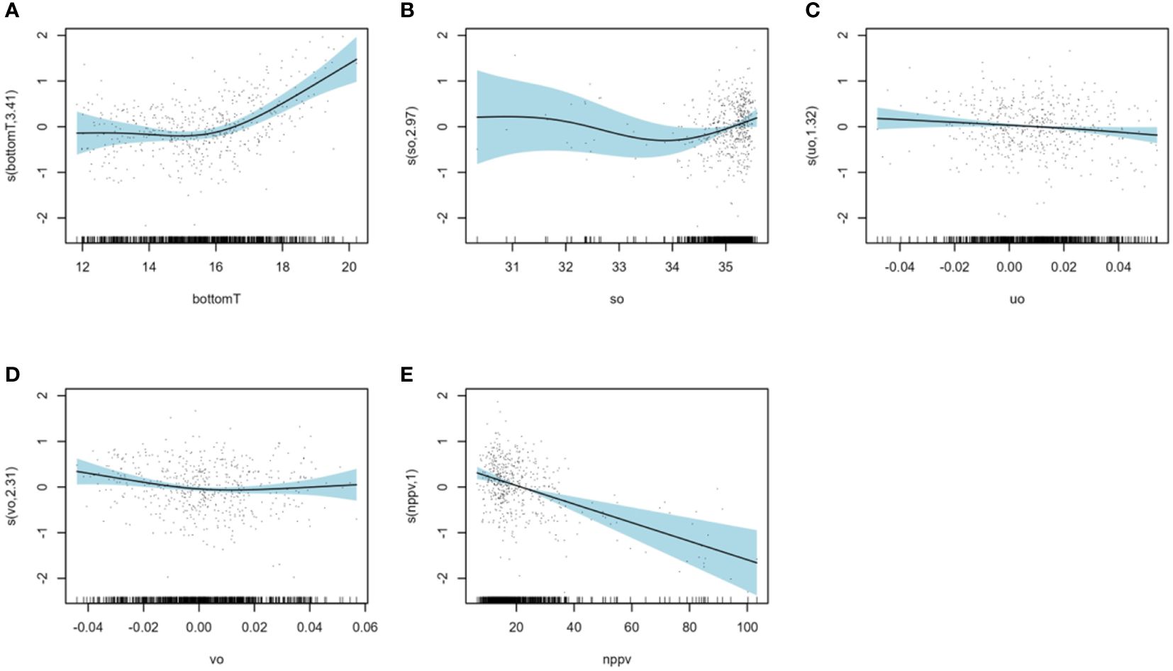
Figure 6 Results of model H: smoothers illustrating the partial effects of environmental variables on the November recruitment biomass index: (A) bottom temperature in July (bottomTJuly), (B) salinity in July (soJuly), (C) eastward current in July (uoJuly), (D) north current in July (voJuly) and (E) primary production in July (nppvJuly).
The effect of latitude x longitude (Figure 7), the most influencing factor, indicates that BINovember showed highest values at high latitude between 49.8° and 50.7°N and longitude between 0 and 1.5°E corresponding to the eastern part of the English Channel.
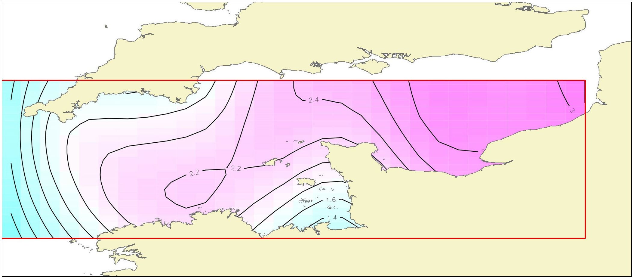
Figure 7 Results of model H: contour plot illustrating the partial effect of latitude and longitude and their interaction on the November recruitment biomass index. The strength and direction of the effect is indicated by the contour labels and shading. The strongest shading indicates the strongest positive effect.
3.6 Predictions of the best models
First, we examined how our models (model B and model H) were able to predict recruitment biomass indices in July and in November over all ICES rectangle of the English Channel (Figure 8). The two models fitted for the 2000–2018 data were tested with the data from the final three years (2019–2021).
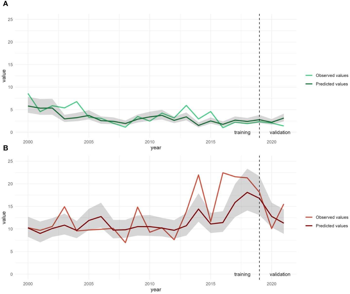
Figure 8 Mean observed and predicted values for recruitment biomass in July (A, in green) and in November (B, in red) over all ICES rectangles in the English Channel. Predictions were obtained from models B and H respectively. The 95% confidence intervals are shown in gray.
For recruitment biomass indices in July, mean predicted values from 2000 to 2018 are very similar with mean observed values and trends suggesting a good fitting of our model. Slight underestimates were noticed in 2003, 2004, 2013, 2014 and 2015. From 2019 to 2021, model B seem to fit quite well except for a small overestimate in 2021. For recruitment biomass indices in November, mean predicted values from 2000 to 2018 are quite similar with mean observed values with similar range and following trends. However, some underestimates were noticed in 2003, 2009, 2014 and from 2016 to 2018 and one overestimate in 2008. From 2019 to 2021, model H seem to fit quite well except for a small underestimate in 2021.
Then, we examined how our models were able to predict recruitment biomass indices in each ICES rectangle of the English Channel from the final three years (2019–2021; Figure 9) that were not included to build the models (2000–2018).
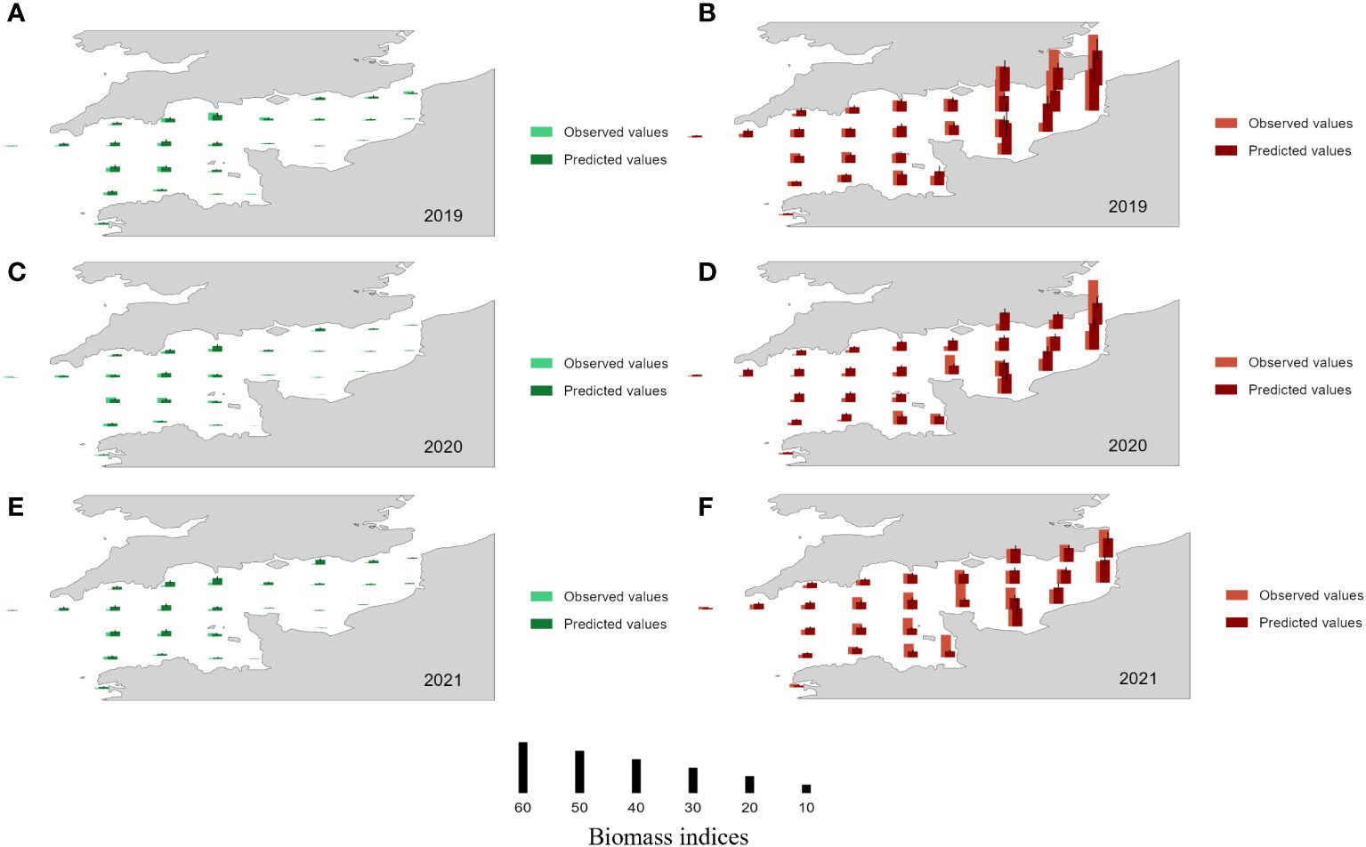
Figure 9 Observed (light color) and predicted values (dark color) for recruitment biomass in each ICES rectangle, in July (left panels, green) and in November (right panels, red). Predictions were obtained by applying models B (July) and H (November) to the subset of data not used to fit the models for 2019 (A, B), 2020 (C, D) and 2021 (E, F). Mean 95% confidence intervals are shown with a black line.
From 2019 to 2021, model B seems to predict well the recruitment biomass indices in July in each ICES rectangle except for a small overestimate in 2021 in all ICES rectangles. Model H seems also to predict quite well the recruitment biomass indices in November in the major part of ICES rectangles. The main discrepancies (between observations and predicted results) occur in the rectangle 30F1 for the three years, in the rectangle 30F0, 29F0 and 29E9 in 2020 and in the rectangle 28E8 in 2021 (underestimates) and in the rectangle 28F0 and 27E9 in 2020 (overestimates).
4 Discussion
Cephalopod populations are known to fluctuate greatly from year to year, probably due to high and variable mortality rates during their planktonic stage as a result of environmental factors (Pierce et al., 2010).
In this study, we investigated the influence of environmental parameters during the pre-recruitment period on biomass indices in July and in November (which most likely correspond to the recruitment of L. forbesii and L. vulgaris, respectively in the English Channel fishery) and on their spatial localization in the English Channel. By understanding how environmental factors affect recruitment, and hence interannual variability, we may be able to predict likely stock size in upcoming seasons prior to recruitment (Arkhipkin et al., 2015).
Before exploring the influence of environment on recruitment, we confirm the consistent seasonal recruitment pattern for both species, as previously proposed by Royer et al. (2002). At least in L. forbesii, it has been suggested that the timing of the life cycle has varied over the years (Pierce et al., 2005) however examination of the time series of monthly data did not reveal the occurrence of such a phenomenon in the English Channel.
To identify the most influential period for recruitment, several months during the pre-recruitment period (4, 5, 6 and 7 months before recruitment) were considered for environmental variables. For L. forbesii recruitment (biomass indices in July), the best model was obtained with environmental predictors in January (6 month-lag). These observations are consistent with Holme’s hypothesis (1974) and Sims et al. (2001) suggesting that L.forbesii juveniles hatched from eggs in the western English Channel in December/January and with the observations of Laptikhovsky et al. (2022), which showed squid paralarvae and juveniles in January/February in the western English Channel. It is the deepest part of the Channel and L. forbesii is known to spawn in deep waters (Pham et al., 2009; Laptikhovsky et al., 2022). For L. vulgaris recruitment (biomass indices in November), the best model was obtained with environmental predictors in July (4 month-lag). Laptikhovsky et al. (2022) observations showed squid paralarvae and juveniles in July/August in the eastern part of the English, which is consistent with the preference of L. vulgaris for spawning in waters shallower than 50 m (Jereb et al., 2015).
The time lag between the period most influencing recruitment and recruitment itself seems to be greater for L. forbesii (6 month-lag) than for L. vulgaris (4 month-lag). This lag difference might be due to the life strategy L. vulgaris, such that it is able to reduce the duration of the vulnerable planktonic phase to increase its survival under warmer conditions (Moreno et al., 2012).
Results of the GAM analyses support this view, since bottom temperature during the pre-recruitment period is the environmental factor with the greatest influence on the L. vulgaris and L. forbesii recruitment with a deviance explained of 20% and 9.62% respectively. Bottom temperature during the pre-recruitment period played a positive role in L. vulgaris recruitment: warmer temperatures may lead to rapid development of paralarvae and juveniles, by shortening the duration of the egg phase and hence increase L. vulgaris recruitment (Moreno et al., 2012). On the contrary, increased bottom temperature during the pre-recruitment period has a negative effect on L. forbesii recruitment. A similar negative effect of temperature was found by Challier et al. (2005) for L. forbesii in the English Channel and for another squid (Doryteuthis gahi) in the Falkland Islands (Agnew et al., 2000). Spawning in L. forbesii takes place deeper waters, usually of under 150 m depth but sometimes at 300–500 m or even 700 m deep (Lordan and Casey, 1999; Salman and Laptikhovsky, 2002) and therefore at lower temperatures. GAM analysis showed highest recruitment when bottom temperature during the pre-recruitment period is around 6°C and the lowest recruitment between 10 and 12°C. This is congruent with the findings of Gowland et al. (2002) indicating that L. forbesii hatching size decreases with increasing temperature.
By changing osmotic pressure, salinity affects the physiological activities of marine organisms (Boeuf and Payan, 2001). GAM analysis indicated a contribution of 7.68% and 3.5% for salinity during the pre-recruitment period respectively for L. forbesii and L. vulgaris recruitment. High salinity during the pre-recruitment period has a negative effect when salinity exceeds 34 PSU for L. forbesii recruitment. On the opposite, L. vulgaris recruitment showed an increasing trend when salinity exceeded 34 PSU. Similar results were found for L. forbesii, with preferred salinity values for spawning animals below 35 PSU in winter in Scotland (Smith et al., 2013). For L. vulgaris, laboratory studies showed that salinity below 34 PSU produces embryonic mortality at early stages of development (Sen, 2004) and Laptikhovsky et al. (2021) have shown egg masses distributed in waters with salinities between 35 and 35.5 PSU.
For both species, primary production during the pre-recruitment period apparently has a negative effect on recruitment, with a contribution of 6.3% for L. forbesii and 5.1% for L.vulgaris. A similar trend has been observed for other cephalopod species such as Doryteuthis opalescens in California coast (Van Noord, 2020) and Octopus cyanea in Tanzania (Chande et al., 2021). In environments characterized by high primary production, the availability of food resources can support a larger number of predators, which in turn can intensify predation pressure on vulnerable cephalopod paralarvae and juveniles (Coll et al., 2008; Puerta et al., 2015).
Eastward and northward currents in the pre-recruitment period showed small contributions to the model for both species recruitment (4.30% and 1.20% for L. forbesii and 2.5% and 2.5% for L. vulgaris) with maximum recruitment for low velocity current in the pre-recruitment period. Late embryonic stages can be prematurely hatched due to high current speeds (Vidal and von Boletzky, 2014).
Under a scenario of global warming, our findings suggest a potential increase in L. vulgaris recruitment corresponding to observed rises in temperature and salinity, as detailed by Oesterwind et al. (2022). L. vulgaris could experience a shorter paralarval stage with a faster growth and maturity at smallest size and younger age, favoring recruitment and the rapid turnover of L. vulgaris populations (Moreno et al., 2012). On the other hand, L. forbesii recruitment should be negatively impacted by climate change with the rising temperature and salinity. This is consistent with observations of fishery landings at the Port-en-Bessin fish market suggesting that the proportion of L. forbesii is decreasing while L. vulgaris is increasing over time in the English Channel (1993-today; Royer, 2002; ICES, 2016 and ICES, 2020) and the finding of Oesterwind et al. (2022) that the distribution range of L. forbesii has declined in the English Channel.
The fact that in both models (B and H) geographic coordinates show the highest contribution to the estimation of biomass indices underlines that in both squid species there is a general spatial pattern of recruitment that is apparently independent of environmental conditions. L. forbesii recruits tend to appear in the Western part of the Channel, an area where the bathymetry ranges from 50 to 100 m (even close to the coast of Devon and Dorset). On the other hand, L. vulgaris recruitment occurs in the Eastern part of the Channel, generally shallower than 50 m. The additional information that environmental variables bring to explaining these distributions suggest that July recruitment tends to be higher in rectangles which underwent severe winter conditions (low temperatures and primary production) whereas November recruits will be likely more important in rectangles in which summer conditions were warm. This can be seen when looking at differences between maps of biomass indices (Appendix 1).
The models explained 65.8% and 56.7% of deviance in recruitment biomass indices of L. forbesii and L. vulgaris respectively and could be useful for predicting biomass indices in upcoming years. Over the last three years of our data (2019–2021), the models forecasts aligned closely with observed trends and values, reinforcing their potential utility for future forecasting. Based on these predictions, at the start of the year (January), it may be possible to estimate biomass indices for July, and similarly, from July, we could predict November biomass using environmental parameters. Such forecasts could inform how and where the fishing season may unfold, enabling the implementation of technical measures to support local and regional fisheries management, and contributing to marine spatial planning. These measures could include setting quotas, extension or shortening fishing periods, modification of the minimum landing size or zone closures to protect recruits (Sobrino et al., 2020).
However, it is important to approach these results with caution. While the models have demonstrated utility, their future performance is not guaranteed, as environmental variations and other factors (such as other anthropogenic impacts or physiological adaptations) might impact their accuracy (Solow, 2002).
Data availability statement
The original contributions presented in the study are included in the article/Supplementary Material. Further inquiries can be directed to the corresponding author.
Author contributions
AM: Conceptualization, Data curation, Formal analysis, Investigation, Methodology, Writing – original draft. EF: Resources, Writing – review & editing. GP: Methodology, Supervision, Validation, Writing – review & editing. J-PR: Conceptualization, Funding acquisition, Methodology, Resources, Supervision, Validation, Writing – review & editing.
Funding
The author(s) declare financial support was received for the research, authorship, and/or publication of this article. Funding support for this work has been provided by France Filière Pêche (FFP) and by the Conseil Régional de Basse Normandie. We would like to thank the Système d’Information Halieutique (SIH) of the Ifremer for providing us with French commercial landings and the French Direction des Pêches Maritimes et de l’Aquaculture (DPMA) for granting permission for using commercial data.
Conflict of interest
The authors declare that the research was conducted in the absence of any commercial or financial relationships that could be construed as a potential conflict of interest.
Publisher’s note
All claims expressed in this article are solely those of the authors and do not necessarily represent those of their affiliated organizations, or those of the publisher, the editors and the reviewers. Any product that may be evaluated in this article, or claim that may be made by its manufacturer, is not guaranteed or endorsed by the publisher.
Supplementary material
The Supplementary Material for this article can be found online at: https://www.frontiersin.org/articles/10.3389/fmars.2024.1433071/full#supplementary-material
References
Agnew D. J., Hill S., Beddington J. R. (2000). Predicting the recruitment strength of an annual squid stock: Loligo gahi around the Falkland Islands. Can. J. Fish. Aquat. Sci. 57, 2479–2487. doi: 10.1139/f00-240
Araújo M. B., Anderson R. P., Márcia Barbosa A., Beale C. M., Dormann C. F., Early R., et al. (2019). Standards for distribution models in biodiversity assessments. Sci. Adv. 5, eaat4858. doi: 10.1126/sciadv.aat4858
Arkhipkin A. I., Rodhouse P. G., Pierce G. J., Sauer W., Sakai M., Allcock L., et al. (2015). World squid fisheries. Rev. Fish. Sci. Aquac. 23 (2), 92–252. doi: 10.1080/23308249.2015.1026226
Arkhipkin A. I., Hendrickson L. C., Payá I., Pierce G. J., Roa-Ureta R. H., Robin J. P., et al. (2021). Stock assessment and management of cephalopods: advances and challenges for short-lived fishery resources. ICES J. Mar. Sci. 78, 714–730. doi: 10.1093/icesjms/fsaa038
Bloor I. S., Attrill M. J., Jackson E. L. (2013). A review of the factors influencing spawning, early life stage survival and recruitment variability in the common cuttlefish (Sepia officinalis). Adv. Mar. Biol. 65, 1–65. doi: 10.1016/B978-0-12-410498-3.00001-X
Boeuf G., Payan P. (2001). How should salinity influence fish growth? Comp. Biochem. Physio l- C Toxicology and Pharmacology 130 (4), 411–423. doi: 10.1016/S1532-0456(01)00268-X
Boletzky S. V. (1979). Observations on the early post-embryonic development of Loligo vulgaris (Mollusca, Cephalopoda). Rapport de la Commission Internationale Pour la Mer Méditerranée, 25/26(10). 155–158.
Boyle P. (2002). Cephalopod biomass and production: an introduction to the symposium. Bull. Mar. Sci. 71 (1), 13–16.
Brodie S. J., Thorson J. T., Carroll G., Hazen E. L., Bograd S., Haltuch M. A., et al. (2020). Trade-offs in covariate selection for species distribution models: a methodological comparison. Ecography 43, 11–24. doi: 10.1111/ecog.04707
Bruggeman J., Jacobs Z. L., Popova E., Sauer W. H., Gornall J. M., Brewin R. J., et al. (2022). The paralarval stage as key to predicting squid catch: Hints from a process-based model. Deep Sea Res. Part II: Top. Stud. Oceanogr. 202, 105123. doi: 10.1016/j.dsr2.2022.105123
Caddy J. F. (1983). “The cephalopods: factors relevant to their population dynamics and to the assessment and management of stocks,” in Advances in assessment of world cephalopod resources, vol. 231. (FAO Fish. Tech. Pap., Rome), 416–457.
Challier L., Royer J., Pierce G. J., Bailey N., Roel B., Robin J.-P. (2005). Environmental and stock effects on recruitment variability in the English Channel squid Loligo Forbesi. Aquat. Living Resour. 18, 35. doi: 10.1051/alr:2005024
Chande M. A., Mgaya Y. D., Benno L. B., Limbu S. M. (2021). The influence of environmental variables on the abundance and temporal distribution of Octopus cyanea around Mafia Island, Tanzania. Fisheries Res. 241, 105991. doi: 10.1016/j.fishres.2021.105991
Chatterjee S., Hadi A. S., Price B. (2000). Regression analysis by example (New York, New York, USA: John Wiley and Sons).
Coll M., Palomera I., Tudela S., Dowd M. (2008). Food-web dynamics in the South Catalan Sea ecosystem (NW Mediterranean) for 1978–2003. Ecol. Model. 217, 95–116. doi: 10.1016/j.ecolmodel.2008.06.013
Craig S. (2001). Environmental conditions and yolk biochemistry: factors influencing embryonic development in the squid Loligo forbesi (Cephalopoda: Loliginidae) Steenstrup 1856 (United Kingdom: University of Aberdeen).
Dawe E. G., Hendrickson L. C., Colbourne E. B., Drinkwater K. F., Showell M. A. (2007). Ocean climate effects on the relative abundance of short-finned (Illex illecebrosus) and long-finned (Loligo pealeii) squid in the northwest Atlantic Ocean. Fisheries Oceanogr. 16, 303–316.3–360. doi: 10.1111/j.1365-2419.2007.00431.x
Doubleday Z. A., Prowse T. A., Arkhipkin A., Pierce G. J., Semmens J., Steer M., et al. (2016). Global proliferation of cephalopods. Curr. Biol. 26, R406–R407. doi: 10.1016/j.cub.2016.04.002
Fogarty M. J. (1989). “Forecasting yield and abundance of exploited invertebrates,” in Marine Invertebrate Fisheries: Their Assessment and Management (New York: John Wiley and Sons), 701–724. Available at: https://archive.org/details/marineinvertebra0000unse_h2m8.
Fuiman L. A. (2002). Special consideration on fish eggs and larvae. In Fuiman L., Werner R. (Eds.) Fishery science: the unique contributions of early life stages. Blackwell Sciences. pp. 1–32.
Gowland F. C., Boyle P. R., Noble L. R. (2002). Morphological variation provides a method of estimating thermal niche in hatchlings of the squid Loligo forbesi (Mollusca: Cephalopoda). J. Zool. 258, 505–513. doi: 10.1017/S0952836902001668
Guerra Á., Allcock L., Pereira J. (2010). Cephalopod life history, ecology and fisheries: An introduction. Fisheries Res. 106, 117–124. doi: 10.1016/j.fishres.2010.09.002
Guerra A., Rocha F. (1994). The life history of Loligo vulgaris and Loligo forbesi (Cephalopoda: Loliginidae) in Galician waters (NW Spain). Fisheries Res. 21, 43–69. doi: 10.1016/0165-7836(94)90095-7
Han H., Yang C., Zhang H., Fang Z., Jiang B., Su B., et al. (2022). Environment variables affect CPUE and spatial distribution of fishing grounds on the light falling gear fishery in the northwest Indian Ocean at different time scales. Front. Mar. Sci. 9, 939334. doi: 10.3389/fmars.2022.939334
Holme N. A. (1974). The biology of Loligo forbesi Steenstrup (Mollusca: Cephalopoda) in the Plymouth area. J. Mar. Biol. Assoc. United Kingdom 54, 481–503. doi: 10.1017/S0025315400058665
ICES (2016). Interim report of the working group on cephalopod fisheries and life history (WGCEPH), 8–11 June 2015, Tenerife, Spain. ICES CM 2015/SSGEPD:02, 127pp.
ICES (2020). Working Group on Cephalopod Fisheries and Life History (WGCEPH; outputs from 2019 meeting). ICES Sci. Rep. 2, 121. doi: 10.17895/ices.pub.6032
Jereb P., Allcock L. A., Lefkaditou E., Piatkowski U., Hastie L. C., Pierce G. J. (2015). Cephalopod biology and fisheries in Europe: II. Species Accounts. Co-operative Research Report No 325. (Copenhagen: International Council for the Exploration of the Sea) 360pp.
Kim J. J., Stockhausen W., Kim S., Cho Y. K., Seo G. H., Lee J. S. (2015). Understanding interannual variability in the distribution of, and transport processes affecting, the early life stages of Todarodes pacificus using behavioral-hydrodynamic modeling approaches. Prog. Oceanogr. 138, 571–583. doi: 10.1016/j.pocean.2015.04.003
Laptikhovsky V., Allcock A. L., Barnwall L., Barrett C., Cooke G., Drerup C., et al. (2022). Spatial and temporal variability of spawning and nursery grounds of Loligo forbesii and Loligo vulgaris squids in ecoregions of Celtic Seas and Greater North Sea. ICES J. Mar. Sci. 79, 1918–1930. doi: 10.1093/icesjms/fsac128
Laptikhovsky V., Cooke G., Barrett C., Lozach S., MacLeod E., Oesterwind D., et al. (2021). Identification of benthic egg masses and spawning grounds in commercial squid in the English Channel and Celtic Sea: Loligo vulgaris vs L. forbesii. Fisheries Res. 241, 106004. doi: 10.1016/j.fishres.2021.106004
Legendre P. (1993). Spatial autocorrelation: trouble or new paradigm? Ecology 74, 1659–1673. doi: 10.2307/1939924
Lehmann A., Overton J. M., Leathwick J. R. (2002). GRASP: generalized regression analysis and spatial prediction. EcolModel 157, 189–207. doi: 10.1016/S0304-3800(02)00195-3
Lordan C., Casey J. (1999). The first evidence of offshore spawning in the squid species Loligo forbesi. J. Mar. Biol. Assoc. United Kingdom 79, 379–381. doi: 10.1017/S0025315498000484
Mangold-Wirz K. (1963). Biologie des Céphalopodes benthiques et nectoniques de la Mer Catalane (Vie et Milieu) Suppl. 13, 285. Available at: https://hal.science/hal-03330666/.
Marcout A., Foucher E., Pierce G., Robin J. P. (2024). Derivation of a standardized index to explore spatial, seasonal and between-year variation of squid (loligo spp.) abundance in the english channel. doi: 10.2139/ssrn.4791845
Moreno A., Pereira J., Arvanitidis C., Robin J. P., Koutsoubas D., Perales-Raya C., et al. (2002). Biological variation of Loligo vulgaris (Cephalopoda: Loliginidae) in the eastern Atlantic and Mediterranean. Bull. Mar. Sci. 71, 515–534.
Moreno A., Pierce G. J., Azevedo M., Pereira J., Santos A. M. P. (2012). The effect of temperature on growth of early life stages of the common squid Loligo vulgaris. J. Mar. Biol. Assoc. 92, 1619–1628. doi: 10.1017/S0025315411002141
Moustahfid H., Hendrickson L. C., Arkhipkin A., Pierce G. J., Gangopadhyay A., Kidokoro H., et al. (2021). Ecological-fishery forecasting of squid stock dynamics under climate variability and change: review, challenges, and recommendations. Rev. Fisheries Sci. Aquaculture 29, 682–705. doi: 10.1080/23308249.2020.1864720
Murase H., Nagashima H., Yonezaki S., Matsukura R., Kitakado T. (2009). Application of a generalized additive model (GAM) to reveal relationships between environmental factors and distributions of pelagic fish and krill: a case study in Sendai Bay, Japan. ICES J. Mar. Sci. 66, 1417–1424. doi: 10.1093/icesjms/fsp105
Neter J., Kutner M. H., Nachtsheim C. J., Wasserman W. (1996). Applied linear statistical models (Chicago,Illinois, USA: Irwin).
Oesterwind D., Barrett C. J., Sell A. F., Núñez-Riboni I., Kloppmann M., Piatkowski U., et al. (2022). Climate change-related changes in cephalopod biodiversity on the North East Atlantic Shelf. Biodiversity Conserv. 31, 1491–1518. doi: 10.1007/s10531-022-02403-y
Pham C. K., Carreira G. P., Porteiro F. M., Gonçalves J. M., Cardigos F., Martins H. R. (2009). First description of spawning in a deep water loliginid squid, Loligo forbesi (Cephalopoda: Myopsida). J. Mar. Biol. Assoc. United Kingdom 89, 171–177. doi: 10.1017/S0025315408002415
Pierce G. J., Allcock L., Bruno I., Bustamante P., Gonzalez A., Guerra Á., et al. (2010). Cephalopod biology and fisheries in Europe. Co-operative Research Report 303. (International Council for the Exploration of the Sea) 175 pp.
Pierce G. J., Bailey N., Stratoudakis Y., Newton A. (1998). Distribution and abundance of the fished population of Loligo forbesi in Scottish waters: analysis of research cruise data. ICES J. Mar. Sci. 55, 14–33. doi: 10.1006/jmsc.1997.0257
Pierce G. J., Boyle P. R. (2003). Empirical modelling of interannual trends in abundance of squid (Loligo forbesi) in Scottish waters. Fish. Res. 59 (3), 305–326.
Pierce G. J., Boyle P. R., Hastie L. C., Shanks A. M. (1994). Distribution and abundance of the fished population of Loligo forbesi in UK waters: analysis of fishery data. Fisheries Res. 21, 193–216. doi: 10.1016/0165-7836(94)90104-X
Pierce G. J., Guerra A. (1994). Stock assessment methods used for cephalopod fisheries. Fisheries Res. 21, 255–285. doi: 10.1016/0165-7836(94)90108-2
Pierce G. J., Valavanis V. D., Guerra A., Jereb P., Orsi-Relini L., Bellido J. M., et al. (2008). A review of cephalopod–environment interactions in European Seas. Hydrobiologia 612, 49–70. doi: 10.1007/s10750-008-9489-7
Pierce G. J., Zuur A. F., Smith J. M., Santos M. B., Bailey N., Chen C. S., et al. (2005). Interannual variation in life-cycle characteristics of the veined squid (Loligo forbesi) in Scottish (UK) waters. Aquat. Living Resour 18 (4), 327–340.
Puerta P., Hunsicker M. E., Quetglas A., Álvarez-Berastegui D., Esteban A., González M., et al. (2015). Spatially explicit modeling reveals cephalopod distributions match contrasting trophic pathways in the western Mediterranean Sea. PloS One 10, e0133439. doi: 10.1371/journal.pone.0133439
R Development Core Team (2023). R: A language and environment for statistical computing (Vienna, Austria: R Foundation for Statistical Computing). Available at: https://www.R-project.org.
Roa-Ureta R., Arkhipkin A. I. (2007). Short-term stock assessment of Loligo gahi at the Falkland Islands: sequential use of stochastic biomass projection and stock depletion models. ICES J. Mar. Sci. 64 (1), 3–17.
Robin J. P., Boucaud-Camou E. (1995). Squid catch composition in the English Channel bottom trawl fishery: proportion of Loligo forbesi and Loligo vulgaris in the landings and length-frequencies of both species during the 1993–1994 period. ICES CM 1995/K, Vol. 36, 12pp.r.
Rodhouse P. G., Pierce G. J., Nichols O. C., Sauer W. H., Arkhipkin A. I., Laptikhovsky V. V., et al. (2014). Environmental effects on cephalopod population dynamics: implications for management of fisheries. Adv. Mar. Biol. 67, 99–233. doi: 10.1016/B978-0-12-800287-2.00002-0
Royer J., Périès P., Robin J. P. (2002). Stock assessments of english channel loliginid squids: updated depletion methods and new analytical methods. ICES J. Mar. Sci. 59 (3), 445–457.
Salman A., Laptikhovsky V. (2002). First occurrence of egg masses of Loligo forbesi (Cephalopoda: Loliginidae) in deep waters of the Aegean Sea. J. Mar. Biol. Assoc. United Kingdom 82, 925–926. doi: 10.1017/S0025315402006392
Segawa S., Yang W. T., Marthy H. J., Hanlon R. T. (1988). Illustrated embryonic stages of the eastern Atlantic squid Loligo forbesi. Veliger 30, 230–243.
Sen H. (2004). A preliminary study on the effects of salinity on egg development of European squid (Loligo vulgaris Lamarck, 1798). Isr. J. Aquacult.- Bamid. 56, 93–99. doi: 10.46989/001c.20368
Sims D. W., Genner M. J., Southward A. J., Hawkins S. J. (2001). Timing of squid migration refects North Atlantic climate variability. Proc. R Soc. Lond B Biol. Sci. 268, 2607–2611. doi: 10.1098/rspb.2001.1847
Smith J. M., Macleod C. D., Valavanis V., Hastie L., Valinassab T., Bailey N., et al. (2013). Habitat and distribution of post-recruit life stages of the squid Loligo forbesii. Deep Sea Res. Part II: Topical Stud. Oceanogr. 95, 145–159. doi: 10.1016/j.dsr2.2013.03.039
Sobrino I., Rueda L., Tugores M. P., Burgos C., Cojan M., Pierce G. J. (2020). Abundance prediction and influence of environmental parameters in the abundance of Octopus (Octopus vulgaris Cuvier 1797) in the Gulf of Cadiz. Fisheries Res. 221, 105382. doi: 10.1016/j.fishres.2019.105382
Solow A. R. (2002). Fisheries recruitment and the North Atlantic oscillation. Fisheries Res. 54, 295–297. doi: 10.1016/S0165-7836(00)00308-8
Suca J. J., Santora J. A., Field J. C., Curtis K. A., Muhling B. A., Cimino M. A., et al. (2022). Temperature and upwelling dynamics drive market squid (Doryteuthis opalescens) distribution and abundance in the California Current. ICES J. Mar. Sci. 79, 2489–2509. doi: 10.1093/icesjms/fsac186
Thorson J. T. (2019). Guidance for decisions using the Vector Autoregressive Spatio-Temporal (VAST) package in stock, ecosystem, habitat and climate assessments. Fish. Res. 210, 143–161. doi: 10.1016/j.fishres.2018.10.013
Van Noord J. E. (2020). Dynamic spawning patterns in the California market squid (Doryteuthis opalescens) inferred through paralarval observation in the Southern California Bight 2012–2019. Mar. Ecol. 41, e12598. doi: 10.1111/maec.12598
Vayghan A. H., Ray A., Mondal S., Lee M. A. (2024). Modeling of swordtip squid (Uroteuthis edulis) monthly habitat preference using remote sensing environmental data and climate indices. Front. Mar. Sci. 11, 1329254. doi: 10.3389/fmars.2024.1329254
Vidal E. A., von Boletzky S. (2014). “Loligo vulgaris and Doryteuthis opalescens,” in Cephalopod culture, 271–313.
Villanueva R., Arkhipkin A., Jereb P., Lefkaditou E., Lipinski M. R., Perales-Raya C., et al. (2003). Embryonic life of the loliginid squid Loligo vulgaris: comparison between statoliths of Atlantic and Mediterranean populations. Mar. Ecol. Prog. Ser. 253, 197–208.
Keywords: squid, recruitment, English Channel, forecasting, environment, loligo forbesii, loligo vulgaris
Citation: Marcout A, Foucher E, Pierce GJ and Robin J-P (2024) Impact of environmental conditions on English Channel long-finned squid (Loligo spp.) recruitment strength and spatial location. Front. Mar. Sci. 11:1433071. doi: 10.3389/fmars.2024.1433071
Received: 15 May 2024; Accepted: 01 July 2024;
Published: 13 August 2024.
Edited by:
Bernardo Patti, National Research Council (CNR), ItalyReviewed by:
Sergio VitaleGermana Garofalo, National Research Council (CNR), Italy
Stylianos (stelios) Somarakis, Hellenic Center for Marine Research, Greece
Copyright © 2024 Marcout, Foucher, Pierce and Robin. This is an open-access article distributed under the terms of the Creative Commons Attribution License (CC BY). The use, distribution or reproduction in other forums is permitted, provided the original author(s) and the copyright owner(s) are credited and that the original publication in this journal is cited, in accordance with accepted academic practice. No use, distribution or reproduction is permitted which does not comply with these terms.
*Correspondence: Anna Marcout, YW5uYS5tYXJjb3V0QHVuaWNhZW4uZnI=