Research on seamount substrate classification method based on machine learning

The western Pacific seamount area is abundant in both biological and mineral resources, making it a crucial location for international investigation of regional seabed resources. An essential stage in comprehending and advancing seamounts is gaining knowledge about the distribution characteristics and laws governing the seabed substrate. Deep-sea geological sampling is challenging because of the intricate nature of the deep-sea environment, resulting in increased difficulty in identifying and evaluating substrates. This study addresses the aforementioned issues by utilizing in-situ video footage obtained from the “Jiaolong” manned deep submersible and shipborne deep-water multibeam data. This data is used as a foundation for constructing a Western Pacific seamount areas substrate classification point set. Additionally, the paper introduces the mRMR-XGBoost substrate classification model. Substrate categorization in deep sea and mountainous regions has been successfully accomplished, yielding a classification accuracy of 92.5%. The classification experiments and box sampling results demonstrate that the mRMR-XGBoost substrate classification model proposed in this paper can efficiently use acoustic and optical data to accurately divide the substrate types in seamount areas, with better classification accuracy, when compared with commonly used machine learning models. It has a significant application value and the best classification effect on the two types of substrates: nodules and gravel substrates.

1 Introduction

Seamounts, also known as seabed mountains, usually refer to seabed uplifts that are distributed in the deep sea below sea level and are greater than 1000m in height. They are morphologically divided into flat-topped seamounts and pointed-topped seamounts (Gan et al., 2021). Seamounts not only contain rich polymetallic mineral resources, but also rich biological resources, and are a typical ecosystem. The distribution of organisms on seamounts varies vertically, forming a rich variety of habitat types. Its complex topographical and geological features provide a unique habitat environment for marine organisms (Mayer et al., 2018; Victorero et al., 2018). Seamount areas have a variety of bottom types, and the distribution of seabed substrate has always been an important topic in marine science research (Zhu et al., 2022). The distribution characteristics of seabed substrates and geomorphic characteristics can reflect the distribution of seafloor tectonic activities and seafloor evolution information to a certain extent, and are of great significance to the study of seafloor sedimentation processes and biodiversity protection, among other areas (Zhu et al., 2022).

At present, the main means of understanding the seabed environment are station sampling using equipment such as television grabs, gravity sampling and seabed drilling rigs, and seabed line observation using seabed camera towed bodies and video systems carried by manned submersibles. However, due to the point and line operation mode, the above methods are not suitable for broad-scale surveys of the seabed and cannot obtain bottom data for the entire seamount area. The proliferation of ocean detection technology, such as shipborne deep-water multi-beams and manned submersibles, has led to a significant surge in the volume of deep-sea data. Consequently, this has facilitated the comprehensive examination of the substrate properties of seamounts. A Multibeam Echo Sounder (MBES) is an acoustic instrument capable of performing comprehensive seabed mapping. The device is capable of gathering water depth measurements and seabed backscatter intensity data concurrently, allowing for the acquisition of both seabed topography and the distribution of seabed sediments (Chunhui et al., 2015). Currently, much research has been conducted by researchers both domestically and internationally to elucidate the physical and chemical characteristics, spatial arrangement, and other relevant aspects of the seabed. The two primary techniques for substrate detection that are frequently employed are direct sampling and indirect detection (Wang et al., 2021). Direct sampling is widely recognized as the predominant method for acquiring on-site samples. Various sample forms and methods exist based on the characteristics of the substrate. The typical techniques are listed in Table 1 (Wang et al., 2021). Direct sampling involves the utilization of large-scale devices to collect substrate samples directly at the site for in-situ examination. However, this method is associated with high costs, inefficiency, and the need for substantial human and material resources (Wang et al., 2021). One notable benefit is the ability to acquire particle size data in a manner that is both intuitive and precise (Wang et al., 2021). Seafloor optical measurement and acoustic measurement are the primary indirect detection technologies that address the limitations of traditional bottom survey methods, such as limited coverage and low efficiency. Nevertheless, optical measurement is subject to several constraints, including limited detection range and the requirement for diving (Sun et al., 2021). Sound waves has several advantageous characteristics, including their ability to propagate over vast distances and penetrate deep into ocean. Additionally, the backscatter vary depending on the specific seabed substrates. Hence, the utilization of acoustic properties for substrate identification has consistently been a prominent area of investigation within academic circles (Gaida et al., 2020; Yan et al., 2020).

Table 1

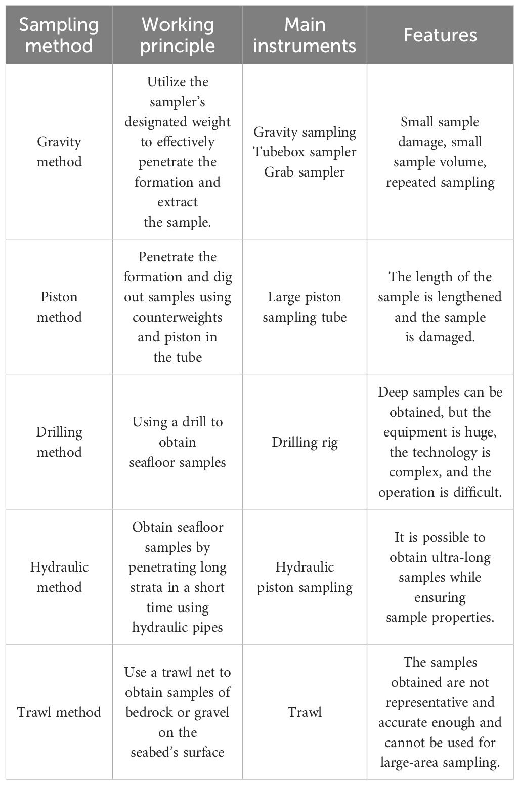
Table 1 Common substrate sampling methods.

The origins of substrate classification study may be traced back to the 1960s, with a primary emphasis on investigating the acoustic characteristics of undersea substrates and extracting elements related to submarine echoes. In 1956, Biot conducted a study on the correlation between phase velocity and group velocity, which varies with frequency and attenuation factor. He developed an acoustic parameter model for inverting sediments on the bottom surface (Biot, 2005). In 1995, Michalopoulou utilized statistical classifiers to classify the state of the seabed. Based on backscatter, a data set was created and the classifier was effectively used to classify North Pacific seamounts (Michalopoulou et al., 1995). Herzfeld and Higginson (1996) proposed a geostatistical approach for the automated classification of seafloors. This method incorporates several criteria for differentiation, such as the spatial arrangement and orientation of deep-sea seamounts, as well as other relevant metrics that capture the intricate nature of seamounts (Herzfeld and Higginson, 1996). The automated seabed classification approach based on backscatter data was developed by Müller in 1997. The Gray-Level Co-occurrence Matrix (GLCM) was employed to extract texture features, followed by the construction of a neural network including 18 identified features. The accuracy of the classification achieved a level of 80% or above (Müller et al., 1997). In 2007, Rooper used a classification tree to establish the relationship between optical data and acoustic data, and determined that reflectivity and seabed roughness were important parameters for seabed classification (Rooper and Zimmermann, 2007). In 2012, Fakiris used unsupervised classification methods to compare the corrected backscatter data with the uncorrected data, clarifying the importance of acoustic backscatter correction for texture analysis (Fakiris et al., 2012).

The utilization of machine learning techniques for substrate categorization has been increasingly prevalent among academics due to the proliferation of broad-scale data. Typical studies include, in 2015, Alevizos tested the ability of Bayesian classifiers to distinguish fine-grained sediments based on high-resolution multibeam data, demonstrating the effectiveness of Bayesian classification techniques (Alevizos et al., 2015). In 2018, Porskamp used a hierarchical classification method to classify tow videos, combined MBES bathymetry data, backscatter, and tow video data to establish a data set, and used a random forest algorithm to achieve habitat mapping from multiple scales (Porskamp et al., 2018). In the year 2020, Rende conducted a study wherein optical and acoustic data were processed using Object Based Image Analysis (OBIA) processing technology. Various multi-scale mapping technologies were employed for data combination, and the reliability of combining acoustic and optical data for high-resolution mapping was demonstrated through testing research involving the KNN, random forest algorithm, and decision tree classifier algorithm (Rende et al., 2020). Ji Xue et al. conducted a study on post-processing methods for multi-beam data. They developed a set of backscatter intensity correction models and developed an optimal random forest seabed automatic classification model. The authors provided empirical evidence to validate the effectiveness of this approach (Ji et al., 2020). Pillay et al. constructed a data set based on multi-beam bathymetry, backscatter and side-scan sonar data, conducted a comparative analysis of decision tree, random forest and K-means clustering algorithms, and drew a benthic habitat map. They believed that the K-means classification algorithm was the easiest and pointed out that underwater videos and underwater samples could be used to verify and explain the classification model in future studies (Pillay et al., 2020). The association between backscatter data obtained from deep water multi-beams and the presence of crusts and nodules in seamounts was established by Yang. Additionally, a quantitative analysis was conducted to examine the distribution of minerals in these seamounts locations (Yang et al., 2020). Zhu and colleagues introduced a classification model for seabed substrate in 2021. This model utilizes a multi-beam and multi-feature deep neural network (DNN) with varying weights. The weights of different characteristics are distributed in a reasonable manner, and the multi-beam features are merged to achieve seabed substrate classification (Zhu et al., 2021). In the year 2022, Tang conducted an examination of diverse errors occurring in the deep-sea environment. The researcher employed both unsupervised and supervised classification techniques to carry out substrate classification research on the Southwest Indian Ocean Ridge. Additionally, genetic algorithms (GA) were utilized to conduct support vector machine (SVM) analysis. The optimum that corresponds to (Tang et al., 2022). Mbani et al. introduced an automated process for classifying seabed substrate s that addresses the issue of classification deviation resulting from differences in resolution and imbalanced categories. This workflow enables automatic classification of seabed substrates with minimal manual annotations (Mbani et al., 2022, Mbani et al., 2023). Jackett et al. manually annotated more than 7,000 seafloor images, used these images to train a convolutional neural network, and used transfer learning, model hyperparameter optimization and other techniques to improve the classification model to a certain extent, with a classification accuracy of 98.19% (Jackett et al., 2023).

In conclusion, following extensive research spanning several decades, scholars have made significant advancements in the methodology for substrate classification. The acquisition of deep-sea multi-beam data poses greater challenges compared to shallow-water multi-beam data due to the intricate nature of the deep-sea environment. Consequently, the acquisition of deep-sea multi-beam data necessitates the use of specialized equipment and data processing techniques. Furthermore, the scarcity of sample labels in marine environments poses challenges in the integration of acoustic and visual data. Consequently, there is a scarcity of research on the attributes of sediments found in deep-sea seamounts. This study deeply mined the in-situ video and ship-borne deep-water multi-beam data collected by the “Jiaolong” manned submersible, obtained a variety of characteristic factors that characterize the characteristics of the bottom, and maximized the use of valuable deep-sea data. A feature matching algorithm was used to establish the connection between acoustic features and optical data, and a substrate classification point set for the seamount area in the western Pacific Ocean was constructed to solve the problem of few sample labels in deep-sea seamount areas. Based on the seamount area bottom classification point set, a variety of machine learning models were trained to construct a prediction model for the distribution characteristics of the bottom of the entire seamount, realizing the study of the distribution characteristics of the bottom of the entire seamount, which is of great significance for the study of deep-sea seamount mineralization and habitat mapping.

2 Materials and methods

2.1 Summary of the research region

The convergence of the Pacific Plate, the Eurasian Plate, the Philippine Plate, and the Caroline Plate is depicted in Figure 1, illustrating the geographical location of the western Pacific seamount region. The region under consideration has the highest concentration of seamounts, encompassing a substantial quantity of flat-topped seamounts and undersea plateaus. Numerous magmatic phenomena have given rise to various clusters of seamounts, encompassing three distinct groups: the Magellanic Seamount Group, the Marcus-Wake Seamount Group, and the Marshall Seamount Group. In the southern region of the Magellanic Seamount Group, the Caiwei (MA) Seamount is situated. Situated within the middle and southern region of the Magellanic Seamount Group, this particular seamount is characterized by its substantial flat top. The Magellanic Seamount Group is situated in the northern region of the Mariana Basin, which is located in the western Pacific. It is in close proximity to the Mariana Trench, which is located to the west. Consisting of approximately 20 seamounts, this region is the focal point of the Regional Environmental Management Plan for Cobalt-Rich Crust Seamount Areas in the Northwest Pacific by the International Seabed Authority (Du et al., 2017). It is characterized by its abundant substrate types.

Figure 1

Figure 1 Schematic diagram of the research area.

2.2 Data acquisition and data processing

2.2.1 Data acquisition

The research utilizes data obtained from deep-water multi-beam data and submersible imaging data taken during voyages 31 and 35 in the seamounts regions of the Western Pacific. The EM124 system, manufactured by Kongsberg Company in Norway, is responsible for the collection of deep water multi-beam data. The frequency of operation is 12 kilohertz, the maximum range is 25 kilometers, the coverage width can extend up to 3 to 5 times the depth of the water, and the precision of bathymetry is 0.6% of the depth. The camera data recorded by the “Jiaolong” manned deep submersible is sourced from the submersible. The manned deep submersible known as “Jiaolong” exhibits a maximum velocity of 2.5 knots and possesses a camera data resolution of up to 1080P.

2.2.2 Data processing

During the measurement procedure, the efficacy of the ship-borne deep-water multi-beam may be compromised by several factors, such as the ship’s operational velocity and hydrological conditions. Consequently, a range of errors may arise, encompassing both stochastic and systematic errors. The errors have a superimposed effect on the deep-water multi-beam measurement results. Prior to substrate classification, it is imperative to preprocess the bathymetry data and backscatter data obtained from deep water multi-beams in order to mitigate the influence of errors on data quality and ensure the provision of high-quality data for substrate classification (Lundblad et al., 2006).

Currently, there exists a wide array of well-established bathymetry data preprocessing software both domestically and internationally. Notable examples include Caris HIPS & SIPS, Hypack, and various additional bathymetry processing tools (CARIS, 2016; Mancini et al., 2020). These software programs systematically process and rectify bathymetry data, ultimately enhancing the data’s quality using efficient visualization techniques. The preprocessing of bathymetry data in this paper was carried out using Caris HIPS & SIPS software. The aforementioned software is a proficient computational tool designed for the analysis of bathymetry, seabed photographs, and water body data. It has the capability to simultaneously handle multi-beam, backscatter, and single-beam data, and is compatible with over 40 different types. The sonar data format provided is the industry standard. Caris HIPS & SIPS software has consistently been acknowledged by the Ocean Commission as the premier multi-beam data processing software for an extended period of time (CARIS, 2016).

The program Caris HIPS & SIPS is comprised of two distinct components. The primary use of Caris HIPS is the processing of extensive multi-beam bathymetry data, while Caris SIPS is mostly utilized for side-scan sonar and multi-beam gathering of picture data. In this article, the bathymetry data underwent preprocessing using Caris HIPS and SIPS11.4. The primary activities encompassed attitude correction, strip editing, generation of BASE bathymetry surface, sub-area editing, surface reconstruction, and other processing (CARIS, 2016), as shown in Figure 2A. The Caris HIPS & SIPS11.4 software is utilized to rectify the backscatter through various procedures such as automatic gain correction, time-varying gain correction, beam mode correction, angle-changing gain, and terrain adjustment, as shown in Figure 2B. Once all necessary modifications have been implemented, it is imperative to export bathymetry data and backscatter of superior quality. The present study involves the importation of bathymetry data in ASCII format into the Surfer software. The Kriging interpolation method is employed to resample the multi-beam bathymetry data and backscatter data. The utilization of the Kriging approach allows for the simultaneous consideration of the positional relationship between the known depth value and the depth value to be calculated. The interpolation of multi-beam bathymetry and backscatter is achieved by establishing a relative relationship between depth values. Subsequently, the interpolated bathymetry data and backscatter are exported.

Figure 2

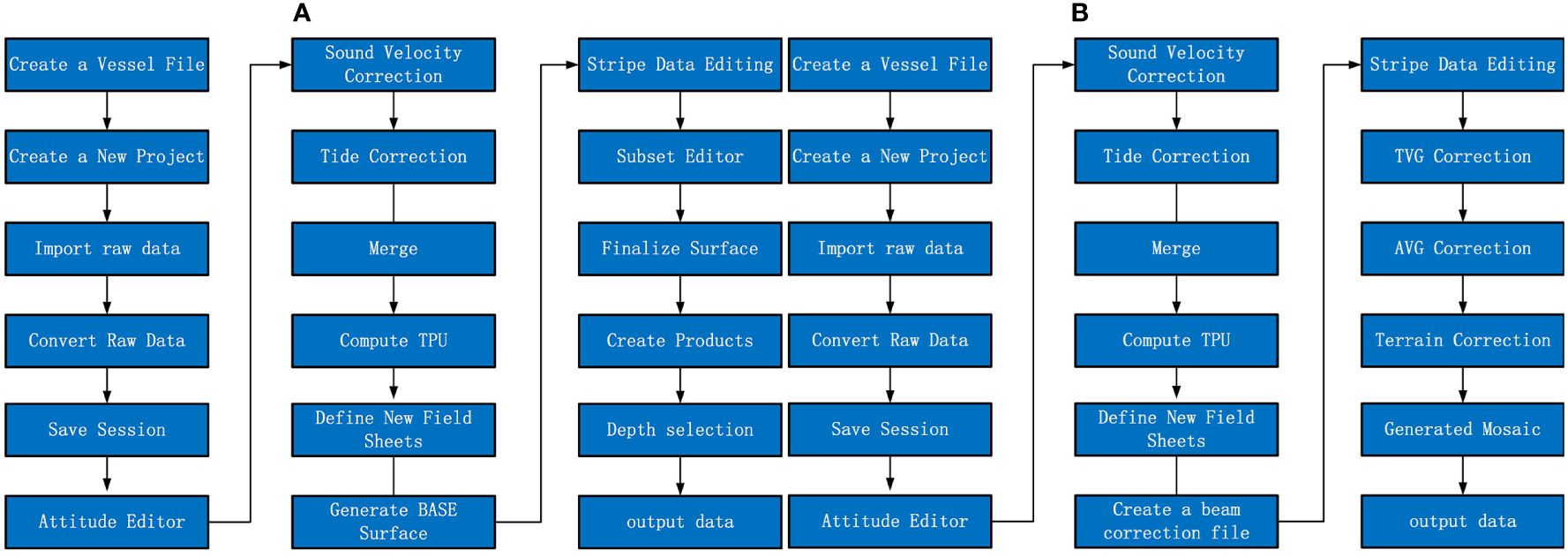
Figure 2 (A) Bathymetry data processing flow chart. (B) Backscatter data processing flow chart.

2.3 Typical machine learning algorithms

Machine learning commonly involves the tasks of classification and regression. The primary objective of the classification problem is to train a classification model using the attributes of the dataset including established categories, and thereafter identify the category rules in order to make predictions regarding the category to which the unknown data pertains. Some commonly used classification methods in machine learning include K-nearest neighbor (KNN), support vector machine, random forest, naive Bayes, and BP neural network, among others.

2.3.1 The K-nearest neighbor algorithm

The fundamental principle underlying the K-nearest neighbors (KNN) approach involves computing the distance between the item to be classified and every item inside the dataset using a distance metric. Subsequently, the K items with the closest distance are chosen. In the process of classification, the calculation involves determining the distance between each sample and the K items. The provided sample’s The classification of the sample will be chosen by the class that is closest to it.

2.3.2 Support vector machine

The Support Vector Machine (SVM) technique is a type of supervised learning used for both classification and regression tasks. The fundamental concept involves identifying a hyperplane within the training dataset. The hyperplane in question is sometimes referred to as a “interval zone” due to its ability to effectively segregate various data kinds.

2.3.3 BP neural network

A backpropagation neural network (BP neural network) is composed of an input layer, an output layer, and multiple hidden layers positioned between them. Upon forward propagation of the training data, the resulting structure will be communicated to the output layer subsequent to undergoing processing by the hidden layer. If there is a significant disparity between the outcomes and anticipated values, it is necessary to make reverse changes in order to establish the error weights for each unit.

2.3.4 Decision tree

The decision tree method is a fundamental mathematical technique used in machine learning. The process commences at the root node and progressively executes the most efficient partitioning of features until it reaches the leaf node in order to construct a tree structure. Every node corresponds to the evaluation of a characteristic. The fundamental objective of training is to construct a categorization. The classification of data sets is accomplished through the utilization of a tree structure.

2.3.5 Random forest

The random forest algorithm is a type of ensemble learning technique that is founded on the concept of bulk categorization. The fundamental premise of this approach involves the random selection of N samples from the training set, including replacement, in order to create a new training set. This new training set is then utilized to train multiple decision trees. A new classifier is created by combining many decision trees, and the final classification result is obtained by a voting process.

2.3.6 Extreme random tree

The algorithmic principles of the extreme random tree classification method and the random forest classification algorithm exhibit significant similarities, as both involve the utilization of multiple decision trees. The random forest algorithm employs a random sampling technique to select samples from the training set for each decision tree, whereas extreme random trees retain all samples in their training set. Due to the random nature of the split, the features are chosen in a random manner.

2.3.7 Gradient boosting tree

The gradient boosting tree is a machine learning approach that combines decision trees with other techniques. The approach employs a series of iterations to produce many weak classifiers. Each iteration aims to decrease the previous residual and in the process, it can create a new classifier. The novel weak classifier employs a continuous iterative process to mitigate bias, hence enhancing the overall accuracy of the final classifier.

2.3.8 XGBoost

XGBoost, short for Extreme Gradient Boosting, is a unified technique that builds upon the gradient boosting decision tree method. The fundamental concept of the method is Boosting, which combines numerous weak classifiers into a powerful learner in a certain manner. The XGBoost algorithm demonstrates superior performance and scalability compared to the gradient boosting tree. It achieves this by expanding the target Taylor to the second order, thereby capturing more information about the objective function. Additionally, the algorithm incorporates a regularization term in the objective function, which helps reduce model variance.

2.3.9 Adaptive enhanced classification

AdaBoost is a type of Boosting model that is used for adaptive boosting classification algorithms. This approach has the capability to construct several weak classifiers, in contrast to the Bagging model. The weak classifiers constructed in the subsequent round exhibit dissimilarities when compared to the weak classifiers constructed in the preceding round. The formation of a strong classifier is achieved through the continual construction of several weak classifiers, hence establishing dependencies.

2.3.10 Naive Bayes classification

The Naive Bayes classification method is a fundamental techniques for classification. The fundamental concept revolves around the computation of the probability associated with the respective category of sample attributes, with the highest probability being employed as the classification result. Given the assumption that the sample feature is a member of category y, the likelihood of the feature being associated with the category can be expressed as follows (Equation 1):

$\begin{array}{ll}\mathit{P}(\mathit{y}|{\mathit{x}}_{\mathbf{1}},{\mathit{x}}_{\mathbf{2}},{\mathit{x}}_{\mathit{n}})=\frac{\mathit{P}(\mathit{y})\mathit{P}({\mathit{x}}_{\mathbf{1}},{\mathit{x}}_{\mathbf{2}},\cdot \cdot \cdot {\mathit{x}}_{\mathit{n}}|\mathit{y})}{\mathit{P}({\mathit{x}}_{\mathbf{1}},{\mathit{x}}_{\mathbf{2}},{\mathit{x}}_{\mathit{n}})}& (1)\end{array}$

The above briefly introduces the basic definitions of common machine learning algorithms. These methods have their limitations and are suitable for different data sets. Therefore, this study uses the established western Pacific seamount dataset to compare and analyze the above-mentioned machine learning algorithms. It is very necessary to screen out the model algorithm that best suits this dataset. Please see below for details.

2.4 Feature extraction and screening

The mechanism of multi-beam sounding entails the initial stimulation of an acoustic pulse by the transmitting transducer, which then propagates towards the seafloor. When encountering an uneven seafloor interface, the acoustic impedance will increase due to the mutation of the propagation medium. Phenomena such as reflection and scattering give rise to the generation of echoes, which in turn yield three significant pieces of information: bathymetry data, backscatter data, and water column data. The bathymetry data is primarily utilized for the purpose of characterizing the topography and morphology of the seabed, as well as observing alterations in landforms. On the other hand, the backscatter data serves as a representation of the scattering and reflection signals emitted by the seabed medium, enabling the examination of the composition and spatial arrangement of the seabed substrate. For every beam, it is possible to record both a bathymetry value and a backscatter intensity value, which are directly related to the seafloor position coordinates.

The researchers are able to generate a high-precision digital elevation model (DEM) of the entire seamount by utilizing extensive multi-beam bathymetry data and employing a high-precision differential positioning technique. The Digital Elevation Model (DEM) utilizes a restricted amount of terrain elevation data to digitally replicate the terrain surface and accurately represent its form. The DEM is a digital representation that comprises extensive geomorphological data for the investigation of terrain features (Xiong et al., 2021). The DEM is a useful tool for visually representing the vertical distance between two sites and the average sea level. It has consistently been a significant tool in the analysis of geomorphological characteristics. Nevertheless, because of the intricate and dynamic nature of seabed terrain features, which exhibit varying sizes and shapes, even within the same landform category, the configurations of distinctive entities can vary significantly across different landform contexts (Anders et al., 2015). A Digital Elevation Model (DEM) is a digital representation of the topography of a terrain surface. DEM can be conceptualized as a three-dimensional vector, denoted by a set {X, Y, H}, where X represents the longitude and Y represents the latitude of a specific point within the DEM. The combined values of X and Y provide the location information of the DEM point, while H represents the elevation value of the point. Researchers typically extract latent characteristics that depict topographical attributes using DEM, and these latent characteristics are referred to as terrain factors. Terrain factors are specific physical parameters that represent the morphological properties of landforms. The correlation between seabed topography and the dispersion of seafloor substrates has been substantiated by numerous researchers. Hence, the acquisition of derived features that accurately depict topographic characteristics using DEM holds considerable importance in the field of substrate categorization (Lundblad et al., 2006; Holmes et al., 2008).

Currently, the technique for extracting terrain elements using Digital Elevation Models (DEM) is well-established. One of the more prevalent methods for obtaining terrain characteristics is through the utilization of ArcGIS. ArcGIS is a comprehensive software for processing geographic information, but it has limited efficiency in calculating terrain factors. To optimize the extraction of terrain factors in batches, this study utilizes the Arcpy library function in ArcGIS to analyze the processed DEM elevation model. Subsequently, the terrain factors that define the topography of the seabed are computed in batches. The Arcpy library encompasses a variety of geospatial processing modules, including but not limited to the raster analysis module and the map algebra operated module. The Arcpy library function allows for the calculation of terrain factors, like as slope and BPI (Lundblad et al., 2006), using various search radius values. The program thoroughly takes into account the topography of the deep sea. The integrity of landform units is ensured by the relative relationship between a single grid node and the surrounding grid nodes.

The association between the size of the backscatter and many physical parameters, including seabed roughness, sediment particle size, porosity, saturation, and incident angle, has been observed. The analysis of backscatter data not only provides insights into the reflection capacity of the deep seabed substrate type in response to incident sound energy, but also enables the extraction of diverse textural features that may be used to characterize the substrate type from various perspectives. The texture feature refers to the degree of roughness exhibited by the surface structure of the seabed. The brightness of the pixels in the backscatter mosaic image can be directly influenced by the textural characteristics of various seabed substrates. The backscatter mosaic refers to a grayscale image that is spatially referenced, whereas the texture features can be associated with the spatial statistical distribution of the grayscale image (Haralick et al., 1973). Currently, there exists a multitude of eigenvectors that characterize texture features, exhibiting distinct gray-level correspondences in their spatial distribution. The approach for estimating texture features based on the gray-level co-occurrence matrix of second-order statistics was proposed by R. Haralick in 1973 (Haralick et al., 1973). The gray co-occurrence matrix reveals the gray relationship between pixels through certain moving Windows and directions (0°, 45°, 90°, 135°). It is defined as the probability of the occurrence of gray value j is calculated from the pixel with gray value i in the given direction. The mathematical expression is as follows (Equation 2):

$\begin{array}{ll}\mathit{P}(\mathit{i},\mathit{j}|\mathit{d},\mathit{\theta })=\mathit{\#}\left\{(\mathit{x},\mathit{y})\right|\mathit{f}(\mathit{x},\mathit{y})=\mathit{i},\mathit{f}(\mathit{x}+\mathit{d}\mathit{x},\mathit{y}+\mathit{d}\mathit{y})=\mathit{j};\mathit{x},\mathit{y}=\mathbf{0},\mathbf{1},\mathbf{2}\cdot \cdot \cdot \mathit{L}-\mathbf{1}\}& (2)\end{array}$

The relative distance, denoted as d, is determined by the number of pixels. The calculating window movement direction, often represented by values of 0°, 45°, 90°, and 135°, is also included in the formula. The symbol “#” denotes a set. i,j = 0,1,2•••L-1;The pixel coordinates of the grayscale image are denoted as (x,y), while L represents the total number of grayscale levels present in the image.

The process of extracting backscatter grayscale images from the grayscale co-occurrence matrix is only a statistical outcome. To obtain more precise statistics, such as mean, variance, contrast, entropy, energy, correlation, homogeneity, etc., a sequence of weighted processes is necessary.

Various features are derived using the bathymetry data and backscatter data collected from the deep-water multi-beam bathymetry system. Each feature can depict the topography or underlying attributes from various perspectives. To minimize data redundancy, it is necessary to choose the least characteristic factors that may represent the largest amount of information for classification while minimizing the computational workload of the algorithm. Hence, it is imperative to evaluate the characteristics using quantitative analysis. Researchers frequently employ feature dimensionality reduction techniques such as factor analysis and maximum correlation-minimum redundancy (mRMR). It was the renowned psychologist Charles E. who initially introduced the factor analysis method. The method in question originated from the principal component analysis technique. The fundamental concept revolves around the examination and computation of the covariance relationship among different variables, the reduction of variable dimensionality, and the identification of a limited number of variables that effectively capture the majority of the original information contained within the variables (Spearman, 1961). The maximum correlation-minimum redundancy method guarantees the highest possible correlation between features and categories while also ensuring the lowest possible redundancy among the selected characteristics. It takes into account not just the correlation between features and categories, but also the correlation between features themselves (Peng et al., 2005). In order to select a feature screening method suitable for this data set, the above two feature screening methods are compared and analyzed below.

3 Experiments and results

3.1 Construction of the data set

This article classifies the seabed bottom in the research region into six distinct types, namely: (1) Bedrock, (2) Crust, (3) Nodules, (4) Gravel, (5) Calcareous substrates, and (6) Gravel substrates, based on on-site reports, sampling data, and video visual displays. Photographs depicting the comparable patterns of the six deep-sea seamount substrates are presented in Figure 3. Based on the drilling findings pertaining to the Caiwei Seamount, the predominant geological composition within the seamount region comprises basalt, breccia, volcaniclastic rock, and limestone. Pillow basalt and huge basalt are mostly generated through the process of lava eruption from the seafloor followed by subsequent cooling. The hue often ranges from black to dark gray. Breccia exhibits a gray-black hue and typically consists of volcanic debris or encrusted fragments, typically measuring between 2 and 4 cm in particle size. The predominant composition of volcaniclastic rocks consists of basalt fragments, characterized by their irregular rhombus and spherical shapes. Crusts predominantly exhibit a black or gray-black coloration, and can be categorized into plate-shaped crusts, granular crusts, and cobalt nodules based on their respective morphologies. The majority of nodules have a black or brown-black coloration, with a predominant round or oval shape. Based on their diameter, nodules can be categorized into three groups: tiny nodules (with a diameter of less than 3cm), medium nodules (with a diameter of 3-6cm), and giant nodules (with a diameter exceeding 6cm). According to the particle size classification table of the isometric system (φ value standard), the particle diameter of gravel is less than 256 mm. Gravel can be divided into coarse gravel (64-256 mm), medium gravel (8-64 mm), and fine gravel (2-8 mm) according to the particle diameter (Folk et al., 1970). Due to the limited resolution of optical video, foraminifera sand, calcareous mud and calcareous sand are classified as calcareous substrates in this paper; coarse gravel, medium gravel and fine gravel are classified as gravel; referring to the FOLK classification standard, some substrates containing gravel are defined as gravelly substrates; some clay is located under the surface of nodules, and clay and nodules are defined as nodule areas in this paper; different forms of crusts are defined as crust areas.

Figure 3

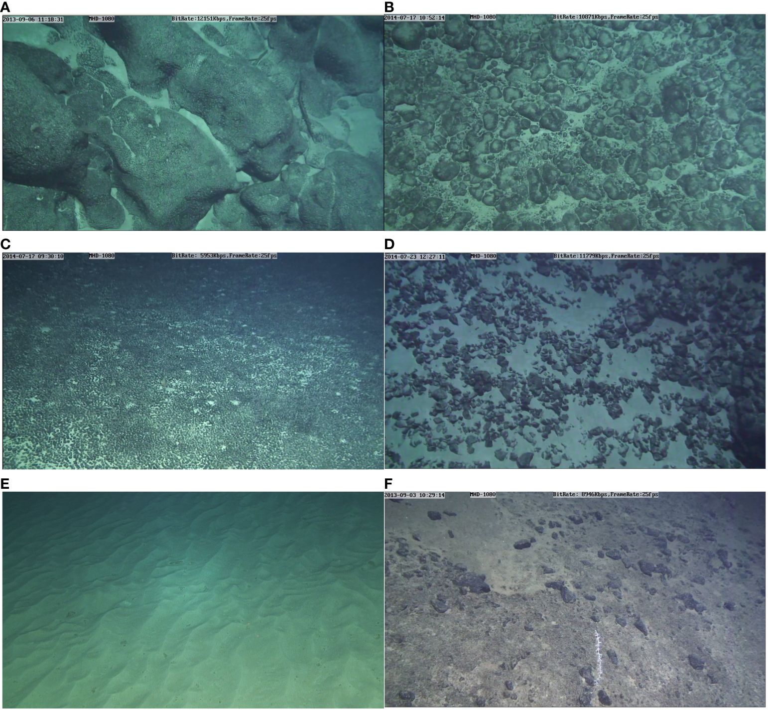
Figure 3 Substrate type pattern diagram in seamount area. (A) bedrock; (B) Crust; (C) Nodules; (D) Gravel; (E) Calcium sediments; (F) Gravel sediments.

In order to simplify the process of manually interpreting the different bottom kinds in the video, this paper provides categorization labels for the six bottom types found in the research region. Only the initial time point, final time point, and classification label of each bottom type need to be recorded during the recording procedure. The Jiaolong manned submersible has a consistent underwater cruising speed of 1 knot, allowing it to cover an average distance of around 30.8 m/min. This research posits that the duration between the initiation and conclusion of the bottom type is shorter than 5 minutes, similar to the preceding bottom type. An algorithm is employed to automatically populate all label values within a time span of 100 seconds after manually analyzing the footage obtained from all dives. The algorithm is utilized to align the processed ultra-short baseline positioning data based on the time value associated with each label value, resulting in the classification point set for the bottom type of the seamount area. The classification point set consists of multiple points (X, Y, T), where (X, Y) represents the geographic coordinates of each classification label point. X denotes the longitude of each classification label point, Y denotes the latitude of each classification label point, and T represents the classification label of each point. A preliminary set of 8,179 data points, divided into 6 categories, was generated by manually analyzing the video footage from all dives. The continuous seafloor information was transformed from a point-based representation to a line-based representation. By utilizing the bathymetry and backscatter data obtained from the deep-water MBES system, it is possible to depict the “surface” characteristics of the study area. This data enables the prediction and classification of the bottom conditions across the entire seamount area, facilitating a comprehensive analysis that progresses from “points” to “lines” and ultimately to “surfaces”.

3.2 Extraction of features

The multi-beam sounding system in deepwater has the capability to acquire both high-resolution bathymetry data and high-resolution backscatter data, with each data point being associated with a specific location. This article employs ArcGIS to achieve data size consistency during feature matching by initially cropping the bathymetry data and backscatter data to same dimensions. Subsequently, the cropped backscatter data is exported as a grayscale image. This work use the gray level co-occurrence matrix approach to extract statistics in four directions (0°, 45°, 90°, 135°) using a 5*5 sliding window with a moving step of 4. The algorithm is then utilized to merge the four directions. The average statistics are calculated by averaging the statistics in several directions, resulting in the final characterization of texture features. The technique utilizes the backscatter grayscale image to extract a total of 8 features, including mean, variance, homogeneity, dissimilarity, entropy, energy, correlation, and auto-correlation (Haralick et al., 1973). The part of Caiwei Seamount textural features is depicted in Figure 4. The analysis of Figure 4 reveals that each feature quantity effectively represents the structure, distribution information, and gray-scale relationship among pixels in Caiwei Seamount grayscale picture points captured from various angles. However, not all feature quantities are used for bottom classification research. In order to avoid data redundancy, further feature screening is required later. For details, see Section 3.4 model evaluation in this article.

Figure 4

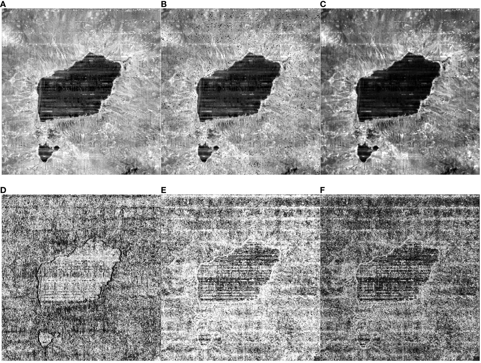
Figure 4 Caiwei seamount texture feature quantity. (A) Grayscale image; (B) Mean; (C) Variance; (D) Homogeneity; (E) Entropy; (F) Auto_correlation.

According to the user’s scale factor, the bathymetric position index (BPI) can be categorized into two types: Broad-scale BPI (Broad Bathymetric Position Index, B-BPI) and fine-scale BPI (Fine Bathymetric Position Index, F-BPI). The deep position index quantifies the relative variations in elevation among landform units at both macroscopic and microscopic levels. The scale factor of the bathymetry position index (BPI) is determined by multiplying the resolution of the bathymetry data by the outer radius of the BPI. The trial and error method is presently the prevailing approach for identifying the suitable scale factor. However, it is important to note that this method does compromise categorization efficiency to some degree. DILLON believes that the size of the scale factor should be roughly the same as the identified landform feature. Therefore, the width of the landform unit can be roughly measured to roughly obtain the trial and error range and improve the efficiency of trial and error (Dillon, 2016). For example, if the ridge width is 500m and the bathymetric resolution is 2m, the outer radius is defined as 250, thus obtaining a scale factor of 500, and the inner radius is usually defined as one tenth of the outer radius (Dillon, 2016). The outer radius has a value of 250. This study employed the BPI definition to initially assess the dimensions of the geomorphological units of interest within the western Pacific seamount region. Additionally, it aimed to ascertain the trial and error range of the terrain scale factor. After conducting numerous experiments, this study determined that an outer radius of 325 and an inner radius of 33 are suitable for calculating the broad-scale bathymetric position index (B-BPI) of the Caiwei Seamount. Similarly, for the fine-scale bathymetric position index (F-BPI) of the Caiwei Seamount, an outer radius of 6 and an inner radius of 3 were selected. The Arcpy library function automatically generates many terrain factors that describe terrain characteristics, including Broad-scale BPI, slope, VRM (Horn, 1981), and more. Figure 5 displays several terrain characteristics.

Figure 5

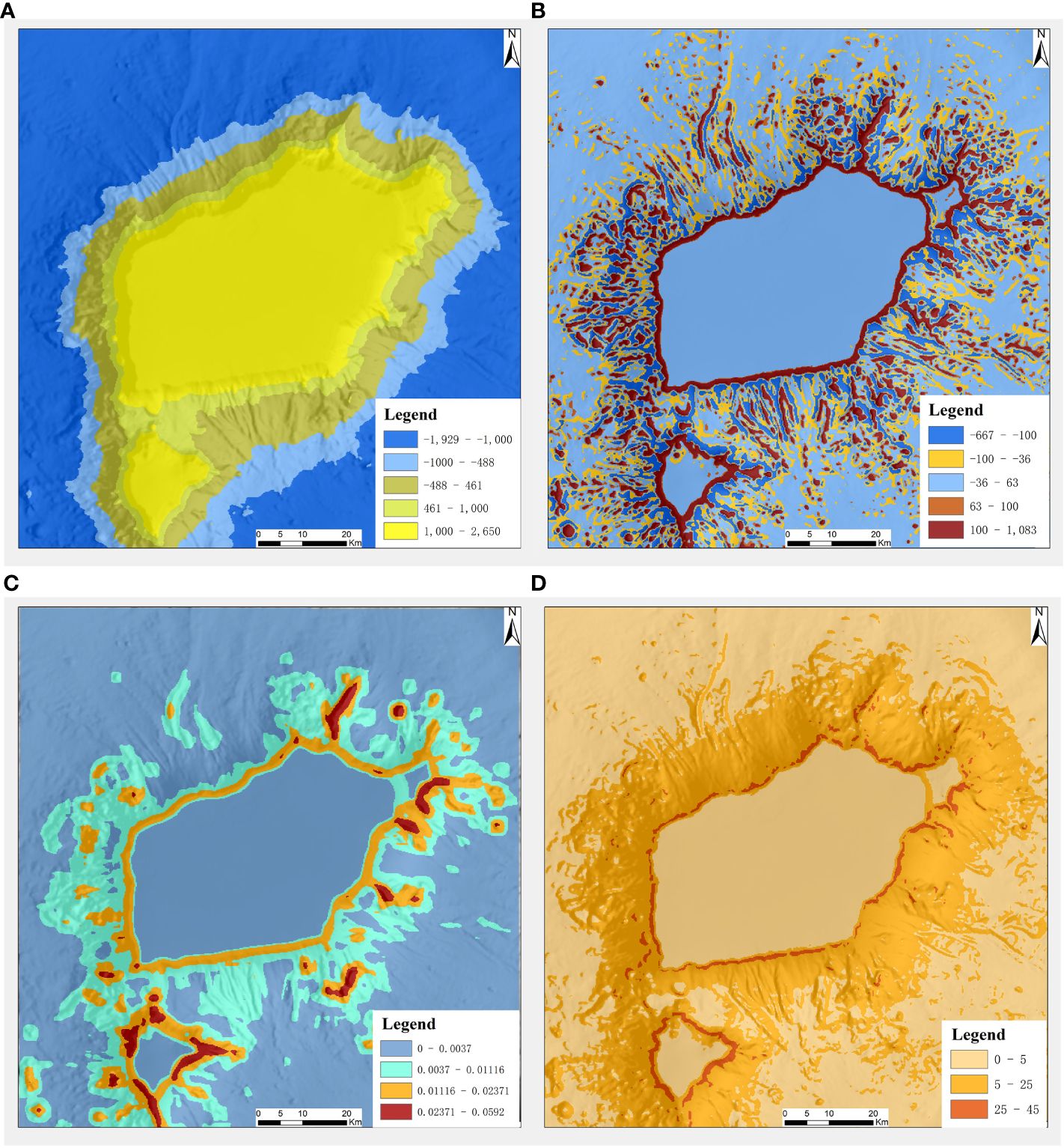
Figure 5 Terrain factor. (A) B-BPI; (B) F-BPI; (C) VRM; (D) Slope.

3.3 Matching of features

The deep-sea bottom substrate types are characterized by extracting various distinctive variables using bathymetry data and backscatter data taken by MBES technology. The key to achieving automatic classification of seamount substrates lies in establishing the relationship between each substrate type and its characteristic factors. This paper uses video data collected by the “Jiaolong” manned submersible. The visual range of the video data is less than 30m and the data resolution acquired by deep-water multi-beam is low. To determine the substrate type, this paper assumes that the time interval between the start and end of the substrate type is less than 5 minutes. The algorithm records a classification point set every 100 seconds. The established classification point set, as mentioned earlier, consists of (X, Y, T) where (X, Y) represents the geographic coordinates of each classification label point. X denotes the longitude and Y denotes the latitude of each classification label point. T represents the classification label assigned to each point. Not all photo classification points (X, Y) in the classification point set can precisely correlate to the grid point of each feature. This paper employs the bilinear interpolation method to establish the correspondence between eigenvalues and each photo classification point (X, Y, T). The eigenvalues corresponding to each photo classification point (X, Y) are determined by considering the four grid points in the terrain factors. Figure 6 illustrates the fundamental premise. Given the photo classification point set Z (x, y), we have the coordinates of points Q₁₁, Q₁₂, Q₂₁, and Q₂₂ of the terrain factor. To begin, do interpolation in the X direction to calculate Z₁ and Z₂. Then, proceed to interpolate in the Y direction to get the eigenvalues that correspond to the classification point set Z (x, y). The calculating formula is as follows (Equations 3–5):

Figure 6

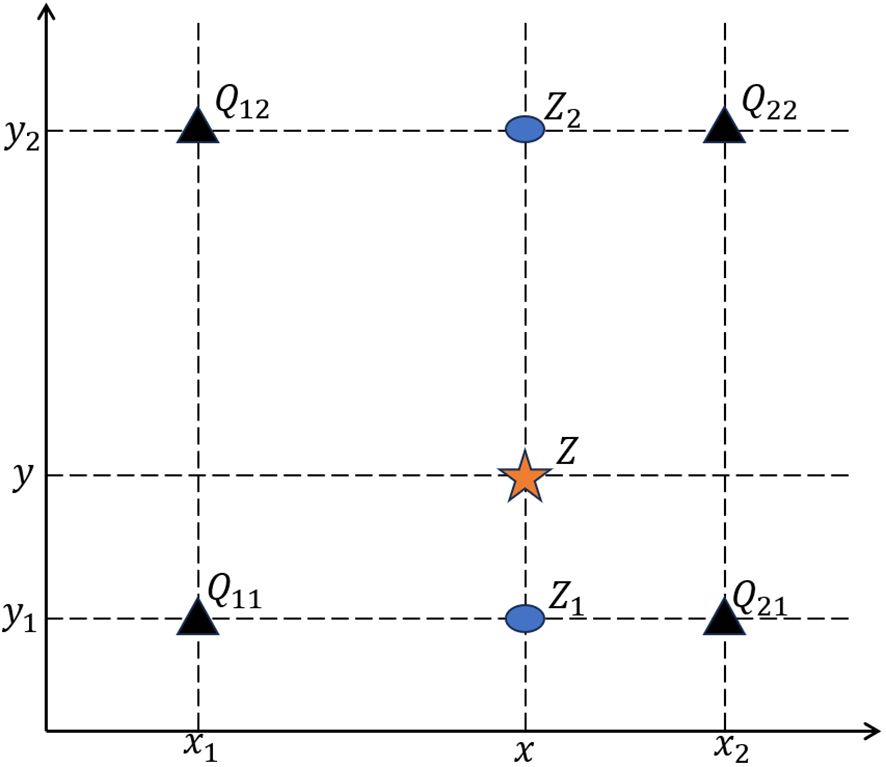
Figure 6 Schematic diagram of bilinear interpolation calculation.

$\begin{array}{ll}\mathit{f}({\mathit{Z}}_{\mathbf{1}})\approx \frac{{\mathit{x}}_{\mathbf{2}}-\mathit{x}}{{\mathit{x}}_{\mathbf{2}}-{\mathit{x}}_{\mathbf{1}}}\mathit{f}({\mathit{Q}}_{\mathbf{11}})+\frac{\mathit{x}-{\mathit{x}}_{\mathbf{1}}}{{\mathit{x}}_{\mathbf{2}}-{\mathit{x}}_{\mathbf{1}}}\mathit{f}({\mathit{Q}}_{\mathbf{21}})& (3)\end{array}$

$\begin{array}{ll}\mathit{f}({\mathit{Z}}_{\mathbf{2}})\approx \frac{{\mathit{x}}_{\mathbf{2}}-\mathit{x}}{{\mathit{x}}_{\mathbf{2}}-{\mathit{x}}_{\mathbf{1}}}\mathit{f}({\mathit{Q}}_{\mathbf{12}})+\frac{\mathit{x}-{\mathit{x}}_{\mathbf{1}}}{{\mathit{x}}_{\mathbf{2}}-{\mathit{x}}_{\mathbf{1}}}\mathit{f}({\mathit{Q}}_{\mathbf{22}})& (4)\end{array}$

After getting Z₁ and Z₂, get Z

$\begin{array}{ll} \mathit{f}(\mathit{Z})\approx \frac{{\mathit{y}}_{\mathbf{2}}-\mathit{y}}{{\mathit{y}}_{\mathbf{2}}-{\mathit{y}}_{\mathbf{1}}}\mathit{f}({\mathit{R}}_{\mathbf{1}})+\frac{\mathit{y}-{\mathit{y}}_{\mathbf{1}}}{{\mathit{y}}_{\mathbf{2}}-{\mathit{y}}_{\mathbf{1}}}\mathit{f}({\mathit{R}}_{\mathbf{2}})& (5)\end{array}$

Interpolation can be used to acquire the feature values, while the algorithm extracts the terrain factor values for the classification point sets in batches. The program then establishes the association between each classification point set and the feature factors.

This study used the feature matching technique to establish correspondences between a comprehensive set of 17 distinct characteristic parameters, encompassing terrain factors, backscatter, and texture feature quantities. The dataset consists of 8179 sediment categorization point sets. Of all the components, bedrock and crust make up a significant part, and the data is somewhat imbalanced. It can lead to suboptimal performance in machine learning categorization. In order to address this issue, the RandomOverSampler technique is employed in this article to resample the classification point set and attain data equilibrium. Following the process of resampling, the dataset comprises a total of 18,534 substrate categorization point sets, encompassing a comprehensive set of 17 features.

3.4 Model evaluation

It is evident from the aforementioned information that numerous machine learning algorithm models exist for the purpose of addressing classification problems. However, it is important to note that certain classification algorithm models are well-suited for specific types of data sets. In situations involving classification problems, it is customary to perform comparison analysis and screening of multiple classification models. Identify an appropriate categorization model for the given dataset. Hence, to evaluate algorithm models appropriate for this dataset, this part examines and contrasts the 10 prevalent classification approaches mentioned earlier.

In this section, the classification model is constructed using the training set, with a data set partition ratio of 4:1 between the training set and the test set. Cross-validation was employed to train all models, and the model hyperparameters were set to their default settings. Accuracy and recall are the evaluation indicators employed in this part, as they are often utilized in categorization assignments. The methods they use for calculating are as follows (Equations 6, 7):

Accuracy pertains to the ratio of accurately categorized sample points by the classification algorithm in relation to the total number of sample points.

$\begin{array}{ll} \mathit{\text{Accuracy}}=\frac{\mathit{T}\mathit{P}+\mathit{T}\mathit{N}}{\mathit{T}\mathit{P}+\mathit{T}\mathit{N}+\mathit{F}\mathit{P}+\mathit{F}\mathit{N}}=\frac{\mathit{\text{Number of correctly classified samples}}}{\mathit{\text{All sample numbers}}} & (6)\end{array}$

The concept of recall pertains to the ratio of accurately identified samples to the total number of positive samples.

$\begin{array}{ll}\mathit{\text{Recall}}= \frac{\mathit{T}\mathit{P}}{\mathit{T}\mathit{P}+\mathit{F}\mathit{N}}= \frac{\mathit{\text{Number of correctly classified positive samples}}}{\mathit{\text{Number of true positive samples}}}& (7)\end{array}$

The variable TP represents the count of positive samples that were accurately identified by the classification algorithm. The variable TN represents the count of negative samples that were accurately categorized by the classification algorithm. The variable FP represents the count of negative samples that were erroneously categorized as positive samples by the classification algorithm. FN is the number of positive samples that are mistakenly classified as negative samples by the classification algorithm.

This section aims to objectively assess 10 commonly employed classification algorithms using accuracy and recall rates. The objective is to identify classifiers that exhibit exceptional classification performance in classifying deep-sea seamount deposits. To ensure a precise evaluation of the algorithm’s adaptive capability, the training set employed in this experiment did not employ the feature screening technique for data filtering. Instead, a total of 17 feature factors were utilized as input. Table 2 displays the categorization outcomes of the ten classification algorithms.

Table 2

Table 2 Classification effects of 10 common classification algorithms.

The table clearly demonstrates that the decision tree, extreme random tree, and XGBoost classification algorithms achieve an accuracy above 0.88 for deep-sea seamount bottom classification. Additionally, the recall rate exceeds 0.87. Hence, this part opts for decision tree, extreme random tree, and XGBoost to carry out the subsequent experiment.

The initial step in selecting an improved feature screening approach involves employing factor analysis to compute the Pearson correlation coefficient between each pair of the 17 features. In cases when features are highly associated, certain features can be eliminated in order to minimize the need for additional feature screening. Superfluous data, as illustrated in Table 3. According to this article, it is posited that characteristics exhibit a high level of connection when the Pearson correlation coefficient exceeds 0.6. Ultimately, the eight features presented in Table 3 exhibit a low level of correlation. This part employs mRMR to eliminate 8 feature factors from a total of 17 features. These factors are ordered in order of relevance as follows: bathymetry, backscatter, slope, ruggedness, mean, variance, broad-scale BPI, and fine-scale BPI. The purpose is to ensure consistency in the amount of features throughout following tests. This part employs cross-validation of two feature screening approaches with three classifiers to ascertain an improved classification model. Table 4 displays the results. The mRMR-XGBoost model has the highest classification accuracy and recall rate under the same feature data set, and the model classification accuracy is 92.5%, an increase of 2 percentage points. Therefore, the mRMR feature screening method is more suitable for this data set, with obvious advantages. The mRMR-XGBoost classification model can better realize the automatic classification of deep-sea seamounts.

Table 3

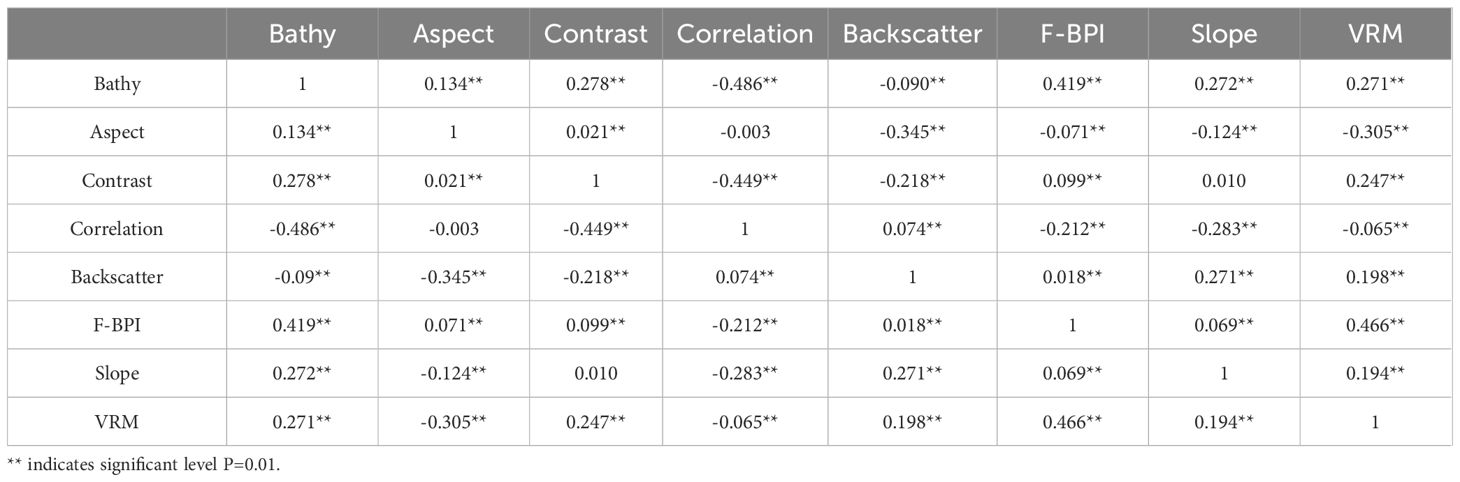
Table 3 Pearson correlation coefficient between different features.

Table 4

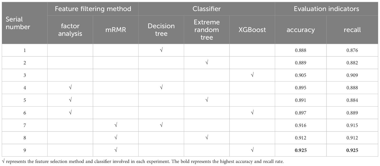
Table 4 Feature screening method and classifier cross-validation results.

3.5 Model application and post-processing

To assess the classification performance of the mRMR-XGBoost model, this section applies the model to the deep sea Caiwei Seamount and generates a confusion matrix of the prediction results on the validation set (Krstinić et al., 2020). The confusion matrix is presented in Figure 6. The model accurately classifies the substrate type, and the associated dark color blocks are evenly dispersed along the diagonal. Figure 7 clearly demonstrates that the categorization accuracy for each category is notably high, particularly for nodules and gravel deposits. The overall classification impact is enhanced and can more accurately differentiate the substrate type of deep-sea seamounts. Using Caiwei Seamount as an illustration, Figure 8A displays the initial classification outcome of the model for Caiwei Seamount. The figure clearly demonstrates the mRMR-XGBoost model’s ability to accurately distinguish substrate types, however there are some instances of noise present in the image. To ensure the preservation of substrate continuity. The present section employs the ArcGIS geoprocessing platform for the purpose of reclassifying the data obtained from sediment classification. The substrate distribution of Caiwei Seamount after reclassification is depicted in Figure 8B. The Ocean 80 expedition collected data on the Caiwei Seamount using two box sampling sites, BC08 and BC09. Figure 8B displays the positions of the two stations. The image illustrates that the two stations are situated directly on the seafloor, specifically in the western region of the Caiwei Seamount. The sampling findings in the plain area are depicted in Figures 9A, B. The two observed outcomes in the sampling are nodules and clay. The two stations are situated inside the nodular area depicted in Figure 9B. The mRMR-XGBoost model has a high level of accuracy and achieves favorable classification outcomes.

Figure 7

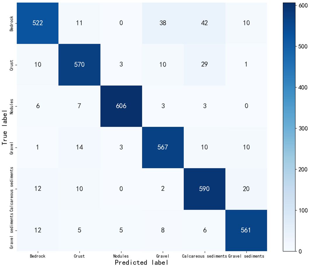
Figure 7 Confusion matrix between mRMR-XGBoost model predicted labels and true labels.

Figure 8

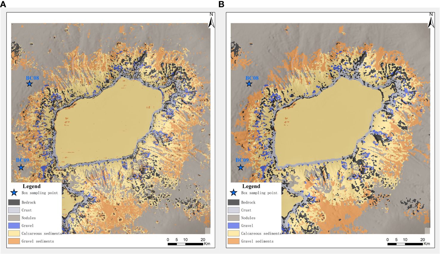
Figure 8 Caiwei seamount substrate classification thematic map. (A) Not reclassified; (B) Reclassified.

Figure 9

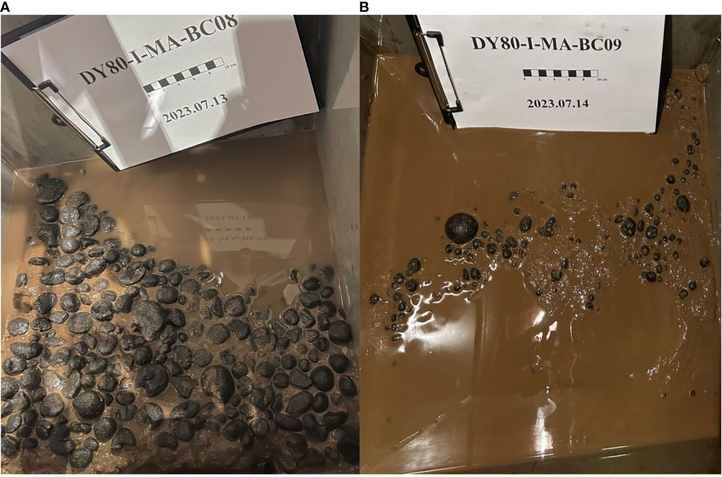
Figure 9 Caiwei seamount box sampling map. (A) Station BC08; (B) Station BC09.

4 Discussions

With the continuous increase in the amount of acoustic and optical data, the application of machine learning in substrate classification has gradually increased. However, since a large number of real labels are required when building machine learning models, the deep-sea environment is relatively complex. Compared with shallow water multi-beam data, deep-sea multi-beam data is not easy to obtain, and deep-sea substrate classification labels are insufficient. Therefore, most substrate classification models are applied to offshore, and are less used in deep sea. In view of the problem of insufficient deep-sea substrate classification labels and low accuracy, this paper defines 6 types of sediments, such as bedrock and crust, based on ocean voyage reports and sampling results. In-situ videos collected by the Jiaolong manned submersible were deeply mined, 25 submersible survey lines were manually interpreted, and a classification point set of the western Pacific seamount area was established through the start and end time points of each sediment type for training substrate classification models. Subsequent work can establish a rich image data set, use artificial intelligence technologies such as image recognition instead of manual interpretation to reduce human subjectivity, and further optimize the classification data set. Based on the acoustic data mining hidden features obtained from deep-water multi-beam data, a total of 17 characteristic factors were extracted using the algorithm, including topographic factors, texture features, etc., as shown in Figures 4, 5. Subsequent work can mine deeper characteristic factors for more detailed characterization of the bottom characteristics of deep-sea seamount areas.

At present, there are many commonly used machine learning models, but different models are suitable for different data sets. In order to screen out the model suitable for this data set, this paper uses 17 feature factors to test the applicability of each machine learning classification model, and uses recall and accuracy to evaluate the model performance, as shown in Table 2. This paper screens out 3 classifiers with an accuracy of more than 88%. In order to further improve the model performance and avoid data redundancy, this paper uses factor analysis and maximum relevance-minimum redundancy (mRMR) to screen the most representative feature factors from the 17 feature factors, as shown in Table 3. The feature screening method is combined with the three classifiers with better performance determined in the previous article and a cross-validation experiment is completed, as shown in Table 4. From the previous experiments, we can see that the mRMR-XGBoost classification model is more suitable for this data set. As shown in Table 4 the model improves the accuracy of bottom classification from 90.05% to 92.5%, and the classification efficiency is further improved. From the actual box sampling results, we can see that the classification effect of the mRMR-XGBoost model is relatively accurate, but the model still has room for improvement. The mRMR model only outputs the order of importance of the feature factors, but the XGBoost model trains the model according to the same degree of importance, and does not give the feature factors a certain training weight. Subsequent research work can give training weights to different feature factors to further optimize the classification model, and the classification accuracy still has room for improvement. In terms of classification model verification, due to the high cost of obtaining seabed bottom samples in deep-sea environments and the small number of model verification samples, the relevant bottom classification areas can be sampled and verified in the subsequent voyage design to further verify the effectiveness of the model classification. When constructing the classification data set, this paper only considered the relationship between the bottom type and the backscatter intensity, topography, and texture features, and does not consider the relationship between the bottom type and the backscatter response curve (AR). In the following work, the relationship between the deep-sea seamount bottom type and the backscatter intensity, topography and backscatter response curve (AR) can be fully considered.

5 Conclusion

The seafloor, serving as a significant geological interface between the hydrosphere, biosphere, and lithosphere, harbors abundant mineral and biological resources. Hence, it is imperative to comprehend the spatial arrangement of seabed substrate types in order to effectively harness seabed resources [35]. This paper conducted research on the substrate classification method of deep-sea seamounts using deep-water multi-beam data and video data collected by the “Jiaolong” manned deep submersible. Through manual interpretation, a set of substrate classification points in the seamounts was established. The issue of inadequate classification labels is addressed by proposing the mRMR-XGBoost substrate classification model. The model achieves a substrate classification accuracy of 92.5%, indicating its strong suitability for this particular data set. The mRMR-XGBoost substrate classification model demonstrates a sediment classification accuracy of 92.5% when combined with the ocean box sample findings. The utilization of a quality classification model has proven to be a successful approach in facilitating sediment classification tasks, particularly in the context of coastal and mountainous regions. The present study utilizes acoustic data and in-situ video data to accomplish the automated classification of sediments found in deep-sea seamounts. This research offers fundamental assistance in investigating the distribution patterns of deep-sea seamount sediments.

Data availability statement

The original contributions presented in the study are included in the article/supplementary material. Further inquiries can be directed to the corresponding author.

Author contributions

DH: Writing – original draft, Data curation, Methodology, Software. YS: Conceptualization, Formal analysis, Resources, Supervision, Writing – review & editing. WG: Formal analysis, Project administration, Resources, Writing – review & editing. WX: Funding acquisition, Supervision, Validation, Writing – review & editing. WW: Validation, Visualization, Writing – review & editing. YZ: Investigation, Validation, Writing – review & editing. LW: Formal analysis, Validation, Visualization, Writing – review & editing.

Funding

The author(s) declare financial support was received for the research, authorship, and/or publication of this article. This research was supported by the National Key Research and Development Program of China (No.2023YFC2812903). This research was supported by the National Key Research and Development Program of China (No.2022YFC2808305).

Conflict of interest

The authors declare that the research was conducted in the absence of any commercial or financial relationships that could be construed as a potential conflict of interest.

Publisher’s note

All claims expressed in this article are solely those of the authors and do not necessarily represent those of their affiliated organizations, or those of the publisher, the editors and the reviewers. Any product that may be evaluated in this article, or claim that may be made by its manufacturer, is not guaranteed or endorsed by the publisher.

References

Alevizos E., Snellen M., Simons D. G., Siemes K., Greinert J. (2015). Acoustic discrimination of relatively homogeneous fine sediments using bayesian classification on mbes data. Mar. Geol 370, 31–42. doi: 10.1016/j.margeo.2015.10.007

CrossRef Full Text | Google Scholar

Anders N. S., Seijmonsbergen A. C., Bouten W. (2015). Rule set transferability for object-based feature extraction: an example for cirque mapping. Photogrammetric Eng. Remote Sens. 81, 507–514. doi: 10.14358/PERS.81.6.507

CrossRef Full Text | Google Scholar

Biot M. A. (2005). Theory of propagation of elastic waves in a fluid-saturated porous solid. Ii. Higher frequency range. J. Acoustical Soc. America 28, 179–191. doi: 10.1121/1.1908241

CrossRef Full Text | Google Scholar

CARIS (2016). CARIS HIPS & SIPS 9.1 User Guide.

Google Scholar

Chunhui T., Xiaobing J., Aifei B., Hongxing L., Xianming D., Jianping Z., et al. (2015). Estimation of manganese nodule coverage using multi-beam amplitude data. Mar. Geores Geotechnol 33, 283–288. doi: 10.1080/1064119X.2013.806973

CrossRef Full Text | Google Scholar

Dillon C. (2016). Modelling submerged coastal environments: remote sensing technologies, techniques, and comparative analysis is a book and lacks information such as the name of the corresponding school.

Google Scholar

Du D., Ren X., Yan S., Shi X., Liu Y., He G. (2017). An integrated method for the quantitative evaluation of mineral resources of cobalt-rich crusts on seamounts. Ore Geol Rev. 84, 174–184. doi: 10.1016/j.oregeorev.2017.01.011

CrossRef Full Text | Google Scholar

Fakiris E., Rzhanov Y., Zoura D. (2012). On importance of acoustic backscatter corrections for texture-based seafloor characterization.

Google Scholar

Folk R. L., Andrews P. B., Lewis D. W. (1970). Detrital sedimentary rock classification and nomenclature for use in New Zealand. New Z. J. geology geophysics 13, 937–968. doi: 10.1080/00288306.1970.10418211

CrossRef Full Text | Google Scholar

Gaida T. C., Mohammadloo T. H., Snellen M., Simons D. G. (2020). Mapping the seabed and shallow subsurface with multi-frequency multibeam echosounders. Remote Sens. (Basel Switzerland) 12, 52. doi: 10.3390/rs12010052

CrossRef Full Text | Google Scholar

Gan Y., Ma X., Luan Z., Yan J. (2021). Morphology and multifractal features of a guyot in specific topographic vicinity in the caroline ridge, west pacific. J. Oceanol Limnol 39, 1591–1604. doi: 10.1007/s00343-021-0383-8

CrossRef Full Text | Google Scholar

Haralick R. M., Shanmugam K., Dinstein I. H. (1973). Textural features for image classification. IEEE Trans. Syst. Man Cybernet. smc-3 (6), 610–621. doi: 10.1109/TSMC.1973.4309314

CrossRef Full Text | Google Scholar

Herzfeld U. C., Higginson C. A. (1996). Automated geostatistical seafloor classification—principles, parameters, feature vectors, and discrimination criteria. Comput. Geosci 22, 35–52. doi: 10.1016/0098-3004(96)89522-7

CrossRef Full Text | Google Scholar

Holmes K. W., Van Niel K. P., Radford B., Kendrick G. A., Grove S. L. (2008). Modelling distribution of marine benthos from hydroacoustics and underwater video. Cont Shelf Res. 28, 1800–1810. doi: 10.1016/j.csr.2008.04.016

CrossRef Full Text | Google Scholar

Horn B. K. P. (1981). Hill shading and the reflectance map. Proc. IEEE Inst Electr Electron Eng. 69, 14–47. doi: 10.1109/PROC.1981.11918

CrossRef Full Text | Google Scholar

Jackett C., Althaus F., Maguire K., Farazi M., Scoulding B., Untiedt C., et al. (2023). A benthic substrate classification method for seabed images using deep learning: application to management of deep-sea coral reefs. J. Appl. Ecol. 60, 1254–1273. doi: 10.1111/1365-2664.14408

CrossRef Full Text | Google Scholar

Ji X., Yang B., Tang Q. (2020). Seabed sediment classification using multibeam backscatter data based on the selecting optimal random forest model. Appl. Acoust 167, 107387. doi: 10.1016/j.apacoust.2020.107387

CrossRef Full Text | Google Scholar

Krstinić D., Braović M., Šerić L., Božić-Štulić D. (2020). Multi-label classifier performance evaluation with confusion matrix. Comput. Sci. Inf. Technol. 1, 1–14. doi: 10.5121/csit.2020.1008

CrossRef Full Text | Google Scholar

Lundblad E. R., Wright D. J., Miller J., Larkin E. M., Rinehart R., Naar D. F., et al. (2006). A benthic terrain classification scheme for american Samoa. Mar. Geod 29, 89–111. doi: 10.1080/01490410600738021

CrossRef Full Text | Google Scholar

Mancini D., Girardclos S., Lane S. N. (2020). Echoboat and hypack: user guide, Vol. 1.0.

Google Scholar

Mayer L., Jakobsson M., Allen G., Dorschel B., Falconer R., Ferrini V., et al. (2018). The nippon foundation—gebco seabed 2030 project: the quest to see the world’s oceans completely mapped by 2030. Geosciences (Basel) 8, 63. doi: 10.3390/geosciences8020063

CrossRef Full Text | Google Scholar

Mbani B., Schoening T., Gazis I., Koch R., Greinert J. (2022). Implementation of an automated workflow for image-based seafloor classification with examples from manganese-nodule covered seabed areas in the central pacific ocean. Sci. Rep. 12, 15338. doi: 10.1038/s41598-022-19070-2

PubMed Abstract | CrossRef Full Text | Google Scholar

Mbani B., Schoening T., Greinert J. (2023). Automated and integrated seafloor classification workflow (ai-scw). doi: 10.3289/SW_2_2023

CrossRef Full Text | Google Scholar

Michalopoulou Z., Alexandrou D., de Moustier C. (1995). Application of neural and statistical classifiers to the problem of seafloor characterization. IEEE J. Ocean Eng. 20, 190–197. doi: 10.1109/48.393074

CrossRef Full Text | Google Scholar

Müller R. D., Overkov N. C., Royer J. Y., Dutkiewicz A., Keene J. B. (1997). Seabed classification of the south tasman rise from simrad em12 backscatter data using artificial neural networks. Aust. J. Earth Sci. 44, 689–700. doi: 10.1080/08120099708728346

CrossRef Full Text | Google Scholar

Peng H., Long F., Ding C. (2005). Feature selection based on mutual information: criteria of max-dependency, max-relevance, and min-redundancy. IEEE Trans. Pattern Anal. Mach. Intell. 27, 1226–1238. doi: 10.1109/TPAMI.2005.159

PubMed Abstract | CrossRef Full Text | Google Scholar

Pillay T., Cawthra H. C., Lombard A. T. (2020). Characterisation of seafloor substrate using advanced processing of multibeam bathymetry, backscatter, and sidescan sonar in table bay, South Africa. Mar. Geol 429, 106332. doi: 10.1016/j.margeo.2020.106332

CrossRef Full Text | Google Scholar

Porskamp P., Rattray A., Young M., Ierodiaconou D. (2018). Multiscale and hierarchical classification for benthic habitat mapping. Geosciences (Basel) 8, 119. doi: 10.3390/geosciences8040119

CrossRef Full Text | Google Scholar

Rende S. F., Bosman A., Di Mento R., Bruno F., Lagudi A., Irving A. D., et al. (2020). Ultra-high-resolution mapping of posidonia oceanica (l.) Delile meadows through acoustic, optical data and object-based image classification. J. Mar. Sci. Eng. 8, 647. doi: 10.3390/jmse8090647

CrossRef Full Text | Google Scholar

Rooper C. N., Zimmermann M. (2007). A bottom-up methodology for integrating underwater video and acoustic mapping for seafloor substrate classification. Cont Shelf Res. 27, 947–957. doi: 10.1016/j.csr.2006.12.006

CrossRef Full Text | Google Scholar

Spearman C. (1961). " general intelligence" objectively determined and measured.

Google Scholar

Sun K., Cui W., Chen C. (2021). Review of underwater sensing technologies and applications. Sensors (Basel Switzerland) 21, 7849. doi: 10.3390/s21237849

PubMed Abstract | CrossRef Full Text | Google Scholar

Tang Q., Li J., Ding D., Ji X., Li N., Yang L., et al. (2022). Deep-sea seabed sediment classification using finely processed multibeam backscatter intensity data in the southwest Indian ridge. Remote Sens (Basel) 14, 2675. doi: 10.3390/rs14112675

CrossRef Full Text | Google Scholar

Victorero L., Robert K., Robinson L. F., Taylor M. L., Huvenne V. A. I. (2018). Species replacement dominates megabenthos beta diversity in a remote seamount setting. Sci. Rep. 8, 4111–4152. doi: 10.1038/s41598-018-22296-8

PubMed Abstract | CrossRef Full Text | Google Scholar

Wang M., Jin S., Wang M., Wen F. (2021). Research on seabed sediment measurement data processing technology system. Mar. surveying Mapp. 41, 56–60. doi: 10.3969/j.issn.1671-3044.2021.01.012

CrossRef Full Text | Google Scholar

Xiong L., Tang G., Yang X., Li F. (2021). Geomorphology-oriented digital terrain analysis: progress and perspectives. J. Geogr. Sci. 31, 456–476. doi: 10.1007/s11442-021-1853-9

CrossRef Full Text | Google Scholar

Yan J., Meng J., Zhao J. (2020). Real-time bottom tracking using side scan sonar data through one-dimensional convolutional neural networks. Remote Sens. (Basel Switzerland) 12, 37. doi: 10.3390/rs12010037

CrossRef Full Text | Google Scholar

Yang Y., He G., Ma J., Yu Z., Yao H., Deng X., et al. (2020). Acoustic quantitative analysis of ferromanganese nodules and cobalt-rich crusts distribution areas using em122 multibeam backscatter data from deep-sea basin to seamount in western pacific ocean. Deep Sea Res. Part I: Oceanographic Res. Papers 161, 103281. doi: 10.1016/j.dsr.2020.103281

CrossRef Full Text | Google Scholar

Zhu Z., Cui X., Zhang K., Ai B., Shi B., Yang F. (2021). Dnn-based seabed classification using differently weighted mbes multifeatures. Mar. Geol 438, 106519. doi: 10.1016/j.margeo.2021.106519

CrossRef Full Text | Google Scholar

Zhu Z., Tao C., Zhou J., Wilkens R. H., Jin X., Zhang J., et al. (2022). Seafloor classification combining shipboard low-frequency and auv high-frequency acoustic data: a case study of duanqiao hydrothermal field, southwest Indian ridge. IEEE Trans. Geosci Remote Sens 60. doi: 10.1109/TGRS.2022.3178838

CrossRef Full Text | Google Scholar