The impact of tropical cyclone outer size on ocean surface responses

We used daily sea surface temperature (SST) data and hourly drifter data to investigate ocean responses to tropical cyclone (TC) intensity and outer size (wind radius of 34 kt, or R34) in the Northwest Pacific. Results showed that SST cooling is more sensitive to TC R34 than to TC intensity; namely, TCs with a larger R34 cause stronger SST cooling regardless of their intensity. TCs with an R34 ≥125 nmi could cool SST 0.9°C more than TCs with an R34<125 nmi. Drifter data indicated that TCs generate a large current with near-inertial periods. The filtered near-inertial currents were used to calculate the time series of near-inertial kinetic energy $E_f$, and found that TCs with a larger R34 will trigger stronger $E_f$. Further analysis revealed that the non-dimensional storm speed $S$, which is defined as the ratio of the local near-inertial period to the residence time of the TC, is correlated closely with the amplitude of SST cooling when R34 is used to quantify the scale of the TC. Most TCs have a residence time smaller than the local near-inertial period, and therefore, TCs with a large R34 have longer residence times and are closer to the local near-inertial period, which is favorable for stronger SST and current responses. This impact of TC outer size on the surface ocean response implies the critical role of TC outer size in ocean processes under a TC background.

1 Introduction

Sea surface temperature (SST) cools and ocean currents intensify after a tropical cyclone (TC) passes over. TCs induce SST cooling mainly through vertical mixing, advection, and air-sea heat exchange, in which vertical mixing is considered to be the most dominant mechanism, and air-sea heat fluxes make a small contribution (Price, 1981; Emanuel, 2003; D’Asaro et al., 2007, D’Asaro et al., 2011, 2014; Wu and Li, 2018; Haakman et al., 2019). Ocean response is related to the pre-storm upper-ocean condition (e.g., mixed layer depth, stratification in the thermocline, and ocean eddies) and TC characteristics (Geisler, 1970; Price, 1981; Mao et al., 2000; Shay et al., 2000; Mei and Pasquero, 2013; Guan et al., 2024). Among the TC characteristics, the intensity and translation speed of a TC are the two main factors (Price, 1981; Samson et al., 2009; Mei and Pasquero, 2013). A stronger TC with stronger winds will inject more kinetic energy into the ocean and induce stronger vertical mixing and SST cooling. However, observational studies showed a non-monotonic correlation between TC intensity and cold wakes (Vincent et al., 2012a; D’Asaro et al., 2014), with no significant difference in SST cooling caused by TCs from Category 3 to 5 (Lloyd and Vecchi, 2011), which implies that, for strong TCs, there are processes other than intensity that influence the upper ocean response.

TC translation speed (${\text{U}}_{\text{H}}$) is another parameter that has been widely studied as TC intensity. It impacts SST cooling in three ways. First, ${\text{U}}_{\text{H}}$ affects the residence time. Slow-moving (fast-moving) TCs have a longer (shorter) sea-air interaction time, which is also known as the residence time, and therefore inject more (less) kinetic energy into the upper ocean. Second, ${\text{U}}_{\text{H}}$ affects the response features. Studies have shown that when ${\text{U}}_{\text{H}}$ far exceeds the first baroclinic wave speed ($\text{c}$), the oceanic response is dominated by inertial wake; and when ${\text{U}}_{\text{H}}$ is relatively small (e.g., only slightly greater than $\text{ c}$), the response includes upwelling (Geisler, 1970; Price, 1981; Yablonsky and Ginis, 2009; Chiang et al., 2011; Zhang, 2023). Third, ${\text{U}}_{\text{H}}$ modifies wind-current coupling. The ratio of local near-inertial period to TC residence time is known as the non-dimensional storm speed $S$ (Price, 1983; Price et al., 1994), which reflects the phasing between the ocean and the atmosphere. When the residence time is close to the local near-inertial period, the wind field of the TC resonates with the ocean current to generate strong near-inertial current, which will trigger strong mixing, leading to a deeper mixed layer and stronger cooling of the ocean surface (Price, 1981; Dickey and Simpson, 1983; Price et al., 1994; Samson et al., 2009). $S$ combines the effects of TC translation speed, size, and latitude, and thus is considered to be a better indicator for studying ocean responses to TCs (Zhang et al., 2020). The impacts of the above three aspects are not independent of each other; ${\text{U}}_{\text{H}}$ has a combined effect on SST cooling.

TC residence time is defined as $\frac{L}{U_H}$, where $L$ is the scale of a TC, and is described as “a length scale characteristic of the half-width of the response across the storm track” in Greatbatch (1984). In previous studies, the scale $L$ in $S$ was usually expressed as the radius of maximum wind (RMW) or a multiple of the RMW (Price, 1983; Greatbatch, 1984; Price et al., 1994; Black and Dickey, 2008; Samson et al., 2009; Zedler, 2009; D’Asaro et al., 2014; Zhang et al., 2020). Some studies used the radius of 64 kt wind (R64; Pun et al., 2018) or the radius of 18 m/s wind (Sun et al., 2015) to define $L$. Pun et al. (2021) investigated the influence of wind radius uncertainty on SST response, suggesting ocean response is sensitivity to TC wind field outer size. Focusing on TC Megi in 2010, Pun et al. (2018) showed that with the same TC translation speed and upper-ocean thermal structure, SST cooling would have been 52% less if the outer size of Megi had not expanded. Based on machine learning, Cui et al. (2023) found that TC outer size dominates over TC intensity and translation speed in affecting ocean response as the study area expanded. In addition to the amplitude of SST, TCs with larger outer sizes will cause a larger SST cooling area (Zhang et al., 2019). Recently, Liu et al. (2023) found that SST cooling is most sensitive to the radius of 34 kt among various TC radii, and that strong cooling due to large size will influence the subsequent intensification of TCs. The outer size of a TC determines the period or the frequency that the outer wind field acts on the ocean. The wind field with a frequency closer to the inertial frequency favors resonant inertial oscillation (Price, 1981; Dickey and Simpson, 1983; Skyllingstad et al., 2000; Guan et al., 2014; Chen et al., 2015). The resonance of ocean currents is nearly independent of the wind forcing but is strongly influenced by the forcing time (Pollard, 1970).

The findings mentioned above displayed a correlation between TC outer size and ocean response, suggesting that the outer wind field of a TC may play an important role in the ocean response. We expect that it is more appropriate to use TC outer size than the RMW to define $L$ when studying ocean responses to TCs. The main hypothesis of this study is that the upper ocean response is sensitive to the outer size of TCs. To clarify the importance of TC outer size, SST and current speed responses to TC intensity, outer size, and translation speed are analyzed in this paper.

2 Data and methods

The best-track data of TCs between June 2002 and December 2019 at 6-h intervals over the tropical and subtropical Western Pacific region (0° -30°N, 120°E -180°) were obtained from the Joint Typhoon Warning Center (JTWC). The data include the basic information, such as the location, minimum sea-level pressure, and maximum sustained wind speed of TCs; they also include structural information, such as the radial extent of the wind speeds of 34, 50, and 64 kt. In this study, TC intensity is defined as the maximum sustained wind speed (V_max); TC outer size is defined as R34, which is the average of the wind radii of 34 kt in each quadrant only if more than two quadrants are available. As TC structure can change rapidly when it is weak (Wu and Ruan, 2021), only data with V_max >64 kt are considered in this study. Landfall records, or landfall records within 3 days, were excluded from the analysis.

The Remote Sensing System has provided daily global SST data since June 2002. We chose the microwave and infrared data at a 9-km resolution for the Northwest Pacific region. We defined the forced stage SST cooling as the difference between the mean SST 3 days after (t₀ day to t₃ day) and the mean SST 3 to 10 days before (t_-10 day to t_-3 day) the passing of the TC (Lloyd and Vecchi, 2011; Vincent et al., 2012a, 2012b; Zhang et al., 2019). The mean SST anomaly within 3° $\times$ 3° of the TC center is defined as SST cooling amplitude. As SST is a daily resolution, we only used the best-track data at 12 UTC to calculate the TC-induced SST cooling. Based on the median of R34s (125 nmi), these TCs were divided into small (R34<125 nmi) and large (R34 ≥125 nmi) TCs. As TC intensity is widely considered to be correlated with SST cooling, to separate the effects of intensity and outer size on ocean responses, we classified the samples into four groups: weak small TCs (95 kt > V_max >64 kt and R34<125 nmi), weak large TCs (95 kt >V_max >64 kt and R34 ≥125 nmi), strong small TCs (V_max ≥95 kt and R34<125 nmi), and strong large TCs (V_max ≥95 kt and R34 ≥125 nmi). There were 196, 110, 130, and 225 samples, respectively.

The ratio of TC translation speed $U_H$ to the gravest mode internal wave phase speed $c$ was defined as Mach Number $\text{C}=\frac{U_H}{c}$, and $c=2m/s$ in this study (Price et al., 1994). The Mach number $C$ was used to discuss the effect of $U_H$ on SST cooling. $U_H$ was calculated based on the changes in latitude and longitude at 12-h intervals; a one-sided 6-h interval was used for the first and last samples. The local near-inertial period was $\frac{2\pi }{f}$ ($f$ is the Coriolis parameter), the residence time was $\frac{L}{U_H}$. $L$ was defined as $2\cdot R34$; thus, the non-dimensional storm speed $S=\frac{\pi \cdot U_H}{R34\cdot f}$ in this study.

The Global Drifter Program (GDP) provided the hourly current data at 15 m (Elipot et al., 2016). Collected by Argos and GPS-tracked drifters, a total of 602,153 qualified data records within 3° $\times$ 3° of the TC center and within 3 days after TC pass are used to composite radial profile of TC-induced currents. Figure 1 shows the drifter number distribution of the four groups divided in the last section. The distribution of the number of drifters associated with the four groups of TCs was basically the same, except that the strong and large TCs had the largest number of drifters. Records longer than 300 h (starting from 72 h before the arrival of the TCs) were used to calculate the time series of TC-induced near-inertial currents. Drifters typically have hundreds of hours of continuous recording, and buoy data from one continuous recording was used only once. If a drifter was affected by TCs several times, it recorded the first time it was affected by TCs (within 3° $\times$ 3° of a given TC). The four groups of TCs had 300-h time series of 73, 69, 62, and 95 series, respectively. The near-inertial currents ($u_f, v_f$) were calculated from the drifter series data using a band-pass filter, with a period between 0.75 $f$ and 1.25 $f$. $u_f$ and $v_f$ are the eastward and northward components of near-inertial current. The near-inertial kinetic energy $E_f=\frac{1}{2}{\rho }_0(v_f{}^2+u_f{}^2)$, and ${\rho }_0$ is water density equal to 1,024 $kg/m^3$.

Figure 1

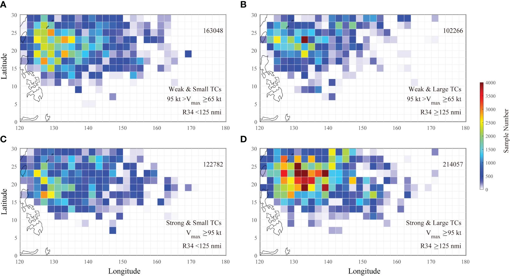
Figure 1 The drifter number distribution of (A) weak small TCs (95 kt > Vmax >64 kt and R34<125 nmi), (B) weak large TCs (95 kt >Vmax >64 kt and R34 ≥125 nmi), (C) strong small TCs (V_max ≥95 kt and R34<125 nmi), and (D) strong large TCs (V_max ≥95 kt and R34 ≥125 nmi).

3 Results

3.1 SST response

Figure 2 shows the SST response induced by four TCs with different intensities and R34s. TC Nida at 1200 UTC, November 24, 2009 (Figure 2A), and TC Omais at 1200 UTC, August 6, 2016 (Figure 2D), were both typhoon category; however, their R34s were quite different, being 57.5 nmi and 270.0 nmi, respectively. The smaller TC Nida caused the strongest SST cooling of −1.6°C, while the larger TC Omais caused the strongest cooling of −3.6°C, with the most intense cooling centered at the right side of the track. In addition to the amplitude, the larger TC caused a wider extent of cooling. A similar phenomenon can also be seen in the cooling of SST induced by strong TC Fengshen at 1200 UTC, 13 July, 2002 (Figure 2C), and TC Mangkhut at 1200 UTC, 14 September, 2018 (Figure 2D). The intensity and R34 of these two TCs were 135 kt with 95.0 nmi and 150 kt with 250.0 nmi, and SST was cooled by up to 2.9°C and 0.9°C, respectively. It is worth noting that for TCs of typhoon category and above, stronger intensity does not lead to stronger SST cooling when R34 is comparable, and intensity no longer has a significant effect on surface ocean response, e.g., although the intensity of TC Fengshen was 135 kt, it induced an SST cooling of less than 1°C, which was much weaker than the cooling caused by TC Omais. Furthermore, when R34 is different but comparable in intensity, the SST response is significantly different in amplitude and extent, e.g., although the intensity of TC Omais (Figure 2B) was weaker than TC Fengshen (Figure 2C) and TC Mangkhut (Figure 2D), it caused the strongest cooling, suggesting that R34 may have a significant effect on ocean responses to TCs.

Figure 2

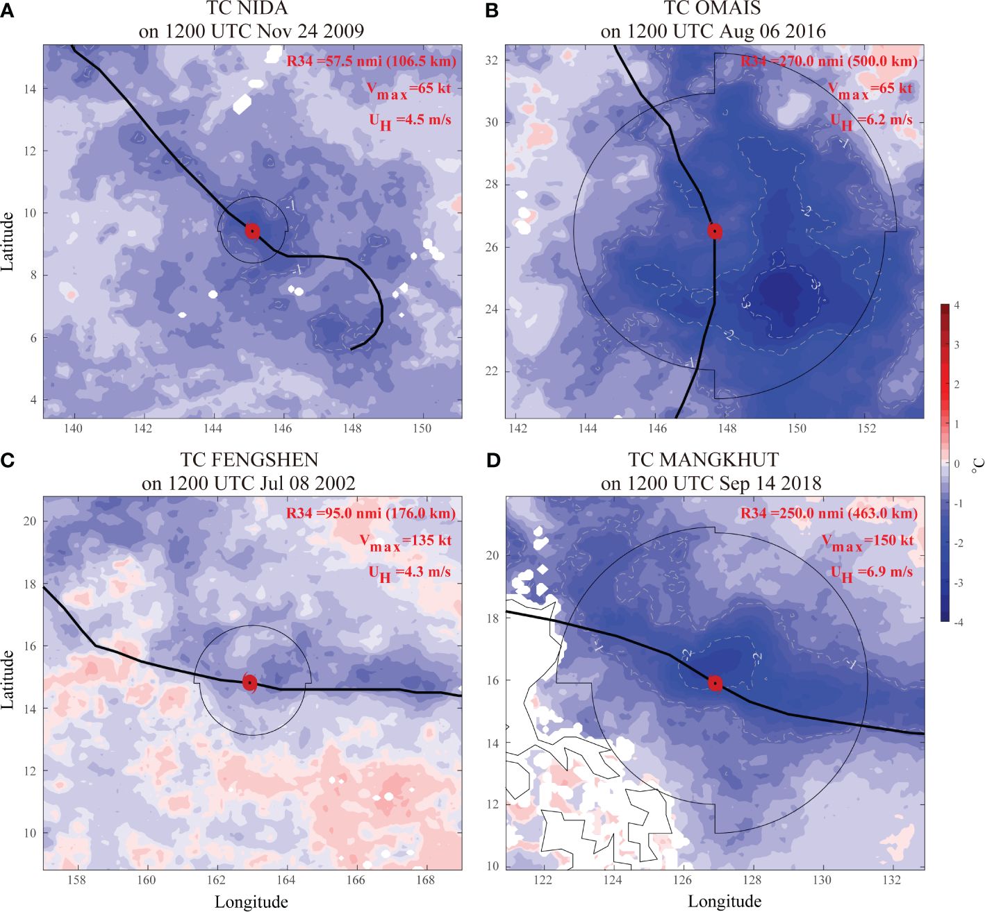
Figure 2 SST cooling of (A) TC Nida at 1200 UTC, 24 November, 2009, (B) TC Omais at 1200 UTC, 6 August, 2016, (C) TC Fengshen at 1200 UTC, 8 July, 2002, and (D) TC Mangkhut at 1200 UTC, 14 September, 2018. SST cooling was calculated as the mean SST 3 days after the TC passage (t_0day to t_3day) minus the mean SST for 3 to 10 days before (t_-10day to t_-3day) the passage. The thin black line represents the extent of R34 at each quadrant. The thin gray dashed lines are the cooling isotherm at −1°C intervals. R34, intensity, and translation speed of each TC are shown the top right corners of each panel.

The fact that TCs with a large R34 cause a larger amplitude and extent of SST cooling can also be seen in statistical analysis. Figures 3A, B show the cross-track profiles of SST responses caused by different intensities and outer sizes of TCs. Both weak (Figure 3A) and strong (Figure 3B) TCs with a large R34 (red error bars) caused stronger SST cooling. Weak small and weak large TCs generated average maximum SST cooling of −1.0°C and −1.9°C, and strong small and strong large TCs cooled down by −1.1°C and −2.0°C around the TC center. The strong TCs cooled 0.1°C more than the weak TCs, and the large TCs cooled 0.9°C more than the small TCs. The difference in SST cooling due to R34 was larger than that due to intensity, which indicates that the SST cooling is more sensitive to TC outer size. The maximum sea surface cooling was located approximately 0.4° to the right side of the TC track. Generally, the SST response is stronger on the right side than on the left side. For small and large TCs, the cooling difference between the two sides is 0.19°C and 0.37°C, respectively, with a maximum temperature difference in the range of 1° -2°from the center of the TCs. The rightward bias distribution is consistent with previous finding (Price et al., 1994; Vincent et al., 2012a; Mei and Pasquero, 2013). There is no significant difference between the asymmetry between TCs with a larger or smaller R34, suggesting that R34 does not affect the asymmetric features (Liu et al., 2023).

Figure 3

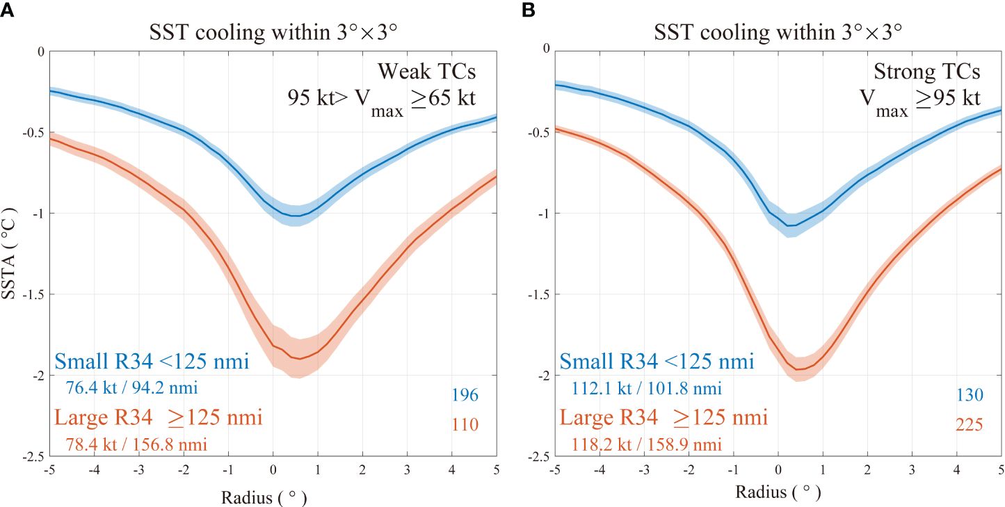
Figure 3 (A) SST cooling radial profile of TCs with small R34s (blue error bars) and large R34s (red error bars) on the cross-track distance of an annulus 0.2° with 95 kt >V_max >64 kt. The error bars indicate standard error. Sample sizes are shown in the bottom right corners. Mean V_max and mean R34 of each group are labeled in the bottom left corners. (B) Same as (A) but for TCs with V_max ≥95 kt.

The dependence of SST cooling on TC intensity and R34 was investigated in Figure 4. TCs with different intensities vary greatly in size.Weak TCs vary in R34 from 40 nmi to 240 nmi, and strong TCs vary from approximately 100 nmi to 200 nmi. Weak TCs can be large and strong TCs can be small. In general, TCs generated more intense SST cooling when R34s were approximately larger than 140 nmi, regardless of TC intensity. A weak TC is capable of causing strong SST cooling if its R34 is large; an intense TC will cause weak SST cooling if its R34 is small. The results in Figures 3, 4 imply that R34 is an important factor and even more influential than TC intensity on the surface ocean response.

Figure 4

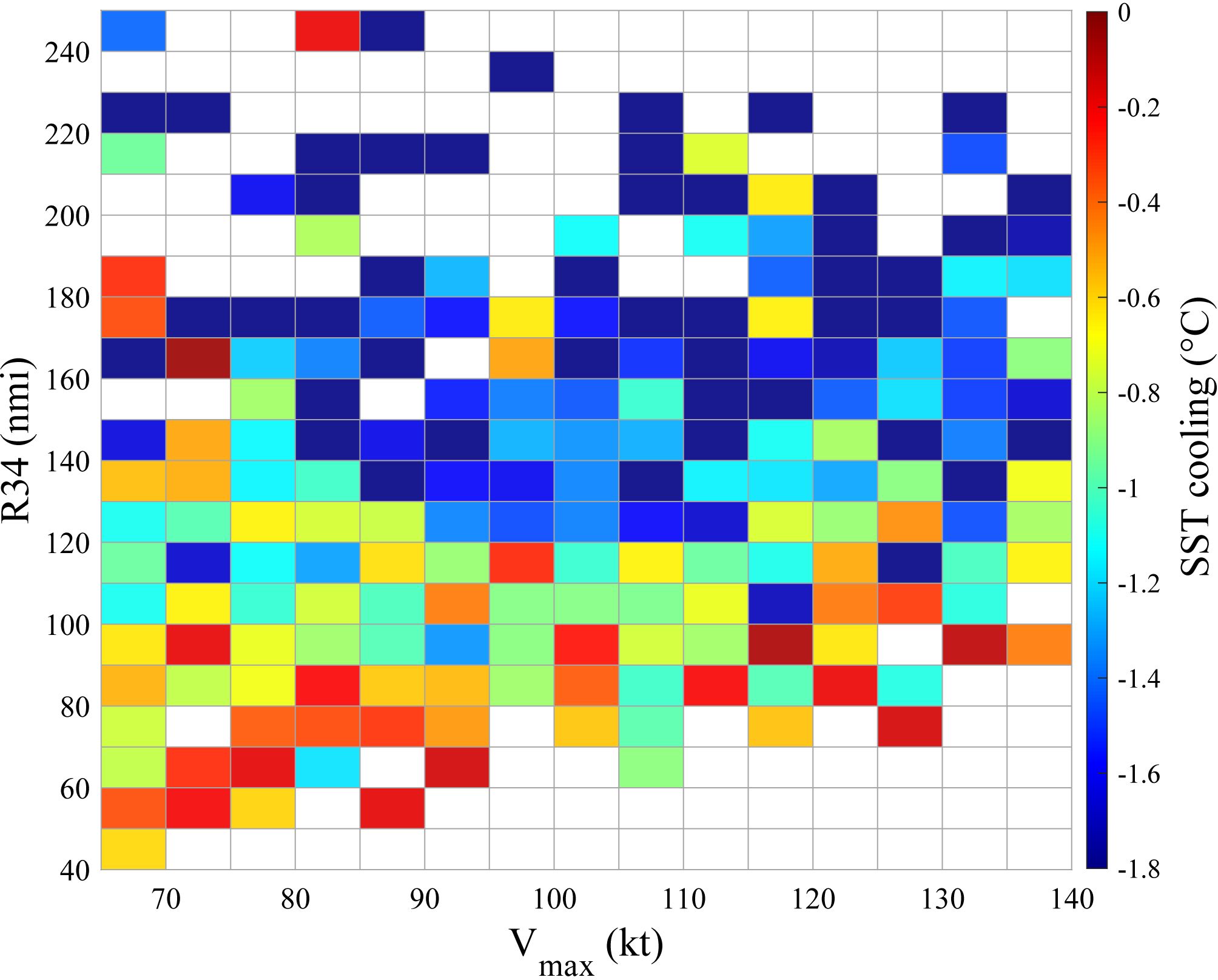
Figure 4 The dependence of SST cooling on TC intensity and R34. SST cooling is defined as the mean SST anomaly within 3° $\times$ 3° boxes with the center of the TC.

3.2 Current response

The change in SST is mainly due to the mixing of the upper ocean caused by TC-induced currents. The radial profile of TC-induced currents is presented in Figures 5A, B. There was an obvious asymmetry in the current response, with the right side having stronger current speed than the left side, which was consistent with the SST response. The difference in current speed induced by large and small TCs was mainly distributed on the right side. Figures 5C, D show the time series of mean current speed, and the x-axis is normalized by the local near-inertial period. The amplitude of current speed increased rapidly when TCs arrived. It increased to 0.80 m/s and 0.88 m/s for small weak and strong TCs, and to 0.95 m/s and 1.0 m/s for weak and strong but large TCs, respectively, with large TCs intensifying more stronger currents than small TCs. The arrows were calculated using the mean zonal and mean meridional current velocity. The clockwise rotation of the currents together with the current speed show a period that coincides with the local near-inertial period, implying that the currents are predominantly near-inertial currents.

Figure 5

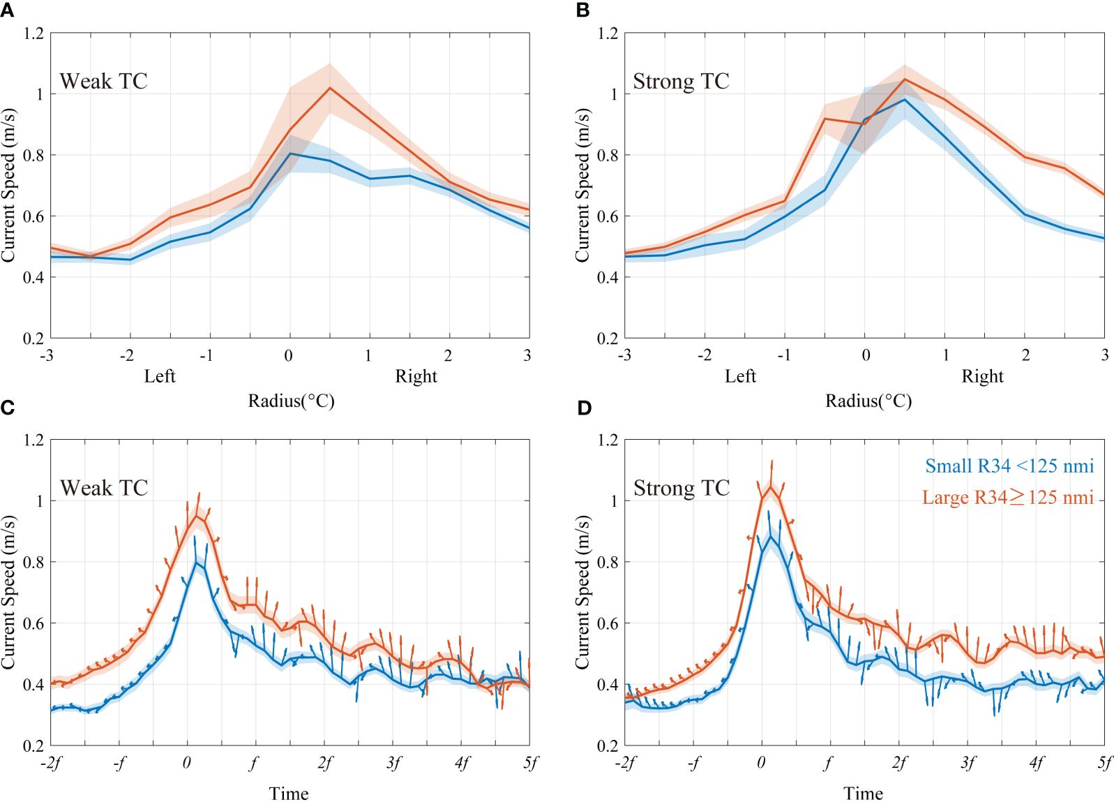
Figure 5 (A) Radial profile of mean currents induced by weak TCs during t₀ to t₃ with small R34s (blue error bars) and large R34s (red error bars) of an annulus 0.5°. (B) Same as (A) but for strong TCs. (C) The time series of mean currents within 3° $\times$ 3°for weak TCs. The x-axis is normalized by the local near-inertial period. Arrows show the direction of currents. (D) Same as (C) but for strong TCs.

As Figures 5C, D show that the currents induced by TCs have a pronounced near-inertial period, we filtered the currents to obtain the time series of near-inertial kinetic energy $E_f$; the results are shown in Figures 6A, B. Similar to the current response, the intensity of the near-inertial currents was comparable for the four groups before the arrival of the TC. This is consistent with previous findings that TCs generate large inertial currents (Geisler, 1970; Pollard, 1970; Large and Crawford, 1995; Guan et al., 2014). The near-inertial kinetic energy $E_f$ of the large weak and strong TCs were 134.8 $J/m^3$ and 126.6 $J/m^3$, respectively, which were significantly higher than those of the small weak and strong TCs of 99.5 $J/m^3$ and 109.1 $J/m^3$. Larger TCs can induce stronger near-inertial kinetic energy, which is consistent with the SST response demonstrated in Figure 3. The effect of size on $E_f$ was more significant than the intensity of the TCs.

Figure 6

Figure 6 The time series of mean near-inertial kinetic energy $E_f$ for (A) weak and (B) strong TCs.

3.3 Non-dimensional analysis

Previous studies have shown the importance of $U_H$ in ocean response (Geisler, 1970; Samson et al., 2009; Mei et al., 2015; Zhang et al., 2020); therefore, we analyzed the non-dimensional Mach number $C$ of each group, and the results are shown in Figure 7. Significance tests did not show significant differences in $C$ between groups, suggesting that the differences in SST and near-inertial current responses were not caused by the $U_H$ of TCs. The Mach number $C$ of all four groups was larger than 2. According to the definition in Greatbatch (1984), it is a fast-moving TC if $C^2\gg 1$; thus, the ocean response to the four groups of TCs is dominated by the inertial wake, which supports with the results presented in Figures 5, 6. The faster the TC moves, the more asymmetric the ocean response (Geisler, 1970). There was no significant difference in the translation speeds, which explains the similar asymmetry of the SST response of the four groups of TCs (Figure 3).

Figure 7

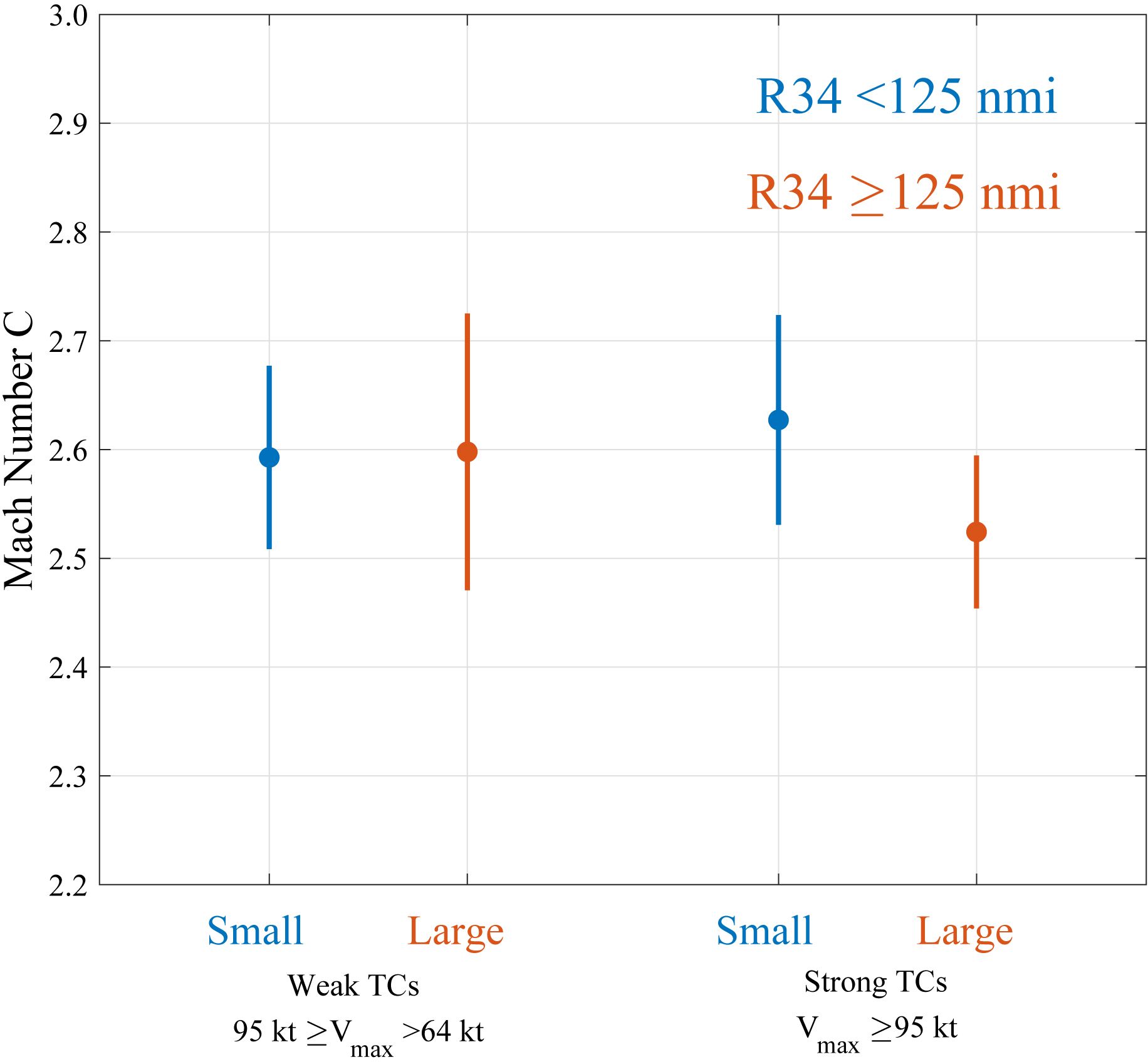
Figure 7 The Mach number of four groups of TCs.

The amplitude of the wake depends on the time of the TC wind field acting on the ocean (Geisler, 1970), also known as the residence time (Price et al., 1994). The translation speed $U_H$ and the scale L will affect the residence time of a TC, and their relationship with SST cooling is shown in Figure 8A. The x-axis is $U_H$, and the y-axis is $2\cdot R34$. Results show that SST cooling is closely related to the ratio of $2\cdot R34$ and $U_H$, which is the residence time $\frac{2\cdot R34}{U_H}$.

Figure 8

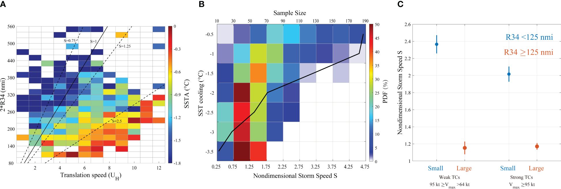
Figure 8 (A) Mean SST cooling within 3° $\times$ 3° around the center as a function of TC translation speed and R34. The thick black line is $S=1$. The three black dashed lines represent $S=0.75$, $S=1.25$, and $S=2.5$. (B) The shading represents the PDFs of $S$ corresponding to different SSTs. The thick black line represents the sample sizes for each SST cooling interval. (C) The non-dimensional storm speed $S$ of four groups of TCs.

The slope of thick black line is the average local near-inertial period $\frac{2\pi }{f}$ (units: s) according to the mean latitude of the TCs. The samples near the thick black line have a residence time comparable with the near-inertial period, i.e., the non-dimensional storm speed $S=\frac{\pi \cdot U_H}{R34\cdot f}$ is approximately 1; the other three black dashed lines are $S=0.75$, $S=1.25$ and $S=2.5$. Samples with $S$ less than 1 have quite strong SST cooling, which could be due to the fact that the TC with $\text{S}<1$ is usually slow moving (defined as moving speeds exceeding 4 m/s; Price, 1981). The response of the ocean to a slow-moving TC also needs to take into account TC-induced upwelling, which contributes 20% to 62% of sea surface cooling (Geisler, 1970; Price, 1981; Chiang et al., 2011). For the fast-moving TCs, which make up 78% of the total sample, their residence time is shorter than the local near-inertial period. Approximately 88.7% of the fast-moving TCs have a residence time shorter than the local near-inertial period, and 71.6% have a resident time shorter than 0.8 times the local near-inertial period; thus, the TCs with larger sizes or slower translation speeds will have longer residence times, which will be closer to the local near-inertial period. Figure 8B shows the probability density function (PDF) of $S$ corresponding to different SSTs, and the results show that the $S$ of the samples cooled by more than 1.5°C was mainly distributed in the range of 0.75 to 1.25, i.e., the residence times of TCs that cause strong SST cooling are approximately equal to the local near-inertial period. The statistics of the four groups of $S$ are displayed in Figure 8C. $S$ was close to 1 for TCs with a large R34 (approximately 1.2 for weak and intense TCs), which was much smaller than that for TCs with a small R34 (2.4 for weak and 2.0 for intense TCs). As there was no significant difference in the Mach number $C$ among the four groups (Figure 7), the value of $S$ was mainly influenced by R34 rather than the $U_H$. The TCs with a larger R34 had a wider outer wind field and therefore the longer residence times were much closer to the local near-inertial period, which is conducive to generating stronger SST cooling. The non-dimensional storm speed $S$ was independent of TC intensity, which explains why the stronger TCs in Figure 3 did not lead to stronger SST cooling if their R34 was the same.

4 Discussion

Previous studies have generally used the Wind Power index (WPi) to explain the amplitude of SST cooling induced by TCs (Vincent et al., 2012a; Liu et al., 2023). The calculation of WPi is based on the power dissipation (Emanuel, 2005), which is defined as ${\displaystyle {\int }_{t_0}^{t_1}\rho C_D{\left|V\right|}^{3}dt}$, where $\rho$ is the surface air density, $C_D$ is the surface drag coefficient, $\left|V\right|$ is the magnitude of the TC wind, $t_0$ is the start and $t_1$ is the end of wind influencing time. WPi takes intensity and the residence time of TCs into account. The residence time is affected by the translation speed and size of TCs, and their effect on SST cooling varies from study to study. Model results showed that a larger size is equivalent to a slower translation speed in terms of SST cooling (Mei et al., 2015). Vincent et al. (2012a) only considered the translation speed and found the linear relationship between WPi and mean SST anomaly. Liu et al. (2023) calculated WPi considering both the translation speed and size and found that Wpi is connected with SST cooling, and the effect of size on ocean response is more profound than translation speed. However, as can be seen from the cases in Figure 2, and the statistical analysis in Figures 3, 4, at least for the samples studied in this paper that have TCs with V_max >64 kt, intensity is no longer the main factor affecting ocean surface response, which cannot be explained by Wpi, as Wpi is closely correlated with TC intensity.

Figure 9 schematically illustrates the interaction time of TCs with different outer sizes. The residence time of a TC is also the frequency of the wind field, which is dominated by the TC outer wind field extent, not to TC intensity. When TCs move at similar translation speeds, the residence times of both weak TCs (dashed lines in Figures 9B, D) and strong TCs (solid lines in Figures 9B, D) are the same if they have the same R34s. Although stronger TCs generally tend to have larger outer sizes (Knaff et al., 2014), TC intensity and outer size are weakly correlated (Merrill, 1984); this may be the reason why some observational studies found that stronger TCs induced stronger SST cooling and also noted a non-monotonic SST response to TC intensity (Lloyd and Vecchi, 2011). According to the results in Figure 8C, the residence time of TCs is typically shorter than the local near-inertial period; the longer residence time of the TCs with a larger R34 will be closer to the local near-inertial period, and thus $S$ will be closer to 1, i.e., the frequency of the wind filed is close to that of the near-inertial oscillation. This would lead to a stronger resonance between the TC wind field and ocean currents and thus trigger stronger upper-ocean vertical mixing, resulting in more intense SST cooling (Price, 1981; Samson et al., 2009). For the samples studied in this paper that have TCs with V_max >64 kt, the effect of R34 is more influential on the SST response than their intensity. The residence time is certainly affected by $U_H$, which is also shown in Figure 8C, but this is not the focus of this study.

Figure 9

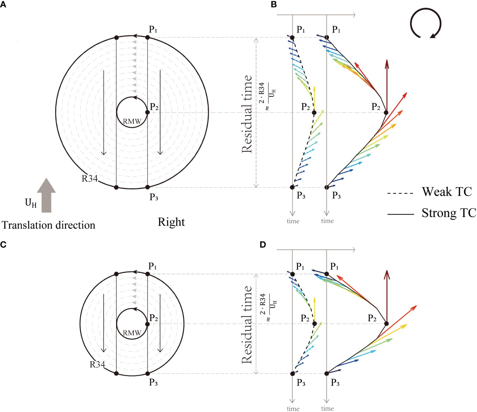
Figure 9 A schematic illustration of the wind fields of a large (A, B) and small (C, D) TC translating from P₁ to P₂ to P₃ on the right side at a speed $U_H$ in the Northern Hemisphere. The distance between P₁ and P₃ is approximately $2\cdot R34$, and the residence time is approximately $\frac{2\cdot R34}{U_H}$.

In addition to the frequency, the rotation of the TC’s wind stress is also considered to be an important factor that influences the resonance. The change rate of wind stress direction of a TC is time and location dependent. For the case from P1 to P3 shown in Figures 9A, C, there is a sudden change in the wind direction just before and after passing through the center of the TC, such as the fastest change in wind direction around P2, and a slow change in wind direction for the rest of the time affected by the TCs’ wind fields, such as the period between P1 to P2 and P2 to P3. In general, the wind field rotates counterclockwise on the left side and clockwise on the right side of the TCs’ tracks. The clockwise rotation on the right side accelerates the inertial ocean currents, resulting in stronger inertial oscillations, SST cooling, and current responses (Price, 1981; Dickey and Simpson, 1983; Skyllingstad et al., 2000; Stockwell et al., 2004; Chen et al., 2015), which explains the asymmetry in the SST and current responses observed in this study.

Finally, we discuss the optimality of R34. The statistics revealed that SST cooling is more sensitive to R34 and has the best correlation coefficient compared with other wind radii (Liu et al., 2023). The scale $L$ in $S$ has usually replaced or been estimated by RMW in previous studies, and the formulation of $S$ differs from study to study, such as $S=\frac{U_H}{2RMWf}$ in Price (1983) and D’Asaro et al. (2014), $S=\frac{\pi U_H}{4fRMW}$ in Price et al. (1994), $S=\frac{\pi U_H}{2fRMW}$ in Samson et al. (2009), and $S=\frac{U_H}{fRMW}$ in Zhang et al. (2020) and Zhang (2023). Based on Simpson and Dickey (1981), the ocean response is wind-dominated when the 10-m wind speed exceeds 10 m/s. Wind speeds near the RMW of TCs are generally larger than this threshold, and the RMW usually contracts to less than 30 nmi and stays constant when TC intensity is stronger than 60 kt (Wu and Ruan, 2021). These characteristics of the RMW imply that there may be a large error in estimating the residence time of a TC when using the RMW to represent the scale $L$ in $S$. The size information of a TC in the JTWC includes the RMW, R64, R50, and R34, in which 34kt is the closest to the threshold 10 m/s ($\approx$ 19.4 kt) in Simpson and Dickey (1981). It has been tested that the correlation coefficients between $S$ and the mean SST anomaly within 3° $\times$ 3° when using the RMW, R64, R50, and R34 are −0.19, −0.40, −0.43, and −0.46, respectively, which also demonstrates the optimality of using R34 in the definition of scale L $SL$.

5 Conclusions

We analyzed ocean responses to TC intensity and outer size in the Northwest Pacific in this study using satellite and drifter data. The results show that for samples for which TC intensity is stronger than typhoon category, SST cooling is stronger when TC outer size is larger ($\approx$ R34 >140 nmi) for strong (V_max ≥95 kt) and weak (95 kt >V_max >64 kt) TCs. Strong TCs induced 0.1°C more SST cooling than weak TCs, and large TCs (R34 ≥125 nmi) induced 0.9°C more SST cooling than small TCs (R34<125 nmi). Thus, SST response is more sensitive to TC outer size than to TC intensity. Drifter data show that TCs generate strong currents with near-inertial periods, and that larger TCs will generate more intense currents. Near-inertial kinetic energy $E_f$ was calculated from the near-inertial current $u_f$ and $v_f$ after bandpass filtering of the ocean current, and the results showed that TCs with a larger R34 will trigger stronger $E_f$.

Non-dimensional analysis suggested that the non-dimensional storm speed $S$ for large TCs is close to 1. In most conditions, the residence time of a TC is shorter than the local inertial period. The residence time depends on TC outer size and $U_H$, not TC intensity. Therefore, when $U_H$ values are comparable, a larger TC that has a larger outer wind field extent will have a longer residence time, which will be closer to the near-inertial oscillation period, and can lead to the resonance of the TC wind field with ocean currents (Price, 1981; Dickey and Simpson, 1983; Price et al., 1994; Samson et al., 2009) and ultimately lead to stronger SST cooling and currents. Our analysis demonstrates the importance of TC outer size in the ocean response and emphasizes that TC outer size is not negligible in the study of sea-air interaction processes.

Data availability statement

The datasets presented in this study can be found in online repositories. The names of the repository/repositories and accession number(s) can be found below: https://www.metoc.navy.mil/jtwc/jtwc.html?western-pacific; https://data.remss.com/SST/daily/mw_ir/v05.1/; https://www.aoml.noaa.gov/ftp/phod/buoydata/hourly_product/v1.04/.

Author contributions

ZR: Conceptualization, Writing – original draft, Writing – review & editing, Data curation, Formal analysis, Investigation, Methodology, Software, Validation, Visualization. BL: Conceptualization, Funding acquisition, Writing – review & editing. CY: Conceptualization, Methodology, Writing – review & editing. RD: Conceptualization, Writing – review & editing. PB: Funding acquisition, Writing – review & editing. QW: Methodology, Writing – review & editing.

Funding

The author(s) declare financial support was received for the research, authorship, and/or publication of this article. This study was funded by the National Key Research and Development Program of China (2023YFD2401901), the National Natural Science Foundation of China (42106017), the Special Fund for Zhejiang Ocean University from the Bureau of Science and Technology of Zhoushan (2023C41006) and the National Natural Science Foundation of China (41706022).

Conflict of interest

The authors declare that the research was conducted in the absence of any commercial or financial relationships that could be construed as a potential conflict of interest.

Publisher’s note

All claims expressed in this article are solely those of the authors and do not necessarily represent those of their affiliated organizations, or those of the publisher, the editors and the reviewers. Any product that may be evaluated in this article, or claim that may be made by its manufacturer, is not guaranteed or endorsed by the publisher.

References

Black W. J., Dickey T. D. (2008). Observations and analyses of upper ocean responses to tropical storms and hurricanes in the vicinity of Bermuda. J. Geophys. Res.: Oceans 113 (8). doi: 10.1029/2007JC004358

CrossRef Full Text | Google Scholar

Chen S., Polton J. A., Hu J., Xing J. (2015). Local inertial oscillations in the surface ocean generated by time-varying winds. Ocean Dyn. 65, 1633–1641. doi: 10.1007/s10236-015-0899-6

CrossRef Full Text | Google Scholar

Chiang T. L., Wu C. R., Oey L. Y. (2011). Typhoon Kai-Tak: An ocean’s perfect storm. J. Phys. Oceanogr. 41, 221–233. doi: 10.1175/2010JPO4518.1

CrossRef Full Text | Google Scholar

Cui H., Tang D., Mei W., Liu H., Sui Y., Gu X. (2023). Predicting tropical cyclone-induced sea surface temperature responses using machine learning. Geophys. Res. Lett. 50 (18), 1–11. doi: 10.1029/2023GL104171

CrossRef Full Text | Google Scholar

D’Asaro E., Black P., Centurioni L., Harr P., Jayne S., Lin I. I., et al. (2011). Typhoon-ocean interaction in the western North Pacific: Part 1. Oceanogr. 24 (4), 24–31. doi: 10.5670/oceanog.2011.91

CrossRef Full Text | Google Scholar

D’Asaro E. A., Black P. G., Centurioni L. R., Chang Y. T., Chen S. S., Foster R. C., et al. (2014). Impact of typhoons on the ocean in the pacific. Bull. Am. Meteorol. Soc. 95, 1405–1418. doi: 10.1175/BAMS-D-12-00104.1

CrossRef Full Text | Google Scholar

D’Asaro E. A., Sanford T. B., Niiler P. P., Terrill E. J. (2007). Cold wake of hurricane Frances. Geophys. Res. Lett. 34, 2–7. doi: 10.1029/2007GL030160

CrossRef Full Text | Google Scholar

Dickey T. D., Simpson J. J. (1983). The influence of optical water type on the diurnal response of the upper ocean. Tellus B 35 B, 142–154. doi: 10.1111/j.1600-0889.1983.tb00018.x

CrossRef Full Text | Google Scholar

Elipot S., Lumpkin R., Perez R. C., Lilly J. M., Early J. J., Sykulski A. M. (2016). A global surface drifter data set at hourly resolution. J. Geophys. Res.: Oceans 121, 2937–2966. doi: 10.1002/2016JC011716

CrossRef Full Text | Google Scholar

Emanuel K. (2003). Tropical cyclones. Annu. Rev. Earth Planet. Sci. 31, 75–104. doi: 10.1146/annurev.earth.31.100901.141259

CrossRef Full Text | Google Scholar

Emanuel K. (2005). Increasing destructiveness of tropical cyclones over the past 30 years. Nature 436, 686–688. doi: 10.1038/nature03906

PubMed Abstract | CrossRef Full Text | Google Scholar

Geisler J. E. (1970). Linear theory of the response of a two layer ocean to a moving hurricane‡. Geophys. Fluid Dyn. 1, 249–272. doi: 10.1080/03091927009365774

CrossRef Full Text | Google Scholar

Greatbatch R. J. (1984). On the response of the ocean to a moving storm: Parameters and scales. J. Phys. Oceanogr. 14, 59–78. doi: 10.1175/1520-0485(1984)014<0059:OTROTO>2.0.CO;2

CrossRef Full Text | Google Scholar

Guan S., Jin F. F., Tian J., Lin I. I., Pun I. F., Zhao W., et al. (2024). Ocean internal tides suppress tropical cyclones in the South China Sea. Nat. Commun. 15, 1–12. doi: 10.1038/s41467-024-48003-y

PubMed Abstract | CrossRef Full Text | Google Scholar

Guan S., Zhao W., Huthnance J., Tian J., Wang J. (2014). Observed upper ocean response to typhoon Megi, (2010) in the Northern South China Sea. J. Geophys. Res.: Oceans 119, 3134–3157. doi: 10.1002/2013JC009661

CrossRef Full Text | Google Scholar

Haakman K., Sayol J. M., van der Boog C. G., Katsman C. A. (2019). Statistical characterization of the observed cold wake induced by North Atlantic hurricanes. Remote Sens. 11 (20), 2368. doi: 10.3390/rs11202368

CrossRef Full Text | Google Scholar

Knaff J. A., Longmore S. P., Molenar D. A. (2014). An objective satellite-based tropical cyclone size climatology. J. Climate 27, 455–476. doi: 10.1175/JCLI-D-13-00096.1

CrossRef Full Text | Google Scholar

Large W. G., Crawford G. B. (1995). Observations and simula- tions of upper ocean response to wind events during the Ocean Storms Experiment. J. Phys. Oceanogr. 25, 2831–2852.

Google Scholar

Liu Y., Guan S., Lin I. I., Mei W., Jin F. F., Huang M., et al. (2023). Effect of storm size on sea surface cooling and tropical cyclone intensification in the western north Pacific. J. Climate 36, 7277–7296.

Google Scholar

Lloyd I. D., Vecchi G. A. (2011). Observational evidence for oceanic controls on hurricane intensity. J. Climate 24, 1138–1153. doi: 10.1175/2010JCLI3763.1

CrossRef Full Text | Google Scholar

Mao Q., Chang S. W., Pfeffer R. L. (2000). Influence of large-scale initial oceanic mixed layer depth on tropical cyclones. Monthly Weather Rev. 128, 4058–4070. doi: 10.1175/1520-0493(2000)129<4058:IOLSIO>2.0.CO;2

CrossRef Full Text | Google Scholar

Mei W., Lien C. C., Lin I. I., Xie S. P. (2015). Tropical cyclone-induced ocean response: A comparative study of the south China sea and tropical northwest Pacific. J. Climate 28, 5952–5968. doi: 10.1175/JCLI-D-14-00651.1

CrossRef Full Text | Google Scholar

Mei W., Pasquero C. (2013). Spatial and temporal characterization of sea surface temperature response to tropical cyclones. J. Climate 26, 3745–3765. doi: 10.1175/JCLI-D-12-00125.1

CrossRef Full Text | Google Scholar

Merrill R. T. (1984). A comparison of large and small tropical cyclones. Monthly Weather Rev. 112, 1408–1418. doi: 10.1175/1520-0493(1984)112<1408:ACOLAS>2.0.CO;2

CrossRef Full Text | Google Scholar

Pollard R. T. (1970). On the generation by winds of inertial waves in the ocean. Deep-Sea Res. Oceanographic Abstracts 17, 795–812. doi: 10.1016/0011-7471(70)90042-2

CrossRef Full Text | Google Scholar

Price J. F. (1981). Upper ocean response to a hurricane. J. Phys. Oceanogr. 11, 153–175. doi: 10.1175/1520-0485(1981)011<0153:UORTAH>2.0.CO;2

CrossRef Full Text | Google Scholar

Price J. F. (1983). Internal wave wake of a moving storm. Part I. Scales, energy budget and observations. J. Phys. Oceanogr. 13, 949–965. doi: 10.1175/1520-0485(1983)013<0949:IWWOAM>2.0.CO;2

CrossRef Full Text | Google Scholar

Price J. F., Sanford T. B., Forristall G. Z. (1994). Forced stage response to a moving hurricane. J. Phys. Oceanogr. 24, 233–260. doi: 10.1175/1520-0485(1994)024<0233:FSRTAM>2.0.CO;2

CrossRef Full Text | Google Scholar

Pun I. F., Knaff J. A., Sampson C. R. (2021). Uncertainty of tropical cyclone wind radii on sea surface temperature cooling. J. Geophys. Res.: Atmos. 126, 1–19. doi: 10.1029/2021JD034857

CrossRef Full Text | Google Scholar

Pun I. F., Lin I. I., Lien C. C., Wu C. C. (2018). Influence of the size of Supertyphoon Megi, (2010) on SST cooling. Monthly Weather Rev. 146, 661–677. doi: 10.1175/MWR-D-17-0044.1

CrossRef Full Text | Google Scholar

Samson G., Giordani H., Caniaux G., Roux F. (2009). Numerical investigation of an oceanic resonant regime induced by hurricane winds. Ocean Dyn. 59, 565–586. doi: 10.1007/s10236-009-0203-8

CrossRef Full Text | Google Scholar

Shay L. K., Goni G. J., Black P. G. (2000). Effects of a warm oceanic feature on Hurricane Opal. Monthly Weather Rev. 128, 1366–1383. doi: 10.1175/1520-0493(2000)128<1366:EOAWOF>2.0.CO;2

CrossRef Full Text | Google Scholar

Simpson J. J., Dickey T. D. (1981). The relationship between downward irradiance and upper ocean structure. J. Phys. Oceanogr. 11, 309–323. doi: 10.1175/1520-0485(1981)011<0309:TRBDIA>2.0.CO;2

CrossRef Full Text | Google Scholar

Skyllingstad E. D., Smyth W. D., Crawford G. B. (2000). Resonant wind-driven mixing in the ocean boundary layer. J. Phys. Oceanogr. 30, 1866–1890. doi: 10.1175/1520-0485(2000)030<1866:RWDMIT>2.0.CO;2

CrossRef Full Text | Google Scholar

Stockwell R. G., Large W. G., Milliff R. F. (2004). Resonant inertial oscillations in moored buoy ocean surface winds. Tellus A: Dyn. Meteorol. Oceanogr. 56, 536. doi: 10.3402/tellusa.v56i5.14478

CrossRef Full Text | Google Scholar

Sun J., Oey L. Y., Chang R., Xu F., Huang S. M. (2015). Ocean response to typhoon Nuri, (2008) in western Pacific and South China Sea. Ocean Dyn. 65, 735–749. doi: 10.1007/s10236-015-0823-0

CrossRef Full Text | Google Scholar

Vincent E. M., Lengaigne M., Madec G., Vialard J., Samson G., Jourdain N. C., et al. (2012a). Processes setting the characteristics of sea surface cooling induced by tropical cyclones. J. Geophys. Res.: Oceans 117, 1–18. doi: 10.1029/2011JC007396

CrossRef Full Text | Google Scholar

Vincent E. M., Lengaigne M., Vialard J., Madec G., Jourdain N. C., Masson S. (2012b). Assessing the oceanic control on the amplitude of sea surface cooling induced by tropical cyclones. J. Geophys. Res.: Oceans 117, 1–14. doi: 10.1029/2011JC007705

CrossRef Full Text | Google Scholar

Wu Q., Ruan Z. (2021). Rapid contraction of the radius of maximum tangential wind and rapid intensification of a tropical cyclone. J. Geophys. Res.: Atmos. 126, 1–15. doi: 10.1029/2020JD033681

CrossRef Full Text | Google Scholar

Wu R., Li C. (2018). Upper ocean response to the passage of two sequential typhoons. Deep Sea Res. Part I: Oceanographic Res. Papers 132, 68–79. doi: 10.1016/j.dsr.2017.12.006

CrossRef Full Text | Google Scholar

Yablonsky R. M., Ginis I. (2009). Limitation of one-dimensional ocean models for coupled hurricane–ocean model forecasts. Monthly Weather Rev. 137, 4410–4419. doi: 10.1175/2009MWR2863.1

CrossRef Full Text | Google Scholar

Zedler S. E. (2009). Simulations of the ocean response to a hurricane: Nonlinear processes. J. Phys. Oceanogr. 39, 2618–2634. doi: 10.1175/2009JPO4062.1

CrossRef Full Text | Google Scholar

Zhang H. (2023). Modulation of upper ocean vertical temperature structure and heat content by a fast-moving tropical cyclone. J. Phys. Oceanogr. 53, 493–508. doi: 10.1175/JPO-D-22-0132.1

CrossRef Full Text | Google Scholar

Zhang H., Liu X., Wu R., Chen D., Zhang D., Shang X., et al. (2020). Sea surface current response patterns to tropical cyclones. J. Mar. Syst. 208, 103345. doi: 10.1016/j.jmarsys.2020.103345

CrossRef Full Text | Google Scholar

Zhang J., Lin Y., Chavas D. R., Mei W. (2019). Tropical cyclone cold wake size and its applications to power dissipation and ocean heat uptake estimates. Geophysical Res. Lett. 46, 10177–10185. doi: 10.1029/2019GL083783

CrossRef Full Text | Google Scholar