Assessment of daily altimeter-based open ocean water level with hindcast and forecast efficiency

Satellite altimetry water level measurements are valuable in episodic and climate change related hydrodynamic impact studies, despite their sparse temporal distribution over the global ocean. This study presents the spatiotemporal characteristics of the open-ocean satellite derived water level measurements globally for the period 31/12/1992-15/10/2019 and evaluates their efficacy to represent the water level even during intense atmospheric conditions. Water level measurements from 23 different satellite missions are compared with tide gauge records and hydrodynamic simulations. The satellite measurements reproduce the water-level variations with good to excellent skill for ~60% of the areas considered. Additionally, satellite measurements and local atmospheric conditions are utilized in order to examine whether statistical data driven models can contribute to decreasing the temporal sparseness of the water level data over the global ocean. The suitability of this low computational-cost method is demonstrated by deriving a 63-year hindcast of the daily maximum water level for the global ocean, and for a medium-term 15-day ensemble forecast. The publicly available long-term water-level hindcast and the parameters of the data-driven statistical model derived can serve as a tool for designing and facilitating local and global coastal risk-assessment studies.

1 Introduction

For early warning, predicting extreme water level (WL) events in deep water, storm surge and coastal flood levels before they happen is still the holy grail of oceanic research. Well-benchmarked global coupled models are essential for accurate predictions over large spatial and temporal scales, yet the incredibly varied distribution of winds, currents and temperatures over orders of magnitude differences in oceanic depths and atmospheric heights make any high-resolution estimates on the sea surface a vexing and complex numerical undertaking, begging the question of how to best use sparse satellite measurements to improve hindcasting and forecasting.

Water level measurements are important in understanding the hydrodynamic conditions along the global ocean. WL measurements can be obtained in situ with tide gauges (TG) (Woodworth et al., 2016), offshore buoys, seismometers (Okal, 2021), amateur videos (Fritz et al., 2006), mission-oriented cinematography (Holman and Stanley, 2007), and remotely, with satellite altimeters (Ballarotta et al., 2023; Morrow et al., 2023). Each method varies in temporal and spatial resolution, but also in coverage and applicability.

TG high-frequency WL measurements with temporal range of <1-min have been used for detection of rapidly evolving phenomena such as meteotsunamis, tsunamis and seiches (Woodworth et al., 2016). When TG measurements are averaged at lower frequencies, they can be used for the assessment of longer oscillations, such as monthly, seasonal, interannual and Mean Sea Level (MSL) or sea level rise (SLR) studies; TG measurements with short duration up to one month are often used to derive basic local tidal constituents, while decadal scales are necessary to accurately estimate SLR rates (see for instance Burgette et al., 2013; Houston and Dean, 2011; Jevrejeva et al., 2006; Tsimplis and Spencer, 1997).

Additionally, the spatial extent and resolution of the WL measurements is crucial for risk assessments during highly energetic events that may impact the coastal zone. While a dense network of in situ instruments is the golden standard for inferring local hydromorphodynamic conditions, at global scales, satellite altimeters provide the most comprehensive, spatially distributed, but often sparse measurements.

Altimeter measurements have been utilized for the analysis and better understanding of tsunamis (Okal et al., 1999), oceanic winds and wave heights (Timmermans et al., 2020; Wang et al., 2023; Young and Ribal, 2019), in understanding high resolution sea level trends at the coastal zone (Cazenave et al., 2022; Marti et al., 2021; The Climate Change Initiative Coastal Sea Level Team et al., 2020), sea level anomalies (SLA), for intercomparisons of tidal analyses (Valle-Rodríguez and Trasviña-Castro, 2020), estimations of SLR rate up to 20 km from the coast (Cazenave et al., 2022), annual sea-level cycle characterization (Cipollini et al., 2017) and coastal overtopping estimation (Almar et al., 2021). Due to the increasing volume and accuracy of altimeter-derived WL data, several studies advocate the development of consistent multi-mission datasets for the lake WL, river discharges, significant wave heights (Abdalla et al., 2021; Takbash et al., 2019), ocean circulation (Liu et al., 2016) and for coastal applications (Cipollini et al., 2010).

Scharroo et al. (2005) appear to be the first study to infer storm surge levels (SSL) from altimeter-derived WL, as measured by the GEOSAT Follow-on (GFO), ENVISAT (ENVIronmental SATellite), ERS-2, Jason-1 and TOPEX missions. Han et al. (2012) compared the SSL measurements from Jason-2 with TG records during the landfall of hurricane Igor at the Island of Newfoundland, a tropical cyclone which originated in Cape Verde in 2010. Not only they found good agreement, but they were also able to identify the equatorward free continental-shelf wave which caused the maximum surge at St. John and Argentia, Newfoundland during Igor. In this context, Andersen et al. (2015) claimed that they could identify more than 90% of the high water events in the North Sea using data from as few as two altimeter missions.

Han et al. (2017) analyzed the Jason-1 and Jason-2 SLA (without the inverse barometric correction) during Hurricane Isaac’s passage in August 2012 at the Gulf of Mexico and also found good agreement with local TG measurements. Despite only examining a single event, they suggested that effective monitoring of storm surges is possible through an appropriately distributed constellation of satellite altimeters. For the Bay of Bengal, Antony et al. (2014) concluded that ~45% of surge events could be identified by utilizing WL data obtained by the Topex/Poseidon, Jason-1, Geosat Follow-On and ENVISAT missions. Pascual et al. (2006) suggested that the coastal WL is better reproduced by four satellites (Jason-1, ERS-2/ENVISAT, Topex/Poseidon interleaved with Jason-1 and Geosat Follow-On) than by two (Jason-1 + ERS-2/ENVISAT), with a reduced error of ~25%, when compared to TG data. Ji et al. (2019) analyzed multi-satellite altimeter data for China’s coastal area, and found that 26% of the surge events recorded at the TG stations were also measured by the satellite altimeters. Sánchez-Román et al. (2020) assessed the performance of the Level-3 (L3) SLA measurements obtained by Sentinel-3A and Jason-3 with 270 TG records for a period of 2.5 years along the European coastline. They found better agreement between the Sentinel-3A and the TG records compared to Jason-3, and even better agreement when the long-wavelength error (lwe) correction was applied.

In terms of operational monitoring and ocean state forecasting, Pascual et al. (2009) demonstrated the superiority of the delayed time (DT) altimeter observations versus real-time data, and argued that four altimeters are needed in real time to get similar quality performance as two altimeters in DT. Fenoglio-Marc et al. (2015) compared the SARAL/AltiKa along-track SSL during the landfall of cyclone Xaver at the North Sea in 2013, and found good agreement with numerical predictions. Philippart et al. (1998) utilized the ERS-1, ERS-2 and TOPEX/POSEIDON altimeter data and demonstrated that it is possible to calibrate the Dutch Continental Shelf Model, only with altimeter data. They also highlighted that the delivery time of analyzed altimeter data can be a limiting factor for operational storm-surge forecasts. Etala et al. (2015) and De Biasio et al. (2017) reported improved SSL forecasts along the Argentinian coast and the Gulf of Venice, Italy, respectively, by including sparse altimeter data assimilation. On the statistical reconstruction of the long term SSL, Cid et al. (2017) utilized the dynamic atmospheric correction (DAC) in combination with the atmospheric conditions, and they derived the global maximum SSL for the period 1871-2010. Following a similar approach, Ji et al. (2020) constructed the daily maximum SSL for SE China using the SLA and DAC components and the atmospheric conditions and further improved the statistical derived storm surge levels after calibrating it with the TG records.

The Data Unification and Altimeter Combination System (DUACS) has been providing multi-satellite near-real-time (NRT) and DT L3 along-track [https://doi.org/10.48670/moi-00146] and Level-4 (L4) [https://doi.org/10.48670/moi-00144] gridded altimetry data for more than twenty years. It incorporates Level 2P altimetry products provided by space agencies, and aims to provide a consistent and homogenous among-missions SLA dataset (including instrumental, geophysical and environmental corrections with mean sea surface and validity flag) for mesoscale and climate applications (Taburet et al., 2019).

Leveraging these developments, our study is the first global open-ocean WL study utilizing only the publicly available but sparse DT DUACS L3 along-track WL measurements. Our aim is to demonstrate how to use such sparse satellite measurements for both the long term hindcast and real time water-level forecasts. Our presentation is organized as follows. In Section 2, we present the available spatiotemporal characteristics of the DT DUACS L3 along-track WL measurements over the open ocean, as well as the TG and the numerical model we use for validation. Section 3 discusses the validation of the temporal sparse altimeter WL, as well as the continuous WL, as derived from data-driven statistical models, for our reference 27-year period 1993-2019. The last part of Section 3 presents two demonstration cases underscoring the applicability of the satellite measurements for both the hindcasting and the medium range forecasting of oceanic water-level variations, in a computationally cost effective framework. The discussion and our conclusions are presented in Section 4.

2 Materials and methods

2.1 Altimeter water level measurements

This study is based on the DT DUACS L3 along-track altimeter WL measurements obtained from 23 missions, as available at the Copernicus Marine Service (CMEMS) web portal¹ (downloaded on 16/03/2020) covering the period 31/12/1992-15/10/2019 (Supplementary Table S1). Although the CMEMS DT L3 dataset extends until 08/06/2023, we use 27 years of measurements to validate first, and then explore hindcast and forecast capacities.

The dataset describes the along-track global SLA with 1Hz (7 km) spatial resolution with respect to its twenty-year 2012 mean obtained from the Jason-3, Sentinel-3A/B, HY-2A, Saral/AltiKa, Cryosat-2, Jason-2, Jason-1, T/P, ENVISAT, GFO, ERS1/2 missions. To allow correction of the SLA measurements from inherent geophysical and mechanical errors, the dataset includes metadata (Taburet et al., 2019), hence the corrected SLA is estimated as:

$\begin{array}{ll}sl{a}_{cor}=sl{a}_{uncor}-dac-ocea{n}_{tide}+lwe& (1)\end{array}$

where sla_cor is the sea surface height above the MSL during the period 1993-2019, sla_uncor is the uncorrected sea level anomalies (m), dac is the dynamic atmospheric correction component (m), ocean_tide is the ocean, pole and solid earth tidal elevation (m), and finally lwe is the long- wavelength error (m), see Le Traon et al. (2003). The contribution of tides to the WL altimeter measurements is not considered in this study as we aim to evaluate the efficacy of the altimeter measurements to describe the non-deterministic water level variations. The reader is referred to the Supplementary Material for a complete description of the utilized components. In our study, we use the related variables SLAwithDAC, SLAnoDAC and DAC as:

$\begin{array}{ll}SLAwithDAC=sl{a}_{cor}+dac-lwe& (2)\end{array}$

$\begin{array}{ll}SLAnoDAC=sl{a}_{cor}& (3)\end{array}$

$\begin{array}{ll}DAC=dac& (4)\end{array}$

Since the focus of this study is to assess how to use satellite derived hourly, sub-daily and daily maximum WL to analyze highly energetic hydrodynamic events, we use the DT DUACS L3 along-track altimeter WL, which is practically instantaneous, however has far more sparse data compared to the daily temporal resolution DT DUACS L4 gridded SLA data. Additionally, the DT DUACS L4 gridded SLA dataset already includes the DAC atmospheric correction. Moreover, we do not utilize the X-TRACK-L2P SLA [10.24400/527896/a01-2022.020] developed by the Center of Topography of the Ocean and Hydrosphere (CTOH) and the Laboratory of Space Geophysical and Oceanographic Studies (LEGOS) because it is tailored for coastal ocean applications (Birol et al., 2017), while we aim to demonstrate the suitability of deriving the daily maximum WL from satellite measurements in the open ocean.

We note that the starting operating date of the WL measurements (see Supplementary Table S1) may deviate from the starting date in Table 1 of the CMEMS Quality Information Document², reflecting the availability of the data at the CMEMS ftp server on the acquisition date. For the purpose of clarity, the remaining subsection will outline the temporal distribution during the period 31/12/1992-15/10/2019 and the spatial distribution across the global ocean of the available dataset.

The number of measurements throughout the data acquisition period is shown in Supplementary Figure S1. Indicatively, from 1992 to 2000 the number of measurements increases ~45% with the introduction of three concurrent missions (ers2, g2, tpn - see Supplementary Table S1 for a list of mission abbreviation) with a total of ~2.1x107 acquisitions up until 2005. Compared to 2000, a ~16% reduction is observed in 2008 (~1.3x107) followed by an increase in 2011 (~2.1x107) and a decrease in 2012 (~1.6x107). The amount of measurements peaked in 2017 with ~2.8x107 measurements obtained by seven concurrent missions (alg, c2, h2g, j2g, j2n, j3, s3a).

The available along-swath SLAwithDAC, SLAnoDAC and DAC components from all the missions are combined into a 0.25°x0.25° global WGS84 grid to allow us to analyze the temporal characteristics of this dataset. The first step was to remove the land areas defined by the Natural Earth 1:50m v4.0.0 coastline³ (accessed on 15/02/2022). Afterwards, the centroids of the developed grid are used as reference points. For each hourly timestep, we averaged all the available DT DUACS L3 along-track measurements that are located inside and on the margins of each cell defined by the grid centroid -/+0.125°. Indicatively, the maximum WL at each grid node during the period 31/12/1992-15/10/2019 of the three components SLAnoDAC, SLAwithDAC and DAC is presented in Supplementary Figure S2.

The areas without measurements account for ~12.87% of the global ocean surface. They are mostly located north and south of -/+80°, along the coastline of Greenland, Hudson Bay, the east coast of Canada, the north coast of the Scandinavian Peninsula, southern Patagonia, the Weddell Sea, and along the coastline of the east Arctic ocean (Figure 1).

Figure 1

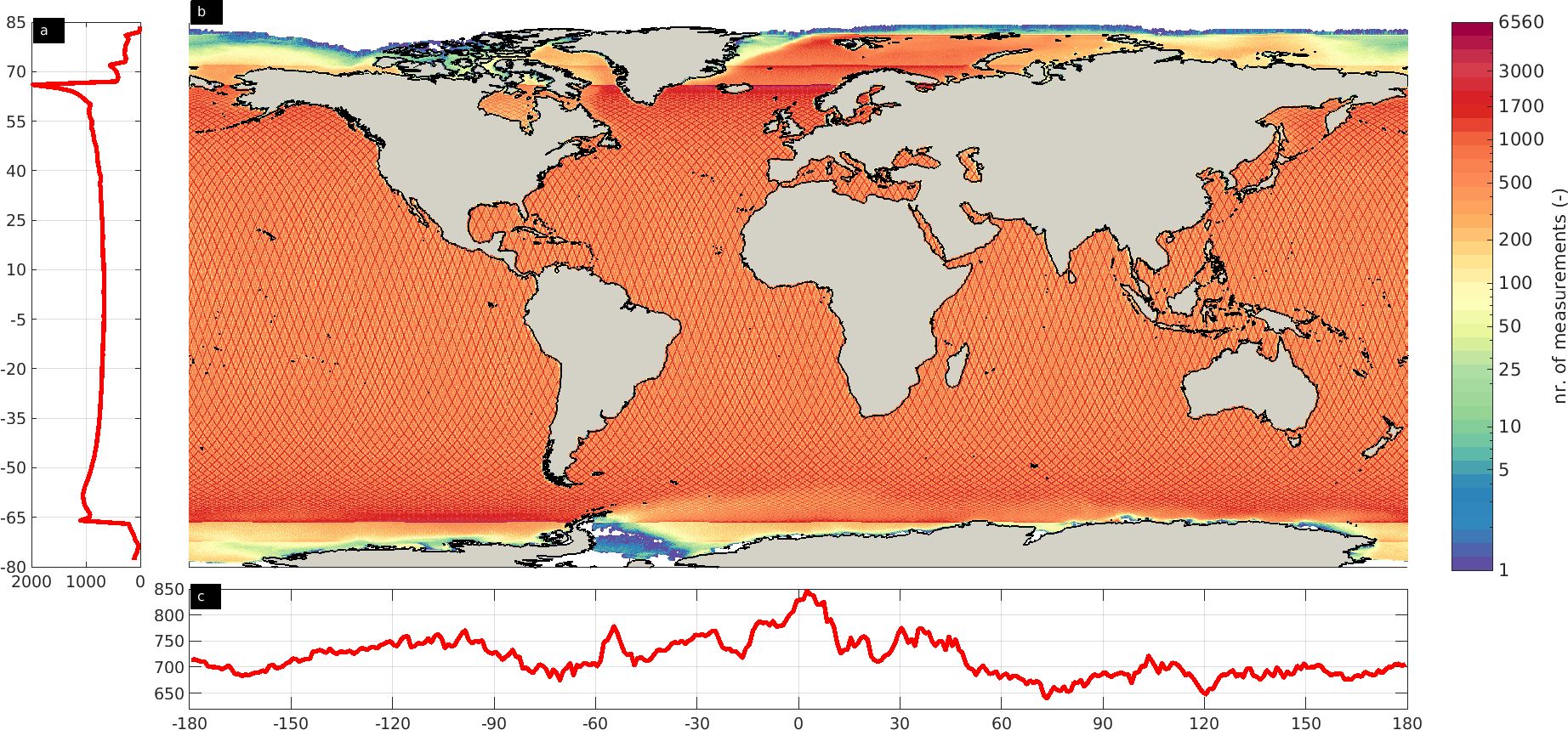
Figure 1. Zonal average (A), meridional average (C) and total number of measurements along the global ocean (B) during the period of study. The zonal and meridional values are averaged over one degree. Areas with zero measurements are indicated in white.

Figure 1 depicts the spatial distribution of the measurements in our study period, 31/12/1992-15/10/2019. As expected, the largest amount of data has been collected at high latitudes (around -/+66°), particularly in the North Atlantic Ocean, the Norwegian Sea and the Davis Strait at the Arctic Ocean, with a ~1980 zonal average number of measurements. In the southern hemisphere, the maximum zonal average is ~1100 measurements, and it is observed in the range [-66°, -58°]. In the subtropics, the zonal average is ~700 measurements. North of 82°N, the amount of measurements is less than 21. Similarly, a clear zonation is observed in the southern hemisphere from 67°S, with less than 210 measurements. This variation suggests either a limited number of missions operating over these areas or possibly the limited validity of the measurements due to the presence of ice. The meridional distribution revealed a peak at [0.5°, 4.5°] with ~830 measurements and a minimum of ~640 measurements observed at 73°E and 120°E.

The spatial distribution between consecutive measurements is presented in Figure 2. The areas with the most frequent measurements are the Norwegian, Irminger and Labrador Seas and the SE South Pacific Ocean, where valid measurements exist from sub-daily to less than 3 days (Figure 2B). An exception are the Norwegian and Laptev Seas and the Arctic Ocean north of ~73°N, where the recurrence period is higher than 50 days, with an average zonal recurrence period from ~2.5 to ~200 days (Figure 2A). For the Antarctic Ocean (south of 66°S), the average zonal recurrence period ranges from 13 to 89 days (Figure 2C). At the north and south temperate zones, the minimum (maximum) mean zonal recurrence period varies from ~2hrs (~9.8 days) to ~1hr (~13.2 days) respectively. Indicatively, the average zonal recurrence period around 7°S is ~1.7 days, potentially reflecting the scarcity of measurements in areas with high density of islands, such as the Banda Sea. Areas with the lowest mean meridional recurrence period are observed at around 104°W (~84 days), 98°W (~81 days) and 60°W (~77 days), while areas with the highest recurrence period are at 54°W (~22.5 days) and 3.5°E (~22 days) (Figure 2C).

Figure 2

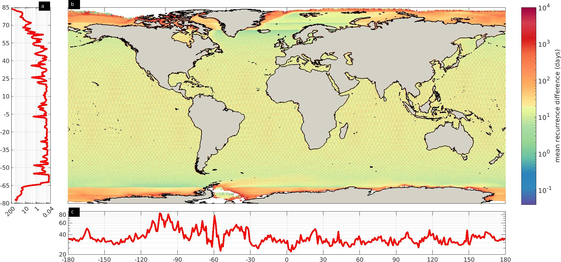
Figure 2. Same as Figure 1 but for the average recurrent days. Areas with no measurements are indicated in white. The zonal, meridional and average recurrence days are plotted in logarithmic scale.

Furthermore, the temporal completeness from 01/01/1993 to 15/10/2019 of the new altimetry dataset has been assessed into four classes, namely <6hrs, (6hrs, 1 day], (1 day, 2 days], (2 days, 3 days] (Figure 3). Measurements in the <6hrs class are especially helpful in identifying episodic WL variations, such as storm events. Low completeness (1-5%) is observed for more than 47% of the global locations, and 5-10% (on average 1/13 measurements) for ~1.8%, ~26%, ~36% and ~33% of the areas for the first, second, third and fourth class respectively. The regions with more frequent measurements ranging from 10% to 50% represent less than 7.9% of the global oceanic coverage, with the <6hr-class exhibiting significantly lower abundance.

Figure 3

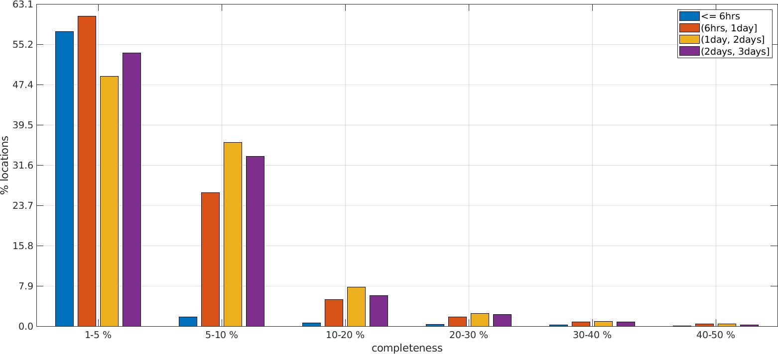
Figure 3. Temporal completeness of the altimeter measurements for the period of study. Note the open left side intervals for the last three classes.

2.2 Tide gauge measurements

Hourly WL measurements were obtained from 5119 TG stations from the GESLA-3 database (Haigh et al., 2022), see Figure 4 for the number of measurements from each TG during the validation period 31/12/1992-15/10/2019. First, for each year and each TG station we removed the tidal level from the yearly WL measurements with the uTide software (Codiga, 2011), and obtained the residual WL. Then, we also removed the outliers in the residual WL measurements that exceeded three times the standard deviation of the corresponding time-series (Sánchez-Román et al., 2020). We utilize the residual WL measurements from the TG stations for the skill assessments that will follow.

Figure 4

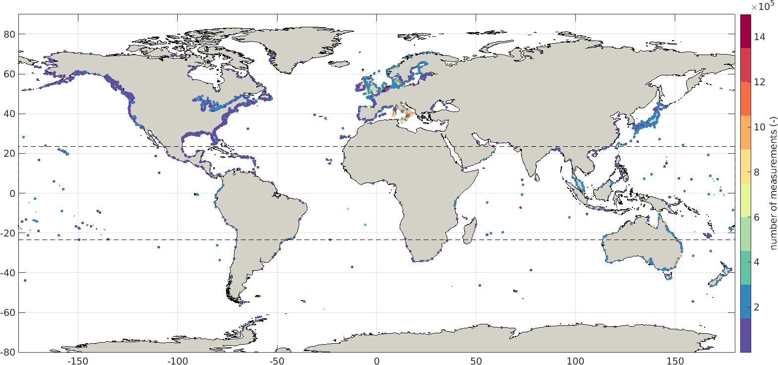
Figure 4. Spatial distribution of the GESLA-3 tide gauge records and the corresponding amount of hourly measurements during the reference period 31/12/1992-15/10/2019. The black dashed lines indicate the two tropics.

2.3 Numerical hydrodynamic data

Both regional (for instance Fernández-Montblanc et al., 2020) and global scale studies (Mentaschi et al., 2023) have utilized the altimetry WL measurements in order to assess the skill of hydrodynamic numerical models, especially in areas where TG data is not available. In this study, we use the 6-hourly SSL from the unstructured hydrodynamic numerical model D-FLOW forced by the European Centre for Medium-Range Weather Forecast (ECMWF) ERA-Interim reanalysis product (Dee et al., 2011). This is the model of Vousdoukas et al. (2018) for the period 31/12/1979-31/12/2014 with predictions at 10780 locations along and offshore from the global coastline. Our aim was to assess the performance of the D-FLOW predictions (Kernkamp et al., 2011; Muis et al., 2016) compared with the altimeter measurements from the current study. Vousdoukas et al. (2018) and references therein describe the characteristics and setup of D-FLOW, as used in the current study.

2.4 Development of the statistical WL models

Following Camus et al. (2014) and Cid et al. (2017), we derive the continuous in time daily maximum WL, by developing a statistical relationship with the local atmospheric conditions as predictors and the altimeter derived WL as the predictand. First, for each altimeter grid point, the 1°x1° (4x4 grid points) daily maximum 10m wind components, the daily minimum mean sea level pressure and daily minimum mean sea level pressure gradients (the latter computed with the surrounding 6x6 grid points) from the ECMWF ERA5 reanalysis product (Hersbach et al., 2020) are extracted and collocated in time with the daily maximum SLAwithDAC WL (see also Cid et al. (2018) regarding the selection of the time lag and timing of the atmospheric conditions and the exclusion of the land nodes). These time-series are standardized to avoid large variance differences in the Principal Components Analysis (PCA) which will follow next.

In particular, PCA is used to convert a dataset with highly correlated variables into linearly uncorrelated factors called principal components. This transformation is achieved by identifying the eigenvectors and eigenvalues of the covariance matrix of the original dataset, where the eigenvectors represent the directions of maximum variance, and the eigenvalues indicate the magnitude of this variance. Mathematically, the conversion of the original data matrix X into the principal component scores Z can be expressed as:

$\begin{array}{ll}Z=X*W& (5)\end{array}$

where W is the matrix of eigenvectors.

While a linear PCA assumes a linear relationship among the variables, which may not always hold true, this assumption can be considered reasonable given the large dataset and extensive geographical coverage.

Then, the principal components (PC) that explain 95% of the variance in local atmospheric conditions are selected and a multivariate linear regression model (hereafter referred to as PCVAR) is fitted with the daily maximum SLAwithDAC water levels. Aiming to further reduce the PC dimensionality, a second multivariate linear regression model (hereafter, PCSTEP) is developed applying a stepwise regression fit of the atmospheric conditions PC with the daily maximum SLAwithDAC WL, until no significant improvement of the model is observed at the conventional 5% level of significance. The WL from the PCVAR and PCSTEP models is estimated with:

$\begin{array}{ll}WL=a_1+b_1*P{C}_1+b_2*P{C}_2+\dots +b_n*P{C}_n& (6)\end{array}$

where WL is the daily maximum WL, a1, b1,…, bn are the coefficients obtained either from the PCVAR or the PCSTEP models, and PCx are the principal components of the standardized atmospheric conditions.

The internal consistency of the PC is assessed using the Cronbach-alpha coefficient (Cronbach, 1951), considered adequate for values higher than 0.6 (Hair et al., 2010). Finally, the continuous daily maximum WL time-series for the period 31/12/1992-31/10/2019 are computed from the daily (maximum) 10m U, V wind components and (minimum) mean sea level pressure and pressure gradients from the ECMWF ERA5 reanalysis atmospheric conditions and their PC coefficients.

In order to evaluate the robustness of utilizing the satellite derived WL data, a third multivariate linear regression model is developed (hereafter, PCWN) by fitting the PC of the atmospheric conditions to an additive white Gaussian noise signal (Graffigna et al., 2019). The null hypothesis that the distribution mean of the PC regression analysis of the satellite data equals the distribution mean of the PCA with white noise, this is tested with the one-way analysis of variance (ANOVA) at the 5% significance level.

2.5 Performance metrics

To ensure data reliability and address uncertainties stemming from the sparse temporal alignment between tide gage record, numerical model data and altimetry measurements, we have followed the central limit theorem, which requires that the sampling distribution of the sample mean converges to a normal distribution for samples with more than 30 observations (Ross, 2021). Consequently, TG stations that contain less than 30 measurements were excluded from this analysis. This filtering ensures our adherence to statistical best practices and upholds the integrity of our data. Nevertheless, we also recognize the significance of thorough validation in our study. The performance of the altimeter derived WL with the TG records and the D-FLOW numerical hydrodynamic data, as well as the statistical reconstructed daily maximum WL with the TG records is assessed with three performance metrics, which assume a normally distributed sample size, consistent with standard validation practices. These three are the percentage root mean squared error (%RMSE), the bias, and the modified Mielke lamda-index (λ) (Duveiller et al., 2016) which combines the correlation coefficient and the RMSE, and they are defined by the following equations:

$\begin{array}{ll}\%RMSE=\frac{100*\sqrt{\frac{1}{n}{{\displaystyle \sum }}_{i=1}^n{(w{l}_1-w{l}_2)}^2}}{max(w{l}_1)}& (7)\end{array}$

$\begin{array}{ll}BIAS=\frac{1}{n}{\displaystyle \sum }_{i=1}^n(w{l}_1-w{l}_2)& (8)\end{array}$

$\begin{array}{ll}\lambda =1-\frac{\frac{1}{n}{{\displaystyle \sum }}_{i=1}^n{(w{l}_1-w{l}_2)}^2}{{\sigma }_{wl1}+{\sigma }_{wl2}+{(\overline{w{l}_1}+w{l}_2)}^2+\kappa }& (9)\end{array}$

where,

$$\kappa =0,\rho >0$$

$$\kappa =2\ast \left|{\displaystyle {\displaystyle \sum }_{i=1}^n}(w{l}_1-\overline{w{l}_1})\ast (w{l}_2-\overline{w{l}_2})\right|,\rho \ne 0$$

with

ρ being the Pearson correlation coefficient

$\begin{array}{ll}\rho =\frac{1}{n-1}{\displaystyle \sum }_{i=1}^n\frac{(w{l}_1-\overline{w{l}_1})}{{\sigma }_{wl1}}\times \frac{(w{l}_2-\overline{w{l}_2})}{{\sigma }_{wl2}}& (10)\end{array}$

wl1 are the time-series from the TG, and wl2 are the time-series of the particular satellite WL component (namely SLAnoDac, SLAwithDAC or DAC) compared with the TG data. For the validation of the D-FLOW data vs the satellite data, wl1 are the SSL time-series from the D-FLOW model and wl2 again are the satellite derived WL components (SLAnoDac, SLAwithDAC and DAC).

3 Results

3.1 Validation and intercomparison of the altimeter WL data

Here, we compare the SLAnoDac, SLAwithDAC and DAC with the GESLA-3 TG measurements and with the D-FLOW numerical data, to evaluate their performance, aiming to examine the contribution of each of the components to the water level. Then, we present the validation of the continuous-in-time statistical reconstructed daily maximum WL during the altimeter period 31/12/1992-31/10/2019, with the tidal gauge timeseries.

3.1.1 Altimeter WL data compared to tide gauge measurements

We now compare the altimeter WL components with all 4593 GESLA-3 TG stations measurements, in the period 31/12/1992 23:00:00 - 31/10/2019 23:00:00 where both time-series exist. Due to the temporal sparsity between the collocated TG and altimetry data and following the central limit theorem we exclude TG stations that contain less than 30 measurements. We evaluate individual TG measurements within 1hr from each altimeter measurement, assuming that the hourly WL variations are representative. Moreover, we consider only TG stations that are located less than 25 km from the closest altimeter grid node. We are thus left with 1686 TG records worldwide.

In Figure 5 we present two performance metrics the bias and the λ-index and compare the TG measurements and the three altimeter components (see also Supplementary Figure S3 for the %RMSE performance metric). Regarding the SLAnoDAC component, ~76% of the areas exhibit a positive bias up to 0.08m, while at 55 TG stations the bias is negative, e.g. in the Black Sea (0.26m), the English Bight (0.08m) and the tropical zone of the W Pacific Ocean (0.06m), see Figure 5A. About 68% of the areas appear with less than 46% %RMSE (Supplementary Figure S3A), while the λ-index for 66% of the areas is less than 0.6, and for ~5% of the areas, the λ-index ranges from 0.6 to 0.8 (Figure 5B). At ~67% of the areas the SLAwithDAC component exhibits a positive bias <0.1m (Figure 5C), ~60% of the areas are characterized by a good to perfect skill (λ-index >0.6) (Figure 5D) and ~72% of the areas have %RMSE less than 40% (Supplementary Figure S3C).

Figure 5

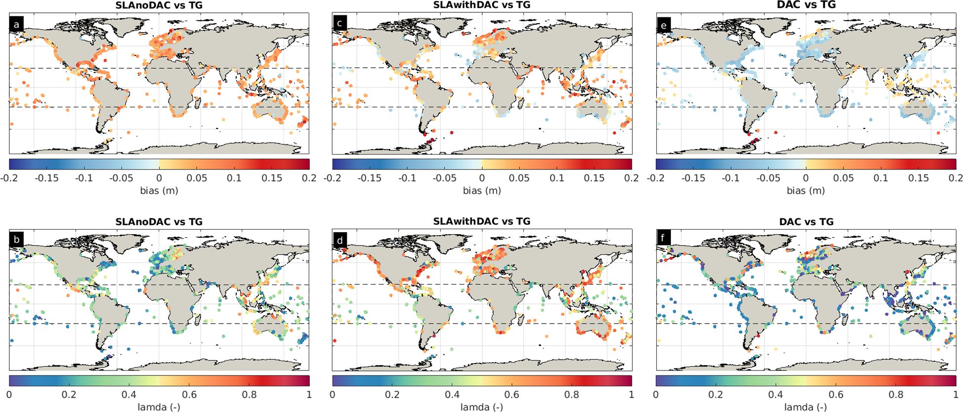
Figure 5. Validation of the SLAnoDAC (A, B), SLAwithDAC (C, D) and DAC (E, F) altimeter water level components with the tide gauges timeseries, in terms of the bias (top row) and the λ-index (bottom row). The black dashed lines indicate the two tropics.

Worse skill is observed at the tropical zone (the area defined between the latitudes -/+23.4364°) where the average λ-index is 0.48 and the average %RMSE is 48.7%. The DAC component exhibits a negative bias > -0.1m at ~90% of the areas, while ~50% of the areas are characterized by less than 0.05m bias. Areas with positive bias are the tropical zone of the Indian Ocean and the W Pacific Ocean, the Bering Sea and the Norwegian Sea (Figure 5E). The DAC component exhibits the best performance mainly at the North Sea, with good skill and average λ-index = 0.75 (Figure 5F). As is the case for many hydrodynamic models, at the tropical zone the skill is not adequate, with an average λ-index = 0.26, and average %RMSE ~41% (Supplementary Figure S3E).

3.1.2 Altimeter WL measurements compared to hydrodynamic numerical model data

As we did with the previous comparisons, for each D-FLOW model output location within a distance less or equal to 25 km from the altimeter grid node, we selected only the SSL elevations that are within 1hr from the altimeter measurements. We found that 2607 time-series collocated with the TG stations and we used them for intercomparing the D-FLOW data with the three altimeter components.

When the altimeter components and the D-FLOW data are compared, it is clear that the contribution of the DAC component is critical, as by itself it is a hydrodynamic model output. The SLAnoDAC component exhibits a positive bias of ~0.08m (e.g. at the N Atlantic Ocean and the S Indian Ocean), except for the E Bering and the Gulf of Alaska, the Baltic Sea and the Tropical zone of the E Indian Ocean and the W Pacific Ocean where the average bias is lower (-0.03m) (Figure 6A). The majority of the areas (~97%) exhibit poor performance with the λ-index <0.4 (Figure 6B) and the average %RMSE=115.5% (Supplementary Figure S3B). When the DAC correction is not applied to the SLA measurements, the average bias is reduced by about 57% (0.04m compared to 0.07m with the DAC correction) (Figure 6C), the average λ-index is 0.5 (Figure 6D) and the average %RMSE is ~86.1% (Supplementary Figure S3D). At the tropical zone, the agreement between the SLAwithDAC and SLAnoDAC is slightly improved. As expected, the inter-model comparison between the DAC and the D-FLOW numerical data exhibits better agreement compared to the SLAwithDAC data, with the average bias equal to 0.006m (Figure 6E). We observe moderate performance (average λ-index 0.54), even at some parts of the Tropical zone, such as the Gulf of Mexico, the Caribbean Sea, the E Atlantic Ocean and the central Indian Ocean (Figure 6F).

Figure 6

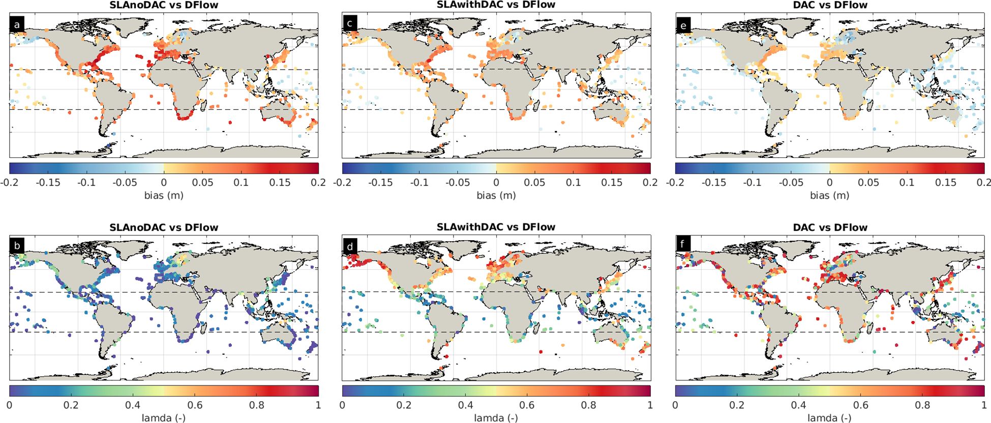
Figure 6. Same as Figure 5, but here we compare the water level from the D-Flow model and the SLAnoDAC (A, B), SLAwithDAC (C, D) and DAC (E, F) altimeter water level components.

3.1.3 Continuous temporal statistical reconstructed altimeter WL compared with tide gauge records

Here, we address the question whether we can use existing sparse measurements for long term hindcasts. The results in the previous two subsections suggest that the discontinuous temporal SLAwithDAC WL component performs better than the discontinuous SLAnoDAC or DAC components, when compared to TG measurements. Additionally, the λ-index of the SLAwithDAC component is similar to the one of the DAC component, when compared to the D-FLOW numerical data. In this subsection, the daily maximum SLAwithDAC WL during the period 31/12/1992-31/10/2019 is our predictand of the PCVAR and PCSTEP multivariate linear regression models with the time collocated atmospheric conditions from the ECMWF ERA5 reanalysis dataset, in order to derive the principal components of the atmospheric conditions for every node of our 0.25°x0.25° global ocean grid. The aim is to reduce the temporal scarcity of the altimeter measurements and derive a continuous daily maximum SLAwithDAC WL for the 31/12/1992-31/10/2019 period. We will then check the validity by comparing the derived daily maximum WL from PCVAR, PCSTEP and PCWN with the daily maximum residual water levels from the GESLA-3 TG records.

For each TG record with more than 30 daily collocated measurements, we select the daily maximum WL data from the altimeter grid node less than 25 km apart. This filtering results in 2164 TG records, whose spatial distribution and the corresponding performance metrics are presented in Figure 7. For the time-series examined, the Cronbach-alpha coefficient is higher than 0.65 indicating the high internal consistency of the PC (see Supplementary Figure S4B). Additionally, the one-way ANOVA test indicates that when the SLAwithDAC WL component is utilized, 2091 out of the 2164 examined WL timeseries are significantly different from the corresponding ones derived from the PCWN regression model (see Supplementary Figure S4C). This is a first evidence that when the altimeter measurements are utilized the constructed timeseries present significant variability with respect to the corresponding ones from the PCWN model.

Figure 7

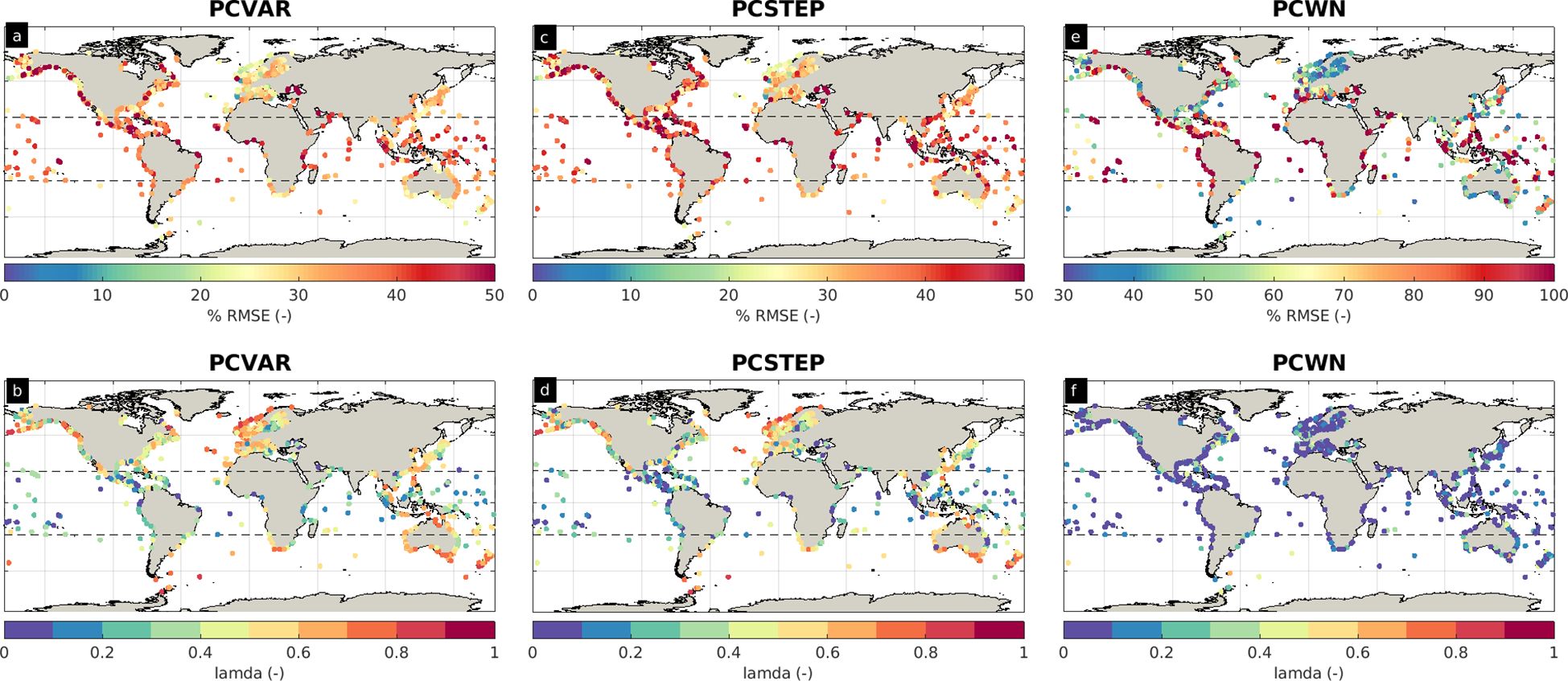
Figure 7. %RMSE and λ-index of the water level estimated by the PCVAR (A, B), PCSTEP (C, D) and PCWN (E, F) models vs the tide gauge records. Note the different scale of the %RMSE metric of the PCWN model, compared to the other two models. The black dashed lines indicate the two tropics.

In Figure 7, we present the spatial distribution of the %RMSE and the λ-index performance metrics along the global coastline between the reconstructed WL estimated by the three models and the TG records. We note that the average bias between the TG WL time-series and each of the three models is less than 10^-5m (not shown). The PCVAR and the PCSTEP models indicate similar %RMSE with a global average equal to ~34.01% (Figure 7A) and ~38.5% (Figure 7C) respectively, while the global average %RMSE of the time-series from the PCWN model is ~73.9% (Figure 7E). Excluding the tropics, the global average %RMSE for PCVAR is ~32.7% and for PCSTEP is ~37.1%. Regarding PCVAR, around ~42% of the areas are described by %RMSE less than 30.0% (Figure 7A), while ~68% of the areas demonstrate a reasonable to excellent skill with λ-index ranging from 0.4 to 0.87, see Figure 7B. About 30% of the time-series from PCSTEP exhibit %RMSE less than 30% and ~51% of the areas are characterized by reasonable to excellent skill (Figure 7D). Furthermore, PCVAR estimates fewer time-series where the skill is poor (λ-index<0.3) compared to PCSTEP. The fact that ~90% of the time-series from the PCWN model are described with λ-index less than 0.3, is indicative that the PC of the atmospheric conditions alone do not suffice to estimate the WL (Figure 8). Only six time-series from PCWN that are not significantly different from PCVAR model exhibit skill from 0.4 to 0.59.

Figure 8

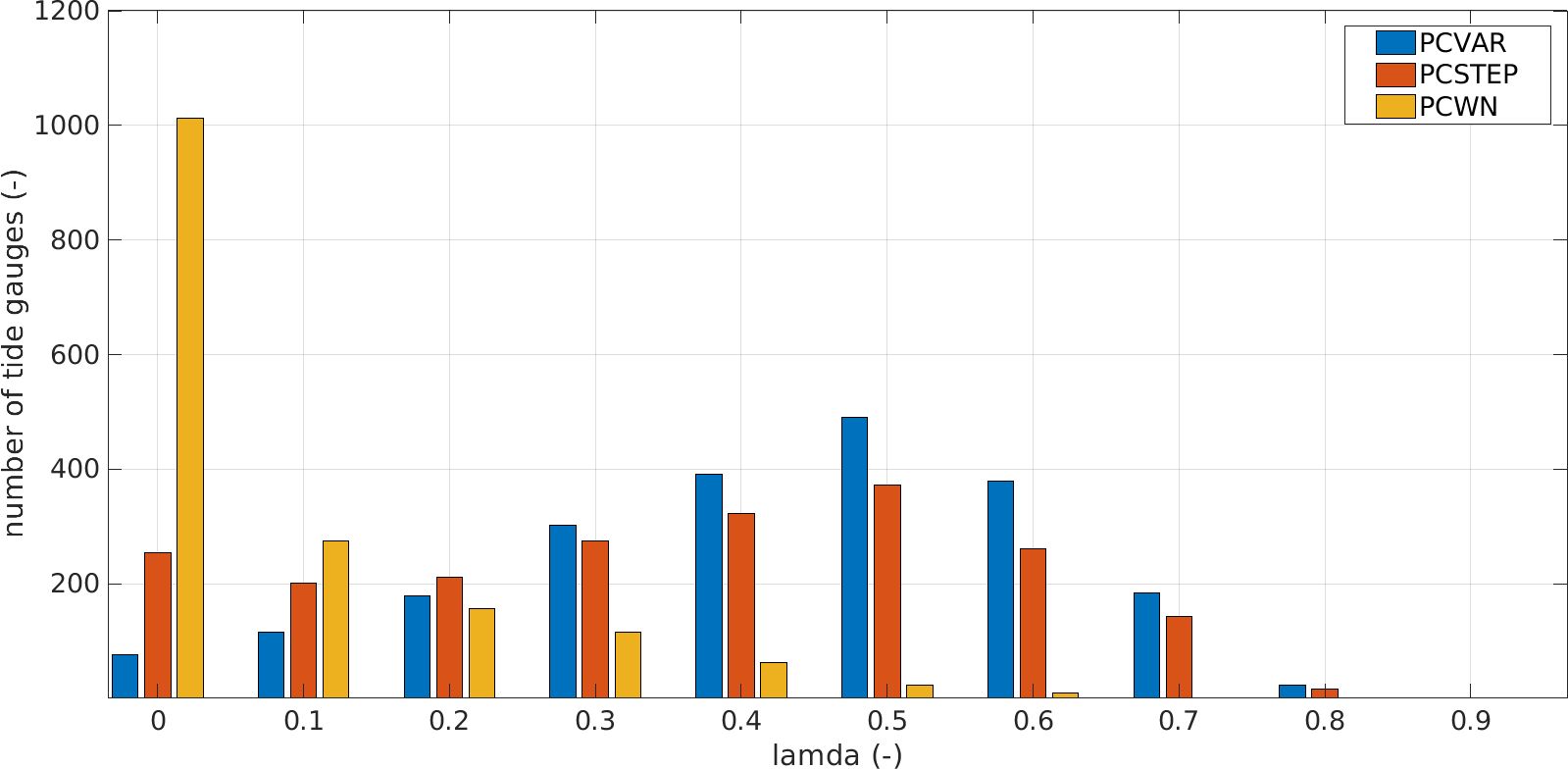
Figure 8. Distribution of the λ-index from PCVAR (blue bars), PCSTEP (red bars) and PCWN (yellow bars) multivariate linear regression models validated with the tide gauge measurements for the period 1992-2019.

Table 1 presents the performance metrics between the TG timeseries and the PCVAR and PCSTEP. For both models, regions characterized by reasonable to good skill are:

● the Irish Sea (λ-index up to 0.78 and average %RMSE ~26.8, λ-index up to 0.78 and average %RMSE ~27.6 for PCVAR and PCSTEP respectively),

● the North Sea except for the E coast of the UK (λ-index up to 0.87 and average %RMSE ~24.9, λ-index up to 0.81 and average %RMSE ~26.7 for PCVAR and PCSTEP respectively),

● the Gulf of Lion and the W Ligurian Sea (λ-index from 0.5 to 0.7 and average %RMSE ~27.0, λ-index from 0.1-0.68 and average %RMSE ~30.7 for PCVAR and PCSTEP respectively),

● the W Labrador Sea (λ-index up to 0.82 and average %RMSE ~36.1%, λ-index up to 0.73 and average %RMSE ~38.8 for the PCVAR and PCSTEP respectively),

● the Gulf of Alaska (λ-index up to 0.87 and average %RMSE 43.9, λ-index up to 0.87 and average %RMSE ~47.1% for the PCVAR and PCSTEP respectively),

● the SE Australian continent and the New Zealand (λ-index ranging from 0.5 to 0.8 and average %RMSE ~25.5%, λ-index from 0.1 to 0.8 and average %RMSE ~27.7 for the PCVAR and PCSTEP respectively),

● and the S Atlantic Ocean below 34°S (λ-index ranging from 0.54 to 0.87 for both of the models and average %RMSE ~27.5 and ~29 for PCVAR and PCSTEP respectively).

Although at the tropics, the overall λ-index is low (less than 0.4 at 64% and 74% of the locations for PCVAR and PCSTEP models respectively) and the average %RMSE of PCVAR is ~32.7 (~37.1 for PCSTEP), at the SW South China Sea, the Java Sea and the Banda Sea the λ-index ranges from 0.5 to 0.7 (0.4 to 0.7 for PCSTEP) and the %RMSE is ~30.8 for PCVAR (~34.5 for PCSTEP). Apart from the tropics, regions that demonstrate not adequate to average skill are:

● the Baltic Sea (45% of the areas with λ-index less than 0.4 for both models and average %RMSE 30.2 and 31.9 for PCVAR and PCSTEP),

● the Black Sea (λ-index < 0.4 and average %RMSE 202.7, λ-index < 0.3 and average %RMSE 284.7 for PCVAR and PCSTEP respectively),

● the Gulf of Mexico except for the eastern part (65% of the areas with λ-index < 0.4 for PCVAR and average %RMSE 33.3, 73% of the areas with λ-index less than 0.4 and average %RMSE ~38.0 for PCVAR and PCSTEP),

● and the subtropical zones of the NW Atlantic Ocean and of the S Pacific Ocean.

Table 1

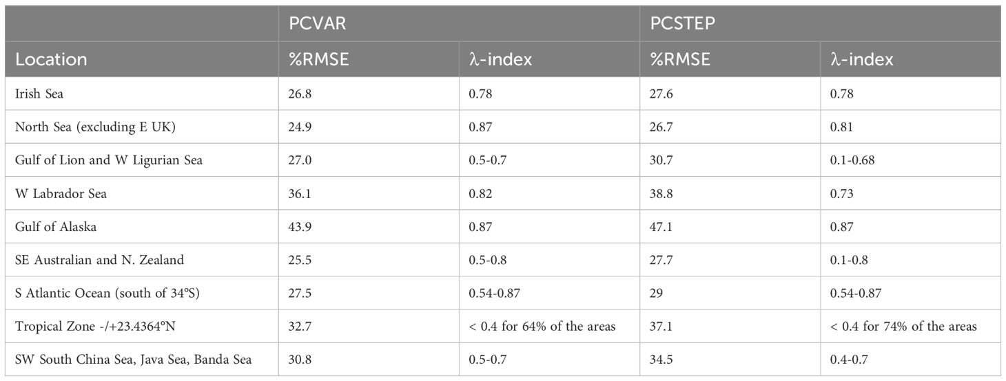
Table 1. Performance statistics between the tide gauge stations and the PCVAR and PCSTEP models.

3.2 Applications

3.2.1 62 years of daily maximum ocean water level hindcast

Here, we use the coefficients from PCVAR with the atmospheric conditions from the ECMWF ERA5 reanalysis dataset, for the period 1/1/1959-31/12/2021, in order to reconstruct the continuous-in-time daily maximum WL, at each 0.25°x0.25° node of our altimeter grid. The maximum daily maximum WL for the 62-year period (Figure 9) reveals qualitatively the main global ocean circulation patterns, such as the western boundary currents (e.g. the Kuroshio current in the NW Pacific Ocean, the Gulf Stream), eastern boundary currents (e.g. the South Equatorial and Benguela current in SW Africa), and equatorial waves (Andres et al., 2008; Dohan, 2017). Additionally, Figure 9 further outlines the distribution of high-frequency small-scale features such as eddies in regions of intense circulation (Chelton et al., 2011; Faghmous et al., 2015). Moreover, areas with increased WL are the N Atlantic Ocean, the N Pacific Ocean and the Bering Sea, the East China Sea, the East Bay of Bengal, the Arafura Sea and the Southern Ocean.

Figure 9

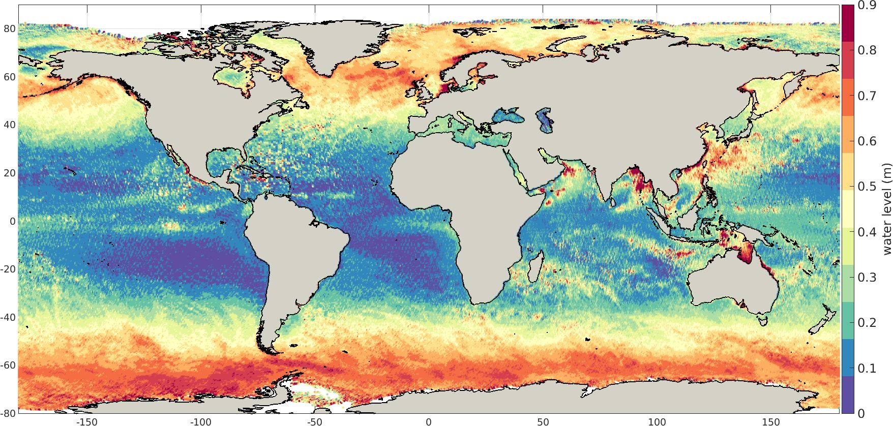
Figure 9. Maximum daily maximum water level (m) for the period 1/1/1959-31/12/2021 estimated by PCVAR model.

Figure 10 presents the statistical reconstructed WL timeseries from the PCVAR model collocated in time with the closest TG WL time-series (panels A-F) and their corresponding skill metrics (panels G-L). The PCVAR model time-series show a better agreement with TG records at high latitudes, e.g. Aalesund, Norway, Base Prat, Chile and Mornington island, Australia with %RMSE equal to 13.64, 15.32, 17.58 and λ-index equal to 0.73, 0.82 and 0.64 respectively. A lower model performance is observed at low latitudes, where only the long WL variations are estimated reasonably well in Pointe Noire, Congo and Chittagong, Bangladesh. It needs to be further examined, whether the lower model performance such as of the last two locations, may be attributed to the low amount of the original sparse altimeter measurements, as described in subsection 2.1 of this study.

Figure 10

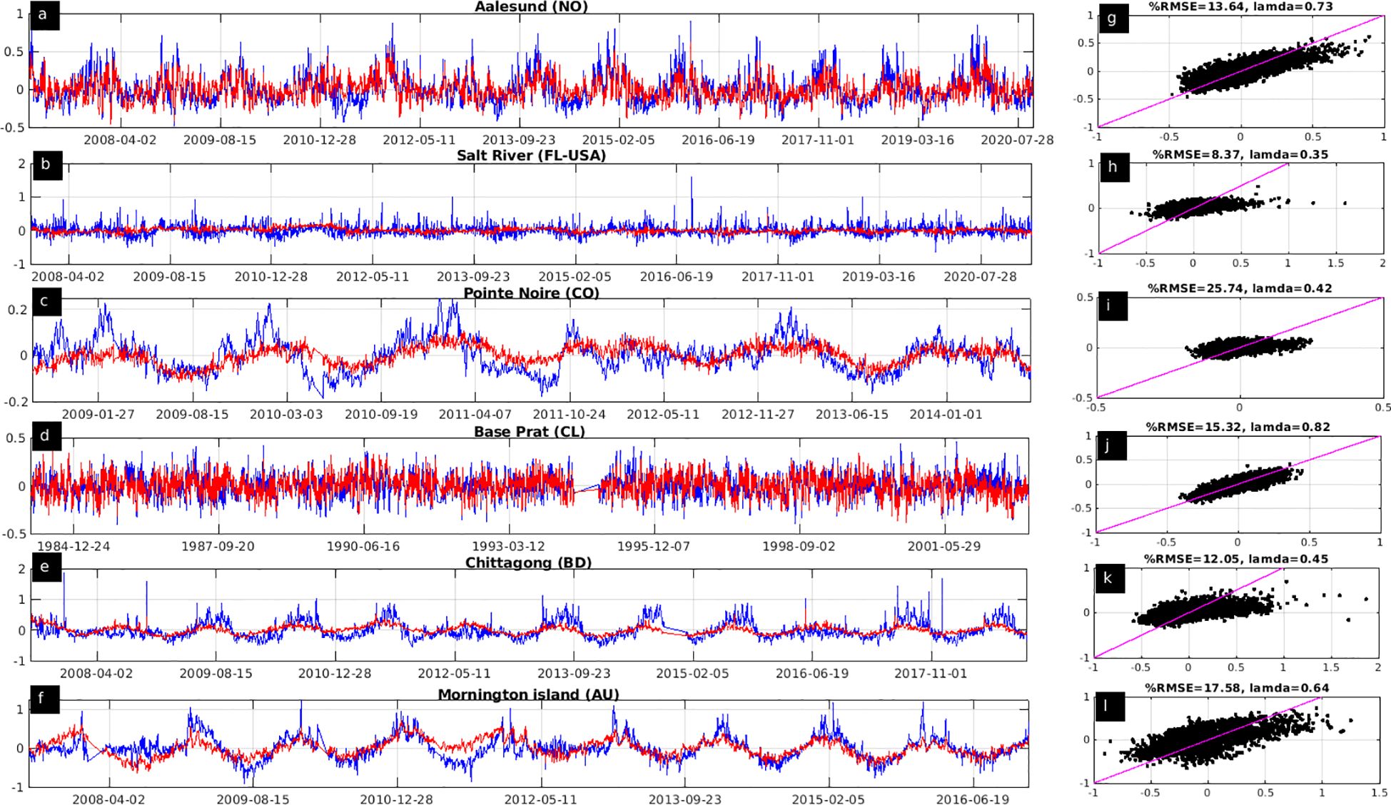
Figure 10. Daily maximum water level (m) from the tide gauge records (blue lines) and from PCVAR model (red lines) (panels A-F) and the corresponding scatter plots vs the perfect-fit line (black dots and magenta lines, at panels G-L) at Aalesund (Norway), Salt River (Florida, USA), Pointe Noire (Congo), Base Prat (Chile), Chittagong (Bangladesh) and Mornington island (Australia) tide gauge stations.

3.2.2 Tropical cyclone induced water level

The year 2018 was one of the most active on record in terms of tropical cyclone (TC) activity, with 23 TCs occurring in September and more than 12 concurrent tropical cyclones in the Atlantic, Pacific and Indian Ocean⁴. Figure 11 shows the 47 TC tracks from the IBTrACS archive (Knapp et al., 2018, 2010) from 1/8/2018 to 15/10/2018. The daily maximum WL from PCVAR for the same period is presented in Figure 12. The tropical cyclone paths are evident at the oceanic surface, particularly over the Central and N Atlantic Ocean, the Gulf of Aden, the Philippine Sea and the East China Sea. This observation highlights how PCVAR can qualitatively estimate global water levels during periods of highly energetic atmospheric conditions.

Figure 11

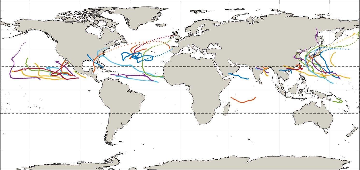
Figure 11. Tropical cyclone paths from the IBTrACS archive during the period 1/8/2018-15/10/2018, with each colour and track representing a different event.

Figure 12

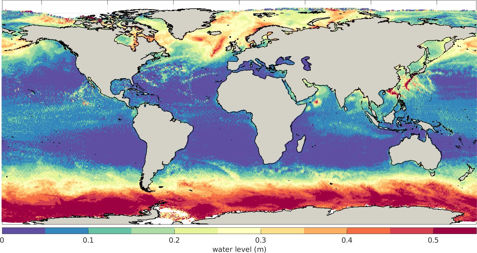
Figure 12. Maximum daily water level as estimated by PCVAR model during the period 1/8/2018-15/10/2018.

The validation results with the six TG water level time-series are presented in Figure 13, (panels A-F), along with the corresponding performance metrics (Figure 13, panels G-L). PCVAR reproduces quite well the WL during the peak of the TC induced WL in Naja (Japan). Good agreement is observed between the TG and the PCVAR time-series at Currimao (Philippines), Ballyglass (Ireland) and Dingle Harbor (Ireland) where although the peak WL is underestimated the TG and model time-series are in phase. At Fort Point, New Hampshire and North Spit, California, TG the skill is reasonable and the %RMSE is ~22.7 and ~29.4 respectively, much as the WL range during this period is low.

Figure 13

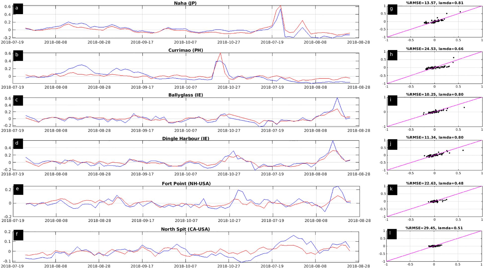
Figure 13. Daily maximum water level (m) during the period 1/8/2018-15/10/2018 from the tide gauges (blue lines) and from the PCVAR model (red lines) (panels A-F) and the corresponding scatter plots vs the perfect-fit line (black dots and magenta lines, panels G-L) at Naha (Japan), Currimao (Philippines), Ballyglass (Ireland), Dingle Harbour (Ireland), Fort Point (New Hampshire, USA) and North Spit (California, USA) tide gauge stations.

As an example, for this 45-day period of intense tropical cyclone activity, we compare the open ocean water levels from PCVAR with the WL resulting from the linear addition of SLA L4 measurements (https://doi.org/10.48670/moi-00144) with the DAC component (10.24400/527896/a01-2022.001). In contrast to the L3 dataset we utilize, the DAC component is not available in the SLA L4 dataset. After downloading the 6-hourly DAC component, we identified its closest grid nodes in the SLA L4 grid, and then computed the daily maximum WL, including the contribution of the L4 and DAC. We refer to this as L4+DAC.

The comparison between the daily maximum WL obtained by the PCVAR model and the L4+DAC is presented in Supplementary Figure S5. The spatial distribution of the %RMSE and the λ-index indicates better agreement at high latitudes with the overall %RMSE > 20% for ~71% and above 0.7 for ~42% of the ocean surface, respectively. The agreement between the two datasets is higher along the TC tracks (as also shown in Figure 12) at the N Atlantic Ocean and the NE Pacific Ocean, with lower %RMSE and higher λ-index. Except for the tropics, areas characterized by higher %RMSE and lower λ-index are those with high SLA variability (Ballarotta et al., 2023), such as offshore SE South America, the NE North America, the NW Pacific Ocean and the E Siberian Sea. Similarly, at these areas the coupled storm surge and wave numerical model by Mentaschi et al. (2023) exhibited larger model deviations when validated with altimeter data. It is worth noting that the bias between the two datasets is low and its range is -/+0.1cm for ~96% of the areas.

Indicatively, the comparison of the time-series at six locations between the L4+DAC and PCVAR daily maximum WL along with the available L3 WL measurements is presented in Supplementary Figure S6. Despite the overall scarcity of the L3 measurements (red stars) which inform PCVAR (blue line), good agreement is observed with the L4+DAC (black line), with λ-index > 0.6 and %RMSE < 18.3 (panels A-D and G-J, in Supplementary Figure S6). Moreover, while none of the peak WL events were recorded by the L3 dataset, PCVAR accurately estimated these high intensity events, in good agreement with the L4+DAC data. The peak events (as in Supplementary Figure S6B, on 2018-10-22) recorded at the L3 dataset but neither by the L4+DAC nor from the PCVAR model, they need to be further examined to understand whether they are not triggered by intense atmospheric conditions. However, these events do not appear to mislead either the L4+DAC or PCVAR. The cases presented in panels E and F of Supplementary Figure S6, demonstrated the limited agreement between the L4+DAC dataset and the PCVAR, although the latter seems to be aligned with the L3 records.

3.2.3 15-day medium-term ensemble water level forecast

Working as in subsections 3.2.1. and 3.2.2, we apply PCVAR using the 51 ensemble member ECMWF (ECMWF ENS)⁵ forecast atmospheric conditions, aiming to derive the corresponding WL forecasts at the global ocean, specifically for the 15-day period, 25/09/2018-10/10/2018. For this period, the 10m wind components and the mean sea-level pressure from the medium range 51 ensemble members were first interpolated down to the 0.25°x0.25° grid. Then, the daily maximum wind components, the minimum pressure and the pressure gradients were calculated. Due to the short forecast period of 15 days, in this demonstration we derived a second set of PC coefficients with PCVAR for each grid node and for the entire altimeter period 31/12/1992-31/10/2019, following subsection 3.1.3. However, in this case we used the non-standardized ERA5 reanalysis atmospheric conditions, instead of the standardized ones. The validation of the PCVAR WL with the GESLA-3 TG records is similar as in subsection 3.1.3 and is not shown.

Figure 14A shows the global ocean 15-day probability that the daily maximum WL forecasts will exceed the 99.5th percentile of the ECMWF ERA5-driven daily maximum WL hindcast (subsection (3.2.1)). We estimated probabilities using the 51 ensemble member ECMWF ENS. PCVAR estimates with high probability of exceedance the landfall of tropical cyclone Kong-rey offshore Japan and Taiwan, Hurricane Leslie at N Atlantic Ocean and Hurricane Rosa offshore W Mexico, as well as the induced water level (Figure 14C). The ensemble median daily maximum WL from PCVAR (green line in Figure 14C) is in good agreement with the GESLA-3 Hirarako TG record (black line in Figure 14C) for the first seven days of the forecast (25/09/2018-01/10/2018). PCVAR accurately estimates the ensemble-median WL peak on 28/09/2018, despite being forced with the ECMWF ENS atmospheric forecast, issued four days before the actual cyclone-induced WL peak recorded at the Hirarako TG station. According to the GESLA-3 TG stations in Kushiro and Esashiko, the WL peak was recorded on 01/10/2018 (black lines in Figure 14D, E, respectively), seven days after initializing the PCVAR forecast (blue lines in Figure 14D, E, respectively), which accurately estimates the arrival time of the WL peak. The ensemble-median forecast WL peak from PCVAR appears lower than in the TG records, an indicator of the degrading forecast skill after seven days of both the atmospheric and the PCVAR models.

Figure 14

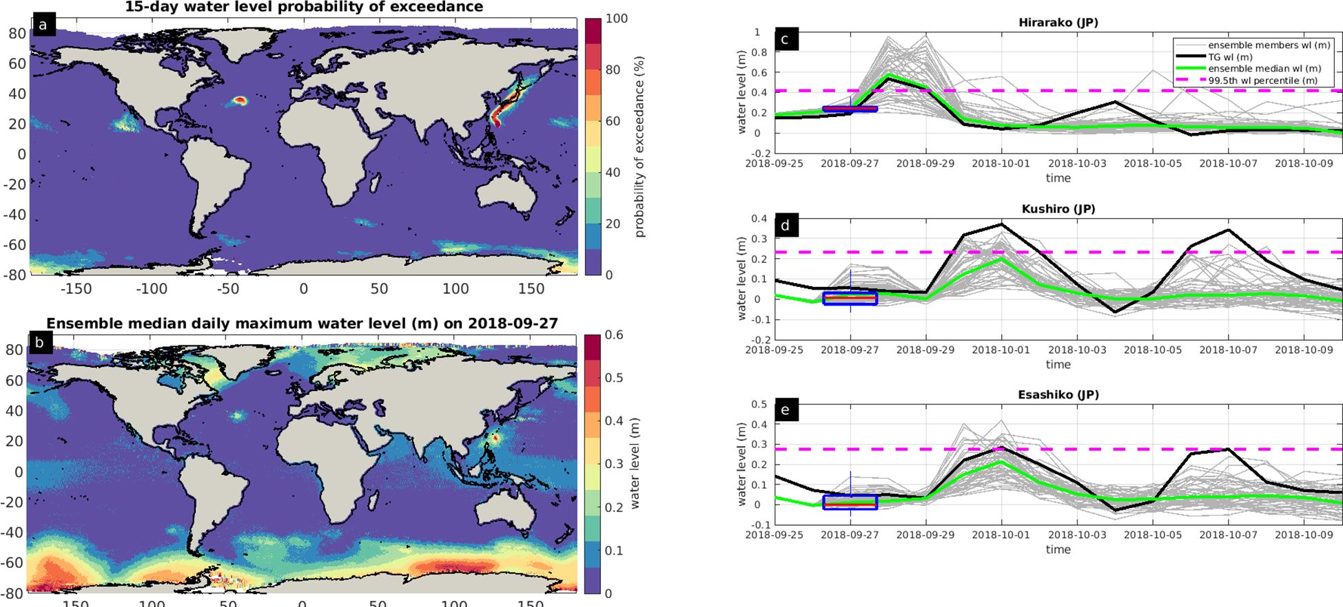
Figure 14. Daily maximum water level (m) forecast exceedance probability of the PCVAR ECMWF ERA-5 hindcast daily maximum water level during the period 25/09/2018-10/10/2018 (A). Ensemble median daily maximum water level (m) on 27/09/2018 (B). Daily maximum water level from the GESLA-3 tide gauge records (black solid line) and the corresponding 51 ensemble members daily maximum water level (grey solid lines) and ensemble median daily maximum water level (green solid line) estimated from the PCVAR model at Hirarako (C), Kushiro (D) and Esashiko (E) tide gauge stations in Japan. The 99.5th percentile from the PCVAR ERA-5 hindcast water level is indicated by the magenta dashed line. The box plots display the 25th and 75th percentile of the 51 ensemble members daily maximum water level and the red line the ensemble median daily maximum water level.

4 Discussion

We assessed and demonstrated the feasibility of using detided sparse satellite water level measurements to estimate the water level at the open ocean during highly energetic atmospheric events. Aiming to complement the effort of obtaining high frequency water level estimates, first, we evaluated the temporal and spatial distribution of all the available along-track DT DUACS L3 altimeter water level measurements.

A preliminary validation of the altimetry measurements was performed with the detided GESLA-3 tide gauge records. In order to overcome both the temporal and the spatial scarcity of the tide gauge data, but also to identify the contribution of each one of the altimeter components, we assessed the validity of the altimetry measurements also with 6-hour water level from the validated hydrodynamic unstructured numerical model D-FLOW. Both validation assessments revealed regions with variable performance when different altimeter components were considered. Overall, the altimeter sea-level anomalies after being corrected both with the long-wavelength error component and the tidal level (but without applying the dynamic atmospheric correction), they exhibit better agreement with the tide gauge measurements and with the D-FLOW numerical data. In fact, this indicates that the water level is more accurately represented when the altimeter sea level anomaly measurements are not corrected by a hydrodynamic numerical model with similar spatial resolution. At the tropical zone, the lower agreement between all the examined water level components highlights where the hydrodynamic models need improvements.

Our study underscores how the daily maximum water level due to episodic high energetic atmospheric conditions and persistent sea level currents can be estimated from altimetry data, in conjunction with the local atmospheric conditions. We developed two multivariate linear regression models and checked their skill in reproducing the continuous daily maximum water levels spanning 27 years in comparison with the GESLA-3 tide gauge records. Indicatively, ~11% more tide gauge records were used for the validation of the statistical derived water level, compared to the original temporally sparse altimeter measurements, a potential indication that the temporal scarcity of altimeter measurements may be reduced even further by deploying simple statistical models.

Despite the simplicity of the two statistical models and the inherent temporal scarcity of the altimeter measurements, we demonstrated that the inferred water level from these two models exhibited a reasonable to excellent skill (λ-index 0.4 to 0.8) at ~68% and ~51% of the tide gauge records respectively. Moreover, we showed that atmospheric conditions alone do not suffice to describe the water level for the vast majority of examined locations, but that satellite measurements are needed. These findings underscore the high value of the altimeter water level measurements for the assessment of the atmospheric-induced hydrodynamic disasters, and emphasize the need for continuous collection, analysis, exploration and incorporation of both publicly-available and proprietary altimeter measurements for the comprehensive understanding of eminent risks at the coastal zone.

Additionally, we presented a less computationally expensive method to derive the detided global ocean water level from satellite measurements, compared to process-based numerical models that may suffer from limitations, such as the low accuracy of topo- and bathymetry data or not resolving all the relevant hydrodynamic processes. We demonstrated our approach with two case studies where we derived global ocean water levels based on the best performing multivariate linear regression model from our study. The first case study was the hindcast of the continuous daily maximum water level at 0.25°x0.25° spatial resolution (~633x103 points) for the global ocean and for a period of 63 years, 1/1/1959-31/12/2021. This long-term hindcast was attained for each grid node utilizing its surrounding principal components of the atmospheric conditions that had been derived for the validation period (31/12/1992-31/10/2019) and the ECMWF ERA5 reanalysis atmospheric conditions. It revealed both the areas of the general circulation currents and the areas exposed to intense tropical cyclone activity. For this period of intense tropical cyclone activity, the proposed model was also compared with the water level resulting from the linear addition of the L4 gridded sea level anomalies with the dynamic correction from the Aviso-CNES data center (L4+DAC). This analysis highlighted regions where the two datasets agree and where further developments are required. Significantly, the proposed model demonstrated good agreement with the L4+DAC dataset for the tropical cyclone induced high water level events, despite the limited or complete absence of the original L3 satellite measurements with which our model was trained. Although it is recommended to compare the two datasets for a longer period, for the areas of high water level events the derived product using PCVAR may serve as a single dataset, simplifying the post-processing of multiple datasets. Identifying which of the two datasets performs better is beyond the scope of the current study. Indicatively, as in our study, Lobeto and Menendez (2024) derived the extreme sea level along the global coastline utilizing the DT DUACS L3 along-track altimeter derived detided water level. Their validation analysis using tide gauges demonstrated the efficiency of altimeter water level measurements to represent the variability of the return water levels. Alternatively, Almar et al. (2021) utilized the SSALTO/DUACS multi-mission data from Pujol et al. (2016) combined with the dynamic atmospheric correction from the MOG2D-G model, in order to estimate the overtopping along the global coastline. Moreover, it is recommended to further examine whether PCVAR could identify extreme hydrodynamic events at higher temporal resolution than the maximum daily examined in the current study, and at spatial synoptic scales. If nothing else, the altimeter-derived water level measurements provide an indisputable source of information for the assessment of both sea level rise rate analyses, but also for the rapid estimation of intense episodic hydrodynamic events.

For our second case study, we combined the principal components of the atmospheric conditions at each grid node with the 51 ensemble members from the ECMWF ENS forecast atmospheric conditions for a period of 15 days. For each one of the 51 atmospheric conditions, one daily maximum water level realization was obtained, demonstrating the efficacy of the satellite altimeters even for probabilistic water-level forecast applications. Moreover, this case study indicated an alternative and not computationally demanding method even for real-time water level applications, since the 15 days global ocean water level forecast was completed in less than 1 hour wall-clock time utilizing 50 2.10GHz processors. Similar studies could possibly be performed also for forecast studies at seasonal scale. For both the medium term and the seasonal water level forecasts, we recommend evaluating the forecast skill of the statistical data driven model, for each daily forecast cycle of the atmospheric conditions. Overall, depending on the geographical area extent and period of study, the proposed framework is capable of being executed across a spectrum of systems, from simple desktop computers to high-performance computer systems.

The long-term hindcast of detided daily maximum water level is free and publicly available through the Joint Research Centre Data Catalogue (see section Data availability) together with the best performing multivariate linear regression model principal components to potential users, aiming to support both global and local risk assessment studies but also to stakeholders, local authorities and policy makers. A user could potentially estimate the water level threshold within operational early warning systems or derive the return period of the water level (Bij de Vaate et al., 2024), such as for the design of hydraulic structures and offshore wind farms. Despite that water level amplifications are expected due to deep-to-shallow water wave transformations and the local bathymetry, combining the long-term hindcast with the water level forecast may serve as a potential indicator of imminent offshore water level hazards. Building upon the study of Almar et al. (2021), the detided water level from the current study may be integrated with the tidal level and the wave runup, aiming to provide an estimation of the wave overtopping at open coasts. Superimposing the hydrodynamic components linearly implies that the involved non-linear interactions are neglected, potentially increasing the uncertainty in estimating the extreme coastal water level (Bertin et al., 2015; Idier et al., 2019). Nonetheless, for both the spatial and temporal scales analyzed in this study this assumption is considered reasonable. Finally, the presented long-term hindcast could serve to identify short and long term changes of the vertical datum which is a common issue when analyzing tide gauge water level records.

In this study, we developed multivariate linear regression models using only the 10m wind velocity components and the mean sea level pressure from the ECMWF atmospheric conditions, globally. In contrast, Tadesse et al. (2020) and Tadesse and Wahl (2021) used machine learning data-driven models utilizing remote sensing metocean parameters obtained from altimeter and numerical models to calculate storm surge levels, locally, at tide gauges. Despite what they did, there is an urgent need to further explore the applicability of machine learning algorithms to fill in missing time-series of the current dataset (French et al., 2017; Kadow et al., 2020). These in turn might be applied as boundary conditions to local high-resolution hydrodynamic numerical models along with wind wave models (Mlakar et al., 2024) for better estimating evolving coastal hazards.

In fact, we developed and deployed a linear Principal Component Analysis as discussed earlier, instead of a more complex machine learning approach, for instance a Long Short-Term Memory (LSTM) Recurrent Neural Network (RNN), for two reasons. Firstly, our model requires low computational power while it can be easily reproduced by other researchers. Secondly, linear Principal Component Analysis provides transparency and interpretability in the results, which is often crucial in understanding and validating the relationships between physical variables. Furthermore, we aimed to emphasize the applicability of the method and the usability of the satellite data in simpler and more cost effective models, highlighting the added value of our proposed methodology. Although a linear Principal Component Analysis assumes a linear relationship among the variables, which may not always be the case, given the large amount of available data and geographical extent, this assumption could be considered reasonable. Certainly, further research could explore more complex algorithms using our data to compare the output and provide further insights. Aiming to facilitate the community’s efforts in addressing the needs for reliable water level estimations, it is essential to further evaluate the robustness of PCVAR both with tide gauge records and numerical hydrodynamic data, as outlined also in Bernier et al. (2024).

While there is tremendous room for improvement, our study suggests that satellite altimetry can augment tide gauge measurements and can provide useful forecasts for storm surges and other weather driven episodic changes in sea level, with fairly low computational cost.

Data availability statement

The daily maximum WL for the period 1/1/1959-31/12/2021 at each 0.25°x0.25° grid node and the corresponding principal components from the PCVAR model are available at the classic NetCDF-4 format at the Joint Research Centre Data Catalogue at the following link https://data.jrc.ec.europa.eu/dataset/1c7c05e0-f501-4de1-91c4-0c172ba967fd.

Author contributions

EV: Conceptualization, Data curation, Formal analysis, Investigation, Methodology, Resources, Software, Validation, Visualization, Writing – original draft, Writing – review & editing. MP: Data curation, Formal analysis, Writing – review & editing. RA: Data curation, Writing – review & editing. CS: Writing – review & editing. PS: Conceptualization, Data curation, Funding acquisition, Project administration, Writing – review & editing.

Funding

The author(s) declare financial support was received for the research, authorship, and/or publication of this article. This study was partially funded by the Copernicus Emergency Management Service.

Acknowledgments

We thank Dr. G. Kakoulaki, Dr. S. Grimaldi and Dr. P.S.A. Beck from the European Commission Joint Research Centre, Dr. G. Krokos from the Hellenic Centre for Marine Research and Dr. J. Gittings from the National and Kapodistrian University of Athens for the fruitful discussions and invaluable suggestions on a previous version of the manuscript. We thank the European Commission Joint Research Centre Big Data Analytics Platform (BDAP) personnel for their IT support and especially Dr. T. Kliment for downloading the ECMWF ERA5 reanalysis data at the BDAP platform. The authors would like to thank the reviewers for their insightful comments and suggestions, which improved the clarity and validity of this manuscript.

Conflict of interest

Author EV collaborated with Unisystems Luxembourg Sarl on a freelance basis.

The remaining authors declare that the research was conducted in the absence of any commercial or financial relationships that could be construed as a potential conflict of interest.

Publisher’s note

All claims expressed in this article are solely those of the authors and do not necessarily represent those of their affiliated organizations, or those of the publisher, the editors and the reviewers. Any product that may be evaluated in this article, or claim that may be made by its manufacturer, is not guaranteed or endorsed by the publisher.

Supplementary material

The Supplementary Material for this article can be found online at: https://www.frontiersin.org/articles/10.3389/fmars.2024.1429155/full#supplementary-material

Footnotes

1. ^ https://data.marine.copernicus.eu/product/SEALEVEL_GLO_PHY_L3_MY_008_062/services accessed 28/01/2022.
2. ^ https://catalogue.marine.copernicus.eu/documents/QUID/CMEMS-SL-QUID-008-032-068.pdf
3. ^ https://www.naturalearthdata.com/downloads/50mphysical-vectors/50m-coastline/
4. ^ https://en.wikipedia.org/wiki/Tropical_cyclones_in_2018 accessed 16/03/2023.
5. ^ https://www.ecmwf.int/en/forecasts/datasets/set-iii#III-i-a

References

Abdalla S., Abdeh Kolahchi A., Ablain M., Adusumilli S., Aich Bhowmick S., Alou-Font E., et al. (2021). Altimetry for the future: Building on 25 years of progress. Adv. Space Res. 68, 319–363. doi: 10.1016/j.asr.2021.01.022

Crossref Full Text | Google Scholar

Almar R., Ranasinghe R., Bergsma E. W. J., Diaz H., Melet A., Papa F., et al. (2021). A global analysis of extreme coastal water levels with implications for potential coastal overtopping. Nat. Commun. 12, 3775. doi: 10.1038/s41467-021-24008-9

PubMed Abstract | Crossref Full Text | Google Scholar

Andersen O. B., Cheng Y., Deng X., Steward M., Gharineiat Z. (2015). Using satellite altimetry and tide gauges for storm surge warning. Proc. Int. Assoc. Hydrol. Sci. 365, 28–34. doi: 10.5194/piahs-365-28-2015

Crossref Full Text | Google Scholar

Andres M., Park J.-H., Wimbush M., Zhu X.-H., Chang K.-I., Ichikawa H. (2008). Study of the Kuroshio/Ryukyu Current system based on satellite-altimeter and in situ measurements. J. Oceanogr. 64, 937–950. doi: 10.1007/s10872-008-0077-2

Crossref Full Text | Google Scholar

Antony C., Testut L., Unnikrishnan A. S. (2014). Observing storm surges in the Bay of Bengal from satellite altimetry. Estuar. Coast. Shelf Sci. 151, 131–140. doi: 10.1016/j.ecss.2014.09.012

Crossref Full Text | Google Scholar

Ballarotta M., Ubelmann C., Veillard P., Prandi P., Etienne H., Mulet S., et al. (2023). Improved global sea surface height and current maps from remote sensing and in situ observations. Earth Syst. Sci. Data 15, 295–315. doi: 10.5194/essd-15-295-2023

Crossref Full Text | Google Scholar

Bernier N. B., Hemer M., Mori N., Appendini C. M., Breivik O., de Camargo R., et al. (2024). Storm surges and extreme sea levels: Review, establishment of model intercomparison and coordination of surge climate projection efforts (SurgeMIP). Weather Clim. Extrem. 45, 100689. doi: 10.1016/j.wace.2024.100689

Crossref Full Text | Google Scholar

Bertin X., Li K., Roland A., Bidlot J.-R. (2015). The contribution of short-waves in storm surges: Two case studies in the Bay of Biscay. Cont. Shelf Res. 96, 1–15. doi: 10.1016/j.csr.2015.01.005

Crossref Full Text | Google Scholar

Bij de Vaate I., Slobbe D. C., Verlaan M. (2024). Mapping the spatiotemporal variability in global storm surge water levels using satellite radar altimetry. Ocean Dyn. 74, 169–182. doi: 10.1007/s10236-023-01596-2

Crossref Full Text | Google Scholar

Birol F., Fuller N., Lyard F., Cancet M., Niño F., Delebecque C., et al. (2017). Coastal applications from nadir altimetry: Example of the X-TRACK regional products. Adv. Space Res. 59, 936–953. doi: 10.1016/j.asr.2016.11.005

Crossref Full Text | Google Scholar

Burgette R. J., Watson C. S., Church J. A., White N. J., Tregoning P., Coleman R. (2013). Characterizing and minimizing the effects of noise in tide gauge time series: relative and geocentric sea level rise around Australia. Geophys. J. Int. 194, 719–736. doi: 10.1093/gji/ggt131

Crossref Full Text | Google Scholar

Camus P., Méndez F. J., Losada I. J., Menéndez M., Espejo A., Pérez J., et al. (2014). A method for finding the optimal predictor indices for local wave climate conditions. Ocean Dyn. 64, 1025–1038. doi: 10.1007/s10236-014-0737-2

Crossref Full Text | Google Scholar

Cazenave A., Gouzenes Y., Birol F., Leger F., Passaro M., Calafat F. M., et al. (2022). Sea level along the world’s coastlines can be measured by a network of virtual altimetry stations. Commun. Earth Environ. 3, 117. doi: 10.1038/s43247-022-00448-z

Crossref Full Text | Google Scholar

Chelton D. B., Schlax M. G., Samelson R. M. (2011). Global observations of nonlinear mesoscale eddies. Prog. Oceanogr. 91, 167–216. doi: 10.1016/j.pocean.2011.01.002

Crossref Full Text | Google Scholar

Cid A., Camus P., Castanedo S., Méndez F. J., Medina R. (2017). Global reconstructed daily surge levels from the 20th Century Reanalysis, (1871–2010). Glob. Planet. Change 148, 9–21. doi: 10.1016/j.gloplacha.2016.11.006

Crossref Full Text | Google Scholar

Cid A., Wahl T., Chambers D. P., Muis S. (2018). Storm surge reconstruction and return water level estimation in Southeast Asia for the 20th century. J. Geophys. Res. Oceans 123, 437–451. doi: 10.1002/2017JC013143

Crossref Full Text | Google Scholar

Cipollini P., Beneviste J., Bouffard J., Emery W., Fenoglio-Marc L., Gommenginger C., et al. (2010). “The role of altimetry in coastal observing systems,” in OceanObs’09: Sustained Ocean Observations and Information for Society. Eds. Hall J., Harrison D. E., Stammer D. (Venice, Italy: European Space Agency), 181–191.

Google Scholar

Cipollini P., Calafat F. M., Jevrejeva S., Melet A., Prandi P. (2017). Monitoring sea level in the coastal zone with satellite altimetry and tide gauges. Surv. Geophys. 38, 33–57. doi: 10.1007/s10712-016-9392-0

PubMed Abstract | Crossref Full Text | Google Scholar

Codiga D. L. (2011). Unified Tidal Analysis and Prediction Using the UTide Matlab Functions. Technical Report 2011-01 (Technical Report No. GSO Technical Report 2011-01) (Narragansett, RI, USA: Graduate School of Oceanography University of Rhode Island).

Google Scholar

Cronbach L. J. (1951). Coefficient alpha and the internal structure of tests. Psychometrika 16, 297–334. doi: 10.1007/BF02310555

Crossref Full Text | Google Scholar

De Biasio F., Bajo M., Vignudelli S., Umgiesser G., Zecchetto S. (2017). Improvements of storm surge forecasting in the Gulf of Venice exploiting the potential of satellite data: the ESA DUE eSurge-Venice project. Eur. J. Remote Sens. 50, 428–441. doi: 10.1080/22797254.2017.1350558

Crossref Full Text | Google Scholar

Dee D. P., Uppala S. M., Simmons A. J., Berrisford P., Poli P., Kobayashi S., et al. (2011). The ERA-Interim reanalysis: configuration and performance of the data assimilation system. Q. J. R. Meteorol. Soc 137, 553–597. doi: 10.1002/qj.828

Crossref Full Text | Google Scholar

Dohan K. (2017). Ocean surface currents from satellite data. J. Geophys. Res. Oceans 122, 2647–2651. doi: 10.1002/2017JC012961

Crossref Full Text | Google Scholar

Duveiller G., Fasbender D., Meroni M. (2016). Revisiting the concept of a symmetric index of agreement for continuous datasets. Sci. Rep. 6, 19401. doi: 10.1038/srep19401

PubMed Abstract | Crossref Full Text | Google Scholar

Etala P., Saraceno M., Echevarría P. (2015). An investigation of ensemble-based assimilation of satellite altimetry and tide gauge data in storm surge prediction. Ocean Dyn. 65, 435–447. doi: 10.1007/s10236-015-0808-z

Crossref Full Text | Google Scholar

Faghmous J. H., Frenger I., Yao Y., Warmka R., Lindell A., Kumar V. (2015). A daily global mesoscale ocean eddy dataset from satellite altimetry. Sci. Data 2, 150028. doi: 10.1038/sdata.2015.28

PubMed Abstract | Crossref Full Text | Google Scholar

Fenoglio-Marc L., Scharroo R., Annunziato A., Mendoza L., Becker M., Lillibridge J. (2015). Cyclone Xaver seen by geodetic observations: CYCLONE XAVER BY GEODETIC OBSERVATIONS. Geophys. Res. Lett. 42, 9925–9932. doi: 10.1002/2015GL065989

Crossref Full Text | Google Scholar

Fernández-Montblanc T., Vousdoukas M. I., Mentaschi L., Ciavola P. (2020). A Pan-European high resolution storm surge hindcast. Environ. Int. 135, 105367. doi: 10.1016/j.envint.2019.105367

PubMed Abstract | Crossref Full Text | Google Scholar

French J., Mawdsley R., Fujiyama T., Achuthan K. (2017). Combining machine learning with computational hydrodynamics for prediction of tidal surge inundation at estuarine ports. Proc. IUTAM 25, 28–35. doi: 10.1016/j.piutam.2017.09.005

Crossref Full Text | Google Scholar

Fritz H. M., Borrero J. C., Synolakis C. E., Yoo J. (2006). 2004 Indian Ocean tsunami flow velocity measurements from survivor videos. Geophys. Res. Lett. 33. doi: 10.1029/2006GL026784

PubMed Abstract | Crossref Full Text | Google Scholar

Graffigna V., Brunini C., Gende M., Hernández-Pajares M., Galván R., Oreiro F. (2019). Retrieving geophysical signals from GPS in the La Plata River region. GPS Solut. 23, 84. doi: 10.1007/s10291-019-0875-6

Crossref Full Text | Google Scholar

Haigh I. D., Marcos M., Talke S. A., Woodworth P. L., Hunter J. R., Hague B. S., et al. (2022). GESLA Version 3: A major update to the global higher-frequency sea-level dataset. Geosci. Data J. 10, 293–314. doi: 10.1002/gdj3.174

Crossref Full Text | Google Scholar

Hair J. F., Black W. C., Babin B. J., Anderson R. E. (2010). Multivariate data analysis. 7th ed (Upper Saddle River, NJ: Prentice Hall).

Google Scholar

Han G., Ma Z., Chen N., Chen N., Yang J., Chen D. (2017). Hurricane Isaac storm surges off Florida observed by Jason-1 and Jason-2 satellite altimeters. Remote Sens. Environ. 198, 244–253. doi: 10.1016/j.rse.2017.06.005

Crossref Full Text | Google Scholar

Han G., Ma Z., Chen D., deYoung B., Chen N. (2012). Observing storm surges from space: Hurricane Igor off Newfoundland. Sci. Rep. 2, 1010. doi: 10.1038/srep01010

PubMed Abstract | Crossref Full Text | Google Scholar

Hersbach H., Bell B., Berrisford P., Hirahara S., Horányi A., Muñoz‐Sabater J., et al. (2020). The ERA5 global reanalysis. Q. J. R. Meteorol. Soc. 146, 1999–2049. doi: 10.1002/qj.3803

Crossref Full Text | Google Scholar

Holman R. A., Stanley J. (2007). The history and technical capabilities of Argus. Coast. Eng. 54, 477–491. doi: 10.1016/j.coastaleng.2007.01.003

Crossref Full Text | Google Scholar

Houston J. R., Dean R. G. (2011). Sea-level acceleration based on U.S. Tide gauges and extensions of previous global-gauge analyses. J. Coast. Res. 27, 409–417. doi: 10.2112/JCOASTRES-D-10-00157.1

Crossref Full Text | Google Scholar

Idier D., Bertin X., Thompson P., Pickering M. D. (2019). Interactions between mean sea level, tide, surge, waves and flooding: mechanisms and contributions to sea level variations at the coast. Surv. Geophys. 40, 1603–1630. doi: 10.1007/s10712-019-09549-5

Crossref Full Text | Google Scholar

Jevrejeva S., Grinsted A., Moore J. C., Holgate S. (2006). Nonlinear trends and multiyear cycles in sea level records. J. Geophys. Res. 111, C09012. doi: 10.1029/2005JC003229

Crossref Full Text | Google Scholar

Ji T., Li G., Liu R. (2020). Historical reconstruction of storm surge activity in the Southeastern coastal area of China for the past 60 years. Earth Space Sci. 7. doi: 10.1029/2019EA001056

Crossref Full Text | Google Scholar

Ji T., Li G., Zhang Y. (2019). Observing storm surges in China’s coastal areas by integrating multi-source satellite altimeters. Estuar. Coast. Shelf Sci. 225, 106224. doi: 10.1016/j.ecss.2019.05.006

Crossref Full Text | Google Scholar

Kadow C., Hall D. M., Ulbrich U. (2020). Artificial intelligence reconstructs missing climate information. Nat. Geosci. 13, 408–413. doi: 10.1038/s41561-020-0582-5

Crossref Full Text | Google Scholar

Kernkamp H. W. J., Van Dam A., Stelling G. S., de Goede E. D. (2011). Efficient scheme for the shallow water equations on unstructured grids with application to the Continental Shelf. Ocean Dyn. 61, 1175–1188. doi: 10.1007/s10236-011-0423-6

Crossref Full Text | Google Scholar

Knapp K. R., Diamond H. J., Kossin J. P., Kruk M. C., Schreck C. J. (2018). International Best Track Archive for Climate Stewardship (IBTrACS) Project, Version 4 (NOAA National Centers for Environmental Information). doi: 10.25921/82TY-9E16

Crossref Full Text | Google Scholar

Knapp K. R., Kruk M. C., Levinson D. H., Diamond H. J., Neumann C. J. (2010). The international best track archive for climate stewardship (IBTrACS): unifying tropical cyclone data. Bull. Am. Meteorol. Soc 91, 363–376. doi: 10.1175/2009BAMS2755.1

Crossref Full Text | Google Scholar

Le Traon P. Y., Faugère Y., Hernandez F., Dorandeu J., Mertz F., Ablain M. (2003). Can we merge GEOSAT follow-on with TOPEX/poseidon and ERS-2 for an improved description of the ocean circulation? J. Atmospheric Ocean Technol. 20, 889–895. doi: 10.1175/1520-0426(2003)020<0889:CWMGFW>2.0.CO;2

Crossref Full Text | Google Scholar

Liu Y., Weisberg R. H., Vignudelli S., Mitchum G. T. (2016). Patterns of the loop current system and regions of sea surface height variability in the eastern Gulf of Mexico revealed by the self-organizing maps. J. Geophys. Res. Oceans 121, 2347–2366. doi: 10.1002/2015JC011493

Crossref Full Text | Google Scholar

Lobeto H., Menendez M. (2024). Variability assessment of global extreme coastal sea levels using altimetry data. Remote Sens. 16, 1355. doi: 10.3390/rs16081355

Crossref Full Text | Google Scholar

Marti F., Cazenave A., Birol F., Passaro M., Léger F., Niño F., et al. (2021). Altimetry-based sea level trends along the coasts of Western Africa. Adv. Space Res. 25 Years Prog. Radar Altimetry 68, 504–522. doi: 10.1016/j.asr.2019.05.033

Crossref Full Text | Google Scholar

Mentaschi L., Vousdoukas M. I., García-Sánchez G., Fernández-Montblanc T., Roland A., Voukouvalas E., et al. (2023). A global unstructured, coupled, high-resolution hindcast of waves and storm surge. Front. Mar. Sci. 10. doi: 10.3389/fmars.2023.1233679

Crossref Full Text | Google Scholar

Mlakar P., Ricchi A., Carniel S., Bonaldo D., Ličer M. (2024). DELWAVE 1.0: deep learning surrogate model of surface wave climate in the Adriatic Basin. Geosci. Model. Dev. 17, 4705–4725. doi: 10.5194/gmd-17-4705-2024

Crossref Full Text | Google Scholar

Morrow R., Fu L.-L., Rio M.-H., Ray R., Prandi P., Le Traon P.-Y., et al. (2023). Ocean circulation from space. Surv. Geophys. 44, 1243–1286. doi: 10.1007/s10712-023-09778-9

Crossref Full Text | Google Scholar

Muis S., Verlaan M., Winsemius H. C., Aerts J. C. J. H., Ward P. J. (2016). A global reanalysis of storm surges and extreme sea levels. Nat. Commun. 7, 11969. doi: 10.1038/ncomms11969

PubMed Abstract | Crossref Full Text | Google Scholar

Okal E. A. (2021). On the possibility of seismic recording of meteotsunamis. Nat. Hazards 106, 1125–1147. doi: 10.1007/s11069-020-04146-x

Crossref Full Text | Google Scholar

Okal E. A., Piatanesi A., Heinrich P. (1999). Tsunami detection by satellite altimetry. J. Geophys. Res. Solid Earth 104, 599–615. doi: 10.1029/1998JB000018

Crossref Full Text | Google Scholar

Pascual A., Boone C., Larnicol G., Le Traon P.-Y. (2009). On the quality of real-time altimeter gridded fields: comparison with in situ data. J. Atmospheric Ocean Technol. 26, 556–569. doi: 10.1175/2008JTECHO556.1

Crossref Full Text | Google Scholar

Pascual A., Faugère Y., Larnicol G., Le Traon P.-Y. (2006). Improved description of the ocean mesoscale variability by combining four satellite altimeters. Geophys. Res. Lett. 33, L02611. doi: 10.1029/2005GL024633

Crossref Full Text | Google Scholar

Philippart M., Gebraad A., Scharroo A., Roest M., Vollebregt E., Jacobs A., et al. (1998). Data assimilation with altimetry techniques used in a tidal model, 2nd program. (Technical Report) (Delft, The Netherlands: Netherlands Remote Sensing Board (BCRS).

Google Scholar

Pujol M.-I., Faugère Y., Taburet G., Dupuy S., Pelloquin C., Ablain M., et al. (2016). DUACS DT2014: the new multi-mission altimeter data set reprocessed over 20years. Ocean Sci. 12, 1067–1090. doi: 10.5194/os-12-1067-2016

Crossref Full Text | Google Scholar

Ross S. M. (2021). Distributions of sampling statistics, in: Introduction to Probability and Statistics for Engineers and Scientists. Elsevier pp, 221–244. doi: 10.1016/B978-0-12-824346-6.00015-6

Crossref Full Text | Google Scholar

Sánchez-Román A., Pascual A., Pujol M.-I., Taburet G., Marcos M., Faugère Y. (2020). Assessment of DUACS sentinel-3A altimetry data in the coastal band of the European seas: comparison with tide gauge measurements. Remote Sens. 12, 3970. doi: 10.3390/rs12233970

Crossref Full Text | Google Scholar

Scharroo R., Smith W. H. F., Lillibridge J. L. (2005). Satellite altimetry and the intensification of Hurricane Katrina. Eos Trans. Am. Geophys. Union 86, 366. doi: 10.1029/2005EO400004

Crossref Full Text | Google Scholar

Taburet G., Sanchez-Roman A., Ballarotta M., Pujol M.-I., Legeais J.-F., Fournier F., et al. (2019). DUACS DT2018: 25 years of reprocessed sea level altimetry products. Ocean Sci. 15, 1207–1224. doi: 10.5194/os-15-1207-2019

Crossref Full Text | Google Scholar

Tadesse M. G., Wahl T. (2021). A database of global storm surge reconstructions. Sci. Data 8, 125. doi: 10.1038/s41597-021-00906-x

PubMed Abstract | Crossref Full Text | Google Scholar

Tadesse M., Wahl T., Cid A. (2020). Data-driven modeling of global storm surges. Front. Mar. Sci. 7. doi: 10.3389/fmars.2020.00260

Crossref Full Text | Google Scholar

Takbash A., Young I. R., Breivik Ø. (2019). Global wind speed and wave height extremes derived from long-duration satellite records. J. Clim. 32, 109–126. doi: 10.1175/JCLI-D-18-0520.1

Crossref Full Text | Google Scholar

The Climate Change Initiative Coastal Sea Level Team, Benveniste J., Birol F., Calafat F., Cazenave A., Dieng H., et al. (2020). Coastal sea level anomalies and associated trends from Jason satellite altimetry over 2002–2018. Sci. Data 7, 357. doi: 10.1038/s41597-020-00694-w

PubMed Abstract | Crossref Full Text | Google Scholar

Timmermans B. W., Gommenginger C. P., Dodet G., Bidlot J.-R. (2020). Global wave height trends and variability from new multimission satellite altimeter products, reanalyses, and wave buoys. Geophys. Res. Lett. 47. doi: 10.1029/2019GL086880

Crossref Full Text | Google Scholar

Tsimplis M. N., Spencer N. E. (1997). Collection and analysis of monthly mean sea level data in the Mediterranean and the black sea. J. Coast. Res. 13, 534–544.

Google Scholar

Valle-Rodríguez J., Trasviña-Castro A. (2020). Sea level anomaly measurements from satellite coastal altimetry and tide gauges at the entrance of the Gulf of California. Adv. Space Res. 66, 1593–1608. doi: 10.1016/j.asr.2020.06.031

Crossref Full Text | Google Scholar

Vousdoukas M. I., Mentaschi L., Voukouvalas E., Verlaan M., Jevrejeva S., Jackson L. P., et al. (2018). Global probabilistic projections of extreme sea levels show intensification of coastal flood hazard. Nat. Commun. 9. doi: 10.1038/s41467-018-04692-w

Crossref Full Text | Google Scholar

Wang C., Yu K., Zhang K., Bu J., Qu F. (2023). Significant wave height retrieval based on multivariable regression models developed with CYGNSS data. IEEE Trans. Geosci. Remote Sens. 61, 1–15. doi: 10.1109/TGRS.2022.3233102

Crossref Full Text | Google Scholar

Woodworth P. L., Hunter J. R., Marcos M., Caldwell P., Menéndez M., Haigh I. (2016). Towards a global higher-frequency sea level dataset. Geosci. Data J. 3, 50–59. doi: 10.1002/gdj3.42

Crossref Full Text | Google Scholar

Young I. R., Ribal A. (2019). Multiplatform evaluation of global trends in wind speed and wave height. Science 364, 548–552. doi: 10.1126/science.aav9527

PubMed Abstract | Crossref Full Text | Google Scholar