 Zhiyuan Li
 Gangfeng Wu1
 Xiao-Hua Zhu
- 1College of Hydraulic Engineering, Zhejiang Tongji Vocational College of Science and Technology, Hangzhou, China
- 2State Key Laboratory of Satellite Ocean Environment Dynamics, Second Institute of Oceanography, Ministry of Natural Resources, Hangzhou, China
- 3School of Oceanography, Shanghai Jiao Tong University, Shanghai, China
- 4Southern Marine Science and Engineering Guangdong Laboratory (Zhuhai), Zhuhai, China
Marine heatwaves (MHWs) are anomalously warm events that profoundly affect climate change and local ecosystem. During the summer of 2012 (June–September), intense MHWs occurred in the tropical Indian Ocean (TIO) concurrently with an unseasonable positive Indian Ocean Dipole (pIOD) event. The MHW metrics (duration, frequency, cumulative intensity and maximum intensity) were characterized by northwestward–slanted patterns from west Australia to the Somalia coast. The analysis confirmed that these MHWs were closely associated with the unseasonable pIOD 2012. The weakening of Western North Pacific Subtropical High and strengthening of Australian High in spring induced an interhemispheric pressure gradient that drove two anticyclonic circulation patterns over the eastern TIO. The first anticyclonic circulation featured cross–equatorial wind anomalies from south of Java to the South China Sea/Philippine Sea, which led to strong upwelling off Sumatra–Java during the subsequent summer. The second anticyclonic circulation excited downwelling Rossby waves that propagated from the southeastern TIO to the western TIO. Thus, downwelling in the western pole and upwelling in the eastern pole led to a strong pIOD event peaking in summer, namely, the unseasonable pIOD 2012. These downwelling Rossby waves deepened the thermocline by more than 60 m and caused anomalous surface warming, thereby contributing to the occurrences of MHWs. With the development and peak of the unseasonable pIOD 2012, anomalous atmospheric circulation transported moisture from the TIO to the subtropical Western North Pacific (WNP), favoring a strong cyclonic anomaly that profoundly affected the summer monsoon rainfall over the subtropical WNP. This study provides some perspectives on the role of pIOD events in summer climate over the Indo–Northwest Pacific region.
1 Introduction
Marine heatwaves (MHWs) are anomalously warm sea surface temperature (SST) events that persist for days, weeks or even months (Hobday et al., 2016). MHWs have occurred extensively in global oceans, with increasing frequency and duration over recent decades (Oliver et al., 2017, 2018). MHWs can lead to extremely warm events, resulting in coral bleaching, algal blooms, seagrass meadows, and fishery losses (Roxy et al., 2016; Smale et al., 2019). Therefore, MHWs have attracted considerable scientific and public attention because of their substantial ecological and socioeconomic impacts (Holbrook et al., 2019; Oliver et al., 2021; Li et al., 2023).
Record–breaking MHWs have been observed in regional oceans, and their drivers have been well documented. For example, the MHWs off West Australia in early 2011 were caused by the intensified heat transport of the Leeuwin Current associated with the unprecedented 2010–2011 La Niña (Feng et al., 2013; Benthuysen et al., 2014). The MHWs off the northeastern coast of the United States in 2012 were related to the anomalous atmospheric jet stream shift (Chen et al., 2014, 2015). The multi–year MHWs in the northeastern Pacific during 2013–2015, known as “the Blob,” were caused by atmospheric forcing linked to tropical–extratropical teleconnections (Bond et al., 2015; Di Lorenzo and Mantua, 2016). Additionally, the “Blob 2.0” in the northern Pacific during the summer of 2019 primarily resulted from the prolonged weakening of the North Pacific High Pressure System (Amaya et al., 2020). These studies confirmed that abnormally high air–sea heat fluxes into the ocean, anomalous ocean heat transport and atmospheric teleconnections are triggers of MHWs.
The tropical Indian Ocean (TIO) has experienced the most significant SST warming among the world’s oceans since mid–1970s (Du and Xie, 2008; Du et al., 2013). MHWs have been reported in the Bay of Bengal (Lin et al., 2023), Arabian Sea (Chatterjee et al., 2022) and equatorial Indian Ocean (EIO) (Saranya et al., 2022), which showed striking interannual variability (Zhang et al., 2021; Qi et al., 2022). Indian Ocean Dipole (IOD) is an important climate mode that contributes to the interannual variability in the Indian Ocean (Saji et al., 1999; Li et al., 2016; Stuecker et al., 2017; Li et al., 2018; Cai et al., 2019; Li et al., 2021). A positive IOD (pIOD) event usually peaks in the boreal fall (September–November, SON), features cold SST anomalies (SSTAs) over the eastern TIO and warm SSTAs over the western TIO (WTIO). The IOD has attracted considerable attention because of its significant impacts on climate in the Indian Ocean and adjacent regions (Ashok et al., 2001; Saji and Yamagata, 2003; Du et al., 2020; Li et al., 2023a, b).
Du et al. (2013) classified IOD events into different categories based on their developing and peaking seasons and proposed a new type that developed and matured in summer, namely the “unseasonable” IOD event. During the summer of 2012, a strong pIOD event abruptly developed and peaked (Tanizaki et al., 2017). As reported by the JAMSTEC (Japan Agency for Marine-Earth Science and Technology, https://www.jamstec.go.jp/aplinfo/sintexf/e/topics/pIOD_2012.html), the pIOD 2012 profoundly affected the summer climate around Japan via teleconnection. The pIOD 2012 belonged to an “unseasonable” IOD event according to the classification of Du et al. (2013). Concurrently, intense MHWs occurred in the TIO which were characterized by northwestward–slanted patterns (Figure 1). This suggests a close relationship between the summer MHWs in the TIO and the unseasonable pIOD 2012. However, the unseasonable pIOD event and the TIO MHWs during the summer of 2012 have not been well documented in previous studies. In this study, we aimed to illustrate the mechanisms driving the MHWs and the unseasonable pIOD event during the summer of 2012 as well as their climatic influences. To achieve this, we proposed three questions to be addressed. First, what were the spatial and temporal characteristics of the MHWs in the TIO during the summer of 2012? Second, as a potential driver of the summer MHWs, how was the unseasonable pIOD 2012 triggered? Third, what were the broader climatic impacts of these events on the Indo–Northwest Pacific region?
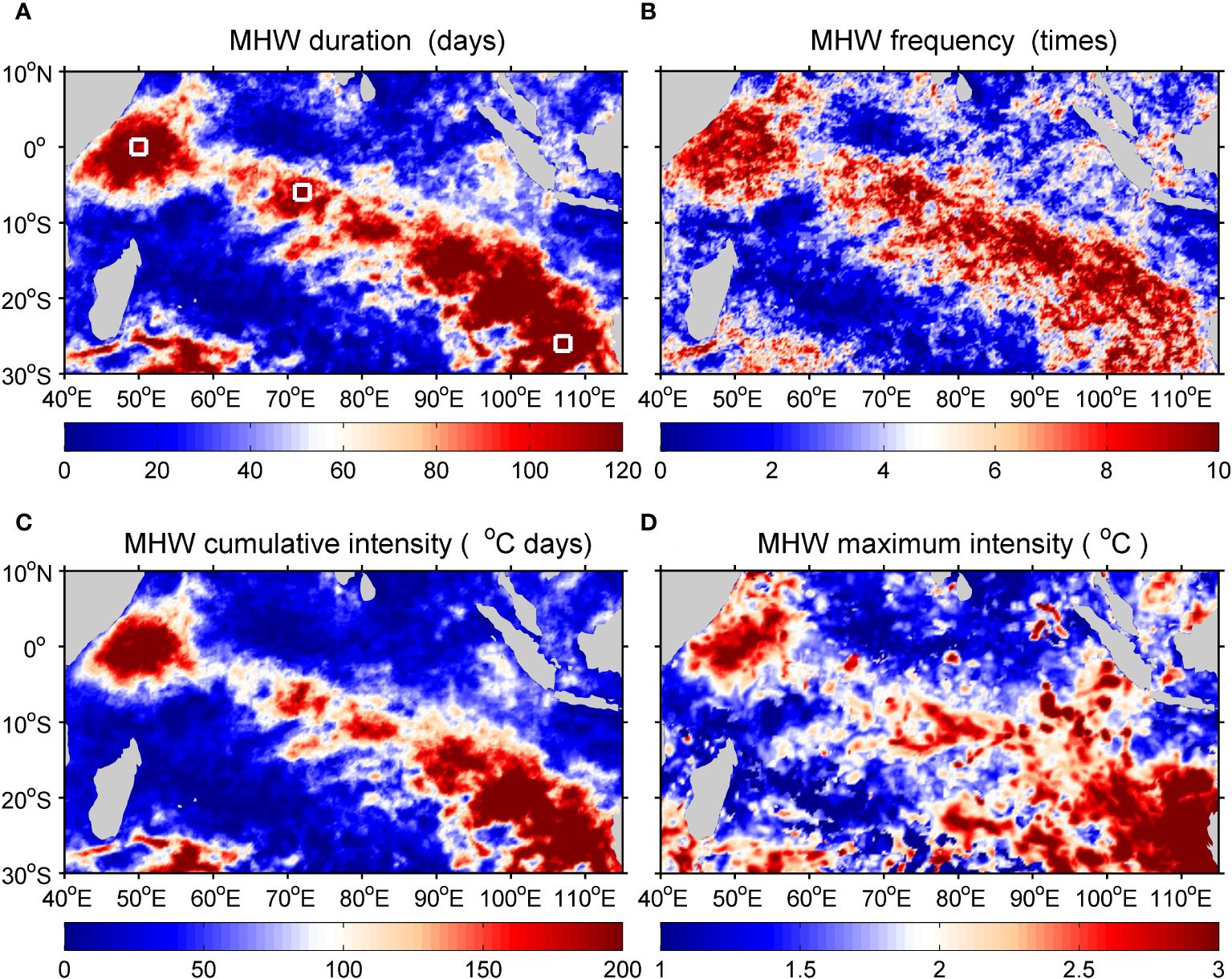
Figure 1 Spatial patterns of MHW metrics in the TIO for 2012: (A) duration, (B) frequency, (C) cumulative intensity, and (D) maximum intensity. The white squares indicate three 2°2° boxes selected in the western (49–51°E, 1°S–1°N), southwestern (71–73°E, 7–5°S) and southeastern (106–108°E, 27–25°S) TIO, respectively.
The rest of this paper was organized as follows. In Section 2, the data and methods used in this study were described. In Section 3, we used various observational and reanalysis datasets to quantify the triggers of the TIO MHWs and the unseasonable pIOD event during the summer of 2012, and further investigated their broader climatic impacts. In Section 4, the main results were discussed, and a conclusion was provided in section 5.
2 Materials and methods
2.1 Data
We used the 0.25°0.25°, daily and monthly satellite SST data from the National Oceanic and Atmospheric Administration Optimum Interpolation Sea Surface Temperature (OISST) High Resolution Dataset Version 2 (Reynolds et al., 2007) due to its high resolution and comprehensive temporal coverage. The El Niño–Southern Oscillation (ENSO) is characterized by the Oceanic Niño Index (ONI), which is defined as the area–averaged SSTAs over the Niño 3.4 region (170–120°W, 5°S–5°N). The monthly ONI indexes were calculated using the OISST dataset. Daily temperature measured by the Research Moored Array for African–Asian–Australian Monsoon Analysis and Prediction (RAMA) moored buoy (McPhaden et al., 2009) at 8°S, 80.5°E was used. The climatology was derived from the RAMA buoy data during 19 August 2008 to 21 January 2021. We used the 0.25°0.25°, monthly Ocean ReAnalysis System 5 (ORAS5) temperature and D20 products from the European Centre for Medium–Range Weather Forecasts (Zuo et al., 2019). The global, 1°1° monthly temperature gridded Argo dataset from the Grid Point Value of the Monthly Objective Analysis using Argo float data were used (Hosoda et al., 2008). The Argo data have a horizontal resolution of 1°1° and are available from January 2001 to December 2018. We nominally treated the temperature at 10 m (first level) as that from the sea surface.
The monthly atmospheric datasets (sea level pressure, wind speeds at 10 m and pressure level, and pressure velocity) were obtained from the National Centers for Environmental Prediction/National Center for Atmospheric Research (NCEP–NCAR) reanalysis data at a resolution of 2.5°2.5° (Kalnay et al., 1996). The precipitation data were derived from the 2.5°2.5° gridded monthly Global Precipitation Climatology Project version 2.3 dataset (Huffman et al., 2009). We used the monthly 2.5°2.5° National Oceanic and Atmospheric Administration outgoing longwave radiation (OLR) data (Liebmann and Smith, 1996) to estimate the convective activities. The global, 0.25°0.25° sea surface height (SSH) from 1993 to 2022 was provided by the Copernicus Marine and Environment Monitoring Service. The SSH anomalies (SSHAs) were obtained by subtracting the monthly climatology from the data and then removing the long–term trends. Except for the Argo (2001–2018) and SSH (1993–2022), all the data from 1983 to 2022 were used for analysis.
2.2 Identification of unseasonable pIOD events
The Dipole Mode Index (DMI) of the IOD is defined as the SSTAs difference between the western (50–70°E, 10°S–10°N) and eastern (90–110°E, 10°S–equator) poles (Saji et al., 1999). We used the monthly SSTA from the OISST dataset during 1983–2022 to estimate the DMI. Following Du et al. (2013), the monthly DMI was bandpass filtered at 4–84 months to remove the intraseasonal and long–term variations. Then, the bandpass filtered DMI with the value larger (smaller) than one standard deviation was recognized as a positive (negative) IOD event. Finally, IOD events that developed and matured within June–August were identified as unseasonable IOD events. According to these criteria, five unseasonable IOD events were identified during 1983–2022: 1983, 2003, 2007, 2008 and 2012. In particular, the 2012 event abruptly developed in July and peaked in August (Figure 2), which ranked as the strongest one among these five unseasonable pIOD events.
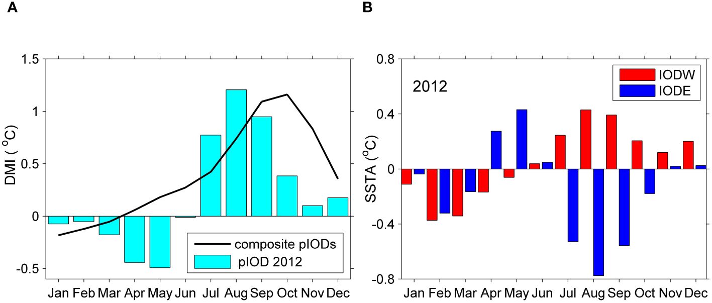
Figure 2 (A) Monthly evolution of the DMI for pIOD 2012 (bars) and composite pIODs (line). In the composite analysis, the pIOD years were 1994, 1997, 2006, 2015 and 2019 according to the Australian government Bureau of Meteorology. (B) SSTA averaged over the IODW (50–70°E, 10°S–10°E) and IODE (90–110°E, 10°S–equator) for 2012. Note that the DMI, IODW and IODE were bandpass filtered at 4–84 months to remove the intraseasonal and long–term variations according to Du et al. (2013).
2.3 Definition of MHWs
Following Hobday et al. (2016), a MHW is defined as a discrete anomalously warm event in which the SST is above the 90th percentile threshold based on the 40–year climatological daily mean and persists for more than five days. A set of specific metrics is used to characterize the MHWs, such as the duration (the time period between the start and end dates of a MHW event), frequency (the number of all MHW events in a year), cumulative intensity (sum of temperature anomalies during a MHW event), and maximum intensity (maximum temperature anomaly during a MHW event). In this study, we used the daily OISST data from 1983 to 2022 to estimate the MHWs at each grid point. Along with the annual values, we also estimated the MHW metrics from June to September (JJAS) of 2012.
2.4 SST products intercomparison/validation
To validate the data accuracy, we made a comparison between the OISST, Argo and ORAS5 SST. The annual mean SST from the OISST, Argo, and ORAS5 datasets show similar spatial distributions (Figures 3A–C). High SST occurs in the northern Indian Ocean except for the Somalia coast and northwest Arabian Sea, where local upwelling causes cold SST. To quantify the comparison, the time series of monthly SST and the anomaly averaged over the TIO (40–110°E, 20°S–20°N) are shown. Both the SST and SSTA from the Argo and ORAS5 area–averaged over the TIO compare well with those from the OISST dataset. The correlation coefficient of SST between the Argo and OISST is 0.98, and the root mean square error (RMSE) is 0.17°C. The correlation coefficient of SST between the ORAS5 and OISST is 0.99, and the RMSE is 0.15°C (Figure 3D). The correlation coefficient of SSTA between the Argo and OISST is 0.88, and the RMSE is 0.26°C. The correlation coefficient of SSTA between the ORAS5 and OISST is 0.93, and the RMSE is 0.15°C (Figure 3E). Overall, the comparison confirms good agreements between the three datasets. The ORAS5 dataset shows better agreement with the OISST dataset. We then used the three–dimensional ORAS5 and Argo datasets to characterize the vertical structure of MHWs in the TIO.
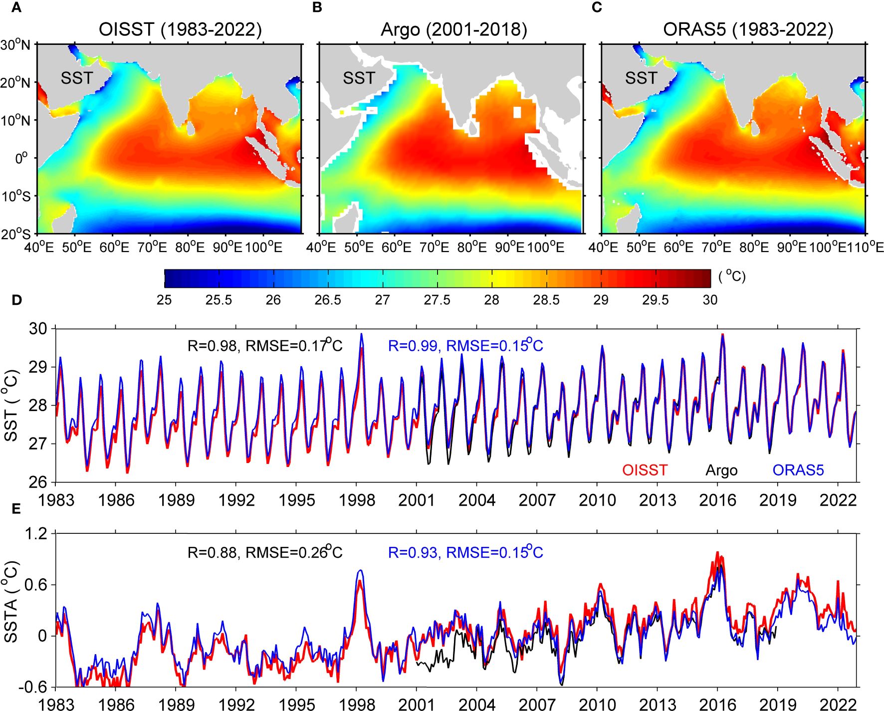
Figure 3 Annual mean SST for the OISST (A), Argo (B) and ORAS5 (C) datasets. Comparison of SST (D) and SSTA (E) averaged over the TIO (40–110°E, 20°S–20°N) from the OISST (red), Argo (black) and ORAS5 (blue) datasets. The correlation coefficient and RMSE between the time series of the two datasets are labeled in the panel.
3 Results
3.1 MHWs in the TIO during the summer of 2012
Several recent studies have reported the MHWs in the Arabian Sea (Chatterjee et al., 2022), Bay of Bengal (Lin et al., 2023) and EIO (Zhang et al., 2021; Qi et al., 2022; Saranya et al., 2022). Based on the definition of Hobday et al. (2016), we estimated the MHW metrics (duration, frequency, cumulative intensity and maximum intensity) in the TIO. In 2012, intense MHWs occurred in the TIO with the duration, frequency, cumulative intensity and maximum intensity featured northwestward–slanted patterns from west Australia to the Somalia coast (Figure 1). The spatial patterns of the MHW metrics showed that the 2012 MHWs occurred primarily in three subregions: the southeastern (SETIO), southwestern (SWTIO) and WTIO. We selected three 2°2° boxes in the SETIO (106–108°E, 27–25°S), SWTIO (71–73°E, 7–5°S) and WTIO (49–51°E, 1°S–1°N). The daily SST averaged over the three boxes was used to analyze the temporal variations in local MHWs (Figure 4). The time series of daily SST suggested that the SETIO was almost in a continuous MHW state from February to July of 2012, largely influenced by the preceding La Niña event (Benthuysen et al., 2014). According to the MHW metrics, this event had a duration of 159 days (with a gap of two days), a maximum intensity of 2.9°C and a cumulative intensity of 240°C days. The spatial pattern of the weekly SSTA indicated that this MHW event can be attributed to the 2011–2012 La Niña (Feng et al., 2013; Xu et al., 2018). In contrast, the MHWs in the SWTIO and WTIO were periodic over several weeks. This suggested that oceanic waves may have played an important role. The time series of daily SST confirmed that prominent MHWs in the SWTIO and WTIO persisted from the summer to winter of 2012. Considering that the unseasonable pIOD 2012 peaked in summer and that this event may be an important trigger of these MHWs, we primarily focused on the anomalies during the summer of 2012.
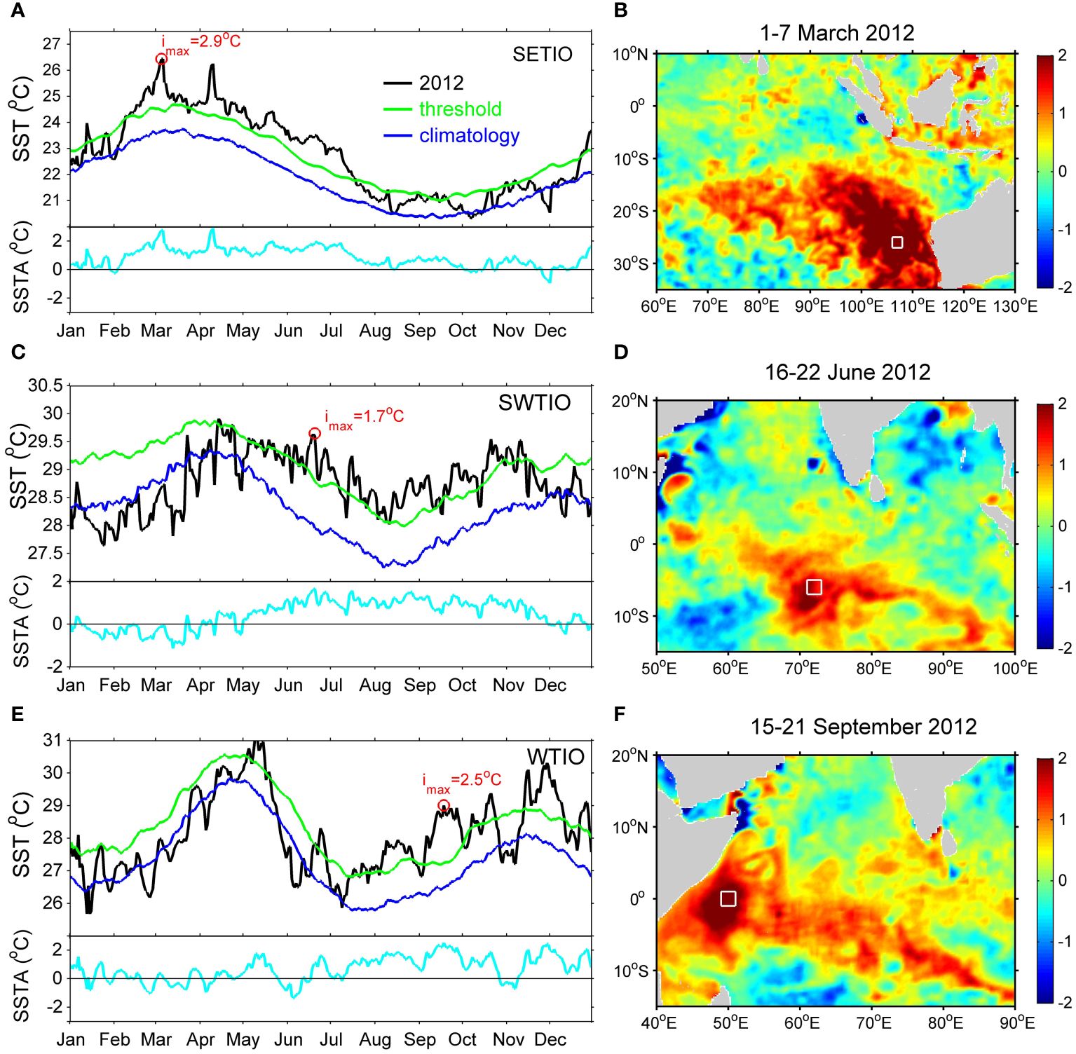
Figure 4 Seasonally varying MHWs in the three representative boxes in the SETIO (A), SWTIO (C), and WTIO (E). In the varying MHWs, the curves correspond to the SST (black), the 90th percentile seasonally varying threshold (green), the climatology (blue) and SSTA (cyan). The maximum intensity of the MHWs is labeled in each panel. Spatial patterns of weekly SSTA when the intensity reaches the maximum in the SETIO (B), SWTIO (D, F) WTIO. The white squares indicate the three 2°2° boxes in the SETIO (106–108°E, 27–25°S), SWTIO (71–73°E, 7–5°S) and WTIO (49–51°E, 1°S–1°N).
The spatial patterns of MHW duration and cumulative intensity in the TIO during JJAS of 2012 were shown in Figure 5. The northwestward–slanted patterns of the MHW metrics can still be found, especially in the SWTIO and WTIO. The JJAS SSTA showed positive values extending northwestward from west Australia to the Somalia coast and negative values occurring in the northwest Australia and eastern TIO. The spatial pattern of the ORAS5 SSTA showed good agreement with that of the OISST data (Figures 5C, D). This motivated us to use the three–dimensional ORAS5 data to further examine the vertical structure of the MHWs in the TIO during the summer of 2012.
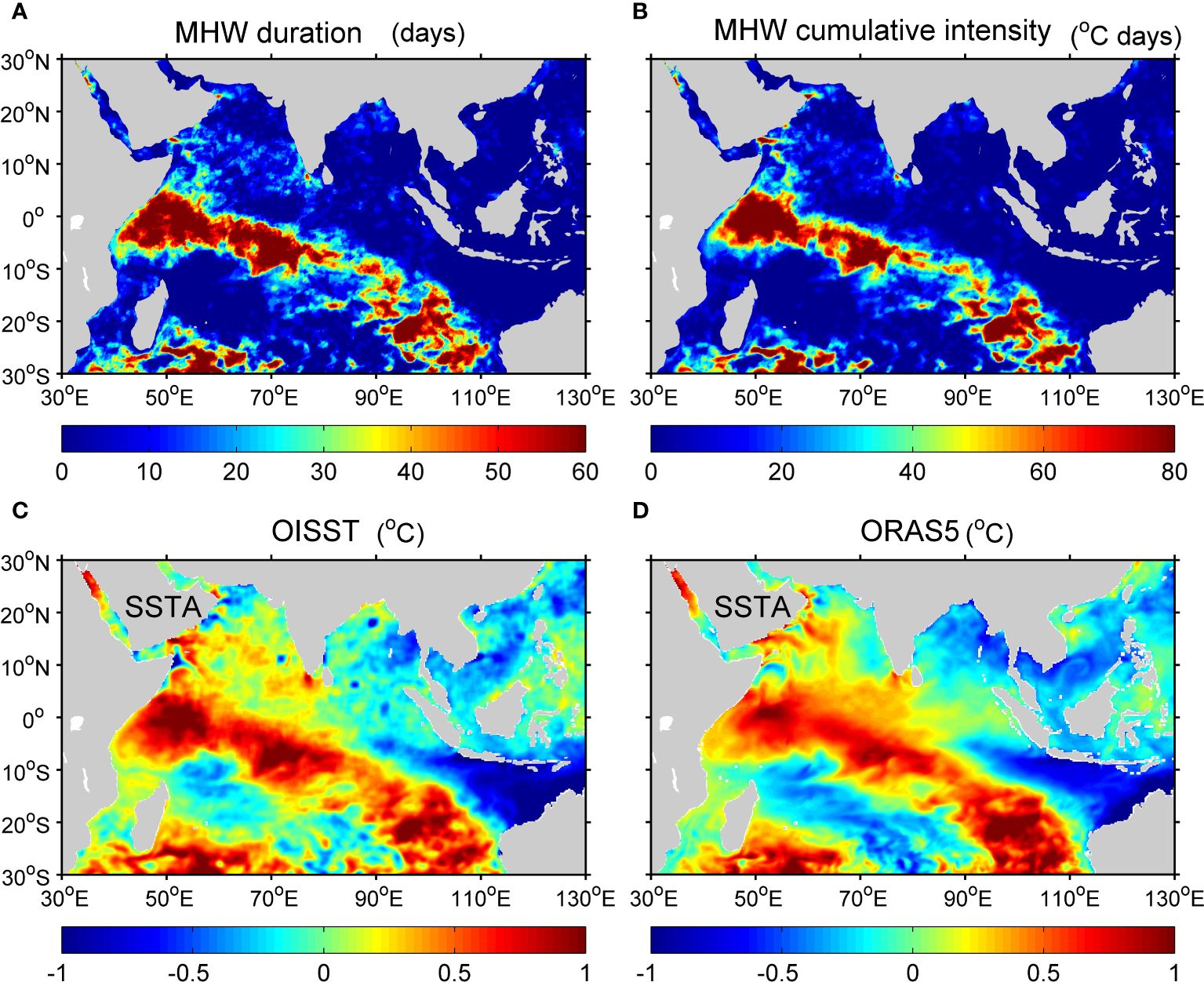
Figure 5 Spatial patterns of the MHW metrics (A: duration; B: cumulative intensity) and SSTA (C: OISST; D: ORAS5) averaged from June to September of 2012.
Considering that intense summer MHWs occurred primarily in the WTIO and SWTIO, we used two 2°2° boxes to represent the two regions. Figure 6 shows the depth–time plots of the temperature anomaly area–averaged over the WTIO (49–51°E, 1°S–1°N) and the SWTIO (71–73°E, 7–5°S) based on the ORAS5 and Argo datasets. The evolution of the temperature anomaly and thermocline depth (depth of 20°C isotherm, D20) of the two datasets showed consistent features: significant and sustained thermocline deepening and subsurface warming were noted in the two regions during the summer of 2012. Thus, the thermocline deepening caused anomalously warm SSTAs, as suggested by Xie et al. (2002) and Zhang et al. (2021). This indicated that the MHWs in the SWTIO and WTIO were related to the thermocline deepening. The RAMA buoy positioned at 8°S, 80.5°E is located in the SWTIO region. Therefore, the RAMA data provide insights into the oceanic variability associated with the MHWs in 2012. Figure 6E shows the depth–time plot of the daily temperature observed from the RAMA buoy at 8°S, 80.5°E. The temperature exhibited a downward displacement of the thermocline (D20) from June to September of 2012. The thermocline deepened from less than 60 m to more than 170 m during this period. Climatologically, the thermocline deepens from approximately 60 m to 118 m during JJAS. Yokoi et al. (2008) showed that the seasonal variation of the thermocline depth in the SWTIO was due to local Ekman pumping. These results indicated that the interannual variability of the D20 was more than 60 m during JJAS of 2012. This suggested that anomalous downwelling processes occurred in the SWTIO and WTIO during the summer of 2012.
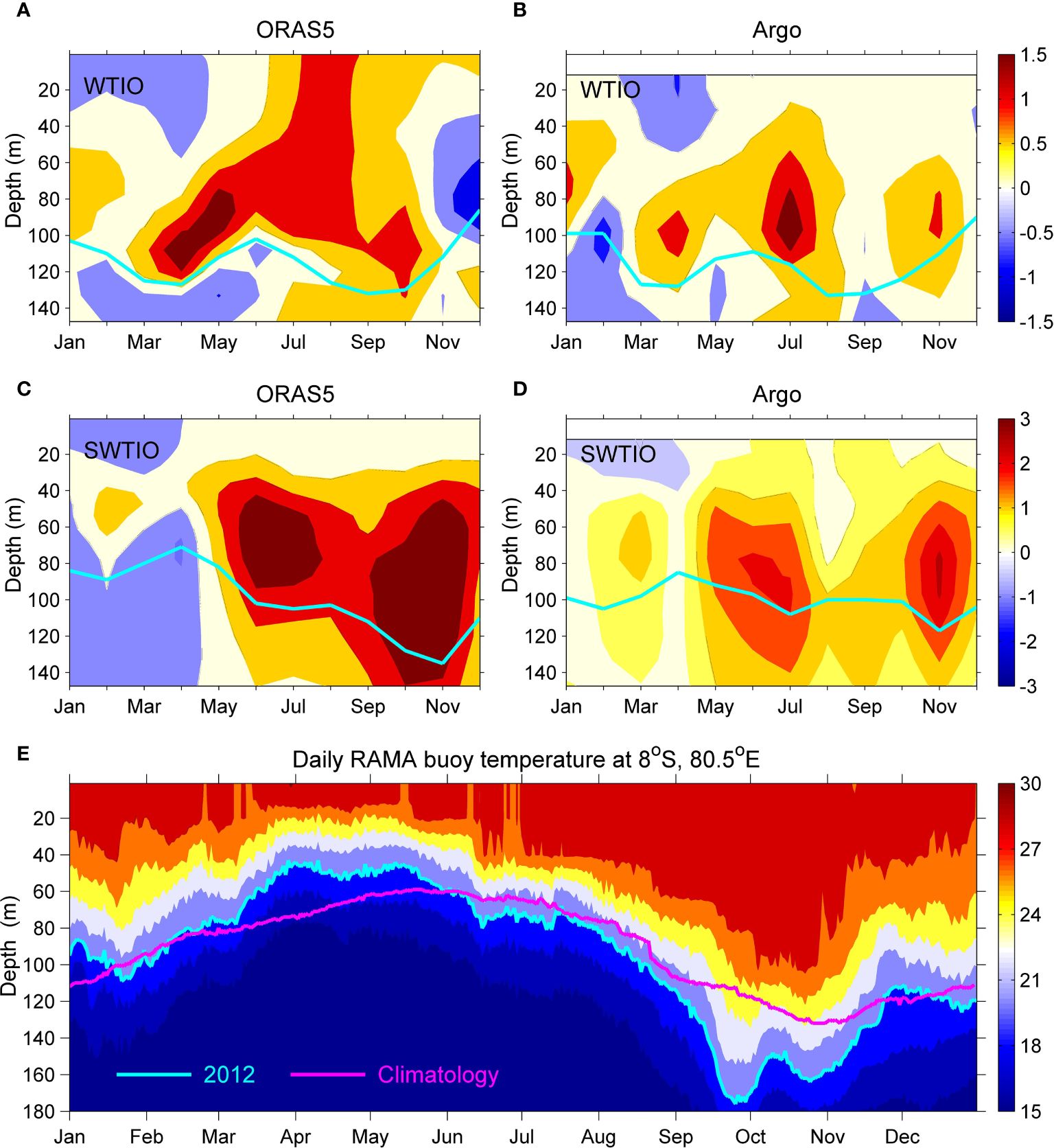
Figure 6 Depth–time plots of potential temperature anomalies (color, °C) averaged over the WTIO (A, B) and the SWTIO (C, D) in 2012 based on the Argo and ORAS5 datasets. The cyan line indicates the contour of D20 (depth of 20°C isotherm). (E) Depth–time evolution of the daily temperature (color, °C) in 2012 overlapped with D20 (contour, m) observed from the RAMA buoy at 8°S, 80.5°E. The purple line represents the climatology of D20 based on the daily RAMA buoy temperature from 19 August 2008 to 21 January 2021.
3.2 An unseasonable pIOD 2012
The SSTA clearly exhibited a zonal dipole pattern in the TIO with warm in the west and cold in the east, suggesting a pIOD event during the summer of 2012 (Figure 5C). The DMI estimated from the OISST dataset showed that a pIOD event developed abruptly and peaked during the July–September (JAS) of 2012 (Figure 2A). Compared with the canonical pIOD events that mature in SON, pIOD 2012 was an unseasonable IOD event according to the classification of Du et al. (2013). During the peak phase of this event, significant negative SSTAs (upwelling) occurred in the eastern pole and positive SSTAs (downwelling) occurred in the western pole (Figure 2B).
To characterize these upwelling and downwelling processes, the SSHAs in the TIO averaged during the JAS of 2012 were shown in Figure 7. Significant negative SSHAs associated with upwelling occurred in the eastern EIO (Figure 7A), and positive SSHAs associated with downwelling appeared in the western EIO, reflecting the mature phase of the pIOD event (Du et al., 2020; Lu and Ren, 2020; Li et al., 2021). In addition, a band of positive SSHAs extending from the SETIO to the SWTIO was particularly noticeable. Figure 7B shows the longitude–time plot of SSHAs averaged over 12–8°S in the TIO in 2012. It clearly showed downwelling Rossby waves propagating westward from the SETIO to the thermocline dome, which was in agreements with the findings of previous studies (Xie et al., 2002; Rao and Behera, 2005; Yu et al., 2005). Therefore, with the development of the pIOD 2012, westward–propagating downwelling Rossby waves deepened the thermocline and caused anomalous surface warming in the MHW regions.
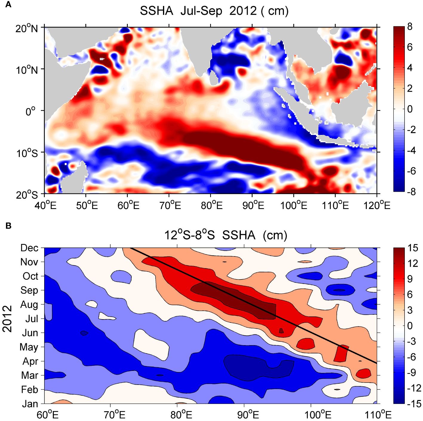
Figure 7 (A) Spatial patterns of SSHAs in the TIO averaged from the July to September (JAS) of 2012. (B) Longitude–time plot of SSHAs averaged over 12–8°S in the TIO in 2012. The black line indicates the westward propagation of the downwelling Rossby waves.
The above analysis confirmed that the summer MHWs in the TIO were associated with the unseasonable pIOD 2012. Therefore, it is necessary to figure out how this unusual pIOD event was triggered. Previous studies concluded that an IOD event can be triggered by air–sea coupling processes during the boreal spring (Annamalai et al., 2003; Li et al., 2003; Fischer et al., 2005), anomalous anticyclonic wind circulation over the SETIO (Yu et al., 2005), or an interhemispheric pressure gradient (IHPG) over the eastern TIO (Lu and Ren, 2020). We examined the atmospheric forcing conditions one season earlier than the peak phase of pIOD 2012. Figure 8 shows the anomalies of sea level pressure (SLP) and 10 m wind during the April–May of 2012. The SLP clearly showed positive anomalies extending northwestward from Australia to the Arabian Sea and negative anomalies appearing in the Bay of Bengal, Maritime Continent and the South China Sea (Figure 8A). This suggested a weakening of the Western North Pacific Subtropical High (WHPSH) and a strengthening of the Australian High (AH) (Watanabe and Jin, 2002; Sandaruwan et al., 2023). The asymmetric pressure anomaly over the two hemispheres generated an IHPG that contributed to two anticyclonic wind anomalies over the eastern TIO. The first anticyclonic anomaly was characterized by cross–equatorial anomalies over the two hemispheres, with winds blowing from south of Java to the South China Sea/Philippine Sea (SCS/PS) through the Bay of Bengal. The second anticyclonic anomaly was observed in the SETIO and was characterized by winds blowing from south of Java to the west Australia.
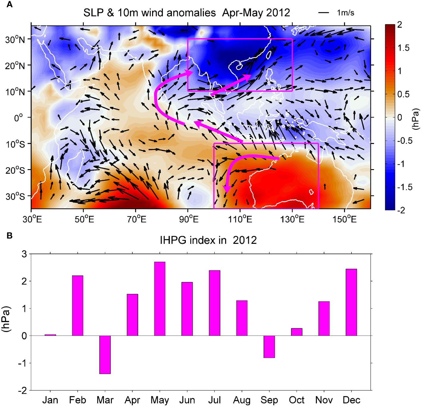
Figure 8 (A) Spatial patterns of the anomalies of SLP (shading) and 10 m wind (vectors) during the April–May of 2012. The two purple boxes indicate the regions (100–140°E, 35–10°S; 90–130°E, 10–30°N) used to estimate the interhemispheric pressure gradient (IHPG) index. The purple arrows indicate the anticyclonic wind anomalies in the SETIO and cross–equatorial wind anomalies from eastern EIO to the South China Sea/Philippine Sea through the Bay of Bengal. The vector with a wind speed of less than 0.5 m/s is not plotted. (B) Evolution of the IHPG index defined as the SLP anomaly difference between (100–140°E, 35–10°S) and (90–130°E, 10–30°N).
An IHPG index was defined as the SLP anomaly difference between Australia (100–140°E, 35–10°S) and the South China Sea as well as the adjacent regions (90–130°E, 10–30°N) to measure the strength of the meridional pressure gradient (Lu and Ren, 2020). The IHPG index was positive in April and remained positive until August 2012 (Figure 8B). This suggested that the IHPG played an important role in initiating the pIOD 2012, which was interpreted as follows. First, the upwelling–favorable winds (associated with the cross–equatorial wind anomalies) led to a thermodynamical air–sea feedback that strengthened the upwelling off Sumatra–Java during the subsequent summer (Li et al., 2003). Second, anticyclonic anomalies in the SETIO excited downwelling Rossby waves as a Matsuno–Gill response (Fischer et al., 2005; Yu et al., 2005). These downwelling Rossby waves propagated westward along 12–8°S to the SWTIO (Figure 7), deepening the thermocline and causing warm SSTAs during the following summer. These results were in agreements with the findings of Rao and Behera (2005) and Xie et al. (2002). As a result, downwelling in the west and upwelling in the east led to a pIOD event peaking in summer, one season earlier than the canonical IODs. We concluded that the IHPG over the eastern TIO in spring was the key to triggering the unseasonable pIOD 2012.
3.3 Implications on the summer monsoon rainfall
Having established the characteristics of the MHWs and the role of the unseasonable pIOD 2012, we now examine the broader implications on summer monsoon rainfall patterns over adjacent regions. To achieve this, we analyzed the anomalies of wind at pressure level, pressure velocity (omega), OLR and precipitation during the JJAS of 2012 (Figure 9). From an overall view, the lower level (700 hPa winds) atmospheric circulation showed a clockwise pattern over the TIO and northern Indian subcontinent and featured a counterclockwise pattern in the subtropical western North Pacific (WNP). We selected the winds at 700 hPa to represent the lower level atmospheric circulation because the wind speeds at this level were higher than those at 850, 925, and 1000 hPa (Figure 9B). Regionally, easterly anomalies blew from the SETIO to the WTIO and then turned southwesterly to the Arabian Sea, indicating strengthening of the South Asian Summer Monsoon. When it reached the northern Indian subcontinent, the southwesterly anomalies shifted northwesterly toward the Maritime Continent via the Bay of Bengal. The wind anomalies formed a strong cyclonic pattern over the SCS/PS. The JJAS OLR anomaly exhibited striking regional features over the TIO, Indian subcontinent, and subtropical WNP. Positive OLR anomalies occurred in Australia, SETIO, and the eastern EIO, indicating suppressed convection over these regions. Negative OLR anomalies (enhanced convection) occurred in the MHWs regions, northern Indian subcontinent, Bay of Bengal, and subtropical WNP. In the following section, we further explored the dominant air–sea processes associated with these anomalies.
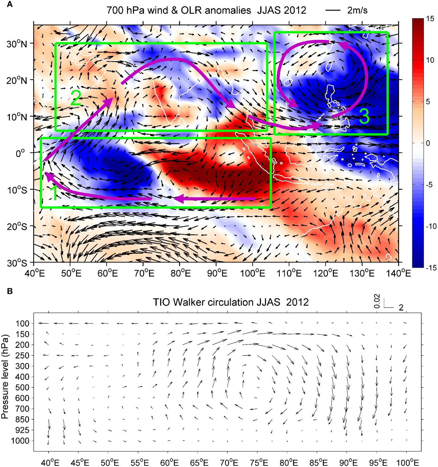
Figure 9 (A) Anomalies of 700 hPa wind (vectors; m/s) and OLR (shading; W/m2) in the TIO and subtropical WNP. (B) Longitude–pressure anomalies of zonal wind (m/s) and vertical pressure velocity (omega, Pa/s) averaged between 15°S–5°N. All the anomalies were averaged from the June to September of 2012. The bold purple arrows indicate the schematic of atmospheric circulation, and the green boxes indicate three regions of different air–sea processes.
Three regions involving different air–sea processes were identified based on the spatial patterns of the OLR and wind anomalies. The first region was the EIO and the area adjacent to the south (box 1 in Figure 9A). The second region included the Arabian Sea, Bay of Bengal, and the Indian subcontinent (box 2 in Figure 9A). The third region was the subtropical WNP (box 3 in Figure 9A). In the first region, the wind and OLR anomalies primarily reflected the Walker circulation in the TIO associated with the pIOD 2012 (Figure 9B). The TIO Walker circulation associated with pIOD 2012 was characterized by an ascending/descending branch over the western/eastern EIO and easterly anomalies at the lower level (Figure 9B) (Du et al., 2020). Therefore, the Indonesian region and eastern EIO suffered from below normal rainfall, and the MHWs regions received above normal rainfall (Figure 10). This was consistent with the findings of previous studies (Cai et al., 2014; Zhang et al., 2018; Lu and Ren, 2020; Li et al., 2021, 2023).
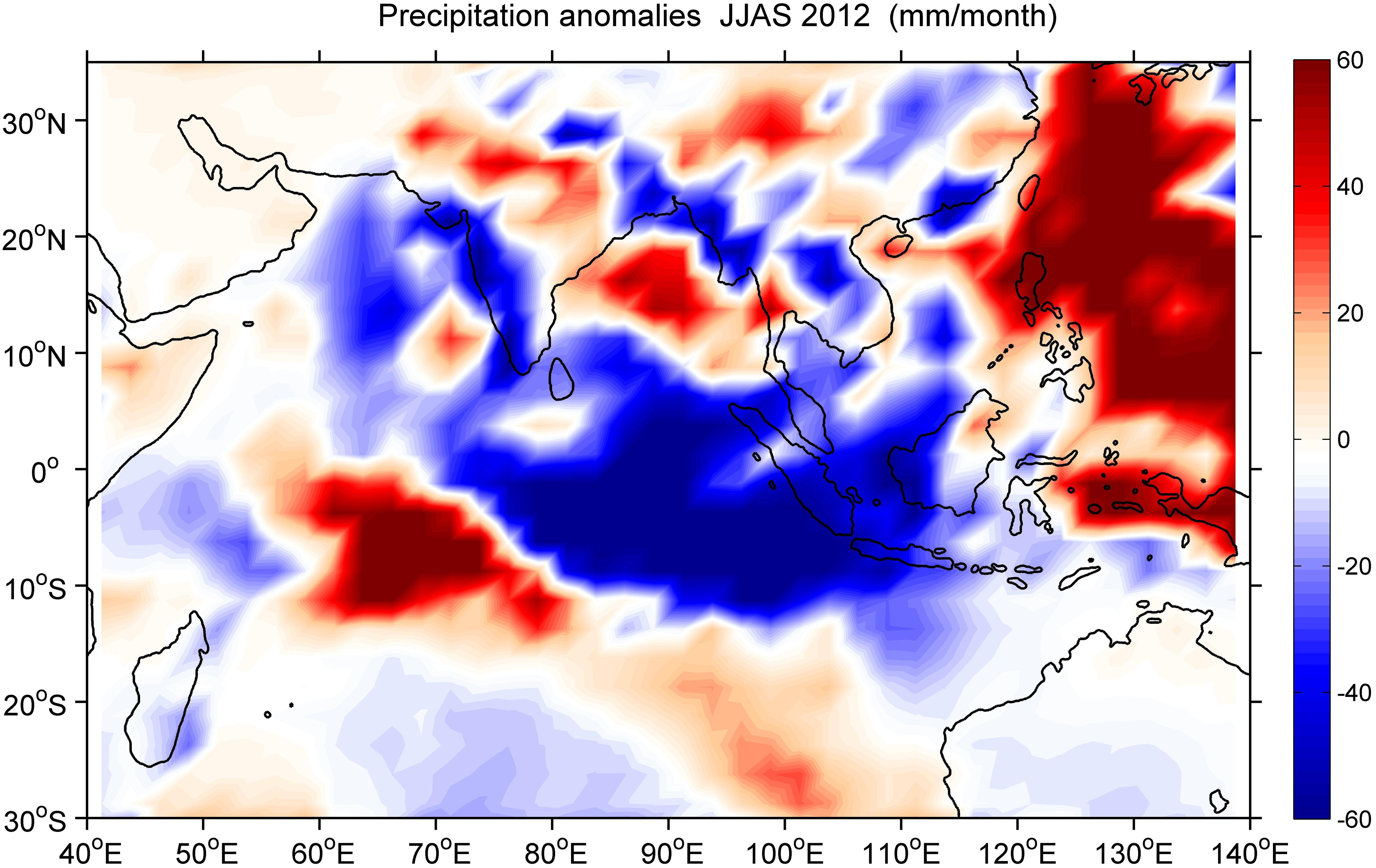
Figure 10 Spatial pattern of precipitation anomalies during the June–September of 2012.
In the second region, the wind and OLR anomalies suggested that the strengthened South Asian Summer Monsoon transported moisture from the WTIO to land. The ascending motion of the moisture (enhanced convection) caused above normal rainfall over the northern Indian subcontinent and Bay of Bengal (Figure 10). These results were consistent with the findings in several studies (Behera et al., 1999; Ashok et al., 2001; Ratna et al., 2021). In the third region, the wind and OLR anomalies indicated that the northwesterly wind from the Bay of Bengal contributed to a strong cyclonic anomaly accompanied by enhanced convection over the subtropical WNP. Therefore, above normal rainfall occurred in the Philippine Sea and surrounding regions (Figure 10). The above analysis confirmed that the unseasonable pIOD 2012 favored an anomalous atmospheric circulation that transported moisture from TIO to the subtropical WNP via the Indian subcontinent (Figure 9A). The strong cyclonic anomaly and the ascending motion of moisture led to above normal rainfall over the subtropical WNP (Figure 10). As part of the unseasonable pIOD 2012, the summer MHWs (high SST) favored the ascending motion of moisture and enhanced convection, which was a key connection between moisture transport in the TIO and subtropical WNP. In summary, the summer of 2012 saw intense MHWs in the TIO driven by an unseasonable pIOD event. This unseasonable pIOD event not only influenced the MHWs but also had significant impacts on regional climate, particularly the summer monsoon rainfall in the subtropical WNP.
4 Discussion
Unusual IOD events have increased under global warming in recent decades (Cai et al., 2009, 2014; Li et al., 2021), leading to various types and triggers of IOD (Du et al., 2013; Guo et al., 2015). Du et al. (2013) classified IOD events into different types based on their peak seasons and proposed a new type that matures in summer, namely, the unseasonable IOD. Du et al. (2013) attributed the trigger of unseasonable IOD events to equatorial wind changes related to the weakening Walker circulation in the TIO. They concluded that the unseasonable IOD events were an intrinsic mode of the Indian Ocean, independent of ENSO in the Pacific. In this study, the pIOD 2012 was recognized as an unseasonable IOD event according to the classification of Du et al. (2013). The DMI of this event reached to 1.1°C, belonging to a strong pIOD year according to the Australian government Bureau of Meteorology (http://www.bom.gov.au/climate/iod/). However, to date, there has been relatively few research conducted on the pIOD 2012 (Tanizaki et al., 2017). Our results differed from those of Du et al. (2013) in terms of the trigger of unseasonable IOD events. We found that the unseasonable pIOD 2012 was triggered by an IHPG over the eastern TIO during spring (Figure 8). This was in agreement with the findings of Lu and Ren (2020) and Sandaruwan et al. (2023) that the IHPG is a key trigger of IOD events. We found that a modest El Niño event developed during the JJAS of 2012, after the consecutive La Niña events of 2010–2011 (Figure 11A). The SSTA pattern further confirmed that pIOD 2012 co–occurred with El Niño in the Pacific (Figure 11B). This indicated that the unseasonable pIOD 2012 was likely dependent on the concurrent El Niño in the Pacific. This is because ENSO is a well–known trigger of IOD events (Saji and Yamagata, 2003; Behera et al., 2006; Zhang et al., 2015; Stuecker et al., 2017; Cai et al., 2019).
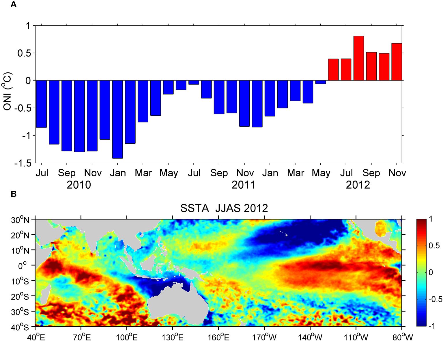
Figure 11 (A) Monthly evolution of ONI from 2010 to 2012 based on the OISST dataset. The blue bars represent the La Niña events 2010–2011 and the red bars indicate the modest El Niño in 2012. (B) Spatial pattern of SSTA (°C) in the Indian Ocean and Pacific averaged during the JJAS of 2012.
Strong downwelling Rossby waves associated the unseasonable pIOD 2012 propagated northwestward from SETIO to the thermocline dome (Figure 7). These anomalous downwelling waves deepened the thermocline by more than 60 m, which was comparable with the seasonal variation of the D20 (Yokoi et al., 2008). These downwelling waves caused anomalous surface warming, thereby contributing to the occurrences of MHWs over the western and southwestern TIO (Figure 6). Consequently, we argued that the unseasonable pIOD 2012 was responsible for the summer MHWs in the TIO. These results support the findings in several recent studies that downwelling processes were important triggers of MHWs in TIO during pIOD years (Zhang et al., 2021; Qi et al., 2022; Sandaruwan et al., 2023). While the present study provides new insights into the triggers of MHWs and pIOD events during the summer of 2012, it is limited by the resolution of available datasets. Future research should focus on long–term monitoring of MHWs and pIOD events, utilizing high–resolution observational data and advanced modeling techniques to improve predictive capabilities.
With the development and peak of the unseasonable pIOD 2012, a strong cyclonic anomaly accompanied by enhanced convection and heavy precipitation occurred over the subtropical WNP (Figures 9, 10). The wind and OLR anomalies indicated that anomalous atmospheric circulation associated with the unseasonable pIOD 2012 transported moisture from TIO to the subtropical WNP. The strong cyclonic anomaly and the ascending motion of moisture contributed to heavy summer rainfall over the subtropical WNP (Figure 9A). Therefore, the unseasonable pIOD 2012 profoundly affected summer monsoon rainfall over subtropical WNP. This is in agreement with the findings of Annamalai et al. (2005). As part of the unseasonable pIOD 2012, the summer MHWs favored the ascending motion of moisture. This was crucial for connecting the moisture transport between TIO and the subtropical WNP. In particular, the strong cyclonic anomaly and heavy summer rainfall over the SCS/PS can significantly influence the East Asian Summer Monsoon via atmospheric teleconnection (Kubota et al., 2015; Xie et al., 2016). Further studies are needed to investigate the role of the unseasonable pIOD 2012 in summer climate over the Indo–Northwest Pacific region.
5 Conclusion
The TIO has experienced the most significant surface warming since mid–1970s (Du and Xie, 2008). This has led to an increase in duration, frequency and intensity of MHWs in recent years (Zhang et al., 2021; Sandaruwan et al., 2023). The MHWs in the TIO exhibited evident interannual variability, which was attributed to the IOD events (Chatterjee et al., 2022; Saranya et al., 2022; Lin et al., 2023; Sandaruwan et al., 2023). During the summer of 2012, intense MHWs occurred in the TIO concurrently with an unseasonable pIOD event. By analyzing various reanalysis and observational datasets, the triggers of the summer TIO MHWs and the unseasonable pIOD 2012 as well as their broader climatic impacts were investigated.
The results show that the unseasonable pIOD 2012 was triggered by an IHPG over the eastern TIO. During the spring of 2012, the atmospheric circulation was characterized by a weakening of the WNPSH and a strengthening of the AH. Therefore, an IHPG formed over the two hemispheres, which drove two anticyclonic circulation patterns over the eastern TIO. The first anticyclonic circulation featured cross–equatorial wind anomalies from south of Java to the SCS/PS via the Bay of Bengal. These cross–equatorial wind anomalies led to a thermodynamical air–sea feedback that strengthened the upwelling off Sumatra–Java during the subsequent summer. The second anticyclonic circulation excited downwelling Rossby waves that propagated northwestward from SETIO to the thermocline dome. As a result, downwelling in the western pole and upwelling in the eastern pole contributed to the peak of a strong pIOD event in summer, namely, the unseasonable pIOD 2012. These downwelling waves associated with the pIOD 2012 deepened the thermocline by more than 60 m and caused anomalous surface warming, thereby contributing to the occurrences of MHWs over the western and southwestern TIO. Therefore, we conclude that the unseasonable pIOD 2012 was responsible for the summer MHWs in the TIO. Moreover, the unseasonable pIOD 2012 caused anomalous moisture transport from the TIO to the WNP, favoring strong cyclonic anomalies over the subtropical regions. This, in turn, led to above normal summer monsoon rainfall in the subtropical WNP. This study provides new insights into the mechanisms driving the TIO MHWs and unseasonable pIOD events, contributing to a better understanding of regional climate variability and its ecological consequences.
Data availability statement
The original contributions presented in the study are included in the article/supplementary material. Further inquiries can be directed to the corresponding author.
Author contributions
ZL: Conceptualization, Visualization, Writing – original draft, Writing – review & editing. GW: Conceptualization, Data curation, Formal analysis, Methodology, Writing – review & editing. CX: Data curation, Formal analysis, Investigation, Software, Writing – review & editing. X-HZ: Conceptualization, Supervision, Visualization, Writing – original draft, Writing – review & editing. YL: Formal analysis, Funding acquisition, Investigation, Methodology, Software, Writing – review & editing.
Funding
The author(s) declare financial support was received for the research, authorship, and/or publication of this article. This work was supported by the Natural Science Foundation of Zhejiang Province (LQ24D060008), the National Natural Science Foundation of China (41920104006), the Scientific Research Fund of the Second Institute of Oceanography, MNR (Grant JZ2001), the Innovation Group Project of the Southern Marine Science and Engineering Guangdong Laboratory, Zhuhai (No. 311020004), the National Natural Science Foundation of China (42106035), the Scientific Research Fund of the Second Institute of Oceanography, MNR (Grant JG2306).
Conflict of interest
The authors declare that the research was conducted in the absence of any commercial or financial relationships that could be construed as a potential conflict of interest.
Publisher’s note
All claims expressed in this article are solely those of the authors and do not necessarily represent those of their affiliated organizations, or those of the publisher, the editors and the reviewers. Any product that may be evaluated in this article, or claim that may be made by its manufacturer, is not guaranteed or endorsed by the publisher.
References
Amaya D., Miller A., Xie S., Kosaka Y. (2020). Physical drivers of the summer 2019 North Pacific marine heatwave. Nat. Commun. 11, 1903. doi: 10.1038/s41467-020-15820-w
Annamalai H., Liu P., Xie S. (2005). Southwest Indian Ocean SST variability: its local effect and remote influence on Asian monsoons. J. Climate 18, 4150–4167. doi: 10.1175/JCLI3533.1
Annamalai H., Murtugudde R., Potemra J., Xie S., Liu P., Wang B. (2003). Coupled dynamics over the Indian Ocean: Spring initiation of the zonal mode. Deep-Sea Res. Part II , 50, 2305–2330. doi: 10.1016/S0967-0645(03)00058-4
Ashok K., Guan Z., Yamagata T. (2001). Impact of the Indian Ocean Dipole on the decadal relationship between the Indian monsoon rainfall and ENSO. Geophys. Res. Lett. 28, 4499–4502. doi: 10.1029/2001GL013294
Behera S., Krishnan R., Yamagata T. (1999). Unusual ocean-atmosphere conditions in the tropical Indian Ocean during 1994. Geophys. Res. Lett. 26, 3001–3004. doi: 10.1029/1999GL010434
Behera S., Luo J., Masson S., Rao S., Sakuma H., Yamagata T. (2006). A CGCM study on the interaction between IOD and ENSO. J. Climate 19, 1608–1705. doi: 10.1175/JCLI3797.1
Benthuysen J., Feng M., Zhong L. (2014). Spatial patterns of warming off Western Australia during the 2011 Ningaloo Niño: Quantifying impacts of remote and local forcing. Continent. Shelf Res. 91, 232–246. doi: 10.1016/j.csr.2014.09.014
Bond N., Cronin M., Freeland H., Mantua N. (2015). Causes and impacts of the 2014 warm anomaly in the NE Pacific. Geophys. Res. Lett. 42, 3414–3420. doi: 10.1002/2015GL063306
Cai W., Pan A., Roemmich D., Cowan T., Guo X. (2009). Argo profiles a rare occurrence of three consecutive positive Indian Ocean Dipole events 2006–2008. Geophys. Res. Lett. 36, L08701. doi: 10.1029/2008GL037038
Cai W., Santoso A., Wang G., Weller E., Wu L., Ashok K., et al. (2014). Increased frequency of extreme Indian Ocean Dipole events due to greenhouse warming. Nature 510, 254–258. doi: 10.1038/nature13327
Cai W., Wu L., Lengaigne M., Li T., McGregor S., Jong-Seong K., et al. (2019). Pantropical climate interactions. Science 363, eaav4236. doi: 10.1126/science.aav4236
Chatterjee A., Anil G., Shenoy L. (2022). Marine heatwaves in the Arabian sea. Ocean Sci. 18, 639–657. doi: 10.5194/os-18-639-2022
Chen K., Gawarkiewicz G., Kwon Y., Zhang W. (2015). The role of atmospheric forcing versus ocean advection during the extreme warming of the Northeast U.S. continental shelf in 2012. J. Geophys. Res.: Oceans 120, 4324–4339. doi: 10.1002/2014JC010547
Chen K., Gawarkiewicz G., Lentz S., Bane J. (2014). Diagnosing the warming of the Northeastern U.S. Coastal Ocean in 2012: A linkage between the atmospheric jet stream variability and ocean response. J. Geophys. Res.: Oceans 119, 218–227. doi: 10.1002/2013JC009393
Di Lorenzo E., Mantua N. (2016). Multi-year persistence of the 2014/15 North Pacific marine heatwave. Nat. Climate Change 6, 1042–1047. doi: 10.1038/nclimate3082
Du Y., Xie S. (2008). Role of atmospheric adjustments in the tropical Indian Ocean warming during the 20th century in climate models. Geophys. Res. Lett. 35, L08712. doi: 10.1029/2008GL033631
Du Y., Cai W., Wu Y. (2013). A new type of the Indian Ocean dipole since the mid–1970s. J. Climate 26, 959–972. doi: 10.1175/JCLI-D-12-00047.1
Du Y., Zhang Y., Zhang L., Tozuka T., Ng B., Cai W. (2020). Thermocline warming induced extreme Indian Ocean dipole in 2019. Geophys. Res. Lett. 47, e2020GL090079. doi: 10.1029/2020GL090079
Feng M., McPhaden M., Xie S., Hafner J. (2013). La Niña forces unprecedented Leeuwin Current warming in 2011. Sci. Rep. 3, 1277. doi: 10.1038/srep01277
Fischer A., Terray P., Guilyardi E., Gualdi S., Delecluse P. (2005). Two independent triggers for the Indian Ocean Dipole/Zonal mode in a coupled GCM. J. Climate 18, 3428–3449. doi: 10.1175/JCLI3478.1
Guo F., Liu Q., Sun S., Yang J. (2015). Three types of Indian Ocean dipoles. J. Climate 28, 3073–3092. doi: 10.1175/JCLI-D-14-00507.1
Hobday A., Alexander L., Perkins S., Smale D., Straub S., Oliver E., et al. (2016). A hierarchical approach to defining marine heatwaves. Prog. Oceanogr. 141, 227–238. doi: 10.1016/j.pocean.2015.12.014
Holbrook N., Scannell H., Gupta A., Benthuysen J., Feng M., Oliver E., et al. (2019). A global assessment of marine heatwaves and their drivers. Nat. Commun. 10, 2624. doi: 10.1038/s41467-019-10206-z
Hosoda S., Ohira T., Nakamura T. (2008). A monthly mean dataset of global oceanic temperature and salinity derived from Argo float observations. JAMSTEC Rep. Res. Dev. 8, 47–59. doi: 10.5918/jamstecr.8.47
Huffman G., Adler R., Bolvin D., Gu G. (2009). Improving the global precipitation record: GPCP Version 2.1. Geophys. Res. Lett. 36, L17808. doi: 10.1029/2009GL040000
Kalnay E., Kanamitsu M., Kistler R., Collins W., Deaven D., Gandin L., et al. (1996). The NCEP/NCAR 40–year reanalysis project. Bull. Am. Meteorol. Soc. 77, 437–471. doi: 10.1175/1520-0477(1996)077<0437:TNYRP>2.0.CO;2
Kubota H., Kosaka Y., Xie S. (2015). A 117–year long indexof the Pacific–Japan pattern with application to interdecadal variability. Int. J. Climatol. 36, 1575–1589. doi: 10.1002/joc.4441
Li J., Liang C., Tang Y., Dong C., Jin W. (2016). A new dipole index of the salinity anomalies of the tropical Indian Ocean. Sci. Rep. 6, 24260. doi: 10.1038/srep24260
Li J., Liang C., Tang Y., Liu X., Lian T., Shen Z., et al. (2018). Impacts of the IOD-associated temperature and salinity anomalies on the intermittent equatorial undercurrent anomalies. Clim. Dyn. 51, 1391–1409. doi: 10.1007/s00382-017-3961-x
Li J., Roughan M., Hemming M. (2023). Interactions between cold cyclonic eddies and a western boundary current modulate marine heatwaves. Commun. Earth Environ. 4. doi: 10.1038/s43247-023-01041-8
Li T., Wang B., Chang C., Zhang Y. (2003). A theory for the Indian Ocean dipole–zonal mode. J. Atmos. Sci. 60, 2119–2135. doi: 10.1175/1520-0469(2003)060<2119:ATFTIO>2.0.CO;2
Li Z., Lian T., Ying J., Zhu X., Papa F., Xie H., et al. (2021). The cause of an extremely low salinity anomaly in the Bay of Bengal during 2012 spring. J. Geophys. Res.: Oceans 126, e2021JC017361. doi: 10.1029/2021JC017361
Li Z., Long Y., Huang S., Xie H., Zhou Y., Yang B., et al. (2023a). A large winter Chlorophyll–a bloom in the southeastern Bay of Bengal associated with the extreme Indian Ocean Dipole event in 2019. J. Geophys. Res.: Oceans 128. doi: 10.1029/2022JC018791
Li Z., Long Y., Zhu X., Papa F. (2023b). Intensification of “river in the sea” along the western Bay of Bengal Coast during two consecutive La Niña events of 2020 and 2021 based on SMAP satellite observations. Front. Mar. Sci. 9. doi: 10.3389/fmars.2022.1103215
Liebmann B., Smith C. (1996). Description of a complete (interpolated) outgoing longwave radiation dataset. Bull. Am. Meteorol. Soc. 77, 1275–1277. doi: 10.1175/1520-0477(1996)077<1255:EA>2.0.CO;2
Lin X., Qiu Y., Wang J., Teng H., Ni X., Liang K. (2023). Seasonal diversity of El Niño–induced marine heatwave increases in the Bay of Bengal. Geophys. Res. Lett. 50, e2022GL100807. doi: 10.1029/2022GL100807
Lu B., Ren H. (2020). What caused the extreme Indian Ocean dipole event in 2019? Geophys. Res. Lett. 47, e2020GL087768. doi: 10.1029/2020GL087768
McPhaden M., Meyers G., Ando K., Masumoto Y., Murty V., Ravichandran M., et al. (2009). RAMA: The research moored array for African-Asian-Australian monsoon analysis and prediction. Bull. Am. Meteorol. Soc. 90, 459–480. doi: 10.1175/2008BAMS2608.1
Oliver E., Benthuysen J., Bindoff N., Hobday A., Holbrook N., Mundy C., et al. (2017). The unprecedented 2015/16 Tasman Sea marine heatwave. Nat. Commun. 8, 1–12. doi: 10.1038/ncomms16101
Oliver E., Benthuysen J., Darmaraki S., Donat M., Hobday A., Holbrook N., et al. (2021). Marine heatwaves. Annu. Rev. Mar. Sci. 13, 313–342. doi: 10.1146/annurev-marine-032720-095144
Oliver E., Donat M., Burrows M., Moore P., Smale D., Alexander L., et al. (2018). Longer and more frequent marine heatwaves over the past century. Nat. Commun. 9, 1–12. doi: 10.1038/s41467-018-03732-9
Qi R., Zhang Y., Du Y., Feng M. (2022). Characteristics and drivers of marine heatwaves in the western equatorial Indian Ocean. J. Geophys. Res.: Oceans 127, e2022JC018732. doi: 10.1029/2022JC018732
Rao S., Behera S. (2005). Subsurface influence on SST in the tropical Indian Ocean: structure and interannual variability. Dynam. Atmos. Oceans 39, 103–135. doi: 10.1016/j.dynatmoce.2004.10.014
Ratna S., Cherchi A., Osborn T., Joshi M., Uppara U. (2021). The extreme positive Indian Ocean dipole of 2019 and associated Indian summer monsoon rainfall response. Geophys. Res. Lett. 48, e2020GL091497. doi: 10.1029/2020GL091497
Reynolds R., Smith T., Liu C., Chelton D., Casey K., Schlax M. (2007). Daily high–resolution–blended analyses for sea surface temperature. J. Climate 20, 5473–5496. doi: 10.1175/2007JCLI1824.1
Roxy M., Modi A., Murtugudde R., Valsala V., Panickal S., Prasanna Kumar S., et al. (2016). A reduction in marine primary productivity driven by rapid warming over the tropical Indian Ocean. Geophys. Res. Lett. 43, 826–833. doi: 10.1002/2015GL066979
Saji N., Goswami B., Vinayachandran P., Yamagata T. (1999). A dipole mode in the tropical Indian Ocean. Nature 401, 360–363. doi: 10.1038/43855
Saji N., Yamagata T. (2003). Possible impacts of Indian Ocean Dipole mode events on global climate. Climate Res. 25, 151–169. doi: 10.3354/cr025151
Sandaruwan J., Zhou W., Cheung P., Du Y., Wang X. (2023). Characteristics and formation of two leading marine heatwave modes in the North Indian ocean during summer and their implications for local precipitation. J. Climate 36, 1–38. doi: 10.1175/JCLI-D-22-0574.1
Saranya J., Roxy M., Dasgupta P., Anand A. (2022). Genesis and trends in marine heatwaves over the tropical Indian Ocean and their interaction with the Indian summer monsoon. J. Geophys. Res.: Oceans 127, e2021JC017427. doi: 10.1029/2021JC017427
Smale D., Wernberg T., Oliver E., Thomsen M., Harvey B., Straub S., et al. (2019). Marine heatwaves threaten global biodiversity and the provision of ecosystem services. Nat. Climate Change 9, 306–312. doi: 10.1038/s41558-019-0412-1
Stuecker M., Timmermann A., Jin F., Chikamoto Y., Zhang W., Wittenberg A., et al. (2017). Revisiting ENSO/Indian Ocean Dipole phase relationships. Geophys. Res. Lett. 44, 2481–2492. doi: 10.1002/2016GL072308
Tanizaki C., Tozuka T., Doi T., Yamagata T. (2017). Relative importance of the processes contributing to the development of SST anomalies in the eastern pole of the Indian Ocean Dipole and its implication for predictability. Clim. Dyn. 49, 1289–1304. doi: 10.1007/s00382-016-3382-2
Watanabe M., Jin F. (2002). Role of Indian Ocean warming in the development of Philippine Sea anticyclone during ENSO. Geophys. Res. Lett. 29, 1478. doi: 10.1029/2001GL014318
Xie S., Annamalai H., Schott F., McCreary J. (2002). Structure and mechanisms of South Indian Ocean climate variability. J. Climate 15, 864–878. doi: 10.1175/1520-0442(2002)015<0864:SAMOSI>2.0.CO;2
Xie S., Kosaka Y., Du Y., Hu K., J. Chowdary J., Huang G. (2016). Indo–western Pacific ocean capacitor and coherent climate anomalies in post–ENSO summer: A review. Adv. Atmos. Sci. 33, 411–432. doi: 10.1007/s00376-015-5192-6
Xu J., Lowe R., Ivey G., Jones N., Zhang Z. (2018). Contrasting heat budget dynamics during two La Nina marine heat wave events along Northwestern Australia. J. Geophys. Res.: Oceans 123, 1563–1581. doi: 10.1002/2017JC013426
Yokoi T., Tozuka T., Yamagata T. (2008). Seasonal variation of the Seychelles dome. J. Climate 21, 3740–3754. doi: 10.1175/2008JCLI1957.1
Yu W., Xiang B., Liu L., Liu N. (2005). Understanding the origins of interannual thermocline variations in the tropical Indian Ocean. Geophys. Res. Lett. 32, L24706. doi: 10.1029/2005GL024327
Zhang L., Du Y., Cai W. (2018). Low–frequency variability and the unusual Indian Ocean Dipole events in 2015 and 2016. Geophys. Res. Lett. 45, 1040–1048. doi: 10.1002/2017GL076003
Zhang W., Wang Y., Jin F., Stuecker M., Turner A. (2015). Impact of different El Niño types on the El Niño/IOD relationship. Geophys. Res. Lett. 42, 8570–8576. doi: 10.1002/2015GL065703
Zhang Y., Du Y., Feng M., Hu S. (2021). Long-lasting marine heatwaves instigated by ocean planetary waves in the tropical Indian Ocean during 2015–2016 and 2019–2020. Geophys. Res. Lett. 48, e2021GL095350. doi: 10.1029/2021GL095350
Keywords: marine heatwave, Tropical Indian Ocean, Indian Ocean Dipole, interhemispheric pressure gradient, downwelling Rossby waves, subtropical Western North Pacific
Citation: Li Z, Wu G, Xu C, Zhu X-H and Long Y (2024) Summer marine heatwaves in the tropical Indian Ocean associated with an unseasonable positive Indian Ocean Dipole event 2012. Front. Mar. Sci. 11:1425813. doi: 10.3389/fmars.2024.1425813
Received: 30 April 2024; Accepted: 15 July 2024;
Published: 30 July 2024.
Edited by:
Toru Miyama, Japan Agency for Marine-Earth Science and Technology, JapanReviewed by:
Tomoki Tozuka, The University of Tokyo, JapanNisha Pg, BMS College of Engineering, India
Kareem Tonbol, Technology and Maritime Transport, Egypt
Copyright © 2024 Li, Wu, Xu, Zhu and Long. This is an open-access article distributed under the terms of the Creative Commons Attribution License (CC BY). The use, distribution or reproduction in other forums is permitted, provided the original author(s) and the copyright owner(s) are credited and that the original publication in this journal is cited, in accordance with accepted academic practice. No use, distribution or reproduction is permitted which does not comply with these terms.
*Correspondence: Xiao-Hua Zhu, eGh6aHVAc2lvLm9yZy5jbg==