 Le Chen
 Yibo Zhang1
 Yongzhi Liu
 Ruichen Cao
 Xianqing Lv
94% of researchers rate our articles as excellent or good
Learn more about the work of our research integrity team to safeguard the quality of each article we publish.
Find out more
ORIGINAL RESEARCH article
Front. Mar. Sci., 05 July 2024
Sec. Physical Oceanography
Volume 11 - 2024 | https://doi.org/10.3389/fmars.2024.1425697
This article is part of the Research TopicWave-Induced Particle Motions in the OceanView all 10 articles
Introduction: Bivalve aquaculture is an important pillar of China's fisheries, with over 1 million tonnes of scallop shells produced annually. However, most of these shells are directly discarded into the sea, leading to continuous pollution of the marine and coastal environments, especially the coast of Yantai in the Bohai Sea where a large number of discarded scallop shell have accumulated.
Methods: To trace the fate of scallop shells in the ocean, this study established a model for the transport of scallop shells, coupling a two-dimensional tidal current model using the adjoint method with a Lagrangian particle model. By simulating nested tidal models, the distribution of tidal residual current in the Yantai coastal region was obtained. Then, a Lagrangian particle model was used to track the transport pathways of pollutants in the sea.
Results: Driven by the residual current calculated from the tidal model with the actual situation, possible pollutant release areas were inferred. The results of Lagrangian particle tracking experiments indicate that pollutants were released from the upstream accumulation area, specifically the area near Penglai Hulushan, confirming previous speculation.
Discussion: The scallop shells transport model can accurately simulate the spatiotemporal profile of scallop shells, which is helpful for managing scallop shell resources and improving the level of shell reuse.
Bivalves aquaculture constitutes one of the pillar industries in China’s fisheries. In 2020, the total output of marine aquaculture bivalves nationwide exceeded 14 million tons (Wang and Wu, 2021). About 11.8% of China’s total marine aquaculture bivalves are scallops, amounting to around 1.7 million tons. The abundant bivalve products not only drive the circulation of the seafood market, but also generate a large amount of discarded shells. Based on calculations that shell weight accounts for 60% of the total weight of scallops (Yan et al., 2012; Li et al., 2019a), approximately 1 million tons of shells are produced annually. Discarded shells have two main destinations, some are reused as resources, while others are wasted as solid waste. In recent years, China’s resource utilization of waste shells has made certain progress, with an annual output of construction materials using shells as raw materials exceeding 2,000 tons (Li, 2017). Research and applications in fields such as soil remediation (Zhang et al., 2021b) and artificial reefs (Shi et al., 2019) are also continuously advancing. However, overall, China’s work on shell resource utilization is still in its infancy. The vast majority of scallop shells are simply buried or discarded in landfills and oceans as solid waste, occupying valuable land and causing serious environmental pollution. In fact, the large amount of scallop shells discarded in public waters, drifting with the tide to the coast, has become a significant environmental issue. Zhifu Island beach in Yantai City, Shandong Province, was found to be piled with scallop shells covering an area equivalent to three basketball courts (Figure 1, where the reddish-brown material represents scallops). After ruling out the possibility of local fishermen illegally discarding scallop shells, it can be reasonably inferred that these scallop shells were carried from other areas to the coast of Yantai by seawater. Therefore, it is necessary to determine the source of the discarded scallop shells on the Yantai coast and the maritime transport path, and establish a “one-stop” collection, transportation, and disposal system for shells from the sea to landfills or recycling facilities.
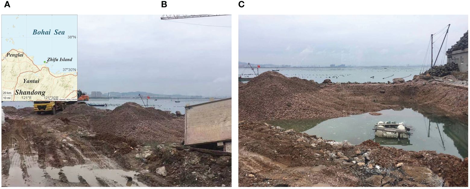
Figure 1 Accumulated scallop shells on Zhifu Island beach, Yantai city, Shandong province. (A) The green point is the area where scallop shells accumulate. (B, C) Show the specific accumulated scenario of scallop shells.
The diffusion and transportation of pollutants such as oil (Li et al., 2019b; Aslan and Otay, 2021; Cervantes-Hernández et al., 2024), microplastics (Sterl et al., 2020; Frishfelds et al., 2022), and heavy metals (Zhang et al., 2023) in the ocean are hot topics among many scholars, while little attention has been paid to the fate of scallop shells discarded in the sea. Therefore, the origins of the accumulated shells on nearshore coasts are mostly unknown, making it difficult for relevant departments to trace them, and consequently, greatly reducing the efficiency of shell resource utilization. The scallop shells transport model established in this study is coupled with a two-dimensional tidal model using the adjoint method and a Lagrangian particle tracking model to simulate the transport of scallop shells, improve shell statistics systems, and enhance the level of shell resource utilization in China. Currently, many researchers adopt two-dimensional hydrodynamic models to simulate tides and tidal currents in China’s marginal seas (Choi et al., 2014; Kuang et al., 2021; Wang et al., 2022a), with improved performance after adjoint assimilation (Jiao et al., 2023). The two-dimensional tidal model with the adjoint assimilation method can improve the accuracy of the model by assimilating data (Wang et al., 2021), separate tidal waves, simulate the current of single (Qian et al., 2021) or multiple tidal components (Wang et al., 2022b), and obtain tidal currents and residual currents. The residual current is a flow phenomenon generated when water points within a tidal wave deviate from their initial positions due to nonlinear effects after passing through one tidal cycle. Residual currents persist for a long time in nearshore areas and make significant contributions to the distribution of suspended sediment. The use of the residual current field in the research process can intuitively reflect the net transport of water (Liu et al., 2023) and serve as a basis for inferring the transport trajectories of suspended matter in seawater (Zhang et al., 2021a). To simulate the spatiotemporal profile of scallop shells in the residual current field, we can solve the partial differential equations governing advection and diffusion from a Lagrangian perspective (Capecelatro, 2018). The Lagrangian perspective solves the laws of particle displacement over time in the flow field, and can describe the particle movement process on a time scale (Das et al., 2000). Therefore, the Lagrangian model is widely used in the field of oceanography, especially in the study of particle transport in seawater, such as oil particles (Varona et al., 2024), biological larvae (Wong-Ala et al., 2022), plastic particles (Liang et al., 2021; Wisha et al., 2022), phytoplankton (Rowe et al., 2016), suspended sediment (Nakada et al., 2018), all of which can be simulated by the Lagrangian particle tracking model to study the transport process of suspended matter in the ocean.
The Bohai Sea, as a semi-enclosed marginal sea of China, is characterized mainly by shallow water features and significant tidal effects (Fang, 1986; Zhu et al., 2021). In this study, a two-dimensional tidal model with the adjoint assimilation method is established to conduct hydrodynamic research on the sea area near Yantai in the Bohai Sea. Then, a Lagrangian particle tracking model is coupled to establish a transport model for scallop shells in the Bohai Sea, simulating the transport paths of scallop shells after release under the action of dynamic factors such as residual flow, nearshore waves, and environmental factors such as temperature and salinity. The structure of this paper is as follows. Section 2 introduces the main principles and establishment of the models, and the settings of the main experimental methods. In Section 3, the experimental results are analyzed. Section 4 summarizes the results obtained, highlights the innovative points, and prospects for the future development of the model.
Under the assumptions of hydrostatic pressure, incompressible fluid, and depth-averaging, the control equations for the two-dimensional tidal model in a Cartesian coordinate system are as follows:
In Equation 1, is time, and are Cartesian coordinates (with eastward and northward directions considered positive, respectively), is the static water depth at location , is the variation in height of the free surface relative to the stationary water surface at time , and are the depth averaged velocity components of tidal currents in the and directions at time , is the Coriolis parameter, is the bottom friction coefficient, and is the horizontal eddy viscosity coefficient.
The boundary condition for the M2 tidal elevation is described as follows:
In Equation 2, and are Fourier coefficients, and is the angular frequency of the M2 constituent ().
To construct the adjoint equation, the cost function is defined as follows:
In Equation 3, is a constant (), is the model spatial domain, is the simulated value, is the observed value, and is the time step of the forward mode.
The Lagrangian function can be roughly defined as follows (Zhang and Lu, 2010):
In Equation 4, , , and represent the adjoint variables (i.e., Lagrange multipliers) corresponding to , , and , respectively. The adjoint model employs the method of discretization before differentiation as described by Gunzburger (2000). For simplicity, the indices of discrete variables have been omitted in the following equations. According to the theory of Lagrange multipliers, Equation 4 can be reformulated as follows:
Equation 5.1 represents the control equation. The adjoint equation can be expanded from Equation 5.2. Equation 5.3 can continuously optimize the model’s bottom friction coefficient and open boundary conditions during iterative computations.
Residual current is the net current velocity after a complete M2 tidal cycle. The residual current velocity on the calculation point of the model can be described as follows:
In Equation 6, is the number of times steps for the model to simulate one M2 tidal cycle (), and is the instantaneous current velocity when running for time steps.
The finite-difference formulation of the control equations and adjoint equations for the tidal flow model is similar to that described by Lu and Zhang (2006). However, due to the relatively small latitude span of the Bohai Sea (approximately 4°), we constructed the finite-difference scheme in a Cartesian coordinate system rather than a spherical coordinate system.
The model adopts the Arakawa-C grid, where the water level is located on the grid center, and the current velocity is located on the grid edges. Topex/Poseidon data, an important product of satellite remote sensing technology for observing ocean dynamics systems, are commonly used to validate the scientific integrity of constructed models (Prakash et al., 2021) and can be used for further computations. The water depth is obtained from the ETOPO 2022 dataset, with varying resolutions for different study areas. Actual Coriolis parameters are employed to study the primary M2 tide in the Bohai Sea. The main study area of this paper is the sea area adjacent to Yantai city in the Bohai Sea, where a large accumulation of scallop shells is observed (green point in Figure 2). Due to the limited availability of satellite observation data in the sea area adjacent to Yantai, we divided the Bohai Sea region into three nested areas (Figure 2A): Bohai Region I, Bohai Strait Region II, and Yantai Adjacent Region III. More specific parameters about areas are provided in Table 1.

Figure 2 The specific division and grid settings of each study area. (A) Study areas of the tidal model, with Bohai Sea Region I at a resolution of 2′×2′, Bohai Strait Region II at a resolution of 1′×1′, and the adjacent area of Yantai Region III at a resolution of 30″×30″. (B) Distribution of adjoint assimilation grid points and observation data in Region I, where black points represent model grid points, blue points represent satellite observation data, and the green point indicates the area of pollutant accumulation. (C, D) Show the distribution of adjoint assimilation grid points and observation data in Regions II and III, respectively, with black points representing model grid points, blue points representing observation data, and the green point indicating the area of pollutant accumulation.
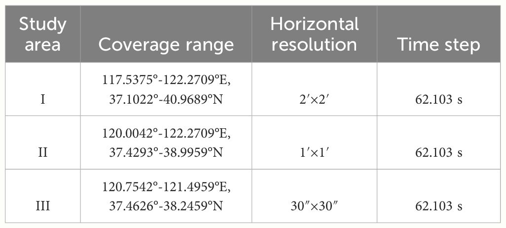
Table 1 Specific settings for each study area of the experiment.
When setting the model grid, refinement and optimization were applied to the boundary grid points based on the actual coastline and resolution. The specific division of each study area and the model grid settings are shown in Figure 2. Observation data from the Topex/Poseidon satellite altimeter was used for Region I, while data from the satellite altimeter were too sparse for Regions II and III. Therefore, in the process of nested regionalization, the simulation results from the previous level were incorporated as “observed” data into the simulation process of the next level to ensure an adequate amount of observation data for each region. For example, in Figure 2B, the black grid points in Region I correspond to the blue grid points in Region II. The simulation results from the black grid points in Region I were used as “observed” data for the blue grid points in Region II. Similarly, the simulation results from grid points in Region II were used as “observed” data for the blue grid points in Region III. Finally, using the two-dimensional tidal model, the distribution of tidal residual currents in each region was calculated.
The simulation of pollutants based on the Lagrangian particle tracking method has been widely applied and used in studies related to green tides (Han et al., 2022), oil spills (Wang et al., 2023b), and the transportation of fish feed (Wang et al., 2023a). In this study, we employed the Lagrangian particle tracking method to simulate the transport of scallop shells. Scallop shells have a three-layer structure with air pockets between the layers, which increases their actual displaced volume and decreases their density. Additionally, the discarded shells assume an open position, which is favorable for resuspension under the influence of natural forces such as tides, waves, and turbulence. Considering all these factors, we assumed that scallop shells undergo suspended motion in near-seabed areas and transport in the form of particles within the model. Therefore, during the computation, the discarded shells suspended in near-seabed areas and subject to dynamic processes. The coordinates of particles released into the sea surface can be determined as follows:
In Equation 7, is the displacement vector of the particles in the Cartesian coordinate system, which is also a function of time , is the current velocity, is the current velocity driven by waves, is the current velocity driven by wind, is the diffusion velocity of the particles induced by turbulence. The sum of the first three terms on the right side represents the drift velocity of the particles.
Our study focuses on the transport of scallop shells, a process that typically occurs near the seabed, rather than at the surface. Since wind stress directly affects surface waters, the influence of wind-induced currents is most significant in the upper layers of the water column, the effect of wind stress on the particles can be neglected. In this case, the drift velocity of the particles is mainly composed of the current velocity vector and the Stokes wave velocity vector. The velocity components in each direction can be expressed as (Zhang and Ozer, 1992):
In Equation 8, and are the horizontal velocity components of the current, with specific data provided by the residual current field output from the two-dimensional tidal model, and are the Stokes wave-induced velocity, which affects the movement trajectory of particles, causing them to tend more towards the shore in the motion simulation, aligning better with real-world conditions, is the vertical velocity of the particles.
The diffusion caused by turbulence exhibits randomness, and the diffusion velocity is calculated as follows:
In Equation 9, , , and are mutually independent and uniformly distributed random numbers in the interval [-1, 1], is the time step, is the horizontal diffusion coefficient, and is the vertical diffusion coefficient.
The horizontal diffusion coefficient is approximated using an exponential function of time (Equation 10) proposed by Pan et al. (2020):
The vertical diffusion coefficient is calculated based on the relationship proposed by Boufadel et al. (2020):
In Equation 11, = 0.4 is the von Kármán constant, is the water friction velocity, MLD is the mixed layer depth, representing the maximum depth of the boundary layer formed by the interaction between air and sea, defined here as the depth where the temperature is 0.2 °C lower than the sea surface temperature (Cao et al., 2021), and is the roughness length of the surface under regular wave action. When (at the sea surface), . The introduction of the non-zero value allows substances at the sea surface to diffuse downwards into the water column through turbulent diffusion. is calculated using the following relationship (Bandara et al., 2011):
In Equation 12, is the significant wave height, is the wind speed at 10 meters above sea level, is the phase velocity of the wave, which depends on the wave period.
The water friction velocity is calculated according to the following relationship in Equation 11 (Craig and Banner, 1994; Bandara et al., 2011):
In Equation 13, and are the air and water densities, and are the flow velocities at the sea surface and the seabed respectively, = 1.13 × 10⁻³ is the surface drag coefficient, and is the bottom drag coefficient, which can be calculated from (Li et al., 2018):
In Equation 14, zab represents the height of the water column above the seabed, and z0 represents the thickness of the mixed layer.
The calculation domain of the Lagrangian particle tracking model matches that of Region III, the sea area adjacent to Yantai, Bohai Sea, in the tidal model. The grid resolution of the model is 30’’×30’’, with a temporal resolution of 1 day. The total grid number is 95×90, and the model is divided into 10 layers vertically. Depth data is sourced from the ETOPO 2022 dataset, while the current field data is obtained from the adjoint assimilation model of the two-dimensional tidal flow simulation in Region III. Wind speed data is calculated from NCEP dataset, and the nearshore wave data is generated by the SWAN model, which is validated by Jiang et al. (2022).
In this study, based on the Lagrangian particle tracking method, two experimental schemes are employed to simulate the transport pathways of shells. Scheme one involves continuously releasing 100,000 Lagrangian particles at the center of the aquaculture area (121.165229°E, 37.692156°N) for 240 days to simulate the movement of pollutants. The specific parameters of the model are listed in Table 2. Scheme two applies simultaneously and randomly releasing 100,000 Lagrangian particles within the aquaculture area (121.165229 ± 0.01°E, 37.692156 ± 0.01°N) to simulate the movement of pollutants. The specific parameters of the model are listed in Table 3.
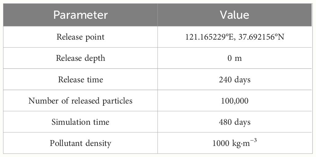
Table 2 Parameters for single-point release experiment.
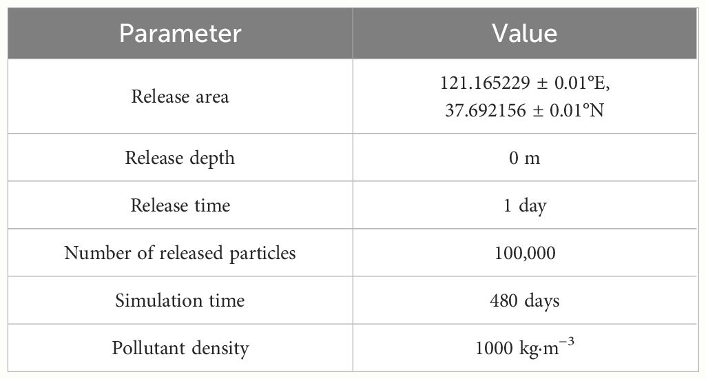
Table 3 Parameters for regional release experiment model.
The tidal residual current distribution in each region is illustrated in Figures 3–5. Due to the large coverage ranges of Regions I and II, it is challenging to depict the residual current distribution near the pollutant accumulation areas effectively. Hence, we magnify the tidal residual flow distribution near the pollutant accumulation areas in Regions I and II (Figures 3, 4).
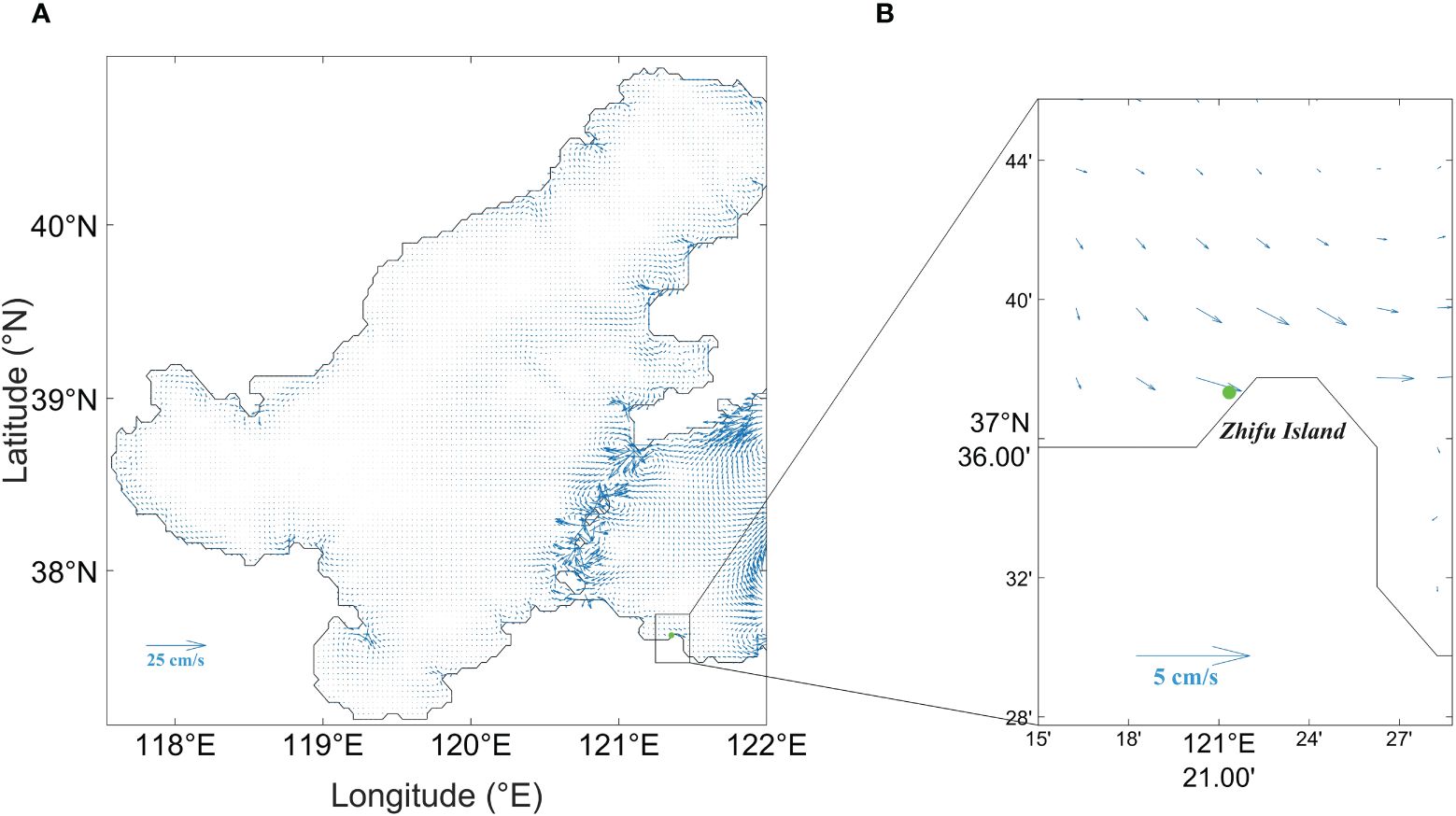
Figure 3 Tidal residual current distribution in Region I (A) (scale of 25 cm/s) and near the pollutant accumulation area (B) (scale of 5 cm/s). The green point is the pollutant accumulation point at 121.353758°E, 37.626160°N.
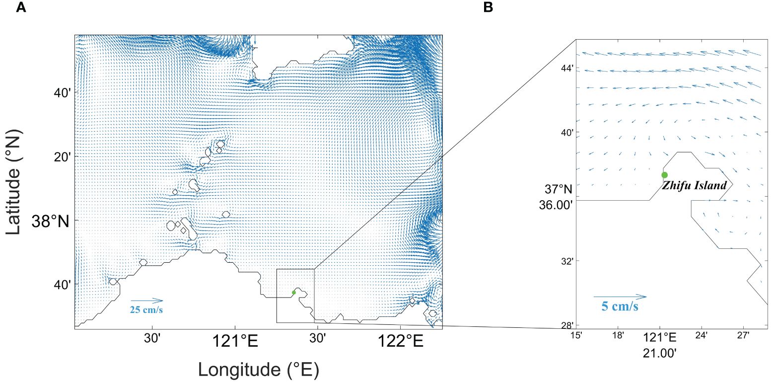
Figure 4 Tidal residual current distribution in Region II (A) (scale of 25 cm/s) and near the pollutant accumulation area (B) (scale of 5 cm/s). The green point is the pollutant accumulation point at 121.353758°E, 37.626160°N.
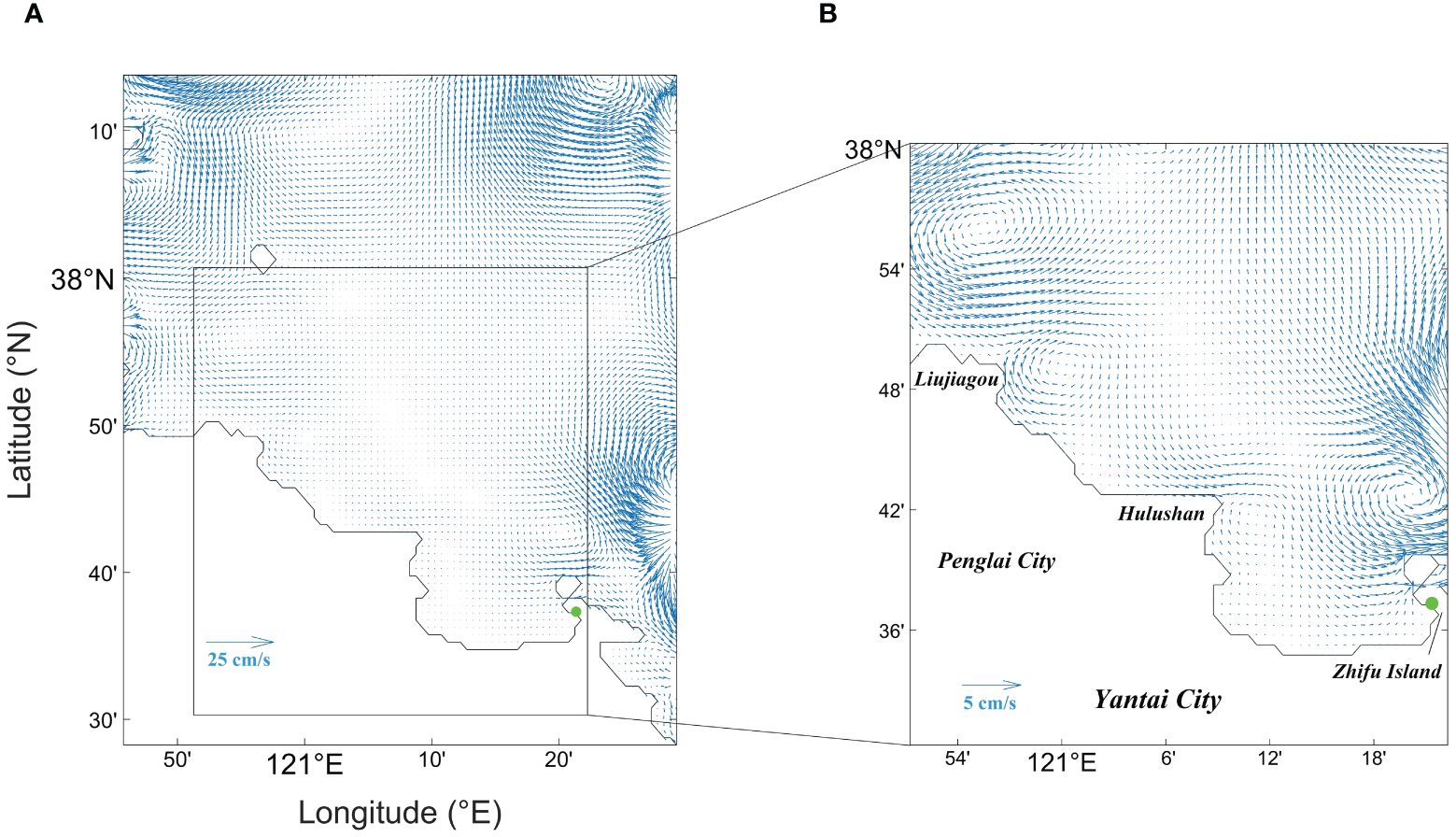
Figure 5 Tidal residual current distribution in Region III (A) (scale of 25 cm/s) and near the pollutant accumulation area (B) (scale of 5 cm/s). The green point is the pollutant accumulation point at 121.353758°E, 37.626160°N.
The residual current field (Figures 3B, 4B) can, to a certain extent, characterize the net transport process of water masses near the pollutant accumulation area, it can be observed that the water mass near the pollutant accumulation point mainly originates from the northwest and northeast currents. The northeast current is blocked by Zhifu Island. If pollutants were to be transported along the northeast current, they would accumulate north of Zhifu Island instead of the southwest, suggesting a higher possibility of pollutant movement along the northwest current. Examination of the actual situation in the northwest direction reveals shellfish aquaculture farms and processing plants near Penglai Liujiagou and Hulushan (Figure 5B), further increasing the possibility of waste shells accumulation originating from the northwest direction. Therefore, we reduce the coverage area to Region III and increase the grid resolution to 30’’. Region III focuses on the western sea area near the pollutant accumulation point, including the two suspected pollution sources. The simulation result of Region II is used as observed data for Region III simulation, yielding the residual current distribution shown in Figure 5A.
By magnifying the western sea area near the pollutant accumulation point (Figure 5B), clockwise residual currents are observed near Liujiagou, which may carry pollutants away from the coast. Subsequently, these pollutants may move southeastward along with the residual current, possibly passing near Hulushan. Likewise, clockwise residual currents near Hulushan could further propel pollutants eastward, then southward, these pollutants could eventually aggregate near the pollutant accumulation point, influenced by counterclockwise residual currents and nearshore wave effects. These pathways are speculative based on the residual current field. Next, we will use the Lagrangian particle tracking method to simulate the transport pathways of pollutants to validate our speculations.
In the Lagrangian particle tracking model, pollutants are considered particles, and simulations are conducted to study the pollutant accumulation area (Figure 5A), in the sea area adjacent to Yantai, in the Bohai Sea. Among the two suspected pollution sources near Penglai Liujiagou and Hulushan, we selected the sea area adjacent to Hulushan (121.165229°E, 37.692156°N) as the pollutant release area based on the proximity principle, residual current field, and field inspections. The model applies onshore waves in the nearshore sea areas to facilitate the shoreline movement of pollutants. To further observe the transport pathways of pollutants, two sets of Lagrangian particle tracking experiments are designed in this study to validate the possibility of pollutants aggregating near Zhifu Island (121.353758°E, 37.626160°N) originating from the sea area adjacent to Hulushan. The first set involves a single-point release experiment to observe the trajectory of pollutants released from the sea area adjacent area of Hulushan. The second set comprises a regional release experiment where pollutants are randomly released within the domain of 121.165229 ± 0.01°E, 37.692156 ± 0.01°N, simulating the movement of pollutants. Since pollutants are not released solely at one point in actual scenarios but within a certain range, the second set of experiments better reflects reality.
In this experiment, 100,000 pollutant particles were continuously released for 240 days near Hulushan (red diamond point in Figure 6), simulating the transport trajectory of pollutants. The specific parameters of the model are listed in Table 2. The experiment comprehensively considers the effects of residual current, turbulence, and nearshore waves. The transport trajectories of pollutants at different times under the influence of environmental dynamics are shown in Figure 6.
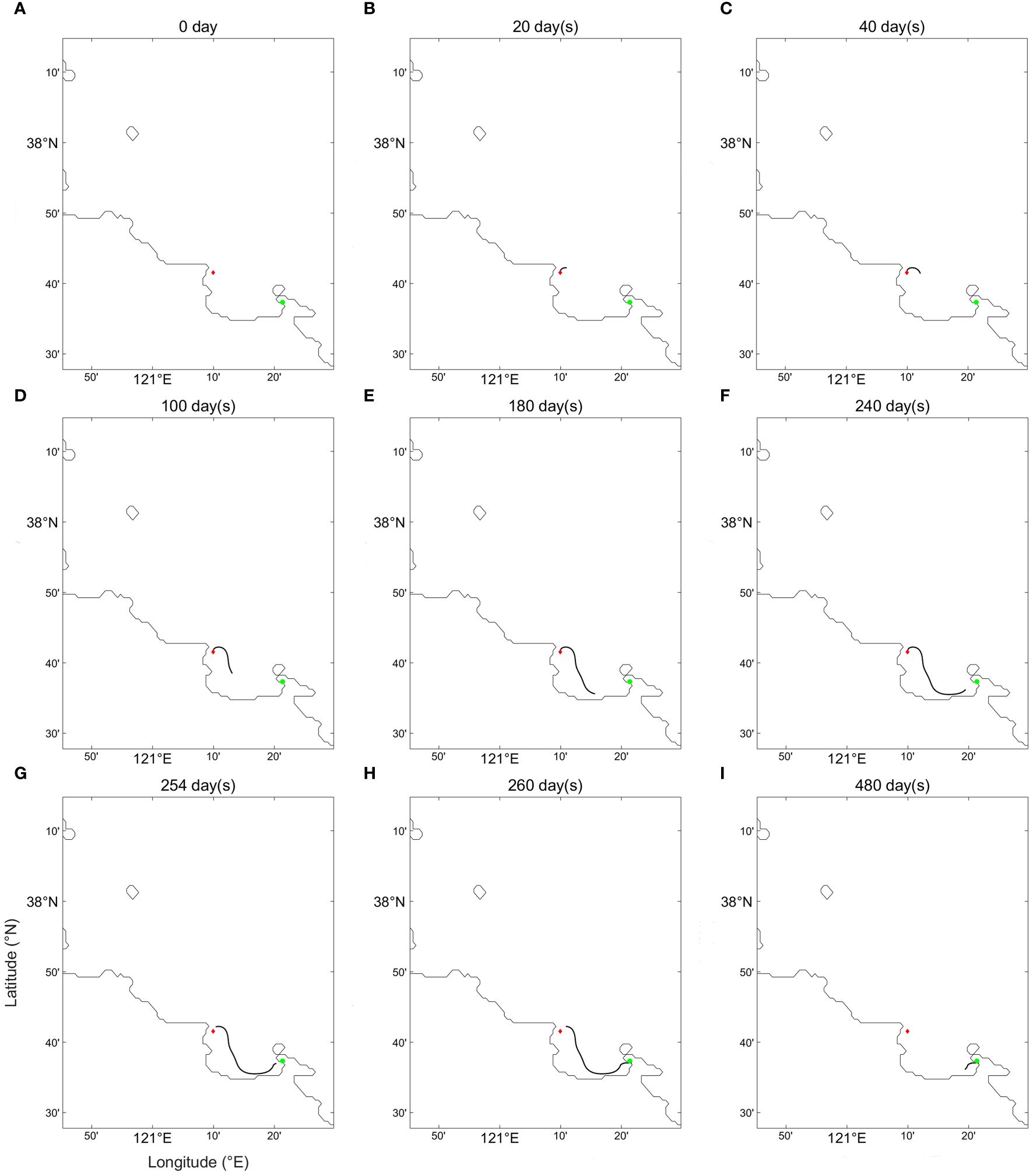
Figure 6 Transport trajectories of pollutants in the single-point release experiment at different time points: (A) 0 day, (B) 20 days, (C) 40 days, (D) 100 days, (E) 180 days, (F) 240 days, (G) 254 days, (H) 260 days, (I) 480 days.
In the simulation of the single-point release experiment, under the drive of environmental dynamics, pollutants move northeastward from the red point within 20 days after release (Figure 6B). After 40 days, pollutants begin to move southeastward (Figure 6C), exhibiting a clockwise trajectory, largely influenced by the clockwise residual current in the area. Over the next 100 days, pollutants continue to move southeastward until day 180 (Figure 6E), when their direction shifts slightly. By day 240 (Figure 6F), pollutants have started moving eastward, slightly northward, and gradually approaching the coast. On day 254 (Figure 6G), some pollutants are closer to the coast, with nearshore waves dominating environmental dynamics, pushing pollutants toward the shore. By day 260 (Figure 6H), some have reached the shore, near the pollutant accumulation point (green point in Figure 6). By day 240, all pollutant particles have entered the ocean. Once pollutants reach the shore, their movement stops as the model sets their velocity to zero. Subsequently, 93.88% of pollutants have reached the accumulation area by day 480. The results of the experiment indicate that pollutants released from a single point near Hulushan can reach the actual pollutant accumulation area under the influence of residual current, turbulence, and nearshore waves. This also suggests a high possibility that pollutants, in reality, may be released from the Hulushan.
In this experiment, pollutants were simultaneously and randomly released within the domain of 121.165229 ± 0.01°E, 37.692156 ± 0.01°N (the black square centered around a red diamond point in Figure 7), simulating the diffusion and transport pathways of pollutants in the study area over different time periods (Figure 7). The specific parameters of the model are listed in Table 3.
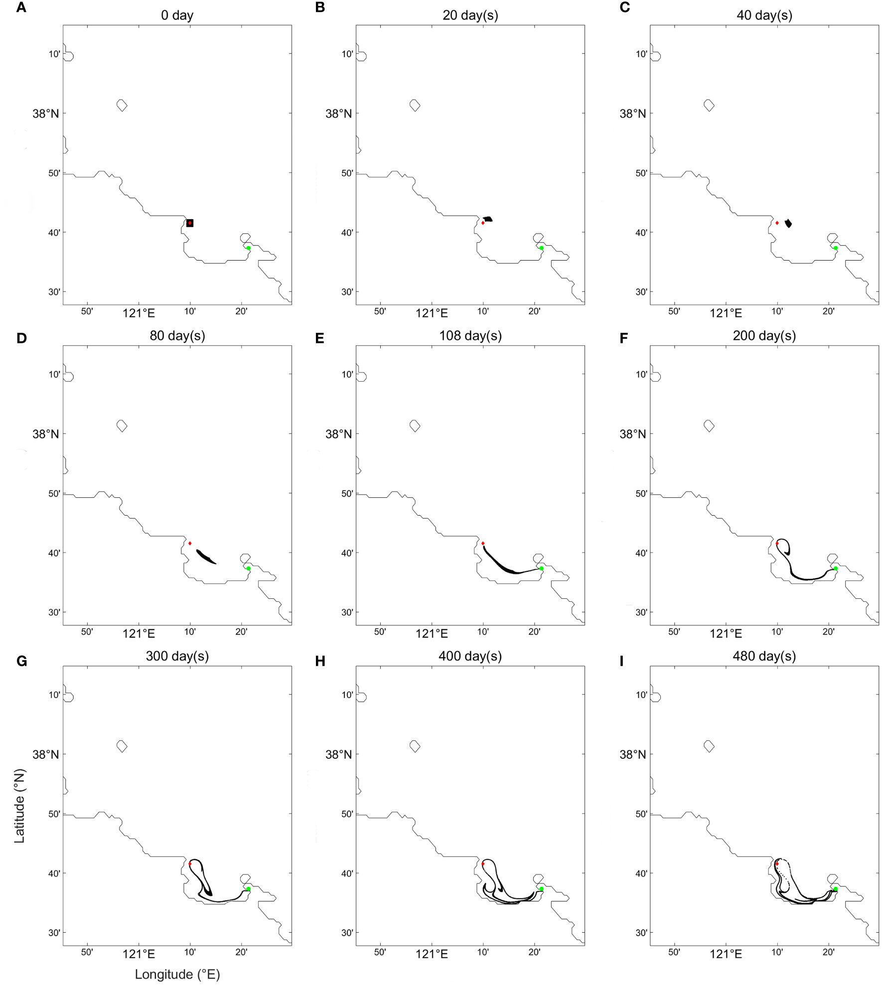
Figure 7 Transport trajectories of pollutants in the regional release experiment at different time points: (A) 0 day, (B) 20 days, (C) 40 days, (D) 80 days, (E) 108 days, (F) 200 days, (G) 300 days, (H) 400 days, (I) 480 days.
In this experiment, 100,000 pollutant particles are released (Figure 7A) in one day. These pollutants then enter the seawater, where they are suspended and gradually disperse under the influence of a clockwise residual current. Initially, owing to release together, pollutants collectively move clockwise in the sea near the release area within 40 days (Figures 7B, C). However, at day 80 (Figure 7D), due to a smaller residual current in the southeast of the release area and varying current velocities at different positions, the pollutants experience different environmental dynamics during this period. Consequently, the pollutant cluster gradually stretches out, and experiences more complex environmental dynamics. Under the influence of significant counterclockwise residual current and turbulence near the pollutant accumulation area, part of the pollutants spread eastward and eventually ashore on day 108 (Figure 7E) driven by the nearshore waves. Meanwhile, other pollutants, affected by the clockwise residual current near the release area, circulated back towards the initial release area, leaving a clockwise trajectory (Figure 7F). After 300 days (Figure 7G), pollutants are separately transported southeastward and northwestward due to residual current and turbulence. By day 400 (Figure 7H), a significant portion of the pollutants had been transported close to the accumulation area, while others began moving northwestward, influenced by the clockwise currents near the release site. By day 480 (Figure 7I), at the end of the regional release experiment, 82.57% of pollutants have reached the shore, the remaining pollutants are either stranded on other coasts or still undergone suspension in the Bohai Sea. Interestingly, the pollutants in the regional release experiment reached the accumulation area faster than in the single-point release experiment. This difference can be attributed to the fact in the latter, the residual current direction in the single-point experiment is not directly toward the accumulation point, whereas some release points in the regional release experiment have residual current directions toward the accumulation area. Overall, the results of the regional release experiment further demonstrate that pollutants released near Penglai Hulushan can be transported to the accumulation area under the influence of residual current, turbulence, and nearshore waves, consistent with real scenarios.
These two sets of experiments, designed based on known tidal residual current and nearshore wave conditions in the study area, use the Lagrangian particle tracking model to determine the specific transport pathways and dispersion ranges of suspended pollutants. Scientifically validated speculations suggest that pollutants accumulating along the Yantai coast are likely released from or pass through the vicinity of Penglai Hulushan.
This study employed a method coupling a Lagrangian particle tracking model with a two-dimensional tidal model to simulate the transport and movement of discarded scallop shells in the Bohai Sea. Given that the M2 tidal constituent dominates in the Bohai Sea, the M2 tidal residual current field was selected as the input flow field for the Lagrangian particle tracking model. Through hierarchical nested simulations in the Bohai Sea region, high-resolution M2 tidal residual current distributions near the accumulation area of scallop shells were obtained. The simulation results indicated the presence of a clockwise residual current near Hulushan in the scallop farming area and a counterclockwise residual current near Zhifu Island. Based on this, we inferred the approximate release area and likely transport direction of scallop shells. Considering the uncertainty of the release location of the shells, two sets of particle tracking experiments were designed. The experiments revealed that after entering the sea, shells initially moved northeastward under the influence of a rotating residual current, then southeastward, followed by a northeastern shift, and finally approached the coast under the influence of nearshore waves. From the moment the scallop shells were released into the sea to their arrival on the coast of Zhifu Island, it took at least 108 days. Moreover, shells were continually dispersed during their movement. By the end of the regional release experiment, scallop shells had not only accumulated on the coast of Zhifu Island, but also remained on other coasts of Yantai. The study found that most of the shells accumulated on the coast of Yantai Zhifu Island originated from or passed by Hulushan after being discarded.
However, the coupled model used in this study still has some limitations. The model ignored the shape and size of the shells themselves, treating them as homogeneous Lagrangian particles. Additionally, we assumed that the shells remained suspended in seawater and neglected the possibility of sinking due to factors other than dynamic forces, such as attachment of other organisms increasing density and causing sinking. Furthermore, it’s important to notice that the dynamic factors considered in this study only included M2 tidal residual current, turbulence, and nearshore waves, but M2 tidal residual current does not represent all tidal dynamics in the area, and the influence of ocean current in the region was not considered. Lastly, this study is only an idealized experiment and has not considered seasonal variations, such as wind, temperature and duration of scallop shells released. In future research, we plan to incorporate the residual currents of the four major tidal constituents (M2, S2, K1, O1) as well as the effect of the Bohai Sea current to improve model accuracy. In addition, we will also conduct practical experiments, setting the release time of the scallop shells based on the results of these experiments and the scallop market season, and actually considering the effects of tidal currents, wind, turbulence, and coastal waves on the transport of the scallop shells. Field visits to scallop farming bases near Penglai Hulushan will be conducted to validate the model’s conclusions and enhance its reliability. Overall, this study provides new insights into the mechanisms of discarded scallop shell pollutants transport in the Bohai Sea region, contributing to a better understanding of environmental pollution issues and marine ecological impacts in the area.
The original contributions presented in the study are included in the article/supplementary material. Further inquiries can be directed to the corresponding authors.
LC: Conceptualization, Data curation, Formal analysis, Investigation, Methodology, Software, Validation, Visualization, Writing – original draft, Writing – review & editing. YZ: Conceptualization, Methodology, Software, Writing – review & editing. YL: Conceptualization, Funding acquisition, Supervision, Writing – review & editing. RC: Conceptualization, Methodology, Software, Supervision, Writing – review & editing. XL: Conceptualization, Formal analysis, Methodology, Project administration, Resources, Supervision, Writing – review & editing.
The author(s) declare financial support was received for the research, authorship, and/or publication of this article. This work is supported by the Key R&D Program of Shandong Province (S & T Demonstration Project) (No. 2021SFGC0701) and the National Natural Science Foundation of China (Grant No. 42076011 and Grant No. U2006210).
Special thanks to Rushui Xiao, Nan Wang, and Shengyi Jiao for participating in the discussion on the study method and manuscript with useful suggestions.
The authors declare that the research was conducted in the absence of any commercial or financial relationships that could be construed as a potential conflict of interest.
All claims expressed in this article are solely those of the authors and do not necessarily represent those of their affiliated organizations, or those of the publisher, the editors and the reviewers. Any product that may be evaluated in this article, or claim that may be made by its manufacturer, is not guaranteed or endorsed by the publisher.
Aslan M., Otay E. N. (2021). Exchange of water and contaminants between the Strait of Istanbul and the Golden Horn. Ocean Eng. 230, 108984. doi: 10.1016/j.oceaneng.2021.108984
Bandara U. C., Yapa P. D., Xie H. (2011). Fate and transport of oil in sediment laden marine waters. J. Hydro-environment Res. 5, 145–156. doi: 10.1016/j.jher.2011.03.002
Boufadel M., Liu R., Zhao L., Lu Y., Özgökmen T., Nedwed T., et al. (2020). Transport of oil droplets in the upper ocean: impact of the eddy diffusivity. JGR Oceans 125, e2019JC015727. doi: 10.1029/2019JC015727
Cao R., Chen H., Rong Z., Lv X. (2021). Impact of ocean waves on transport of underwater spilled oil in the Bohai Sea. Mar. pollut. Bull. 171, 112702. doi: 10.1016/j.marpolbul.2021.112702
Capecelatro J. (2018). A purely Lagrangian method for simulating the shallow water equations on a sphere using smooth particle hydrodynamics. J. Comput. Phys. 356, 174–191. doi: 10.1016/j.jcp.2017.12.002
Cervantes-Hernández P., Celis-Hernández O., Ahumada-Sempoal M. A., Reyes-Hernández C. A., Gómez-Ponce M. A. (2024). Combined use of SAR images and numerical simulations to identify the source and trajectories of oil spills in coastal environments. Mar. pollut. Bull. 199, 115981. doi: 10.1016/j.marpolbul.2023.115981
Choi B., Hwang C., Lee S. (2014). Meteotsunami-tide interactions and high-frequency sea level oscillations in the eastern Yellow Sea. JGR Oceans 119, 6725–6742. doi: 10.1002/2013JC009788
Craig P. D., Banner M. L. (1994). Modeling wave-enhanced turbulence in the ocean surface layer. J. Phys. Oceanography 24, 2546–2559. doi: 10.1175/1520-0485(1994)024<2546:MWETIT>2.0.CO;2
Das P., Marchesiello P., Middleton J. H. (2000). Numerical modelling of tide-induced residual circulation in Sydney Harbour. Mar. Freshw. Res. 51, 97. doi: 10.1071/MF97177
Fang G. (1986). Tide and tidal current charts for the marginal seas adjacent to China. Chin. J. Ocean. Limnol. 4, 1–16. doi: 10.1007/BF02850393
Frishfelds V., Murawski J., She J. (2022). Transport of microplastics from the daugava estuary to the open sea. Front. Mar. Sci. 9. doi: 10.3389/fmars.2022.886775
Gunzburger M. (2000). Adjoint equation-based methods for control problems in incompressible, viscous flows. Flow Turbulence Combustion. 65, 249–272. doi: 10.1023/A:1011455900396
Han X., Kuang C., Li Y., Song W., Qin R., Wang D. (2022). Numerical modeling of a green tide migration process with multiple artificial structures in the Western Bohai Sea, China. Appl. Sci. 12, 3017. doi: 10.3390/app12063017
Jiang Y., Rong Z., Li P., Qin T., Yu X., Chi Y., et al. (2022). Modeling waves over the Changjiang River Estuary using a high-resolution unstructured SWAN model. Ocean Model. 173, 102007. doi: 10.1016/j.ocemod.2022.102007
Jiao S., Zhang Y., Pan H., Lv X. (2023). Improved estimation of the open boundary conditions in tidal models using trigonometric polynomials fitting scheme. Remote Sens. 15, 480. doi: 10.3390/rs15020480
Kuang C., Han X., Zhang J., Zou Q., Dong B. (2021). Morphodynamic evolution of a nourished beach with artificial sandbars: field observations and numerical modeling. JMSE 9, 245. doi: 10.3390/jmse9030245
Li C. (2017). “A new way of handling shells,” in People’s Daily Oversea, vol. 4. (China: Chenyang Li), vol. 4. Available at: http://paper.people.com.cn/rmrbhwb/html/2017-07/04/content_1787897.htm.
Li Y., Chen H., Lv X. (2018). Impact of error in ocean dynamical background, on the transport of underwater spilled oil. Ocean Model. 132, 30–45. doi: 10.1016/j.ocemod.2018.10.003
Li Y., Yan L., Yu D., Tian Y., Liu J. (2019a). Comparison of air exposure stress resistances of post-harvested yesso scallop with different sizes. Fisheries Sci. 38, 443–450. doi: 10.16378/j.cnki.1003-1111.2019.04.002
Li Y., Yu H., Wang Z., Li Y., Pan Q., Meng S., et al. (2019b). The forecasting and analysis of oil spill drift trajectory during the Sanchi collision accident, East China Sea. Ocean Eng. 187, 106231. doi: 10.1016/j.oceaneng.2019.106231
Liang J., Liu J., Benfield M., Justic D., Holstein D., Liu B., et al. (2021). Including the effects of subsurface currents on buoyant particles in Lagrangian particle tracking models: Model development and its application to the study of riverborne plastics over the Louisiana/Texas shelf. Ocean Model. 167, 101879. doi: 10.1016/j.ocemod.2021.101879
Liu L., Yuan D., Li X., Mao Y. (2023). Influence of reclamation on the water exchange in Bohai Bay using trajectory clustering. Stoch Environ. Res. Risk Assess. 37, 3571–3583. doi: 10.1007/s00477-023-02463-8
Lu X., Zhang J. (2006). Numerical study on spatially varying bottom friction coefficient of a 2D tidal model with adjoint method. Continental Shelf Res. 26, 1905–1923. doi: 10.1016/j.csr.2006.06.007
Nakada S., Hayashi M., Koshimura S. (2018). Transportation of sediment and heavy metals resuspended by a giant tsunami based on coupled three-dimensional tsunami, ocean, and particle-tracking simulations. J. Wat. Envir. Tech 16, 161–174. doi: 10.2965/jwet.17-028
Pan Q., Yu H., Daling P. S., Zhang Y., Reed M., Wang Z., et al. (2020). Fate and behavior of Sanchi oil spill transported by the Kuroshio during January–February 2018. Mar. pollut. Bull. 152, 110917. doi: 10.1016/j.marpolbul.2020.110917
Prakash N., Ashly K. U., Seelam J. K., Bhaskaran H., Yadhunath E. M., Lavanya H., et al. (2021). Investigation of near-shore processes along North Goa beaches: A study based on field observations and numerical modelling. J. Earth Syst. Sci. 130, 242. doi: 10.1007/s12040-021-01755-3
Qian S., Wang D., Zhang J., Li C. (2021). Adjoint estimation and interpretation of spatially varying bottom friction coefficients of the M 2 tide for a tidal model in the Bohai, Yellow and East China Seas with multi-mission satellite observations. Ocean Model. 161, 101783. doi: 10.1016/j.ocemod.2021.101783
Rowe M. D., Anderson E. J., Wynne T. T., Stumpf R. P., Fanslow D. L., Kijanka K., et al. (2016). Vertical distribution of buoyant Microcystis blooms in a Lagrangian particle tracking model for short-term forecasts in Lake Erie. JGR Oceans 121, 5296–5314. doi: 10.1002/2016JC011720
Shi B., Gong P., Guan C., Zhao R., Li J. (2019). Influence of different replacement rates of argopecten irradias aggregate on physical properties of artificial reefs and carbon sequestration. Prog. Fishery Sci. 40, 1–8. doi: 10.19663/j.issn2095-9869.20181222002
Sterl M. F., Delandmeter P., Van Sebille E. (2020). Influence of barotropic tidal currents on transport and accumulation of floating microplastics in the global open ocean. JGR Oceans 125, e2019JC015583. doi: 10.1029/2019JC015583
Varona H. L., Noriega C., Calzada A. E., Medeiros C., Lobaina A., Rodriguez A., et al. (2024). Effects of meteo-oceanographic conditions on the weathering processes of oil spills in northeastern Brazil. Mar. pollut. Bull. 198, 115828. doi: 10.1016/j.marpolbul.2023.115828
Wang D., Wu F. (Eds.) (2021). “Part II. Production,” in CHINA FISHERY STATISTICAL YEARBOOK (China: China Agriculture Press), 15 + 17–46. doi: 10.43455/y.cnki.yzytn.2022.000001
Wang D., Zhang J., Wang Y. P. (2021). Estimation of bottom friction coefficient in multi-constituent tidal models using the adjoint method: temporal variations and spatial distributions. JGR Oceans 126, e2020JC016949. doi: 10.1029/2020JC016949
Wang J., Kuang C., Ou L., Zhang Q., Qin R., Fan J., et al. (2022a). A simple model for a fast forewarning system of brown tide in the coastal waters of Qinhuangdao in the Bohai Sea, China. Appl. Sci. 12, 6477. doi: 10.3390/app12136477
Wang N., Cao R., Lv X., Shi H. (2023a). Research on the transport of typical pollutants in the yellow sea with flow and wind fields. JMSE 11, 1710. doi: 10.3390/jmse11091710
Wang Q., Lü Y., He L., Huang X., Feng J. (2023b). Simulating oil droplet underwater dispersal from a condensate field spill in the South China Sea. Ocean Eng. 284, 115090. doi: 10.1016/j.oceaneng.2023.115090
Wang Q., Zhang Y., Wang Y., Xu M., Lv X. (2022b). Fitting cotidal charts of eight major tidal components in the bohai sea, yellow sea based on chebyshev polynomial method. JMSE 10, 1219. doi: 10.3390/jmse10091219
Wisha U. J., Gemilang W. A., Wijaya Y. J., Purwanto A. D. (2022). Model-based estimation of plastic debris accumulation in Banten Bay, Indonesia, using particle tracking - Flow model hydrodynamics approach. Ocean Coast. Manage. 217, 106009. doi: 10.1016/j.ocecoaman.2021.106009
Wong-Ala J. A. T. K., Ciannelli L., Durski S. M., Spitz Y. (2022). Particle trajectories in an eastern boundary current using a regional ocean model at two horizontal resolutions. J. Mar. Syst. 233, 103757. doi: 10.1016/j.jmarsys.2022.103757
Yan C., Gu Z., Zhang H., Wang Y., Shi Y., Zhan X., et al. (2012). Correlation and path analysis of major quantitative traits of Chlamys nobilis in Sanya. South China Fisheries Sci. 8, 34–38. doi: 10.3969/j.issn.2095-0780.2012.03.005
Zhang B., Ozer J. (1992). SURF -A simulation model for the behaviour of oil slicks at sea. Available online at: https://api.semanticscholar.org/CorpusID:221993828.
Zhang B., Pu A., Jia P., Xu C., Wang Q., Tang W. (2021a). Numerical simulation on the diffusion of alien phytoplankton in Bohai Bay. Front. Ecol. Evol. 9. doi: 10.3389/fevo.2021.719844
Zhang J., Lu X. (2010). Inversion of three-dimensional tidal currents in marginal seas by assimilating satellite altimetry. Comput. Methods Appl. Mechanics Eng. 199, 3125–3136. doi: 10.1016/j.cma.2010.06.014
Zhang L., Wu Y., Ni Z., Li J., Ren Y., Lin J., et al. (2023). Saltwater intrusion regulates the distribution and partitioning of heavy metals in water in a dynamic estuary, South China. Mar. Environ. Res. 186, 105943. doi: 10.1016/j.marenvres.2023.105943
Zhang R., Gao B., Guo L., Wu J., Peng Y., Chen Q. (2021b). Advances in research on the use of shellfish wastes to passivate heavy metals in soil. J. Agric. Resour. Environ. 38, 787–796. doi: 10.13254/j.jare.2020.0504
Keywords: adjoint assimilation, Lagrangian particle tracking, Bohai Sea, tidal residual current, pollutant transport
Citation: Chen L, Zhang Y, Liu Y, Cao R and Lv X (2024) Research on scallop shells transport of the Yantai coastal region in the Bohai Sea. Front. Mar. Sci. 11:1425697. doi: 10.3389/fmars.2024.1425697
Received: 30 April 2024; Accepted: 14 June 2024;
Published: 05 July 2024.
Edited by:
Henrik Kalisch, University of Bergen, NorwayReviewed by:
José Pinho, University of Minho, PortugalCopyright © 2024 Chen, Zhang, Liu, Cao and Lv. This is an open-access article distributed under the terms of the Creative Commons Attribution License (CC BY). The use, distribution or reproduction in other forums is permitted, provided the original author(s) and the copyright owner(s) are credited and that the original publication in this journal is cited, in accordance with accepted academic practice. No use, distribution or reproduction is permitted which does not comply with these terms.
*Correspondence: Yongzhi Liu, eXpsaXVAZmlvLm9yZy5jbg==; Ruichen Cao, Y3JjQHN0dS5vdWMuZWR1LmNu
Disclaimer: All claims expressed in this article are solely those of the authors and do not necessarily represent those of their affiliated organizations, or those of the publisher, the editors and the reviewers. Any product that may be evaluated in this article or claim that may be made by its manufacturer is not guaranteed or endorsed by the publisher.
Research integrity at Frontiers
Learn more about the work of our research integrity team to safeguard the quality of each article we publish.