Dynamics of phytoplankton communities in the Baltic Sea: insights from a multi-dimensional analysis of pigment and spectral data—part I, pigment dataset

This study aims to investigate the seasonal and spatial distribution of surface phytoplankton communities in the Baltic Sea, using pigment analysis and hydrological parameters. Data were collected during six oceanographic campaigns between 2005 and 2008, including high-performance liquid chromatography (HPLC) pigment characterization and hydrological measurements. The first part of this comprehensive study was focused on the HPLC phytoplankton pigment dataset in relation to hydrological conditions. The research highlighted the importance of high-quality input data for accurate taxonomic analysis. Several unsupervised machine learning approaches, such as hierarchical cluster analysis (HCA), principal component analysis (PCA), and network-based community detection analysis (NCA), were used to analyze the data and identify phytoplankton communities based on biomarker pigments. Five main phytoplankton communities were identified: diatoms, dinoflagellates, cryptophytes, green algae, and cyanobacteria. The results evidenced distinct seasonal patterns, with diatom blooms dominating in spring, cyanobacterial blooms in mid-summer, and haptophyte and dinoflagellate peaks occurring in late summer and autumn. While PCA and NCA provided consistent insights into community structure, HCA offered less clarity in distinguishing between groups. The results of the statistical analysis were then compared with those of traditional approaches such as CHEMTAX and region-specific bio-optical algorithms, providing new perspectives on the taxonomic composition of phytoplankton groups. This study provides valuable insights into phytoplankton dynamics in the Baltic Sea and the effectiveness of different analytical approaches in understanding community structure, providing metrics that can enhance current and future advancements in remote sensing, including support for hyperspectral ocean color remote sensors.

1 Introduction

Phytoplankton play a crucial role in the marine ecosystem, acting as primary producers that form the base of the aquatic food web. The phytoplankton community composition influences the marine food chain and the regional carbon cycle. Monitoring phytoplankton distribution is important not only for aquatic sciences but also due to growing societal needs. Human activities, such as overfishing, pollution, and nutrient loading, severely threaten aquatic ecosystems (Lotze et al., 2006). Environmental factors such as temperature, light availability, nutrient concentrations, and water currents significantly influence phytoplankton dynamics. The unique brackish water conditions of the Baltic Sea, with salinity levels ranging from almost fresh in the Bothnian Bay (Schmelzer et al., 2008) to more saline in the southern regions (Axe and Sahlsten, 2001), create a diverse environment that supports a wide variety of phytoplankton species. Seasonal variations lead to distinct phytoplankton blooms, particularly in spring and summer, which are crucial periods for primary productivity. Increased eutrophication has led to more frequent harmful algal blooms in coastal areas, raising public concern, as these blooms affect recreation, fisheries, and drinking water supplies.

Recent technological advancements, including satellite remote sensing and high-performance liquid chromatography (HPLC), have enhanced the monitoring and understanding of phytoplankton communities. This approach includes abundance-based, spectral-based, and ecological-based methods (Nair et al., 2008; Brewin et al., 2010; IOCCG, 2014). In recent years, there has been encouraging progress in investigating the composition of biomarker pigments and the correlation between pigments and cell size. This research has been carried out using extensive datasets of phytoplankton pigments, which have been characterized by HPLC (Vidussi et al., 2001; Uitz et al., 2006; Brewin et al., 2010; Hirata et al., 2011; Mouw et al., 2017; Sun et al., 2022). HPLC is a powerful analytical technique used to separate, identify, and quantify analytical components in a mixture. In the context of phytoplankton research, HPLC allows for the precise characterization of pigment composition in discrete natural water samples, distinguishing among a wide range of pigment molecules. The relative abundance of various phytoplankton groups can be inferred by analyzing the specific pigment composition (as detailed in Supplementary Table S1), providing insights into the presence and abundance of different phytoplankton groups and ecological dynamics of phytoplankton communities. These approaches facilitate the categorization of phytoplankton into distinct size groups and are often based on the widely used CHEMTAX tool. CHEMTAX employs matrix factorization and known pigment ratios to determine the composition of taxonomic groups and has been already used in the Baltic Sea context (Schlüter et al., 2000, 2004, 2016).

Numerous studies have investigated the taxonomic composition of phytoplankton communities in the Baltic Sea (Wasmund et al., 1998; Wasmund and Uhlig, 2003, 2008, 2011; Olli et al., 2011; HELCOM, 2018). They have traditionally relied on methods such as light microscopy and flow cytometry. However, it has become clear that relying solely on discrete in situ observations to monitor phytoplankton communities is not sufficient. This is mainly due to the lack of comprehensive and extensive spatiotemporal datasets. Tools based on biomarker pigments can help track phytoplankton distribution and composition, providing essential data for managing the health of the Baltic Sea ecosystem and addressing issues such as harmful algal blooms. While several studies have investigated the chemotaxonomic characterization of Baltic phytoplankton communities based on pigment relationships (Schlüter et al., 2000; Stoń-Egiert and Ostrowska, 2022) and the development of bio-optical algorithms (Meler et al., 2020), most of these investigations have been tailored to the Southern Baltic Sea. There remains a noticeable gap in research on the wider Baltic Sea basin.

The present study aimed to evaluate data analysis methodologies that can be applied to investigate the relationship between phytoplankton community structure and pigment composition in the whole Baltic Sea. This study was based on a complete dataset that provided adequate spatiotemporal coverage of this basin and included measurements of HPLC pigments and physical variables. The identification of phytoplankton communities through various statistical data analysis methods was applied to the HPLC pigment dataset, representative of different sub-regions of the Baltic Sea, and collected over 5 years, in conjunction with optical property measurements. The dataset was subjected to three types of statistical analysis: hierarchical cluster analysis (HCA), principal component analysis (PCA), and network-based community detection analysis (NCA). The insights gained from these analyses were then compared with those derived from traditional approaches, such as CHEMTAX (Mackey et al., 1996), and region-specific bio-optical algorithms for estimating phytoplankton functional type (PFT) and size (PSC) composition (Brewin et al., 2010; Hirata et al., 2011).

2 Materials and methods

2.1 Field dataset

The datasets were collected between 2004 and 2008 during six bio-optical oceanographic campaigns: three covering the Southern Baltic Sea, Gdansk Bay, and the Pomeranian Bay (May and September 2004 and April 2005) and three in the Northern Baltic Proper, Gulf of Finland, and the Bothnian Sea (July 2006, August 2007, and August 2008) (Figure 1). The whole Baltic Sea dataset (BA) is composed of 273 stations.

Figure 1

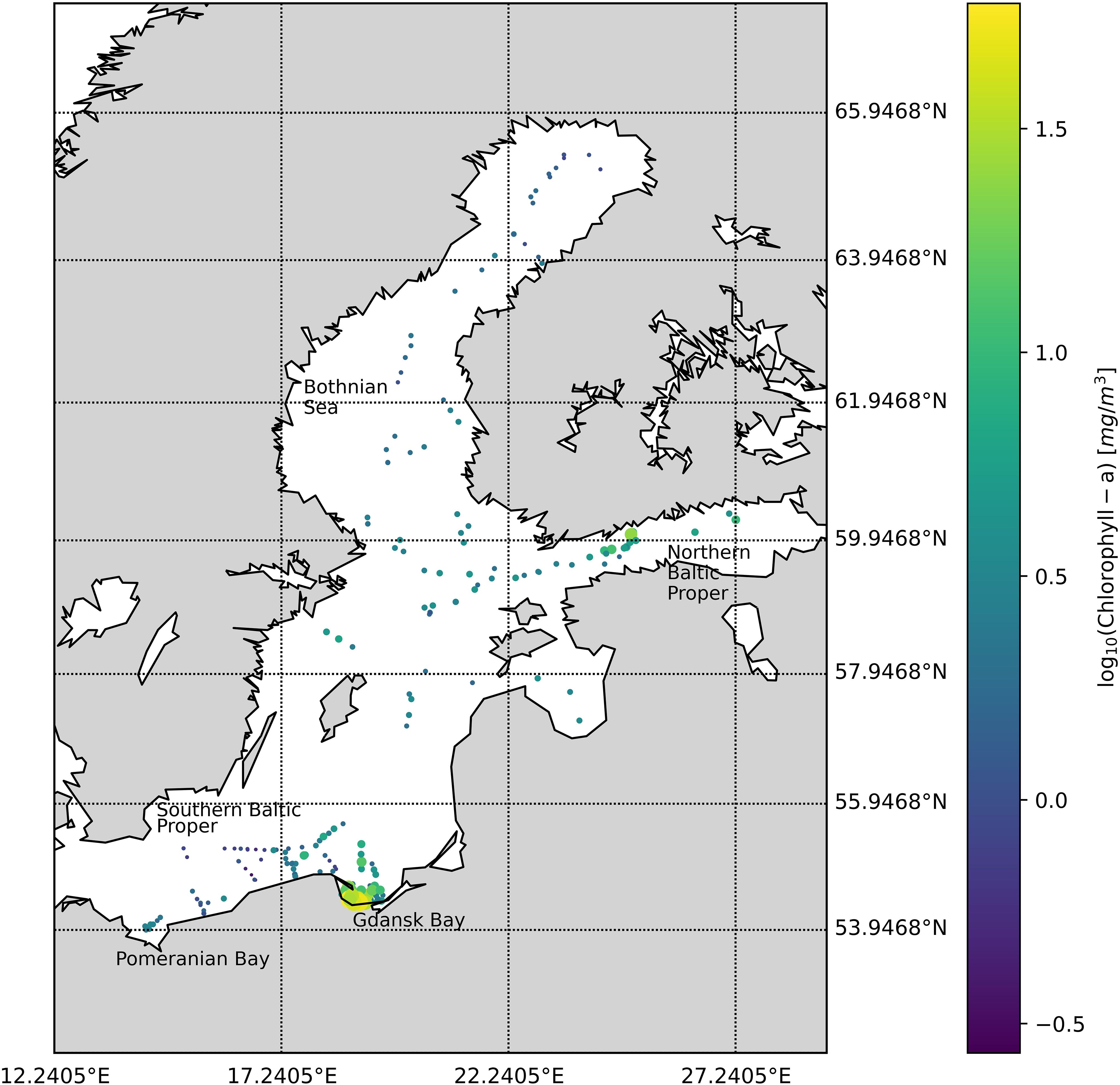
Figure 1. Spatial distribution of measuring stations in 2004–2008 shows the location and the associated TChl a (mg/m³) concentration.

Sea-surface temperature (SST) and salinity were measured using the SBE 911 Conductivity Depth Temperature (CTD) system (SeaBird, Alifax, Bellevue, Washington, USA). The water was sampled using a Niskin bottle at surface depth (1 m below the sea surface) and pre-filtered through a 150-μm mesh (Kartel, LABWARE Division, Milan, Italy). The filters (GF/F filters, Φ 25 mm, 0.7-μm pore size, Whatman, Dassel, Germany) for HPLC measurements were preconditioned under constant mild vacuum (not exceeding 0.5 bar), flash frozen in liquid nitrogen, and successively stored a −80°C.

2.2 Phytoplankton pigment dataset

HPLC samples were analyzed at the Joint Research Centre of the European Commission (JRC).

The JRC method is described in detail in Canuti (2023). The HPLC was calibrated with pigment standards (DHI Lab Products, Hørsholm, Denmark). The calibration curves and consequently the compound quantification cover a range of concentrations from a dilution close to three times the signal-to-noise ratio (SNR) concentration to the standard concentration, as described by Hooker et al. (2005). The compounds below the limit of detection (LOD) were considered unidentified. The JRC follows strict quality control measures for the analysis of phytoplankton pigments using HPLC and regularly participates in inter-laboratory exercises and inter-comparison activities to assess the uncertainties associated with marine pigments (Hooker et al., 2010; Canuti et al., 2016, 2022, Canuti, 2023).

Twenty-two pigments were quantified for all stations (Supplementary Table S1): 19′-hexanoyloxyfucoxanthin (Hex), 19′-butanoyloxyfucoxanthin (But), alloxanthin (Allo), fucoxanthin (Fuco), peridinin (Peri), diatoxanthin (Diato), diadinoxanthin (Diadino), zeaxanthin (Zea), divinyl chlorophyll a (DVChl a), monovinyl chlorophyll a (MVChl a), monovinyl chlorophyll b (MVChl b), divinyl chlorophyll d (DVChl b) chlorophyll c1 + c2 (TChl c1c2), chlorophyll c3 (TChl c3), neoxanthin (Neo), violaxanthin (Viola), prasinoxanthin (Pras), lutein (Lut), carotene (Caro), pheophorbide a (Pheo), pheophytin a (Phy), and chlorophyllide a (Chlide a).

The pigments considered for the clustering statistical analysis were 16 of those determined by HPLC, and total chlorophyll a (TChl a) is the sum of MVChl a, DVChl a, and Chlide a. Of the other pigments, Pheo, Phy, Chlide a, and DVChl a, were excluded because they were detected in concentrations lower than the LOD for more than 95% of the stations. MVChl a was not included among pigment objects of statistical analysis because it is considered a redundant accessory pigment (i.e., is a component of TChl a). Similarly, for total chlorophyll b (TChl b), the choice of considering the sum of MVChl b and DVChl b pigments (i.e., TChl b) instead of their separate contribution was due to the lack of chromatographic separation: it was not possible to discriminate the MV and DV components for all the sampling stations.

The pigment compositions and their relative proportions in phytoplankton cells are distinctive features of different classes of algae and cyanobacteria, so pigments may serve as unique taxonomic identifiers for phytoplankton (Wright et al., 1991). Certain carotenoids, which are quantitatively dominant, are considered taxonomic markers of phytoplankton. Fuco is a marker for diatoms, Zea for blue-green algae (cyanobacteria), Allo for cryptophytes, Hex for prymnesiophytes, Pras for prasinophytes, Per for dinophytes, and TChl b, Neo, and Lut for green algae (Chlorophyceae). Determining the phytoplankton community structure based on pigment compositions and concentrations has become a standard practice (Mackey et al., 1996; Rodriguez et al., 2002). However, some pigments (i.e., Fuco) are common to multiple phytoplankton groups (Supplementary Table S1), and experiments have shown that the qualitative and quantitative proportions of pigments can vary even within cells of organisms from the same class, so it is acknowledged that using a pigment as a marker for a specific group remains a simplification (Jeffrey et al., 1997, Seppala, 2009, Roy et al., 2011).

2.3 Methods in data analysis

2.3.1 Hierarchical cluster analysis

A hierarchical cluster analysis was performed on the HPLC pigment dataset using all 16 pigments described above after normalization to TChl a (i.e., using ratios of Fuco: TChla). This method uses Ward’s linkage method (the inner squared distance) based on the correlation distance (1 − R, where R is Pearson’s correlation coefficient between phytoplankton pigment ratios), as in Latasa and Bidigare (1998) and Catlett and Siegel (2018). A linkage cutoff distance of 1 was used to divide the resulting dendrogram into distinct phytoplankton community clusters. The correlation distances between samples were then used to assign each sample to one of the resulting clusters.

2.3.2 Principal component analysis

Empirical orthogonal function (EOF) analysis serves as a valuable tool for exploring potential spatial patterns of variability and their temporal evolution (Anderson et al., 2008; Barrón et al., 2014; Bracher et al., 2015; Kramer et al., 2020). In the field of statistics, this analysis is recognized as PCA. Essentially, PCA decomposes a dataset into mathematically orthogonal (independent) modes, which can be interpreted as distinctive patterns or structures within the data. We defined X as the pigment matrix, where each row (M) corresponds to a sampling station and each column (N) corresponds to the 16 variables (i.e., the 16 pigments normalized by TChl a). The standardized matrix X underwent singular value decomposition (SVD) to derive the PCA modes:

$\begin{array}{ll}\text{X}=\text{U}{\displaystyle \sum {\text{V}}^{\text{T}}},\text{\hspace{0.17em}\hspace{0.17em}\hspace{0.17em}where\hspace{0.17em}}{\text{x}}_{\text{ij}}={\displaystyle {\sum }_{k=1, N}{u}_{ik}{\sigma }_k{v}_{kj}}& (1)\end{array}$

In this equation, V is an N × N matrix containing the pigment concentration data, U is an M × N matrix containing the principal components, Σ is an N × N matrix containing the singular values along the diagonal, and k represents the index of the PCA mode (with a length of N).

The columns of X are the principal components. We refer to the columns of U as the loadings, representing the directions (or weights) in the original variable space that defines each principal component. Eigenvalues and eigenvectors are used to compute the principal components. The eigenvalues represent the amount of variance explained by each principal component, and the corresponding eigenvectors (columns of U) represent the direction of maximum variance in the original variable space. Typically, the majority of variance, or “power”, is captured by the first few modes. We focus on visualizing and summarizing the key features of these original 16 variables through the presentation of the top principal components (PCs). It is worth noting that PCA does not impose any preconceived assumptions about the underlying covariance of pigments.

2.3.3 Network-based community detection analysis

The initial step in constructing a network within the pigment’s dataset involves defining a similarity matrix between the pigment ratios, which are treated as the network’s features in this context. We adopted the absolute value of Pearson’s correlation coefficient, a common method for assessing co-expression (Allocco et al., 2004), as our evaluation metric. This approach results in the creation of a weighted, nearly fully connected graph with minimal zero values in the similarity matrix, thus limiting the identification of specific interaction clusters.

To establish a graph based on pairwise similarities, a straightforward strategy was used: we connected all pairs of nodes with non-zero similarity values and assigned edge weights corresponding to these similarity values. In our specific case, we first transformed the HPLC pigment dataset into a symmetrical adjacency matrix. Each node, or vertex, represents a sampling station, while edges connecting two nodes indicate the correlation across pigments between these stations—essentially, the relationship between any two of the 273 sampling sites. The edge weights provide insight into the strength of these connections, with Pearson’s correlation coefficients serving as the means to describe the associations between nodes, primarily based on the normalized pigment ratios to TChl a. Based on this assumption, we can describe the similarity matrix as follows:

$\begin{array}{ll}{s}_{ij}=\left|corr(x_i,x_j)\right|& (2)\end{array}$

where s_ij is the similarity matrix, corr(x_i,x_j) is Pearson’s correlation coefficient between nodes (sampling sites), and x_i and x_j are concentrations of the pigments at the different sampling sites.

However, Mason et al. (2009) provided evidence that utilizing the absolute value of the correlation may obscure biologically significant insights in unsigned networks. To quantify the strength of connections between features (i.e., pigment ratios), we employed an adjacency matrix, denoted as A = [a_ij]. This matrix A was constructed by applying a threshold to the similarity matrix S = [s_ij].

In reference to the weighted gene co-expression network analysis (WGCNA) algorithm for network construction (Zhang and Horvath, 2005), which was designed for datasets of similar dimensions, we employed the following power function to evaluate the strength of connections between nodes:

$\begin{array}{ll}{\text{a}}_{\text{ij}}={(s_{ij})}^{\beta }& (3)\end{array}$

where the power β is the soft thresholding, with the default value β = 6 for the unsigned network.

Subsequently, the analysis of the network’s community detection was performed on the adjacency matrix denoted as a_ij. This analysis was conducted using the undirected modularity method from NetworkX (Hagberg et al., 2008) in Python. To partition the community effectively, we employed Louvain’s algorithm (Blondel et al., 2008). This algorithm identifies the optimal number and type of communities that maximize the network’s modularity score.

Modularity, in this context, is a metric that falls within the range of −0.5 to 1, indicating the density of edges within communities compared to edges that extend outside of communities. It quantifies the level of connectedness within the network’s communities. A modularity score of 0.3 or higher is considered substantial, signifying strong interconnections among sites within each community and weaker connections between different groups.

The modularity output provides a community assignment for every sampling site within the matrix, reflecting the interrelatedness of the considered pigment ratios. To assess the taxonomic relevance of each community, we relied on the mean ratios of biomarker pigments within these communities: for the samples in the community, we considered the pigment with the highest ratio to TChl a, and then we assigned the community to the taxa where this pigment is predominant (i.e., where Fuco: TChl a is the highest ratio, and the sample is assigned to Diatoms).

3 Results

The HPLC pigment dataset for surface samples for cruises BA01 to BA06 covered a wide range of environmental and ecological conditions (Table 1). The lowest average surface temperature and the highest average surface concentration of TChl a (11.5 mg/m³) were found in April (BA03). Additionally, contemporary high mean ratios of both Fuco: TChl a and Peri: TChl a were observed in these surface samples, indicating a higher presence of diatoms and dinoflagellates compared to other research cruises. July and August (BA04–05 in 2006 and 2007) had the warmest mean surface waters of the cruises, together with the second-highest mean TChl a concentration. During this period, mean Zea: TChl a ratios were at their highest, suggesting a higher proportion of pico-phytoplankton, which includes cyanobacteria. September (BA02) and late August (BA06) had intermediate mean surface water temperatures. Notably, BA02 exhibited the highest mean TChl b:TChl a ratio, a biomarker pigment indicative of all green algae. Conversely, BA01, BA03, and BA04 had the lowest mean TChl b:TChl a ratios, suggesting a reduced presence of green algae during these cruises.

Table 1

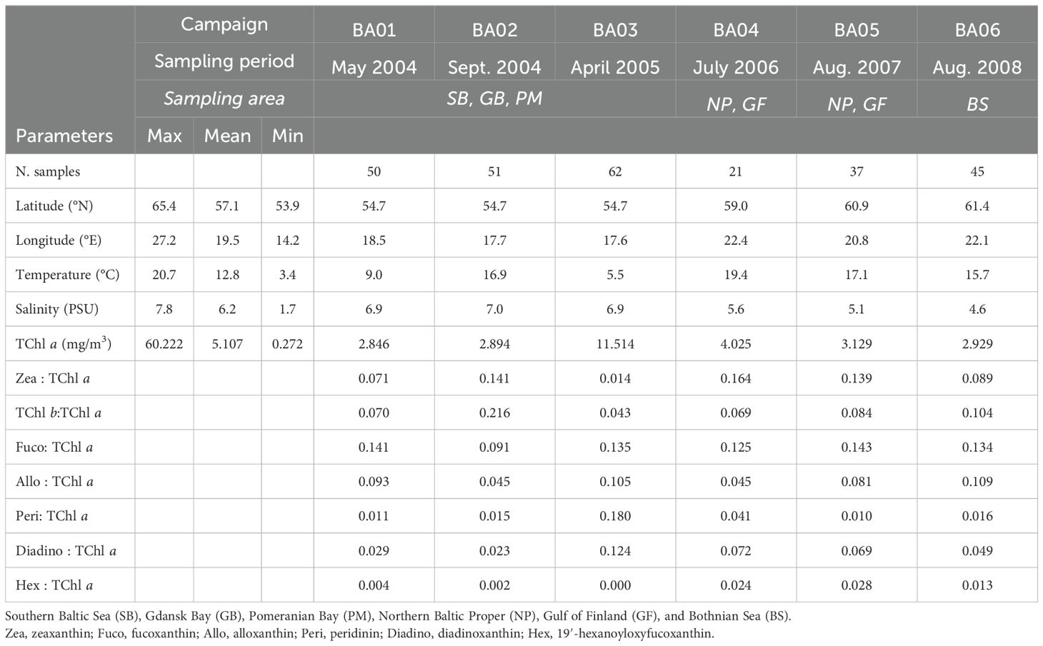
Table 1. Summary of the relevant variables and diagnostic pigments: average TChl a ratios for surface samples of BA01–BA06 campaigns.

In addition to the quality control measures introduced in Section 2.2, the criteria established by Aiken et al. (2009) for evaluating the quality of datasets used in the development of bio-optical algorithms (Hirata et al., 2011) were also applied to ensure internal consistency within each oceanographic campaign. The relationship between log-transformed TChl a and the sum of accessory pigments (TAcc; Trees et al., 2000) was independently verified for each of the six oceanographic campaigns before proceeding with the data analysis and indicated determination coefficients above 0.97 (Supplementary Figure S1).

The multivariate statistical and network analyses on the HPLC datasets were mainly based on the correlation among the pigments of this dataset. Pearson’s coefficient (R values) was selected as the correlation coefficient (Kramer and Siegel, 2019), and the correlation matrix, associated with both absolute concentrations and ratios to TChl a, was calculated for the 16 pigments chosen for further evaluation (Supplementary Figure S2). The ratio correlations, which had a normalized coefficient, were chosen, as they minimized the variance among the pigment concentration magnitude.

3.1 Hierarchical cluster analysis

The pigments used for the hierarchical clustering were the 16 selected from the HPLC dataset (see Section 2.2). In the present study and in agreement with Catlett and Siegel (2018), the addition of Caro did not significantly change the cluster assignment in the HCA.

The hierarchical cluster analysis of the BA dataset illustrated the presence of five distinct groups of phytoplankton pigments that significantly influence the co-variability of the dataset (Figure 2). These dominant groups were diatoms, dinoflagellates, haptophytes, green algae, and cyanobacteria. Within the mixed nano-phytoplankton community, three sub-clusters were identified: haptophytes, a combination of cryptophytes of dinophyta, and green algae. The identification of the haptophyte community cluster was based on observations of But, Hex, and TChl c3. This pigment group was believed to represent a haptophyte community based on previous observations during early spring and late autumn blooms in the Baltic Sea (Blanz et al., 2005; Hällfors, 2004). The pigments Neo, Lut, and Viola were predominantly associated with green algae, with Viola specifically found in the euglenophytes. A third cluster, including Allo, representative of the red algae, and Peri, characteristic of dinophyta, suggested the coexistence of cryptophytes and dinophyta in the nano-size fraction. It was noteworthy that there was a substantial linkage distance between these clusters and Zea, TChl b, and Fuco. Based on previous findings (Vidussi et al., 2001), Fuco was assumed representative of all diatoms (microfraction), while Zea and TChl b were considered representative of the pico-eucaryote fraction (cyanobacteria).

Figure 2

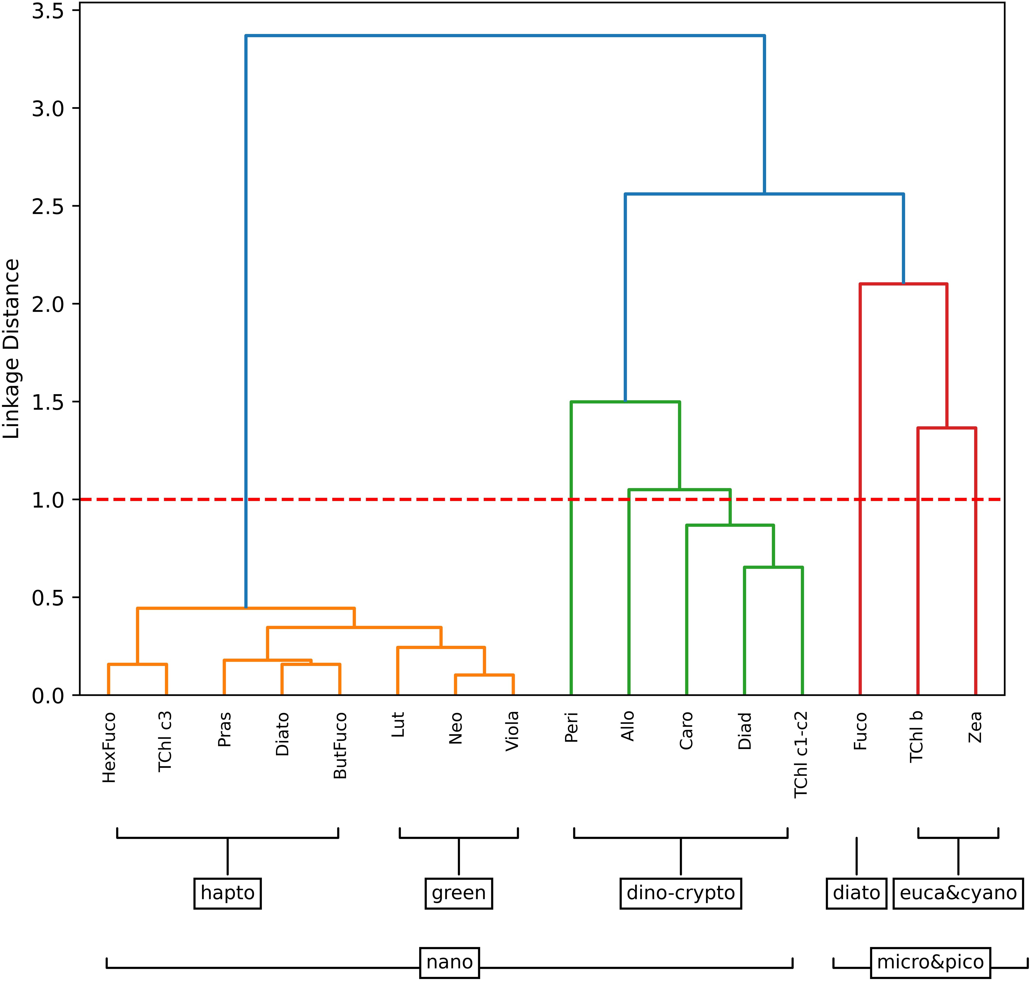
Figure 2. Hierarchical clustering of phytoplankton pigment ratios to TChl a for the Baltic dataset. The major pigment communities (micro-, nano-, and pico-phytoplankton) are identified based on a linkage distance cutoff of 1.0 (red dashed line). The suggested phytoplankton cell size classes for each group are delineated with brackets.

Previous studies (Stoń-Egiert et al., 2010; Stoń-Egiert and Ostrowska, 2022) in the southern Baltic region have identified the dominance of various phytoplankton groups recognizable in our cluster analysis, including cyanobacteria, Dinophyceae, Cryptophyceae, Chlorophyceae, and Euglenophyceae.

A separate analysis was performed for each campaign (Supplementary Figure S3). The prevalence of Fuco and Zea, which are indicative of Euglenophyceae, was most pronounced during campaign B05, which extensively covered the Gulf of Finland. In the first three campaigns conducted in spring (BA01 and BA03) and early autumn (BA02) that were dedicated to the Southern Baltic Sea, Pomeranian Bay, and Gdansk Bay, Fuco was in a separate and dominant cluster, suggesting the dominance of diatoms in this area. The 2010 study by Stoń-Egiert, conducted on phytoplankton pigment data and microscopy samples collected during 12 campaigns in the Southern Baltic Sea and Gdansk Bay regions between 1999 and 2005, confirmed that diatoms are the primary components of phytocenoses in this area of the Baltic Sea. The proportion of Dinophyceae in the total biomass ranged from 7.5% in autumn within the gulfs to 59.2% in early summer in the open Baltic. The contribution of diatoms to the total phytoplankton biomass in early summer in open waters was 23.5%.

3.2 Principal component analysis

The composition of the phytoplankton community was evaluated via a PCA on the phytoplankton pigment concentrations, which were normalized by TChl a concentration. PCA, combined with HCA, enabled us to establish connections among the identified groups and the spatiotemporal variations observed in the BA dataset. The eigenvector loadings for the most influential PCA modes are displayed in a bar plot (Figure 3). We examined the amplitude function (AF) associated with every mode. The amplitude function, as previously utilized by Anderson et al. (2008), served as an indicator of the community structure pattern intensity in both spatial and temporal dimensions (Figure 3). When the AF values were near zero, it indicated that the PCA mode was less important for the current time and location. The present study examined the leading quartile of modes for evaluating community composition in the BA dataset, as they collectively explained 67.4% of the community structure’s variability. Our observations of the first two modes’ high variability were akin to the results by Kramer et al. (2020) on a dataset with a comparable number of observations collected during four oceanographic campaigns in the North Atlantic Ocean. However, the distinctive features of the Baltic Sea, including a high presence of humic acids from rivers, were likely to result in greater variability within the dataset than would be observed in more homogeneous aquatic systems, such as the North Atlantic Ocean. In Mode 1 (Figure 3A), which accounts for 29.3% of the variance, there was a strong positive correlation between TChl c1–c2 associated with dinoflagellates and cryptophytes. Conversely, pigments associated with green algae, cyanobacteria (Zea), and pico-phytoplankton exhibited a strong negative correlation with Mode 1. The spatial distribution showed negative patterns associated with cyanobacteria at mid-range latitudes and positive patterns associated with dinoflagellates at southern latitudes, thereby supporting this interpretation. Mode 2 (Figure 3B) explained 17.5% of the dataset variance and was positively correlated with pigments related to diatoms (Fuco) and haptophytes and moderately correlated with cyanobacteria. Mode 3 (Figure 3C) was negatively correlated with cyanobacteria and strongly correlated with green algae and nano-fraction pigments. Finally, PCA Mode 4 explained 9.5% of the total variance and was negatively correlated with nearly all pigments except Fuco and But, which served as markers for diatoms. Mode 4 (Figure 3D) indicated a dominance of diatoms when the amplitude function was positive and was specifically found in the Gulf of Finland. This result suggests that Mode 4 has the potential to separate diatoms from other groups. Furthermore, this mode showed a negative correlation with all other groups. The PCA suggested a similarity with one aspect of the HCA, namely, the prevalence of diatoms in campaigns BA01–03. However, identifying the dominant community was not consistently possible. In the HCA, TChl b was associated mostly with pico-fraction, while in the PCA, TChl b was more correlated with the green algae, in terms of variations.

Figure 3

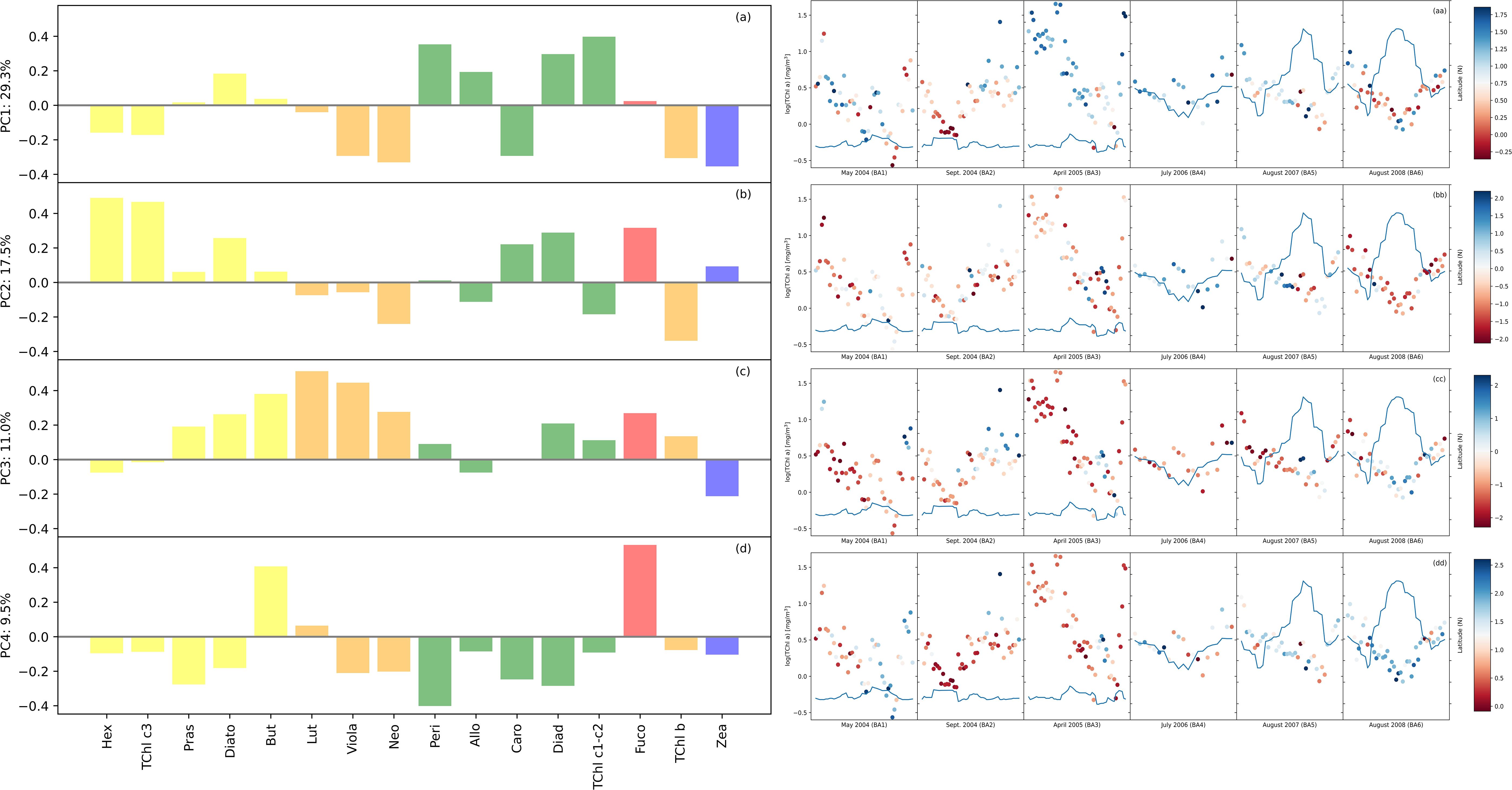
Figure 3. The loadings corresponding to the principal component modes are shown in panels (A–D) for the Baltic dataset. The pigment order was the same as that for the hierarchical cluster analysis (HCA) to facilitate comparisons. The model number is shown above each plot, together with the percentage of variance explained by that mode. The loadings are color-coded based on the main taxonomic groupings: blue for cyanobacteria-pico, red for diatoms-micro, orange for green algae-nano, green for haptophytes-dinoflagellates-nano, and orange for euglanophytes-nano. In panels (aa), (bb), (cc), and (dd) corresponding to each mode are presented the amplitude function (positive in blue and negative in red) corresponding to the log_{TChl a} concentration (scale left side) by each campaign. The latitude is represented by the continuous line on each plot (scale right side).

3.3 Network-based community detection analysis

The Louvain partition method (Dugué and Anthony Perez, 2015; Traag et al., 2019) was utilized to identify the phytoplankton communities within the BA dataset network by optimizing its modularity. Modularity acts as a metric for differentiating intra-community connections. In the case of the pigment ratio network of the BA HPLC dataset, the modularity score reached 0.4. This emphasized the significant similarity observed among samples grouped within the same community and denoted a robust differentiation between various community types using this approach.

The employed network-based method for detecting communities successfully revealed the existence of five prominent phytoplankton pigment communities. To determine the taxonomic classification of each major phytoplankton pigment community, we assessed the mean pigment-to-TChl a ratio of five key biomarker pigments for each community (Table 2). The most relevant community exhibited the highest average Zea ratios, indicating elevated concentrations of picoplankton and cyanobacteria, which were predominant across most of the stations. The second community registered the highest average Fuco ratio. In the third community, the highest ratio of TChl b was detected, typically associated with green algae. The fourth community known for the highest Peri ratio was representative of dinoflagellates. Lastly, the fifth group presented the highest Allo ratio, which was considered representative of the Cryptophyta (nano-fraction). The classification attained through community analysis was subsequently compared with the one derived from the implementation of the Phytoplankton Functional Types (PFTs) algorithm on the Baltic Sea dataset (Brewin et al., 2010; Hirata et al., 2011; Meler et al., 2020) that partially confirmed the results of the network-based analysis. The equations used for the PFT calculations are summarized in Table 2. It has to be recalled that one of the assumptions of the PFT model is that the diagnostic pigments sum (ΣDP) is considered equal to TChl a. It has to be noticed that, while in the PFT classification, TChl b was assigned to two different groups (i.e., green algae and Pico-eukaryotes); in the network-community classification, the partition with predominance of TChl b was assigned to green algae; consequently, in network-community classification, no pico-eukaryote fraction was present. In the PFT classification, Allo was considered only within the nanoplankton size class, while no functional group was associated specifically with cryptophytes. These are the main differences that could be found between the network-community partition and the PFT approach. Ultimately, it is noteworthy that, adhering to the PFT analysis, no station was identified as dominated by haptophyte PFT.

Table 2

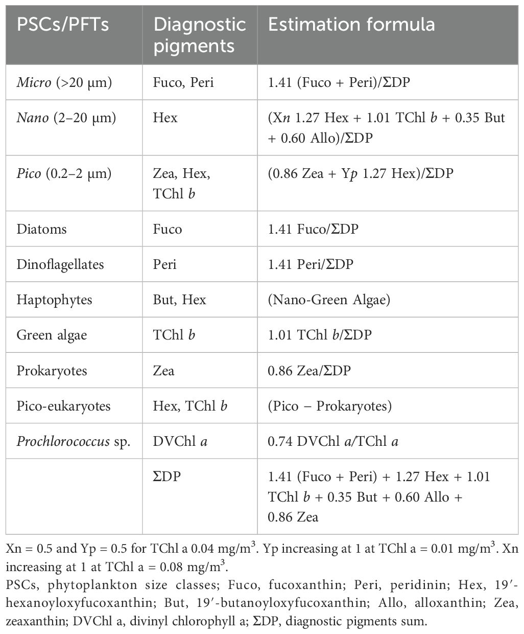
Table 2. Phytoplankton functional types (PFTs), diagnostic pigments, and their taxonomic association.

The spatiotemporal arrangement of the samples in the NCA (Figure 4A) illustrated that dinoflagellate and diatom communities were predominantly present in the Baltic Sea with a significant concentration observed in the Southern Baltic Sea and Gdansk Bay. Notably, the prevalence of these two communities varied with the changing seasons. However, prokaryotic and pico-eukaryotic communities were distributed over a wider range of latitudes, including different temperature and salinity conditions. Comparing the outcomes of the NCA with the communities identified through PFT analysis (Figure 4B), a remarkable similarity in the spatiotemporal distribution of the samples within each community was observed for all the campaigns except for the BA02 and BA05 campaigns. For the BA02 campaign, the PFT analysis assigned part of the stations to the pico-eucaryotes instead of to the cryptophytes, and in the BA05 campaign, the NCA identified no diatoms among the sampling stations, while the PFT analysis did. Moreover, the number of samples assigned to each community was quite consistent, except for diatoms (Supplementary Table S1). To enhance the differentiation of communities identified by PCA, the results of the PCA were integrated with the communities recognized through the NCA (Figure 5). Comparing the amplitude function of the first two modes, we can separate the pico-eucaryote community in the case of the NCA, while the outcome was not so evident in the case of the PFT application, where the pico-eucaryotes were mixed with diatoms. Similarly, the dinoflagellate community looks better isolated in the NCA than in the PFT.

Figure 4

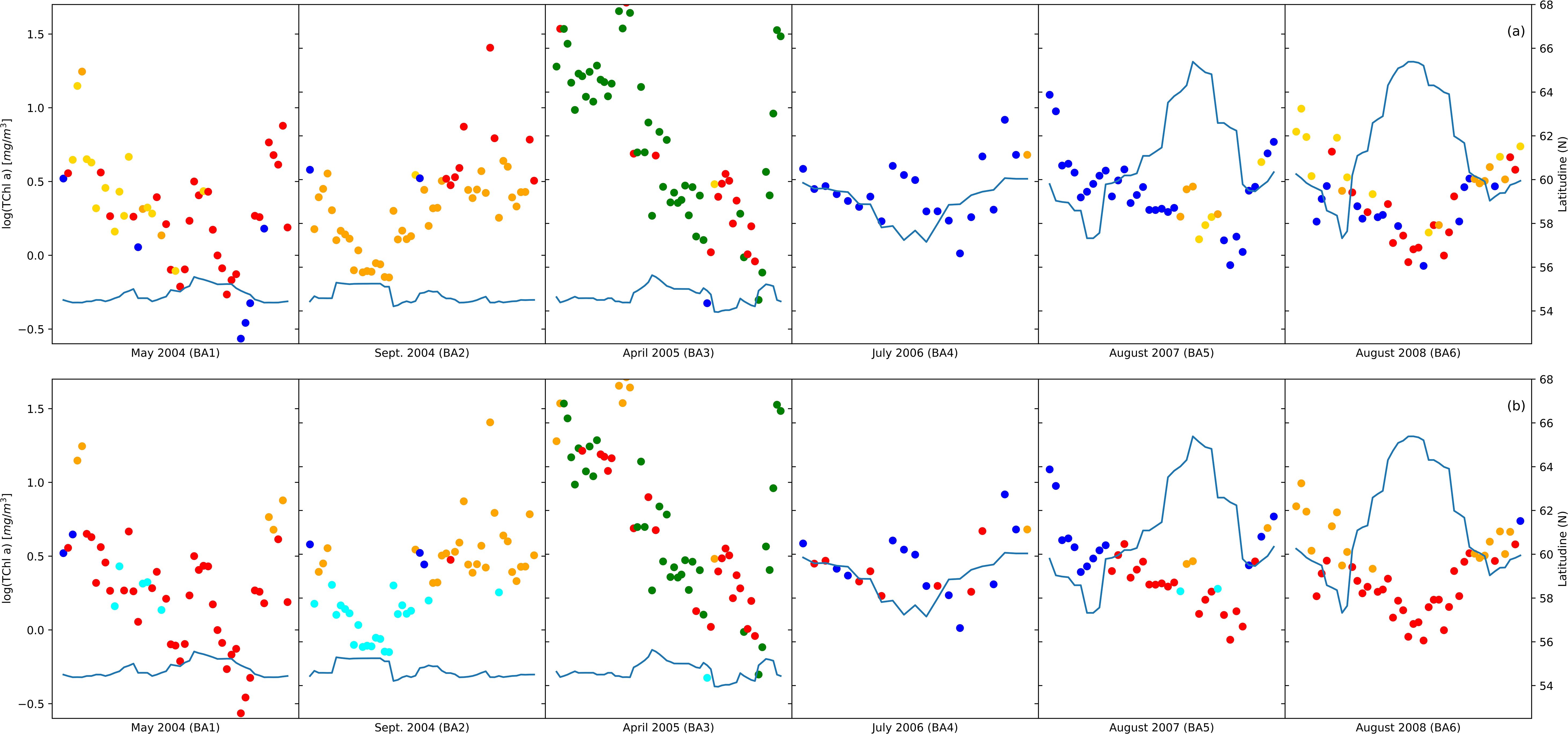
Figure 4. The group distribution from network analysis (A) compared with phytoplankton functional type (PFT) distribution (B). Colors indicate major taxonomic groups: diatoms (red), dinoflagellates (green), green algae (orange), Prokaryotes (cyan), pico-eucaryotes (blue), and cryptophytes (gold); the continuous line indicates the latitude (left axis) and the position related to TChl a concentration (right axis).

Figure 5

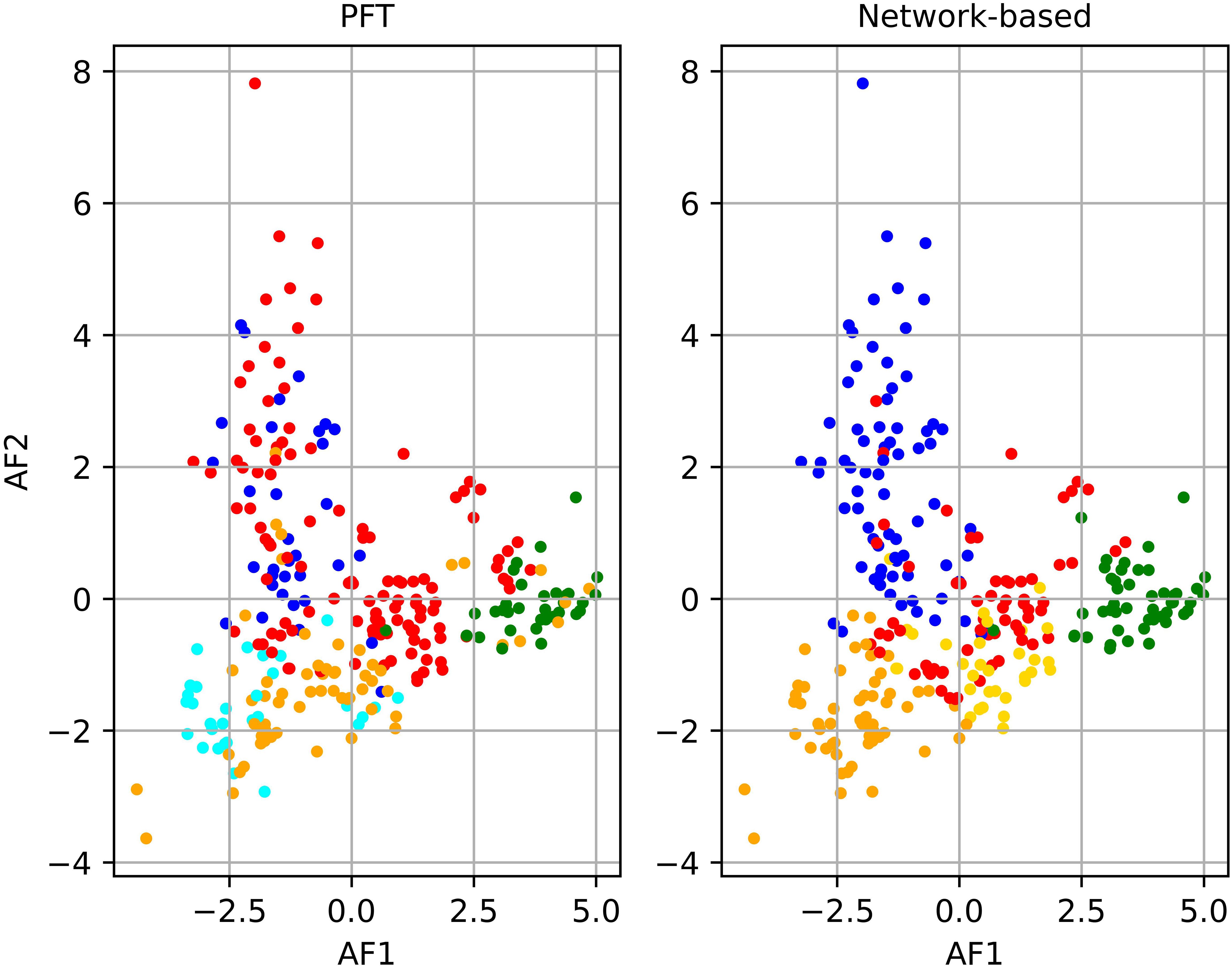
Figure 5. Principal component analysis (PCA) compared to network partitioning results (shown in color): diatoms (red), dinoflagellates (green), green algae (orange), Prokaryotes (cyan), pico-eucaryotes (blue), and cryptophytes (gold).

In network analysis, particularly in ecological studies, understanding the underlying structure and relationships within a community is crucial. One method to achieve this is through the computation of a minimum spanning tree (MST). The outcomes of a spanning tree resulting from a matrix modularity analysis can provide insights into the community structure and relationships within the phytoplankton community as well, revealing hierarchical or structural aspects of the network (Supplementary Figure S4). In terms of community detection, this could indicate that the central community played a more significant role or stronger connections with other communities compared to the peripheral community. In our case, the community (2) that dominated the center was the one with predominant Allo pigments. This was interpreted as the dominance of cryptophytes. At the center, the network showed more nodes and denser connections, while the sparser community in the peripheral [community (0)] was dominated by TChl b. However, it should be noticed that the other three communities—Prokaryotes, dinoflagellates, and diatoms—were widespread among the leaf, in between the center and the peripheral, thus suggesting the cross-diffusion of these pigments among various phytoplankton species present in the Baltic Sea.

We compared the results of machine learning analysis with the outcome of the CHEMTAX (Mackey et al., 1996) community classification. As the initial input of the CHEMTAX matrix, we used the pigment ratios developed for the southern Baltic (Schlüter et al., 2000). As the southern Baltic populations could not be considered representative of the whole basin, we established a different matrix for each campaign (Supplementary Figure S5) considering each campaign belonging to a separate cluster. However, the ratios used in the generated matrix applied to the Northern and Central Baltic campaigns were not verified by microscopy counts, thus lacking robustness. Applying CHEMTAX to our dataset and accordingly to the matrix used for the community identification, we obtained information on seven groups (Dinophyceae, Diatoms, Cryptophytes, Cyaonophytes, Chlorophyceae, Euglenophytes, and Prasinophytes) instead of the five identified through our statistical approaches. According to the CHEMTAX analysis, the cryptophytes’ fraction dominated in three campaigns (BA01, BA03, and BA05), and this partially confirmed the analysis through the network community. However, the cyanobacteria were present in a smaller fraction of stations, while in all other analyses, they were predominant in the BA05 and BA06 campaigns. The diatoms, which are the most representative community according to the PFT analysis, are present in percentages lower than 17%.

4 Discussion

The present study examined the surface phytoplankton community distribution in the Baltic Sea, derived from HPLC datasets covering different seasons and different areas of the Baltic Sea. The dataset underwent different statistical analyses to assess the phytoplankton community composition based on the predominance of diagnostic pigments representative of a phytoplankton group or species.

In the Baltic Sea, the typical seasonal cycle of phytoplankton species succession follows a well-established pattern. When comparing our results with previous findings, the BA cruises reflected this seasonal progression of phytoplankton communities. A spring diatom bloom and a mid-summer cyanobacterial bloom were followed by a late summer to autumn peak of haptophytes and dinoflagellates. In the BA campaigns, spring and early summer cruises showed an abundance of samples from the diatom community, coinciding with the spring phytoplankton bloom. Stoń-Egiert et al. (2010) reported that diatoms accounted for approximately 50% of the total phytoplankton biomass in the Gdansk Bay in spring and that the composition of the phytoplankton community varied with increasing distance from the river mouth, with a notable presence of dinophytes (ranging from 10% in the vicinity of the river mouth to 40% in more distant regions of the Gulf). The aforementioned studies have demonstrated the presence of diatoms (Fuco pigment) in the initial BA01–03 campaigns that focused on the Southern Baltic Sea and Gdansk Bay. Both the analysis by single campaign and a combined analysis of these datasets have shown the presence of green algae during this period. In early summer, dinoflagellates became an important part of the community alongside diatoms. The transition from late summer to early autumn (BA05–06 and B04, respectively) was dominated by samples from the haptophyte community, with some cyanobacteria present as the bloom wanes. These results are in agreement with previous findings on cyanobacteria cycle in the Baltic Sea.

Conventional pigment-based methods such as CHEMTAX assume linear independence of pigments and require pre-defined knowledge of pigment contributions to individual phytoplankton groups. In the context of the Baltic Sea study, the dataset’s collinearity and dynamic conditions challenge the linear independence of pigment assumptions, making the methods used here more suitable for capturing the phytoplankton community composition. In our initial data analysis, we applied different statistical tools and unsupervised machine learning techniques, including HCA, PCA, and NCA, to the HPLC dataset. The aim was to assess the consistency and coherence of the results derived from these analyses. To validate the robustness of our chemotaxonomic data analysis, we compared the outcomes with alternative models and algorithms commonly used in characterizing chemotaxonomic composition (PFT). Additionally, we cross-referenced our findings with results from prior studies conducted in the Baltic region.

TChl b is a pigment present in Euglenophyta, Chlorophyta, and Prasinophytes, and, as DVChl b, can contribute to pico-eukaryotes (Supplementary Table S1). In the HCA, TChl b clustered with Zea but not with other pigments representative of green algae (i.e., Pras, Lut, Neo, and Viol). This suggested that TChl b primarily contributed to the pico-eukaryote fraction rather than to green algae. However, in the PCA, TChl b followed the behavior of Neo and Viol in all four modes and Lut in the first three modes, while Pras followed a distinctive path compared to TChl b in the first two modes. The PCA interpretation suggested that TChl b is associated as a biomarker pigment with green algae since it follows the path of other pigments commonly present in green algae. The distinctive behavior of Pras in the first two modes can be interpreted as a characteristic of Prasinophytes, distinguishing the Prasinophytes from the other green algae. In the NCA, and similarly to the PCA outcome, the community linked to TChl b was composed predominantly of green algae pigments, while Zea is associated with a different community. In light of these considerations, the HCA clustering appears to be the least explanatory regarding both TChl b and green algae. Ultimately, the cryptophytes were not clearly identified in either the HCA or PCA, while in the NCA, a community associated with Allo was identified.

In the NCA, the initial step was the analysis of the adjacency correlation matrix, which evidenced the presence of five areas of strong correlation. The network was employed to identify communities through the Louvain partition method. This revealed a modularity value above 0.3 (0.39 in our case), indicating a significant level of community interconnectedness, as noted by Newman (2006), where significant interconnectedness within a community indicated that the population assigned to each community had many common traits. We also examined whether the communities identified through network analysis corresponded with those identified using other methods such as PCA and HCA, with the limitation mentioned above regarding TChl b for HCAs. In the network analysis, we assigned each sample to a specific community in the network-based community detection analysis, thus allowing us to consider the spatiotemporal distribution of the five communities. The principal phytoplankton community identified by PCA was composed of diatoms, dinoflagellates, cyanobacteria, cryptophytes, and green algae, which was consistent with the results of the network analysis (Supplementary Figure S6). Upon comparison of HCA with the network analysis, a notable distinction was raised: HCA failed to assign a specific cluster to TChl b, whereas the NCA recognized TChl b as representative of a distinct community. Furthermore, the presence of Zea was identified differently in each analysis, with network analysis highlighting as a key feature. It is worth noticing that, while PCA and HCA offer an overarching perspective of the dataset, the network analysis discreetly assigns a dominant phytoplankton community to each station. Therefore, it appeared more beneficial to compare the results of network analysis with PFT analysis, which similarly assigns a dominant community to each observation (Figures 4, 5). Comparing the two methodologies, the difference between NCA and PFT analysis was more evident for the BA02 and BA06 campaigns. If in BA02 we compare the outcome of the PFT with the NCA, the PFT assigned 22 stations to pico-eucaryotes whether the NCA assigned them to cryptophytes: considering the season and the temperature condition (Table 1 and Figure 6), these 22 stations are more likely to associate these stations with cyanobacteria (i.e., PFT assignment). In the case of B02, the PFT assignment is more coherent with the environmental conditions. Conversely, in BA06, the PFT assigns to the diatom community the stations that, for the environmental conditions (temperature and season), are more likely to be representative of a Prokaryotes dominance (NCA assignment). In B06, the station assignment to the phytoplankton group of NCA has to be preferred to the PFT. Overall, it has to be recognized that a limit of this approach was that in the network analysis—and the PFT analysis—each sample was associated with a specific category (color) discretely, whereas reality is more complex than clear-cut categories. In addition, the PCA proved to be a valuable tool in analyzing seasonal variations in phytoplankton composition. The two approaches, PCA and NCA, could be complementary to develop a holistic view of the dataset.

Figure 6

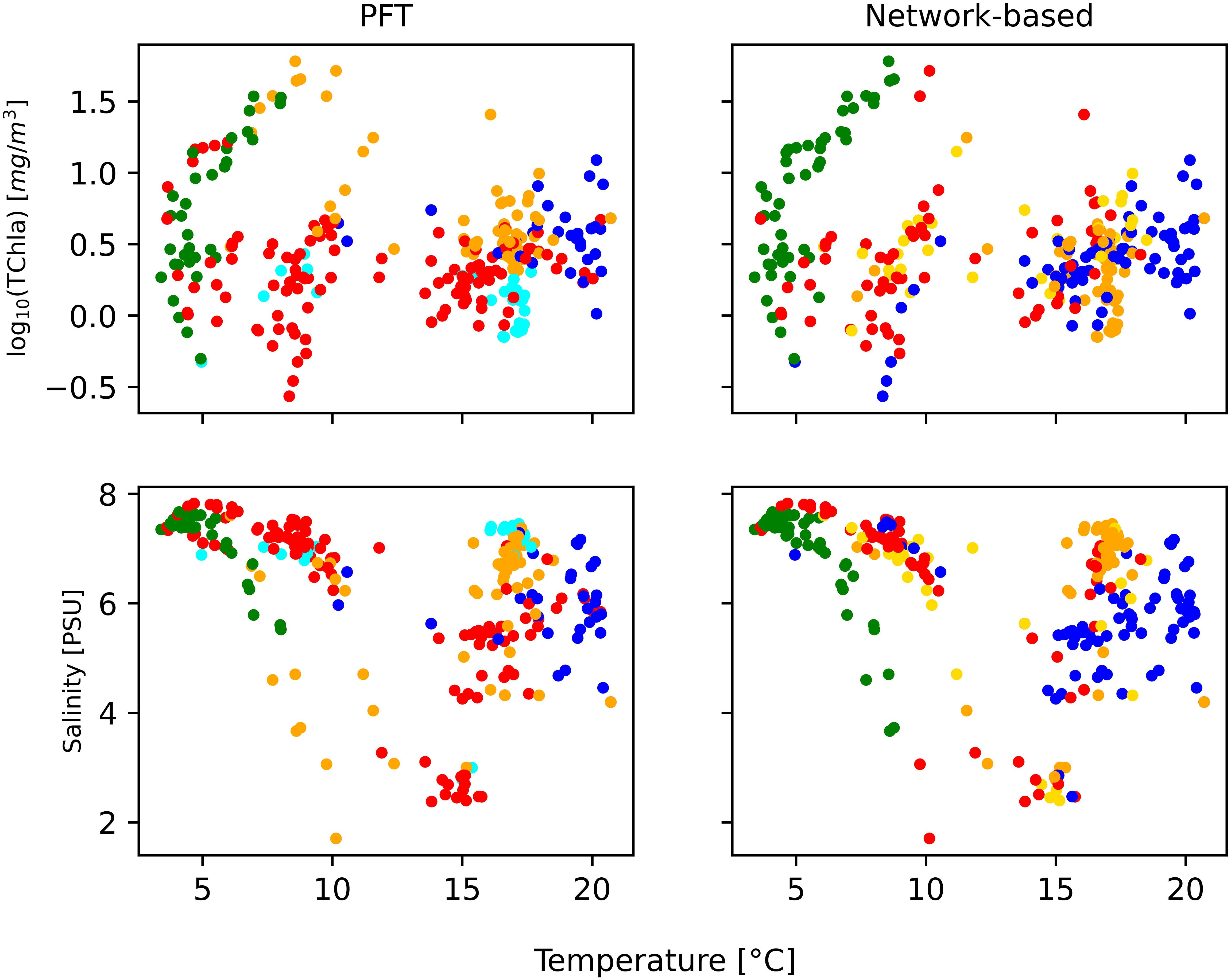
Figure 6. Regression of physical parameter temperature and salinity for phytoplankton functional type (PFT) analysis and network-based analysis, all colored with the dominant community [diatoms (red), dinoflagellates (green), green algae (orange), Prokaryotes (blue), pico-eucaryotes (cyan), and cryptophytes (gold)].

We extended our comparison between PFT and network analysis to hydrological conditions that can influence the observed variability in phytoplankton community structure, such as temperature and salinity (Table 3). A parallel analysis using the PFT algorithm yielded similar conclusions (Figure 6). In this context, the spatiotemporal distribution of phytoplankton communities inferred from HPLC pigments in the Baltic Sea through network analysis aligned well with the phytoplankton community composition that was found in previous analyses (Stoń-Egiert et al., 2010; Stoń-Egiert and Ostrowska, 2022), evidencing the presence of cyanobacteria at higher temperature and salinity (Pliński et al., 2007).

Table 3

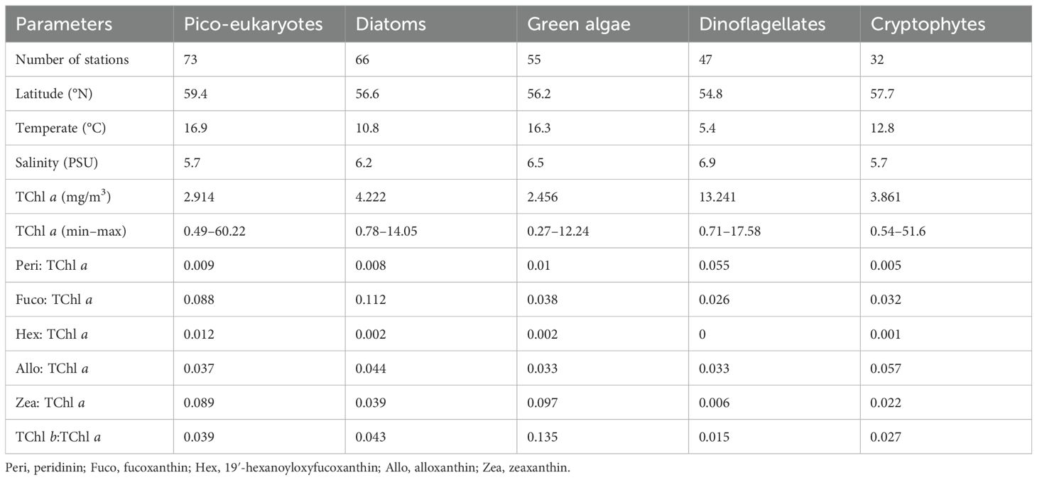
Table 3. Summary of the relevant variables and averaged diagnostic pigments: TChl a ratios resulting from network-based analysis.

Our data-driven statistical analyses on the HPLC pigment dataset were able to identify five distinct taxonomically defined phytoplankton communities in the Baltic Sea, characterized by five biomarker pigments: diatoms (Fuco), dinoflagellates (Peri), cryptophytes (Allo), green algae (TChl b), and cyanobacteria-pico-plankton (Zea). Notably, dinoflagellates were found to be distinct from diatoms in this regional context, a differentiation that was not commonly observed globally (Kramer and Siegel, 2019). Samples from the six BA cruises had sufficient concentrations of dinoflagellate pigments to allow for their clear separation from diatoms and other red algal pigments in PCA and network-based community detection. However, this distinction was less clear in a hierarchical cluster analysis.

5 Conclusion

In our investigation, we used multivariate statistics and unsupervised and supervised machine learning methods to analyze a diverse dataset of HPLC pigment observations obtained from Baltic Sea surface samples. We aimed to extract key insights from these pigment observations, considering various spatial and temporal dimensions as well as available hydrological variables. We addressed the selection process of appropriate statistical methods and underscored the importance of the data quality of the pigment dataset. We also performed a comparative analysis, comparing our results with those of alternative models and algorithms commonly employed to characterize chemotaxonomic composition, such as PFTs and CHEMTAX. Additionally, we compared our results with findings from previous studies conducted in the Baltic Sea region (Wasmund et al., 2011; HELCOM, 2018).

Our findings suggested that the network-based community identification alongside PCA on the HPLC dataset holds promise for effective interpretation of phytoplankton community composition. This combined approach demonstrated the potential to identify phytoplankton communities, even within the complexities of basins such as the Baltic Sea. However, it has to be acknowledged that the data-driven statistical analyses employed in this study had some limitations. In particular, pigment-based methods are bound by the specific conditions under which the data were collected. In all these approaches, we referred to the diagnostic pigments or to the known pigment ratios to reconstruct the phytoplankton community. As has been already remarked by Meler et al. (2020), all these approaches, based on diagnostic pigments, are simplified with statistical error in the order of 20%. A step forward in the research is integrating the analysis of the pigment dataset with concomitant measurements of optical features. Ultimately, these methods did not directly measure phytoplankton biomass or productivity, which limited both the derived phytoplankton communities and the potential development of satellite algorithms. Despite these limitations, the insights gained from these methods offered valuable metrics and datasets that can contribute to both current and future advances in remote sensing technologies.

Data availability statement

The raw data supporting the conclusions of this article will be made available by the authors, without undue reservation.

Author contributions

EC: Conceptualization, Data curation, Formal Analysis, Investigation, Methodology, Validation, Visualization, Writing – original draft, Writing – review & editing. AP: Writing – review & editing.

Funding

The author(s) declare financial support was received for the research, authorship, and/or publication of this article. The study has been supported by the European Commission Directorate General Joint Research Centre (JRC) and the Copernicus Program.

Acknowledgments

The author would like to acknowledge Juha Flinkman, Seppo Kaitala, and Jukka Seppälä from the Finnish Environment Institute (formerly Finnish Institute of Marine Research) for the opportunity to participate in the oceanographic campaign onboard the R/V Aranda and the crew of R/V Aranda for their support during all the cruises. Acknowledgments are due to Dirk Van der Linde from JRC for water sampling and laboratory analyses.

Conflict of interest

The authors declare that the research was conducted in the absence of any commercial or financial relationships that could be construed as a potential conflict of interest.

Publisher’s note

All claims expressed in this article are solely those of the authors and do not necessarily represent those of their affiliated organizations, or those of the publisher, the editors and the reviewers. Any product that may be evaluated in this article, or claim that may be made by its manufacturer, is not guaranteed or endorsed by the publisher.

Supplementary material

The Supplementary Material for this article can be found online at: https://www.frontiersin.org/articles/10.3389/fmars.2024.1425347/full#supplementary-material

Supplementary Figure 1 | The log-log co-variance TAcc/TChl a along the six Baltic Oceanographic Campaigns, axis in log scale (mg m^-3).

Supplementary Figure 2 | The correlation matrix (Pearson correlation coefficient) is associated with both absolute concentrations (bottom left) and ratios to TChl a(top right), for the 16 pigments.

Supplementary Figure 3 | Hierarchical clustering of phytoplankton pigment ratios to TChl a for each campaign of the Baltic dataset.

Supplementary Figure 4 | Spanning tree resulting from a matrix modularity analysis: Green Algae (community 0), Procaryotes (community 1), Cryptophytes (community 2), Dinoflagellates (community 3), Diatoms (community 4)

Supplementary Figure 5 | CHEMTAX applied to the six oceanographic campaigns (initial matrix provided in Schlüter et al., 2000). In the pies the relative biomass abundance correspond to Dinophycacee (blue), Diatoms (orange), Cryptophytes (green), Cyaonophytes (red), Chlorophyceae (purple), Euglenophytes (brown) and Prasinophytrs (pink)

References

Aiken J., Pradhan Y., Barlow R., Lavender S., Poulton A., Holligan P., et al. (2009). Phytoplankton pigments and functional types in the Atlantic Ocean: A decadal assessment 1995-2005. Deep Sea Res. Part II: Topical Stud. Oceanography 56, 899–917. doi: 10.1016/j.dsr2.2008.09.017

Crossref Full Text | Google Scholar

Allocco D. J., Kohane I. S., Butte A. J. (2004). Quantifying the relationship between co-expression, co-regulation, and gene function. BMC Bioinf. 5, 18. doi: 10.1186/1471-2105-5-18

Crossref Full Text | Google Scholar

Anderson C. R., Siegel D. A., Brzeniski M. A., Guillocheau N. (2008). Controls on temporal patterns in phytoplankton community structure in the Santa Barbara Channel, California. J. Geophys. Res. 113, C04038. doi: 10.1029/2007JC004321

Crossref Full Text | Google Scholar

Axe P., Sahlsten E. (2001). “Hydrografi/hydrokemi,” in Bottniska viken 2001. (Umeå: Research Center of Umeå University). Available at: http://www.havet.nu/dokument/Bv2001hydro.pdf.

Google Scholar

Barrón R. K., Siegel D. A., Guillocheau N. (2014). Evaluating the importance of phytoplankton community structure to the optical properties of the Santa Barbara Channel, California. Limn. Oceanogr. 59, 927–946. doi: 10.4319/lo.2014.59.3.0927

Crossref Full Text | Google Scholar

Blanz T., Emeis K., Siegel H. (2005). Controls on alkenone unsaturation ratios along the salinity gradient between the open ocean and the Baltic Sea. Geochim. Cosmochim. Acta 69, 3589–3600. doi: 10.1016/j.gca.2005.02.026

Crossref Full Text | Google Scholar

Blondel V., Guillaume J.-L., Lambiotte R., Lefebvre E. (2008). Fast unfolding of communities in large networks. J. Stat. Mechanics Theory Exp. 2008. doi: 10.1088/1742-5468/2008/10/P10008

Crossref Full Text | Google Scholar

Bracher A., Taylor M. H., Taylor B., Dinter T., Rottgers R., Steinmetz F. (2015). Using empirical orthogonal functions derived from remote-sensing reflectance for the prediction of phytoplankton pigment concentrations. Oc. Sci. 11, 139–158. doi: 10.5194/os-11-139-201

Crossref Full Text | Google Scholar

Brewin R. J. W., Sathyendranath S., Hirata T., Lavender S. J., Barciela R. M., Hardman-Mountford N. J. (2010). A three-component model of phytoplankton size class for the Atlantic. Oc. Ecol. Model. 221, 1472–1483. doi: 10.1016/j.ecolmodel.2010.02.014

Crossref Full Text | Google Scholar

Canuti E. (2023). Phytoplankton pigment in situ measurements uncertainty evaluation: an HPLC interlaboratory comparison with a European-scale dataset. Front. Mar. Sci. 10. doi: 10.3389/fmars.2023.1197311

Crossref Full Text | Google Scholar

Canuti E., Artuso F., Bracher A., Brotas V., Devred E., Dimier C., et al. (2022). The Fifth HPLC Intercomparison on Phytoplankton Pigments (HIP-5) Technical Report (Luxembourg: Publications Office of the European Union). EUR 31334 EN. doi: 10.2760/563102

Crossref Full Text | Google Scholar

Canuti E., Ras J., Grung M., Röttgers R., Costa Goela P., Artuso F., et al. (2016). HPLC/DAD Intercomparison on Phytoplankton Pigments (HIP-1, HIP-2, HIP-3 and HIP-4) (Luxembourg: Publications Office of the European Union). EUR 28382 EN.

Google Scholar

Catlett D., Siegel D. A. (2018). Phytoplankton pigment communities can be modeled using unique relationships with spectral absorption signatures in a dynamic coastal environment. J. Geophys. Res.: Oc. 123, 246–264. doi: 10.1002/2017JC013195

Crossref Full Text | Google Scholar

Dugué N., Anthony Perez A. (2015). Directed Louvain: maximizing modularity in directed networks (Université d’Orléans). Available at: https://hal.archives-ouvertes.fr/hal-01231784.

Google Scholar

Hagberg A., Swart P., Schult D. (2008). NetworkX: High Productivity Software for Complex Networks (Los Alamos National Laboratory (LANL). Available at: https://networkx.org/.

Google Scholar

Hällfors G. (2004). “Checklist of Baltic Sea phytoplankton species (including some heterotrophic protistan groups),” in Baltic Marine Environment Protection Commission (Helsinki Commission). Available at: https://www.helcom.fi/wp-content/uploads/2019/10/BSEP95.pdf.

Google Scholar

HELCOM. (2018). “State of the Baltic Sea – Second HELCOM holistic assessment 2011–2016,” in Baltic Sea Environment Proceedings, vol. 155. (HELCOM). Available at: https://helcom.fi/media/publications/BSEP155.pdf.

Google Scholar

Hirata T., Hardman-Mountford N. J., Brewin R. J. W., Aiken J., Barlow R. G., Suzuki K., et al. (2011). Synoptic relationships between surface chlorophyll-a and diagnostic pigments specific to phytoplankton functional types. Biogeosc. 8, 311–327. doi: 10.5194/bg-8-311-2011

Crossref Full Text | Google Scholar

Hooker S. B., Thomas C. S., Van Heukelem L., Schluter L., Ras J., Claustre H., et al. (2010). The Forth SeaWiFS HPLC Analysis Round-Robin Experiment (SeaHARRE-4) (Greenbelt, Maryland: NASA Goddard Space Flight Center). NASA Tech. Memo. 2010-215857.

Google Scholar

Hooker S. B., Heukelem L., Thomas C., Claustre H., Ras J., Barlow R., et al. (2005). The second SeaWiFS HPLC analysis round-robin Eexperiment (SeaHARRE-2) NASA Technical Memorandum. 1-112.

Google Scholar

IOCCG (2014). Phytoplankton Functional Types from Space Vol. 15. Ed. Sathyendranath S. (Dartmouth, Canada: IOCCG).

Google Scholar

Jeffrey S. W., Mantoura R. F. C., Wright S. W. (1997). Phytoplankton Pigments in Oceanography (Paris: UNESCO).

Google Scholar

Kramer S. J., Siegel D. A. (2019). How can phytoplankton pigments be best used to characterize surface ocean phytoplankton groups for ocean color remote sensing algorithms? J. Geophys. Res.: Oc. 124, 7557–7574. doi: 10.1029/2019JC015604

Crossref Full Text | Google Scholar

Kramer S. J., Siegel D. A., Graff J. R. (2020). Phytoplankton community composition determined from co-variability among phytoplankton pigments from the NAAMES field campaign. Front. Mar. Sci. Sec. Mar. Ecosys. Ec. 7. doi: 10.3389/fmars.2020.00215

Crossref Full Text | Google Scholar

Latasa M., Bidigare R. R. (1998). A comparison of phytoplankton populations of the Arabian Sea during the Spring Intermonsoon and Southwest Monsoon of 1995 as described by HPLC-analyzed pigments. Deep Sea Res.Part II: Topical Stud. Oceanography 45, 2133–2170. doi: 10.1016/S0967-0645(98)00066-6

Crossref Full Text | Google Scholar

Lotze H. K., Lenihan H. S., Bourque B. J., Bradbury R. H., Cooke R. G., Kay M. C., et al. (2006). Depletion, degradation, and recovery potential of estuaries and coastal seas. Science 312, 1806–1809. doi: 10.1126/science.1128035

PubMed Abstract | Crossref Full Text | Google Scholar

Mackey M., Mackey D., Higgins H. W., Wright S. W. (1996). CHEMTAX - a program for estimating class abundances from chemical markers: Application to HPLC measurements of phytoplankton. Mar. Ecol. Prog. Ser. 144, 265–283. doi: 10.3354/meps144265

Crossref Full Text | Google Scholar

Mason M. J., Fan G., Plath K. (2009). Signed weighted gene co-expression network analysis of transcriptional regulation in murine embryonic stem cells. BMC Genomics 10, 327. doi: 10.1186/1471-2164-10-327

PubMed Abstract | Crossref Full Text | Google Scholar

Meler J., Woźniak S. B., Stoń-Egiert J. (2020). Comparison of methods for indirectly estimating the phytoplankton population size structure and their preliminary modifications adapted to the specific conditions of the Baltic Sea. J. Mar. Syst. 212, 103446. doi: 10.1016/j.jmarsys.2020.103446

Crossref Full Text | Google Scholar

Mouw C. B., Hardman-Mountford N. J., Alvain S., Bracher A., Brewin R. J. W., Bricaud A., et al. (2017). A consumer’s guide to satellite remote sensing of multiple phytoplankton groups in the Global Ocean. Front. Mar. Sci. 4. doi: 10.3389/fmars.2017.00041

Crossref Full Text | Google Scholar

Nair M. E. J., Sathyendranath S., Platt T., Morales J., Stuart V., Forget M.-H., et al. (2008). Remote sensing of phytoplankton functional types. Remote Sens. Environ. 112, 3366–3375. doi: 10.1016/j.rse.2008.01.021

Crossref Full Text | Google Scholar

Newman M. E. J. (2006). Modularity and community structure in networks. App. Math 103, 8577–8582. doi: 10.1073/pnas.0601602103

Crossref Full Text | Google Scholar

Olli K., Klais-Peets R., Tamminen T., Ptacnik R., Andersen T. (2011). Long-term changes in the Baltic Sea phytoplankton community. Boreal Env. Res. 16, 3–14.

Google Scholar

Pliński M., Mazur-Marzec H., Józwiak T., Kobos J. (2007). The potential causes of cyanobacterial blooms in Baltic Sea estuaries. Oceanol. Hydrobiol. Stud. 36, 125–137. doi: 10.2478/v10009-007-0001-x

Crossref Full Text | Google Scholar

Rodriguez F., Varela M., Zapata M. (2002). Phytoplankton assemblages in the Gerlache and Bransfield Straits (Antarctic Peninsula) determined by light microscopy and CHEMTAX analysis of HPLC pigment data. Deep-Sea Res. Pt. II 49, 723–747. doi: 10.1016/S0967-0645(01)00121-7

Crossref Full Text | Google Scholar

Roy S., Llewellyn C. A., Egeland E. S., Johnsen G. (2011). Phytoplankton Pigments, Characterization, Chemotaxonomy and Applications in Oceanography (Cambridge, UKCambridge Univ. Press), 845.

Google Scholar

Schmelzer, Seinä N. A., Lundqvuist J.-E., Sztobryn M. (2008). Ice, in State and Evolution of the Baltic Sea, 1952–2005, edited by R. Feistel, G. Nausch, and N. Wasmund. (Wiley, Hoboken, N. J.). pp. 199–240. doi: 10.1002/9780470283134.ch8

Crossref Full Text | Google Scholar

Schlüter L., Behl B., Striebel M., Stibor H. (2016). Comparing microscopic counts and pigment analyses in 46 phytoplankton communities from lakes of different trophic states. Freshw. Biol. 61, 1627–1639. doi: 10.1111/fwb.12803

Crossref Full Text | Google Scholar

Schlüter L., Garde K., Kaas H. (2004). Detection of the toxic cyanobacteria Nodularia spumigena by means of a 4-keto-myxoxanthophyll-like pigment in the Baltic Sea. Mar. Ecol. Prog. Ser. 275, 69–78. doi: 10.3354/meps275069

Crossref Full Text | Google Scholar

Schlüter L., Møhlenberg F., Havskum H., Larsen S. (2000). The use of phytoplankton pigments for identifying and quantifying phytoplankton groups in coastal areas: testing the influence of light and nutrients on pigment/chlorophyll a ratios. Mar. Ecol. Prog. Ser. 192, 49–63. doi: 10.3354/meps192049

Crossref Full Text | Google Scholar

Seppälä J. (2009). “Fluorescence properties of Baltic sea phytoplankton,” in Monographs of the Boreal environment research, vol. 34. (Edita Prima Ltd, Helsinki), 83.

Google Scholar

Stoń-Egiert J., Łotocka M., Ostrowska M., Kosakowska A. (2010). The influence of biotic factors on phytoplankton pigment composition and resources in Baltic ecosystems: new analytical results. Oceanologia 52, 101–125. doi: 10.5697/oc.52-1.10

Crossref Full Text | Google Scholar

Stoń-Egiert J., Ostrowska M. (2022). Long-term changes in phytoplankton pigment contents in the Baltic Sea: Trends and spatial variability during 20 years of investigations. Cont. Shelf Res. 236, 206–210. doi: 10.1016/j.csr.2022.104666

Crossref Full Text | Google Scholar

Sun X., Shen F., Brewin R. J. W., Li M., Zhu Q. (2022). Light absorption spectra of naturally mixed phytoplankton assemblages for retrieval of phytoplankton group composition in coastal oceans. Limnol. Oceanogr. 67, 946–961. doi: 10.1002/lno.12047

Crossref Full Text | Google Scholar

Traag V. A., Waltman L., van Eck N. J. (2019). From Louvain to Leiden: guaranteeing well-connected communities. Sci. Rep. 9, 5233. doi: 10.1038/s41598-019-41695-z

PubMed Abstract | Crossref Full Text | Google Scholar

Trees C. C., Clark D. K., Bidigare R. R., Ondrusek M. E., Mueller J. L. (2000). Accessory pigments versus chlorophyll a concentrations within the euphotic zone: A ubiquitous relationship. Limnol. Oceanogr. 5, 1130–1143. doi: 10.4319/lo.2000.45.5.1130

Crossref Full Text | Google Scholar

Uitz J., Claustre H., Morel A., Hooker S. B. (2006). Vertical distribution of phytoplankton communities in open ocean: an assessment based on surface chlorophyll. J. Geophys. Res. 111, C08005. doi: 10.1029/2005JC003207

Crossref Full Text | Google Scholar

Vidussi F., Claustre H., Manca B. B., Luchetta A., Marty J. C. (2001). Phytoplankton pigment distribution in relation to upper thermocline circulation in the eastern Mediterranean Sea during winter. J. Geophys. Res. 106, 19939–19956. doi: 10.1029/1999JC000308

Crossref Full Text | Google Scholar

Wasmund N., Göbel J., von Bodungen B. (2008). 100-years-change in the phytoplantkon community of Kiel Bight (Baltic Sea). J. Mar. Syst. 73, 300–322. doi: 10.1016/j.jmarsys.2006.09.009

Crossref Full Text | Google Scholar

Wasmund N., Nausch G., Matthäus W. (1998). Phytoplankton spring blooms in the southern Baltic Sea — spatio temporal development and long-term trends. J. Plankton Res. 20, 1099–1117. doi: 10.1093/plankt/20.6.1099

Crossref Full Text | Google Scholar

Wasmund N., Tuimala J., Suikkanen S., Vandepitte L., Kraberg A. (2011). Long-term trends in phytoplankton composition in the western and central Baltic Sea. J. Mar. Syst. 87, 145–159. doi: 10.1016/j.jmarsys.2011.03.010

Crossref Full Text | Google Scholar

Wasmund N., Uhlig S. (2003). Phytoplankton trends in the baltic sea. ICES J. Mar. Sci. 60, 177–186. doi: 10.1016/S1054-3139(02)00280-1

Crossref Full Text | Google Scholar

Wright S. W., Jeffrey S. W., Mantoura R. F. C., Llewellyn C. A., Bjornland T., Repeta D., et al. (1991). Improved HPLC method for the analysis of chlorophylls and carotenoids from marine phytoplankton. Mar. Ecol. Prog. Ser. 77, 183–196.

Google Scholar

Zhang B., Horvath S. (2005). A general framework for weighted gene co-expression network analysis. Stat. Appl. Genet. Mol. Biol. 4. doi: 10.2202/1544-6115.1128

PubMed Abstract | Crossref Full Text | Google Scholar