 Robert Kopte1*
 Marius Becker1
 Tim Fischer2
 Peter Brandt2,3
 Gerd Krahmann2
 Maximilian Betz4
 Claas Faber5
 Christian Winter1
 Johannes Karstensen2
 Gauvain Wiemer6
- 1Institute of Geosciences, Kiel University, Kiel, Germany
- 2Department of Physical Oceanography, GEOMAR Helmholtz Centre for Ocean Research Kiel, Kiel, Germany
- 3Faculty of Mathematics and Natural Sciences, Kiel University, Kiel, Germany
- 4Computing and Data Centre, Alfred-Wegener-Institute for Polar and Marine Research, Bremerhaven, Germany
- 5Data Management, GEOMAR Helmholtz Centre for Ocean Research Kiel, Kiel, Germany
- 6Data Management and Digitalization, German Marine Research Alliance (DAM), Berlin, Germany
This paper presents the open-source Python software OSADCP developed for the processing of vessel-mounted Acoustic Doppler Current Profiler (VMADCP) data. At this stage, the toolbox is designed for processing VMADCP measurements from open-ocean applications of Teledyne RDI Ocean Surveyor ADCPs and the data acquisition software VMDAS. Based on the VMDAS ENX binary output format, the software contains implementations for cleaning and vector-averaging of single-ping velocity data, verification of the position data, and applying misalignment and amplitude corrections. The procedures of OSADCP are described in detail to encourage the scientific community to use it for their own purposes. The toolbox is an integral part of a workflow implemented on the German marine research vessels in the framework of the Underway Research Data project of the German Marine Research Alliance (DAM). It aims to ensure standardized data acquisition measures, reliable data transfer from the ADCP to shore both near-real-time and in delayed-mode, processing and quality control, and dissemination of the curated data product in the data repository PANGAEA. From PANGAEA, data sets are forwarded to the European marine data hubs Copernicus Marine Service and EMODnet. The workflow that forms the framework for OSADCP is described here as an example of scientific data management that follows the FAIR data guidelines.
1 Introduction
Ocean current measurements are indispensable for understanding the dynamics and circulation patterns of marine environments. Ocean currents redistribute heat and impact the surface ocean momentum flux and thus influence global climate patterns that have far-reaching effects on weather systems worldwide. Additionally, ocean currents impact the health of marine ecosystems by dispersing nutrients, diluting pollutants, transporting plankton and affecting the behavior of mobile species. Understanding and monitoring ocean currents is essential for predicting climate change impacts, improving weather forecasts, and ensuring the sustainable management of marine resources. Observations of ocean currents serve as supporting variables for the estimation of so-called Essential Ocean Variables (EOVs, Lindstrom et al., 2012), which are the backbone of observational contributions to both the Global Ocean Observing System (GOOS) and the Global Climate Observing System (GCOS).
Acoustic Doppler Current Profilers (ADCPs) are among the most commonly used oceanographic instruments, as they efficiently measure ocean velocity profiles derived indirectly from the acoustic echoes of suspended matter passively advected by the current. A standard application in oceanographic research is the use of ADCPs on a moving ship, in the following referred to as vessel-mounted ADCPs (VMADCPs). VMADCPs facilitate underway and quasi-stationary measurements of upper ocean currents, covering a measurement range of several hundred meters below the ship. Beginning with the World Ocean Circulation Experiment (WOCE) in the 1990s (King et al., 2001), VMADCPs have become the standard instrument for measuring ocean currents during research cruises. They are routinely used to monitor changes of the vertical structure of the flow along repeated sections, e.g., in the tropical Pacific (Johnson et al., 2002), in the tropical Atlantic (Johns et al., 2014; Brandt et al., 2014) or across Drake Passage (Sprintall et al., 2012; Firing et al., 2012). In general, VMADCPs assist research across all marine science disciplines, enhancing interdisciplinary process studies by providing real-time information about the ocean current beneath the ship. This capability for example supports rapid-sampling strategies that allow scientists to study transient phenomena like mesoscale eddies, fronts, waves and upwelling events (e.g., Menkes et al., 2002; Shcherbina et al., 2015; Hummels et al., 2020; L’Hégaret et al., 2023).
To maximize the value of VMADCP ocean current data products for scientific and monitoring use, their curation, publication, accessibility and preservation is a key task. Recent demands in marine data management in general are driven by the need for high-resolution, eventually real-time data to address complex global issues such as climate change, biodiversity loss and ocean health. In this context, the lack of standardized data formats and protocols remains a persistent issue complicating data integration and interoperability. At international level, various groups and organizations address these challenges by developing commonly agreed standards and best practices, improving coordination and dialogue across practitioners and users. Embedded in the Intergovernmental Oceanographic Commission (IOC) of the United Nations Educational, Scientific and Cultural Organization (UNESCO) is the Observation Coordination Group (OGC) of the GOOS that assembles various global observation platform-specific groups, such as GO-SHIP, which focuses on data from research vessels, and Argo, which manages data from profiling floats. As general guidelines for the management of scientific data, the FAIR (Findable, Accessible, Interoperable, Reusable) principles (Wilkinson et al., 2016) were accepted as a guiding principle for data management, together with the CARE (Collective benefit, Authority to control, Responsibility, Ethics) principles (Carroll et al., 2021). Efficient coordination at national level is a prerequisite for the representation of individual countries and constructive cooperation to support the international efforts. In Germany, two different associations of marine research institutions enable strategic initiatives and overarching discussions, encompassing the institutional diversity. These associations are the Konsortium Deutsche Meeresforschung (KDM), founded in 2004, and the German Marine Research Alliance (DAM). One initiative, launched by the DAM in 2019, is the Underway Research Data project. The project pools the data management expertise of various marine research institutions to demonstrate the systematic provision of FAIR observational data from the German marine research vessels. Following the approach taken in other countries, such as the Rolling deck to Repository in the U.S. (R2R, Carbotte et al., 2022), workflows for ship borne scientific sensors have been established that address ship-specific requirements for configuration, (near-)real-time monitoring, data access and quality assurance. With this project, DAM also contributes to the recently established National Research Data Infrastructure (NFDI, Hartl et al., 2021) as a case study on systematic FAIR and open provision of heterogeneous and transdisciplinary marine data.
VMADCPs are among the sensors covered by the DAM Underway Research Data project. After a short summary of the state of the art of VMADCP technology (Section 2), this article describes the workflow implemented on the large ships of the German Marine research fleet as an example for scientific data management that follows FAIR data guidelines (Section 3). An essential component of the workflow is the post-processing software OSADCP (Kopte et al., 2024), written in Python and designed to process VMADCP raw data acquired using Teledyne RDI’s Vessel Mount Data Acquisition Software (VMDAS). The handling of OSADCP is described in Section 3.3, as a basic framework of the software is made available to the scientific community along with this article.
2 Background
2.1 (VM)ADCP technology
ADCPs infer water velocities indirectly from the acoustic echoes of suspended matter, e.g., plankton or suspended sediment, assuming passive advection of the scatterers with the current. Hydroacoustic pulses are emitted along narrow, slanted beams. The energy is absorbed, scattered and partly reflected by the scatterers to be received by the ADCP. As to the Doppler effect, a movement of scatterers along the beam axis causes a change of frequency of the received echo compared to the frequency of the emitted pulse. With individual beams oriented in different directions, each beam measures a projection of the local velocity vector on its respective beam axis. Assuming horizontally homogeneous flow across the area covered by the slanted beams, the beam geometry is taken into account to calculate the components of the current velocity in cartesian coordinates (RD Instruments, 2010).
In original ADCP technology, a single homogeneous acoustic pulse is emitted (narrowband ping type). Later, the broadband ping type was developed, which sends a continuous sequence of sub-pings coded by phase reversals (Pinkel and Smith, 1992). Thereby the information content of the returning echo is increased, improving the precision of the velocity measurements substantially, at the expense of some reduction in range and robustness.
To determine a velocity profile from one acoustic pulse, the range along the acoustic path is split into successive temporal segments, which correspond to depth cells at successively greater distances from the device. This process is referred to as range-gating (RD Instruments, 2011). In deep-water applications, VMADCPs typically operate at frequencies between 150 kHz and 38 kHz, resulting in maximum profiling ranges between 400 m and more than 1000 m, respectively. To achieve higher vertical resolution at the expense of profiling range, ADCPs with higher frequencies, e.g., 600 kHz or 300 kHz, may be used simultaneously with long-range ADCPs.
2.2 VMADCP data acquisition systems
The most common acquisition systems used by the oceanographic community are VMDAS and UHDAS, as described and compared by Firing and Hummon, 2010. VMDAS is a Windows software provided by Teledyne RD Instruments (TRDI), one of the manufacturers of ADCPs. UHDAS is a Linux software developed and maintained by the University of Hawaii, U.S (Firing et al., 2012; Hummon et al., 2023). UHDAS handles auxiliary data streams more robustly than VMDAS. It provides automatic pre-processing and the export of diagnostic data, and can process data from several VMADCPs at the same time.
2.3 VMADCP post-processing solutions
Several steps of post-processing are required to determine ocean currents from raw VMADCP data (Firing and Hummon, 2010). These include coordinate transformations, the cleaning of single-ping data, merging of ADCP with auxiliary data, verification of positioning information, vector-averaging of single-ping velocity data, and the application of heading misalignment and velocity amplitude corrections. Post-processing also includes the general assessment of data quality, which may be influenced by environmental conditions, e.g., the sea state or the occurrence and the nature of scatterers in the water column.
Scientific users developed a number of post-processing tools for VMADCP data, following different approaches and enabling different ways of quality control. Most of these tools read ADCP raw data in pd0 format, the standard binary output format of TRDI. Basic processing solutions consist of scripts, which implement essential processing steps and are easily adaptable to specific requirements or use cases. One example is the OSSI MATLAB toolbox, developed at the department of Physical Oceanography of the Institut für Meereskunde, now GEOMAR Helmholtz Centre for Ocean Research Kiel, Germany (Fischer et al., 2003). The OSSI toolbox was not released officially, but is widely used in the German ADCP user community. Another example for a script-based implementation of processing and visualization of vessel-mounted ADCP data is contained in the R package for oceanographic analysis oce (Kelley, 2018). More integrated and automated methods are also available. CASCADE is an open-source MATLAB program developed at the French Laboratory of Physical Oceanography (LOPS, Le Bot et al., 2011). CASCADE uses a graphical interface and allows the selection of thresholds and criteria for data quality checks. A widely-used processing framework is CODAS processing, developed and maintained by the UH Currents Group at the University of Hawaii, U.S (Firing and Hummon, 2010; Hummon et al., 2023). CODAS processing is used by the UHDAS acquisition software to provide online pre-processing and remote monitoring during data acquisition.
2.4 VMADCP data dissemination
Following acquisition and post-processing, the value chain of VMADCP data is supposed to yield quality-controlled and openly accessible ocean velocity data products, published according to FAIR principles (Wilkinson et al., 2016). VMADCP data from U.S national cruises but also from various international programs are published by the Joint Archive for Shipboard ADCP (JASADCP), maintained by the National Centers for Environmental Information (NCEI) in collaboration with the University of Hawaii. In the E.U., the Copernicus Marine Service (CMEMS) and EMODnet are the main integrators of platform-independent marine in-situ data. They integrate data from national oceanographic repositories, e.g., from PANGAEA, the German node for earth system research data (Felden et al., 2023). Nonetheless, due to the heterogeneity of the data sets following different meta data standards and vocabularies, integration often remains a challenge and efforts are needed to achieve a higher level of harmonization.
3 Workflow for vessel-mounted ADCP data management
The workflow (Figure 1) presented here aims to map the entire value chain of VMADCP data and covers the areas of data acquisition (Section 3.1), data transfer (Section 3.2), data processing and quality control (Section 3.3) and dissemination of the final data product (Section 3.4).
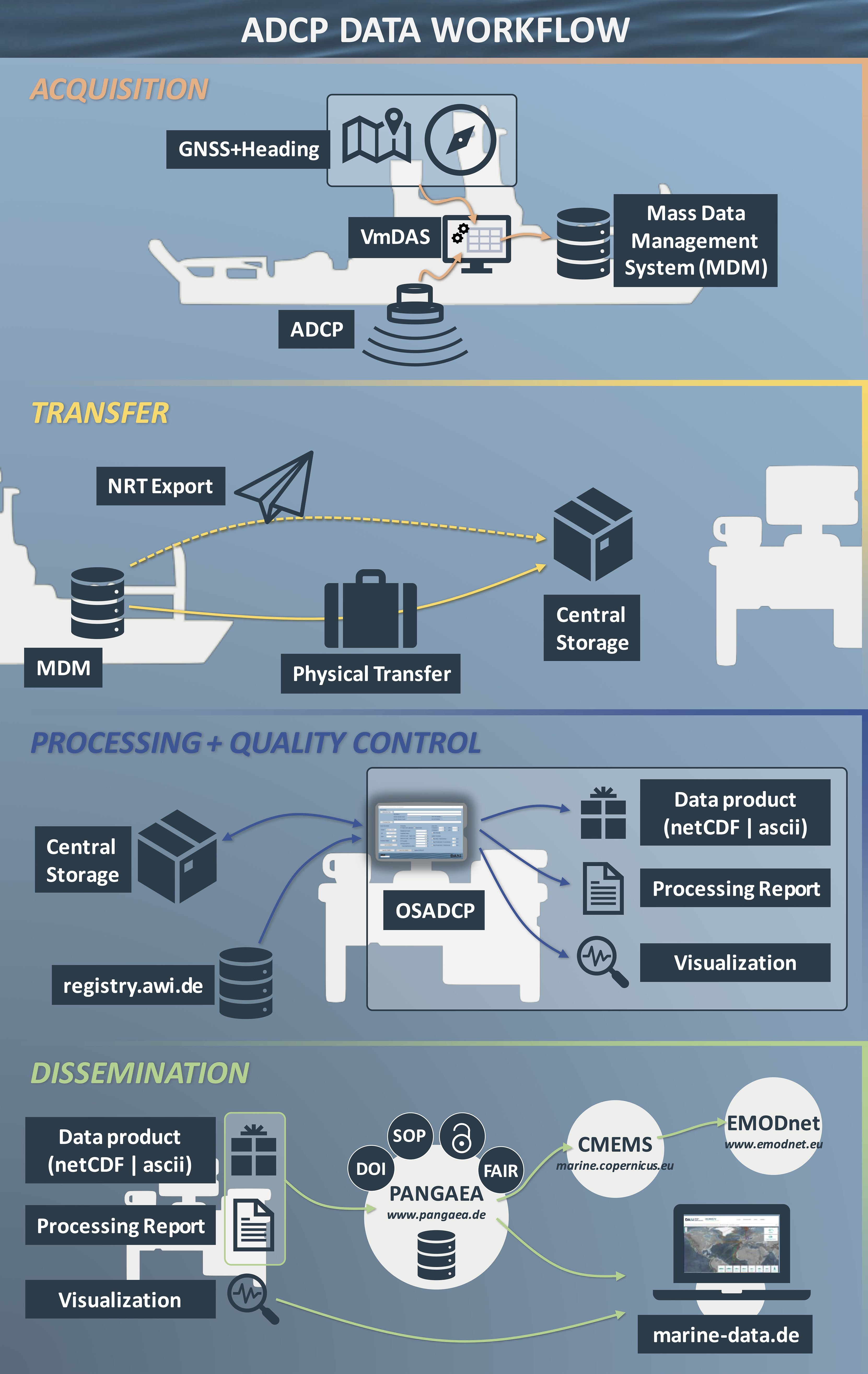
Figure 1. ADCP data workflow as implemented and established on the German research vessels R/V Maria S. Merian, R/V Meteor, and R/V Sonne (see Section 3 for details).
3.1 Data acquisition
The German marine research vessels R/V Maria S. Merian, R/V Meteor, and R/V Sonne are equipped with 75-kHz and 38-kHz Teledyne RDI Ocean Surveyor ADCPs for profiling the upper water column, up to 1200 m depth. High-quality, time-synchronous position and attitude data are provided by Kongsberg Seapath systems. Each VMADCP is controlled by a VMDAS instance installed on a dedicated sensor PC that bundles the VMADCP and navigation data streams. All raw data, that accumulates on the sensor PC is continuously backed up to the mass data management (MDM) system implemented in the IT infrastructure of each ship in the framework of the Underway Research Data project. The MDM system collects all recorded research data in a uniform, campaign-based manner and continuously mirrors it onto suitable transport hard drives.
In the workflow’s standard setting for routine underway deep-water profiling, VMDAS is configured to use narrowband single-ping recording with bottom-tracking disabled. Narrowband measurements are less sensitive to disturbances and noise or low abundances of scatterers in the water column. The profile parameters (number of cells/cell size/blanking distance) to set the sampling depths are chosen in the range of the recommended default values provided by the manufacturer for 75 kHz (100/8 m/8 m) and 38 kHz (50/32 m/16 m) systems.
VMDAS generates three, partly redundant raw data formats containing single-ping data in pd0 format, each representing a different status of internally applied coordinate transformation and data stream merging. ENR files contain velocities in beam coordinates but no external navigation data. ENS files additionally contain navigation data for each single ping. ENX files contain velocity data in earth coordinates and navigation data. Using ENR or ENS files to start post-processing, the required coordinate transformations (RD Instruments, 2010) are to be conducted by the user. In case of ENR files, the user also merges the ancillary data streams with the ADCP single-ping data. Starting with ENR or ENS files allows editing of single-ping data of individual beams and gives control to the user on how to perform the coordinate transformation (e.g., using a three-beam-solution if one beam is found malfunctioning). Starting with ENX files, the user needs to specify the sensors in the data acquisition setup that are to be considered as attitude data sources by the VMDAS internal coordinate transformation.
In addition to being inserted into the ENS and ENX files, the navigation data is logged in separate files. Binary format navigation data is collected in NMS files, while N[1,2,3]R files contain raw NMEA messages as configured in VMDAS. In the workflow’s standard setting, NMEA position data (GGA) and NMEA ship speed data (VTG) are collected in N1R files, and NMEA attitude (heading, pitch, roll) data (PRDID) are collected in N2R files. Additionally, PADCP messages with the ADCP ensemble number and a timestamp are contained in the N[1,2,3]R files. These can be used to align navigation data with the ADCP time series, if there was a problem with recording of the navigation data in the ENS or ENX files. VMDAS relies on the time settings of the recording PC when creating timestamps for pings, so it is advisable to keep the PC time synchronized with UTC time. Nonetheless, PADCP messages provided by VMDAS contain information on the difference between UTC and PC time, that can be used to correct ping times. VMDAS prioritizes inserting PADCP messages into the N[1,2,3]R files, which might occasionally corrupt other NMEA messages and complicates parsing during post-processing. Also, in the past, whole sections of navigation data could be corrupted by serial data overflows, but with modern IT infrastructure this is normally no longer a problem.
3.2 Data transfer
3.2.1 Near real-time
For system diagnostics and data quality checks, incoming VMADCP raw data is regularly sent ashore. A cronjob is watching the directory of VMADCP raw data on the MDM. Every hour, newly created ENX files (usually 10 MB in size) are identified, compressed and sent as a separate e-mail including meta information and a checksum. Ashore, data are received by the O2A ingest services for raw data (Koppe et al., 2015) hosted at Alfred-Wegener-Institute (AWI) in Bremerhaven, Germany and stored in the project’s central workspace.
3.2.2 Post-campaign transfer
In the destination port between two campaigns, the dedicated transport hard disks with a complete copy of the expedition data are removed from the MDM and sent to AWI as an insured shipment. In return, the ship receives empty hard drives for the next campaign. At AWI, the entire data set is checked for integrity and fed into the central workspace using the O2A ingest (Koppe et al., 2015) and is made accessible for delayed-mode processing and final quality control via the project’s central workspace.
3.3 Processing and quality control using OSADCP
The Python-based software OSADCP (Kopte et al., 2024) is developed both for the near-real-time monitoring and for the delayed-mode processing of the VMADCP raw data. OSADCP contains modules that include the essential processing steps (Figure 2) of coordinate transformation, position data verification, velocity data cleaning, bottom interference detection, ensemble averaging and water-track calibration. If configured in VMDAS, also bottom-track velocities can be used for the calculation of the velocity profiles. Customized add-on modules have been developed for the workflow presented here to automate for example the generation of data processing reports, data visualizations, or data format conversions for dissemination procedures.
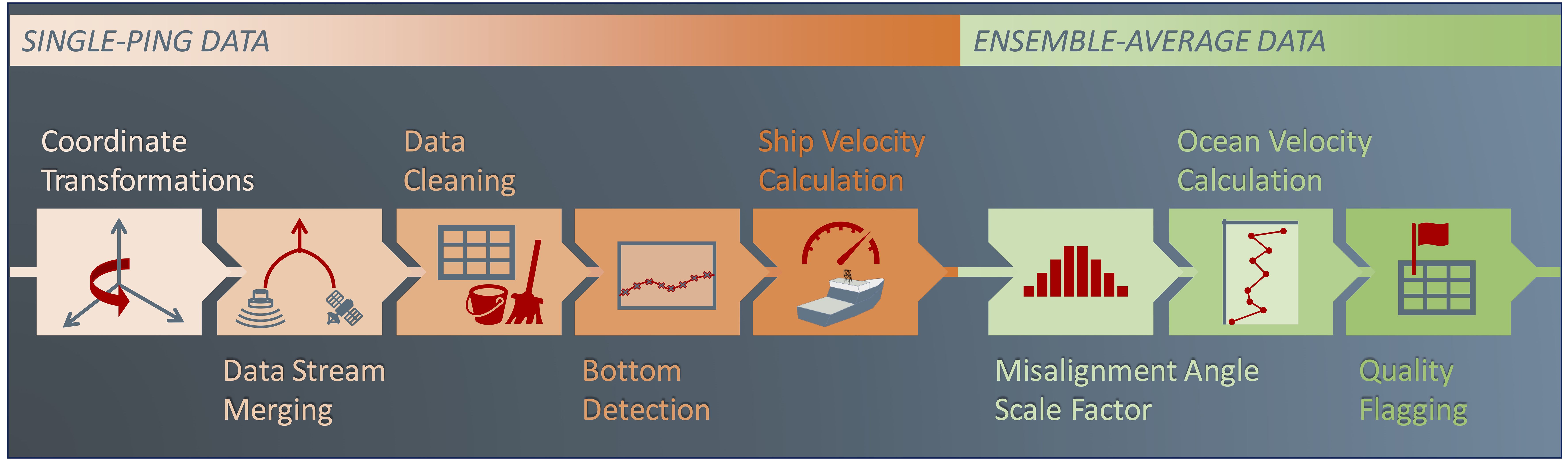
Figure 2. General processing chain for vessel-mounted ADCP data. Orange (green) colors represent steps carried out on the single-ping (ensemble-average) data (see Section 3.3 for details).
3.3.1 About OSADCP
OSADCP emerged from the MATLAB-based OSSI toolbox, which was developed over many years at GEOMAR, Helmholtz Centre for Ocean Research Kiel. As part of the DAM Underway Research Data project, it was redesigned and further developed to meet the requirements for standardized and, as far as possible, automated processing of VMADCP data from German research vessels. To facilitate access for the whole scientific community, OSADCP is written in Python. The software is designed to process VMADCP raw data acquired with Teledyne RDI’s data acquisition software VMDAS. A basic framework of the software is made available to the scientific community along with this article (see Appendix for instructions on the installation and setup). By default, OSADCP processes ENX files, which requires both high-quality and complete ADCP raw data and navigation data. From our experience, working with ENX files is generally preferred due to the simplicity of the handling. In the event that problems arise with either ADCP or navigation data, that require for example editing of beam-wise ADCP velocities or the manual merging of navigation data, OSADCP has add-on modules processing either ENR or ENS files that are not yet made publicly available.
The general procedure for working with OSADCP is shown in Figure 3. To illustrate key aspects of the processing we use an example data set from a 75 kHz Ocean Surveyor ADCP of the R/V Meteor campaign M189 (Dengler et al., 2023) that was acquired according to the workflow presented here.
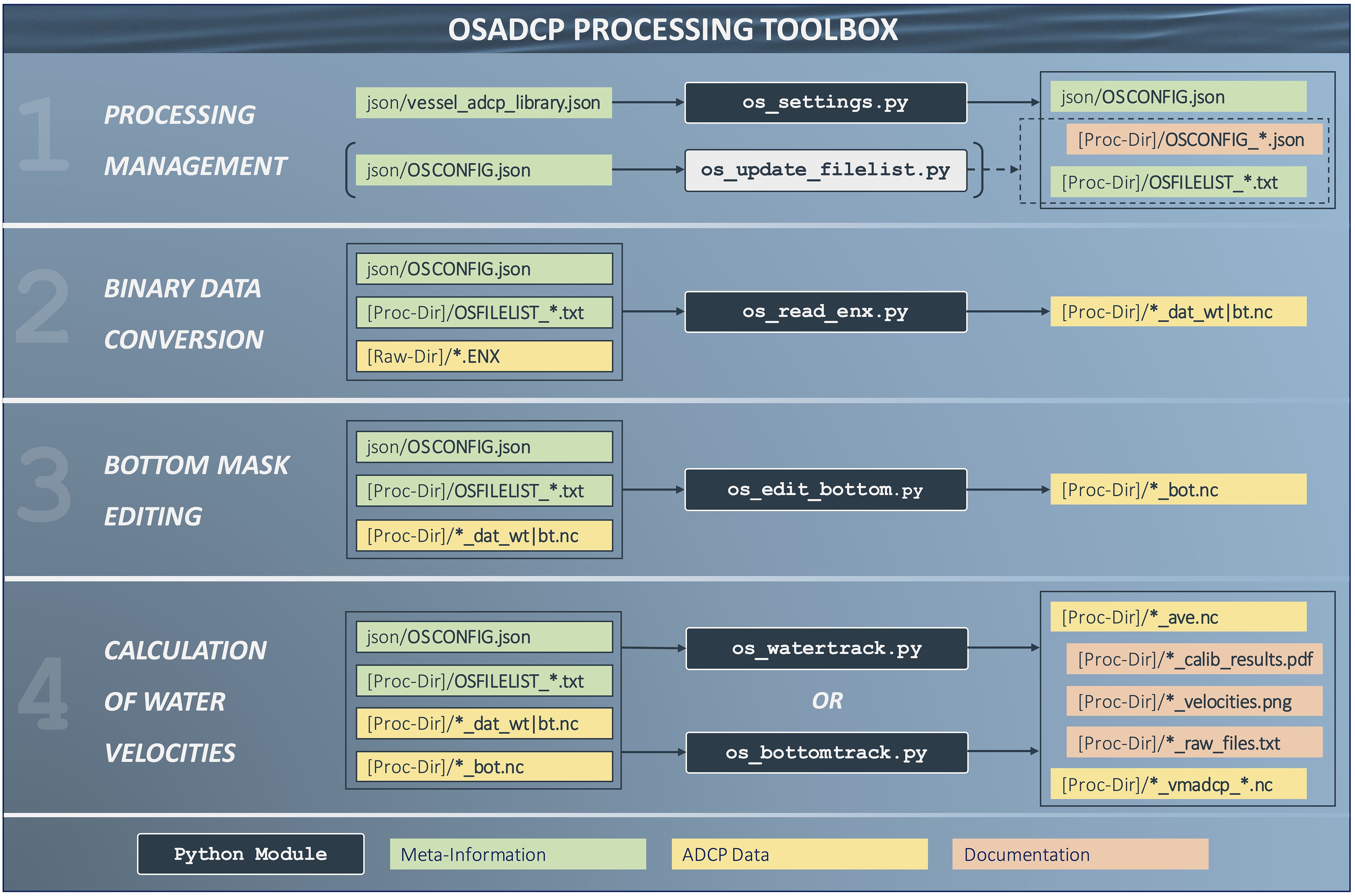
Figure 3. Workflow of the OSADCP processing toolbox. The main Python modules are depicted by dark blue boxes. Files storing major processing information are depicted in green boxes, ADCP data (binary pd0, intermediate netCDF files and final netCDF files) are represented by yellow boxes, while files documenting the processing are shown by orange boxes.
3.3.2 os_settings.py
A central point of the toolbox is the module os_settings.py, which runs a basic GUI (Figure 4). This GUI is used to create and modify a configuration json file for the processing. It makes use of the json dictionary json/vessel_adcp_library.json, where meta-information on vessel-specific ADCPs are stored (see Appendix).
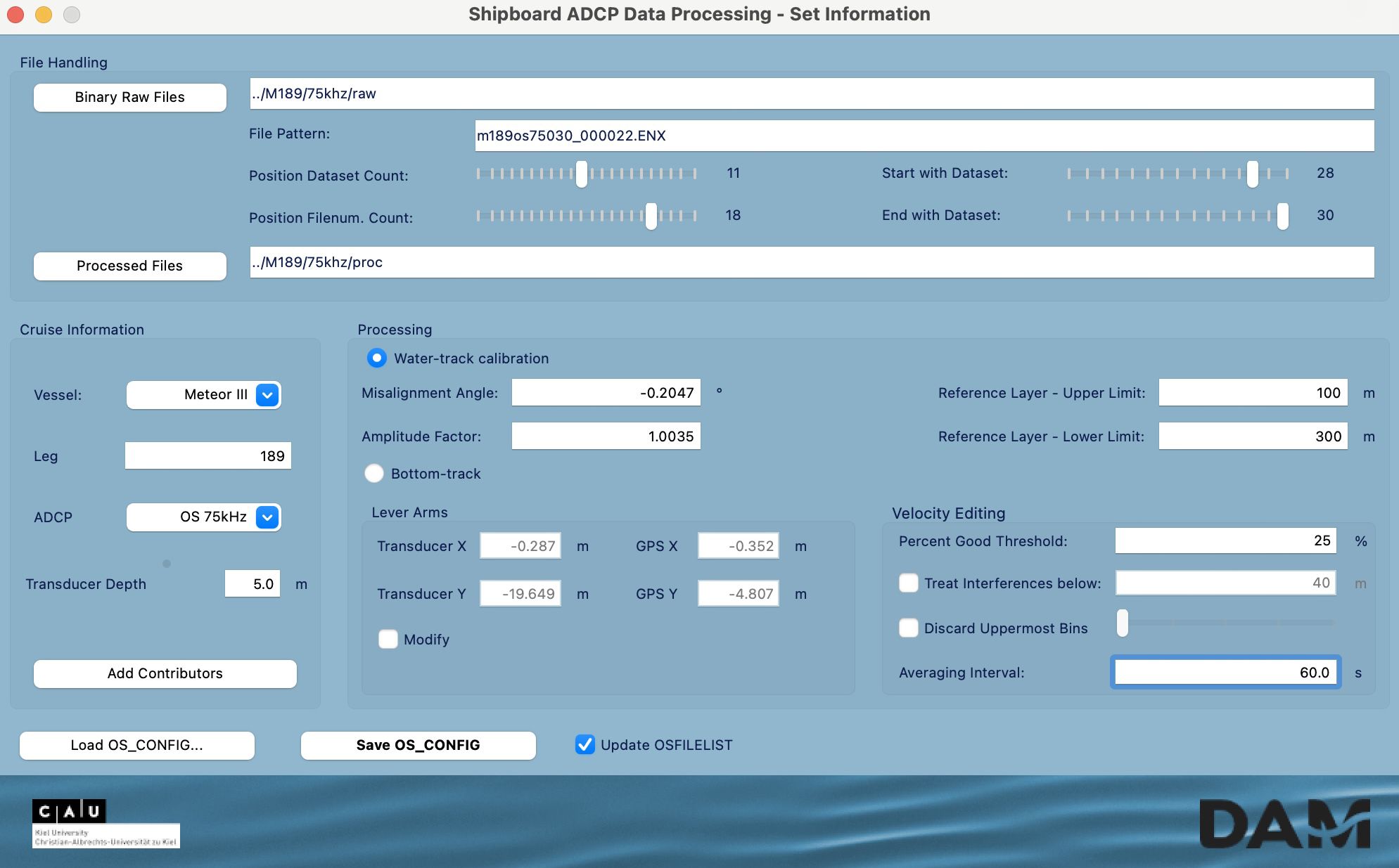
Figure 4. GUI controlling ADCP data processing in OSADCP. The GUI is executed via os_settings.py.
The configuration file is saved to json/OSCONFIG.json. A list of files to be processed is saved to the chosen processing directory, along with a copy of the configuration file for documentation purpose. Both the configuration file json/OSCONFIG.json and the list of files will be used by all other OSADCP processing modules (see Figure 3).
It is possible to load an existing configuration either from the working directory json/OSCONFIG.json or from any processing directory [proc_dir]/OSCONFIG_[adcp]_[vessel]_[leg].json, which is a common step when refining a data set or resuming work on an older dataset.
An alternative way is to manually edit the file json/OSCONFIG.json directly and then update the list of files and the configuration copy in the processing directory by executing the Python module os_update_filelist.py.
3.3.3 os_read_enx.py
The Python module os_read_enx.py is executed to loop over all files listed in [proc_dir]/OSFILELIST_*.txt and extract all VMADCP raw data and navigation data from the binary ENX files. For each binary raw data file, a corresponding netCDF file (Unidata, 2021) is saved to the processing directory, containing all data on the single-ping level (Figure 3). These files can be accessed for any user-specific editing on single-ping level not covered by the OSADCP standard treatment before continuing on the ensemble-average level.
A major task carried out by the module is the verification of the navigation data merged into the ENX files. Common problems include the occurrence of zero/zero positions when no real data is available due to problems of the navigation sensor and irregularities in the time allocation such as time stops, backward time jumps, time shifts etc. Affected pings are flagged accordingly and ignored in further processing. In the case of very poor navigation data, the manual insertion of external navigation data on single-ping level should be considered.
3.3.4 os_edit_bottom.py
An important aspect of the processing concerns the scanning for echo feedback from the ground, which introduces spurious velocities in the affected cell range. This task can be automated only to a limited extent since the echo intensity profile used for the identification is rarely unambiguous. It can be affected by acoustic interference in the water column or the occurrence of strong scattering layers, for example, that may lead to false bottom detection. Furthermore, near the sea bed velocities are potentially corrupted by sidelobe interference. Depending on the beam angle θ and the distance z to the ADCP transducer (ignoring pitch and roll tilts), velocities in the range above the bottom, the so-called shadow zone, are then contaminated by the sidelobe echo returning earlier to the transducer than the slanted main lobe. The detection and removal of spurious velocities beneath the shadow zone is a prerequisite for the subsequent water-track calibration, especially if the shadow zone depth overlaps with the reference layer chosen for the calibration (see os_watertrack.py below).
OSADCP provides the module os_edit_bottom.py that loops through all data files and lets the user decide whether a bottom signal is present and should be treated based on a visual inspection of the time series of the beam-averaged echo intensity (Figure 5, left panel). As the corresponding velocity bias in the shadow zone is most obvious in the along-track velocity while the ship is underway, it is shown as assisting information in the right panel of the interactive plot provided by os_edit_bottom.py. To visualize a potential velocity bias, the median along-track velocity is removed for each ping. Using the information provided in Figure 5, a line corresponding to the depth of bottom influence on the measured velocities is picked manually, adjusted as required and finally saved as a separate netCDF file with a *_bot.nc extension added to the file naming convention (Figure 2).

Figure 5. Interactive plot executed by os_edit_bottom.py, to pick the area affected by bottom interference. The left panel shows the average of the echo intensity measured by the four beams. The right panel shows the along-track velocity component with the median removed for each ping. The along-track component is displayed, which most prominently shows a potential velocity bias caused by bottom interference, in case of data collected underway. The echo intensity local maximum in the left panel corresponds to the bottom depth, while the transition towards high-biased along-track velocities in the right panel marks the depth of sidelobe interference by the bottom return echo. The red line is picked based on the information provided by the two panels. In subsequent processing steps, cells below the red line are ignored.
3.3.5 os_watertrack.py
The primary module of the software for deriving deep-water velocity profiles is called os_watertrack.py. It carries out important steps concerning the derivation of ship speed, the cleaning and averaging of single-ping data, and the estimation and application of the velocity calibration (Figure 2). For the treatment of single-ping data, the module loops over all data files created by os_read_enx.py during the binary data conversion (Figure 3). After averaging each data set separately, the module carries out the water-track calibration and calculation of water velocities based on the ensemble-averaged data of all data sets as specified by os_settings.py.
The ship speed is calculated via central differences based on the GNSS position data, ignoring only pings with questionable navigation data as flagged by os_read_enx.py. If the configuration file json/OSCONFIG.json contains lever arm information for the given setup of ADCP and GNSS sensor, the GNSS positions are corrected prior to the calculation of ship speed as follows:
with H being the ship’s heading, and and being the positions of the ADCP transducer and GNSS antenna relative to the ship’s center point along the minor and major axes of the ship, respectively (: starboard, : forward). This correction improves current velocities during ship maneuvers when the heading changes rapidly. In the example (Figure 6), the distance between ADCP and GNSS antenna was about 15 m. Single-ping data were combined into 1-minute ensembles and the approximately 3-hour excerpt contains three sections with abrupt changes of direction of the ship at around 06:30, 07:50, and 08:55 UTC (Figure 6A). Without lever arm correction, the derived direction of the ocean current profiles during these sections is notably different from the remaining time, where the ship’s heading is either constant or changes smoothly (Figure 6B). Geometric correction of the lever arms then improves the measured direction of ocean currents, here eliminating bands of erroneous current direction for the three sections (Figure 6C).

Figure 6. Effect of lever arm correction on the current direction. The data set was generated by a 75 kHz Ocean Surveyor ADCP during the M189 campaign of R/V Meteor (Dengler et al., 2023). (A) Ship heading on May 9, 2023. (B) Direction of the upper-ocean currents as 1-minute ensemble averages without lever arm correction applied, (C) same as (B), but with lever arm correction applied during post-processing. The distance between the ADCP transducer and the GNSS antenna was approximately 15 m along the main axis of the ship.
os_watertrack.py applies a number of automated cleaning criteria to the single-ping velocity data:
1. Error velocity: Large error velocities indicate a non-homogeneous flow field or large reflectors like fish, that cannot be assumed to move passively with the current. During the cleaning all cells are masked, where the derived cell error velocity exceeds twice the standard deviation of the error velocity.
2. Doubtful heading data: This criterion deals with unrealistic ship heading data by masking entire velocity profiles, where the ping-to-ping heading change exceeds 10°.
3. Doubtful current velocities: For this criterion, the single-ping current velocity is approximated by subtracting the ship velocity components from the measured velocities in the reference layer. Subsequently, entire velocity profiles are masked, either where the ping-to-ping change in either velocity component exceeds 2 m s-1, or where either velocity component exceeds 5 m s-1.
4. Acoustic interference: This is an optional cleaning criterion that can be enabled via os_settings.py, with additional control on the depth range considered for the cleaning (Figure 4). To detect spikes associated with acoustic interference, os_watertrack.py first constructs an echo intensity anomaly field by subtracting the median echo intensity profile from each echo intensity profile contained in the data file. Cells potentially affected by interference are then determined by identifying ping-to-ping differences that either exceed or fall below +0.7 or -0.7 of the total standard deviation of ping-to-ping differences, respectively. The candidate cells are then checked if they are of single-ping duration and whether the associated intensity spikes extend over several depth cells. All cells that are identified as being affected by acoustic interference are subsequently masked.
5. Bottom and sidelobe interference: To mask cells affected by the bottom return echo, os_watertrack.py reads the corresponding *_bot.nc files created by os_edit_bottom.py and applies the generated bottom interference mask to the single-ping velocity data.
Subsequently, single-ping data along the water column is averaged into so-called ensembles, with the velocities being vector-averaged. Using ensemble averages reduces the spread of single-ping current estimates, increasing the precision of the measurement. In os_watertrack.py the default average interval is 1 minute.
The water-track calibration implemented in os_watertrack.py addresses two different errors (Joyce, 1989; Firing and Hummon, 2010):
1. Misalignment error: A deviation of the transducer alignment with respect to the heading reference of the ship introduces a bias with its main effect being a spurious cross-track velocity component proportional to ship speed.
2. Scaling error: Small errors in the beam geometry or a non-zero trim of the transducer or ship can cause a systematic bias affecting mostly the along-track velocity component, proportional to ship speed.
The calibration aims at minimizing these errors by determining a misalignment angle correction and a scale factor correction , taking advantage of ship maneuvers involving speed changes. On research campaigns, such maneuvers primarily occur when approaching or leaving scientific stations, during which the ship is in parking position. Assuming that the true water velocities below the ship are constant during such maneuvers in a small area and over a short time interval, any measured variations in the absolute currents must result from the imperfect removal of the bias introduced by misalignment and scaling errors (Joyce, 1989; Fischer et al., 2003). To find possible calibration points, os_watertrack.py first calculates the time intervals, the distances travelled and the differences in ship speed between each ensemble and all other ensembles that are found within one hour. From this cloud of possible calibration points, all points with a distance covered of less than 5000 m and a minimum ship speed difference of 3 m s-1 are selected. In this way, different temporal and spatial scales are considered for the calibration. For all these points, the algorithm then minimizes the root-mean-square error between the corresponding ship velocities based on the GNSS position data and the velocities measured by the ADCP that are averaged over a certain depth range, the so-called reference layer. The upper and lower limits of this layer have to be defined via os_settings.py. The resulting noisy estimate of individual misalignment angles and scale factors is presented in a calibration plot (Figure 7). The individual estimates should cluster around some mean or median values, that represent the actual calibration values and . It is the user’s decision, whether the mean values should be applied directly to the data to refine the calibration. Alternatively, the processing can be continued with the previously entered values. In any case, desired values for the misalignment angle correction and scale factor correction can be entered via os_settings.py at any time. os_watertrack.py temporarily applies these values to the velocity data before carrying out the water-track calibration. Therefore, the clustering of optimized mean misalignment angles and the scale factors around 0 and 1 respectively (as shown in Figure 7) indicates a successful calibration.
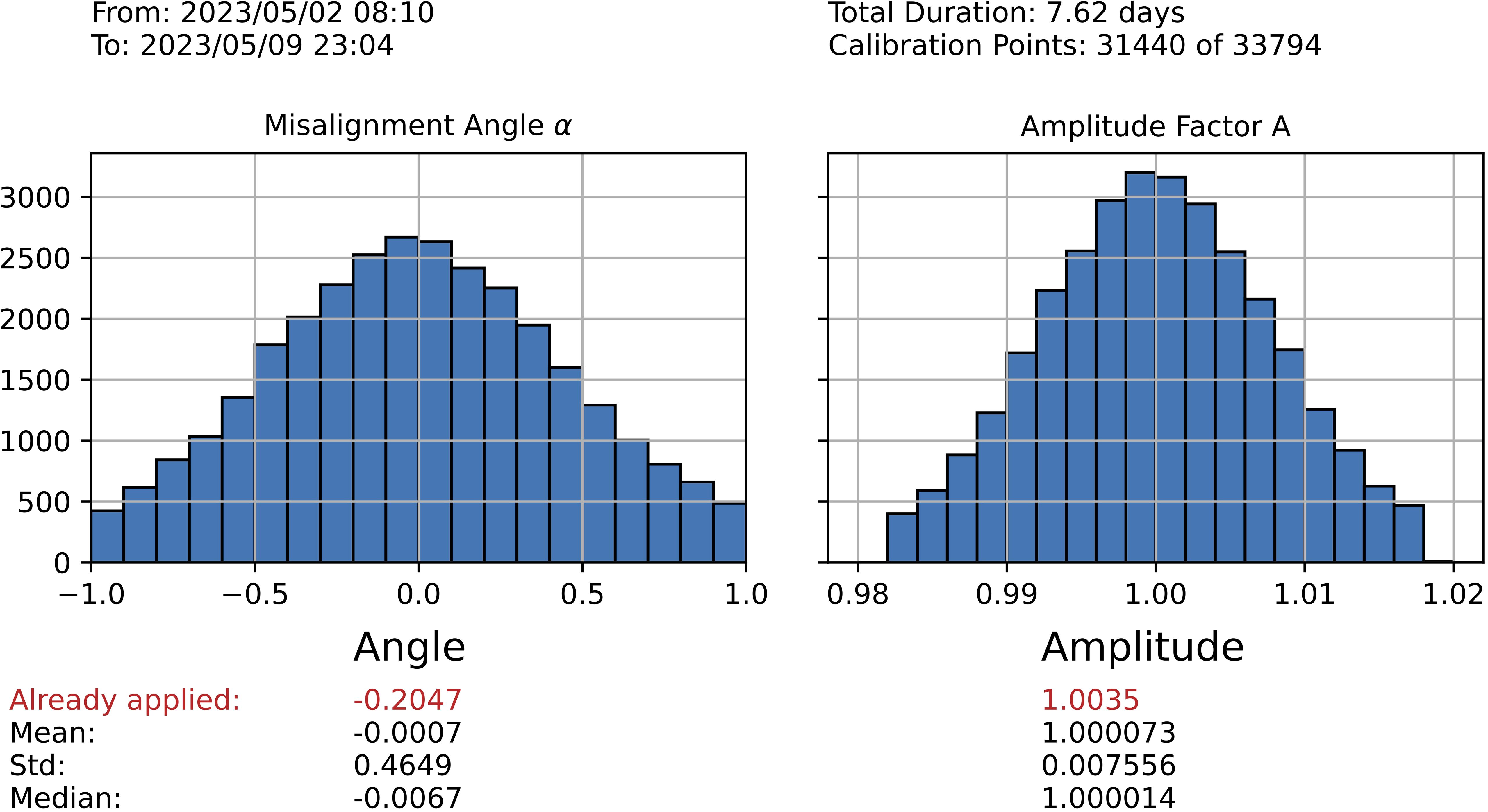
Figure 7. Results of OSADCP misalignment error and scale factor calibration for an exemplary data set: 75 kHz Ocean Surveyor ADCP during R/V Meteor cruise M189 (Dengler et al., 2023). Left histogram shows misalignment angle estimates clustering around zero, after a correction of -0.2047° was applied, right histogram shows corresponding results for the scale factor clustering around one, after a correction factor of 1.0035 was applied.
The final calibration values and are applied to the measured velocities . Taking into account the calculated ship velocities , the horizontal water velocities in east and north direction are then derived using the formula provided by Joyce, 1989:
3.3.6 os_bottomtrack.py
Even though bottom-track processing is not in the focus of this toolbox, a basic solution is provided by os_bottomtrack.py and can be used as alternative for os_watertrack.py. It contains a similar implementation for automated cleaning of single-ping including the application of the bottom mask to eliminate affected depth cells.
To use os_bottomtrack.py VMDAS needs to be configured to send bottom-track pings alternating to water-profile pings during data acquisition. The module then uses bottom-track velocities as ship speed over ground. At the single-ping level, the bottom-track velocities are directly subtracted from the water-profile velocities to obtain absolute current velocities. Because water-profile and bottom-track velocities share the instrument coordinate system, this operation does not introduce a cross-track velocity bias.
However, the module does not contain an implementation to determine the transducer orientation relative to the ship’s heading sensor to account for a potential transducer misalignment. Here, the misalignment results in an inaccurate estimate of the current’s direction rather than introducing a cross-track velocity bias, which is not as severe given a small misalignment angle.
3.3.7 Quality flagging
Both os_watertrack.py and os_bottomtrack.py contain an implementation for automated quality assessment. The flagging scheme follows the SeaDataNet vocabulary for measured qualifier flags (SeaDataNet, 2022).
The central criterion for the quality assessment is the evaluation of the ensemble percent-good value. The ensemble percent-good value is a measure of the number of valid measurements contained in an ensemble-mean. The ensemble percent-good threshold is defined via os_settings.py and saved in json/OSCONFIG.json. The default value of 25% is an empirical value to achieve a reasonable compromise between noise and range, where the expected error of cells with percent-good value of 25% is twice the expected error of cells with percent-good value of 100%. For applications where high accuracies are required it is advisable to select a higher percent-good threshold. Cells with an ensemble percent-good value below the defined threshold are flagged as “bad data”.
If a bias is detected in the top cells during post-processing, which is most likely associated with ringing or reverberation of the transducer or heavy sea conditions, affected cells can be flagged as “potentially bad data” for the whole deployment. Affected cells are selected via os_settings.py.
3.3.8 Meta data standards, documentation and archiving
The final data product of processed and quality-controlled VMADCP velocity measurements is created as netCDF file (Unidata, 2021).
Metadata standards follow Climate and Forecast conventions (CF-1.6, v19), OceanSites Manual-1.3, EGO glider user manual 1.3, and Attribute Convention for Data Discovery 1.3 (ACDD-1.3). Additionally, all relevant meta information about the deployment, VMADCP system, data acquisition and processing parameters are stored as global attributes (Figure 8). The standard name vocabulary to identify data variables is from CF-1.6, v19. Ensemble-mean time series of horizontal velocity profiles, and corresponding quality flags are stored as 2-D arrays, while the time, position and cell depth information are saved as 1-D vectors. The complete list of data variables contained by the netCDF file is shown by Figure 8.
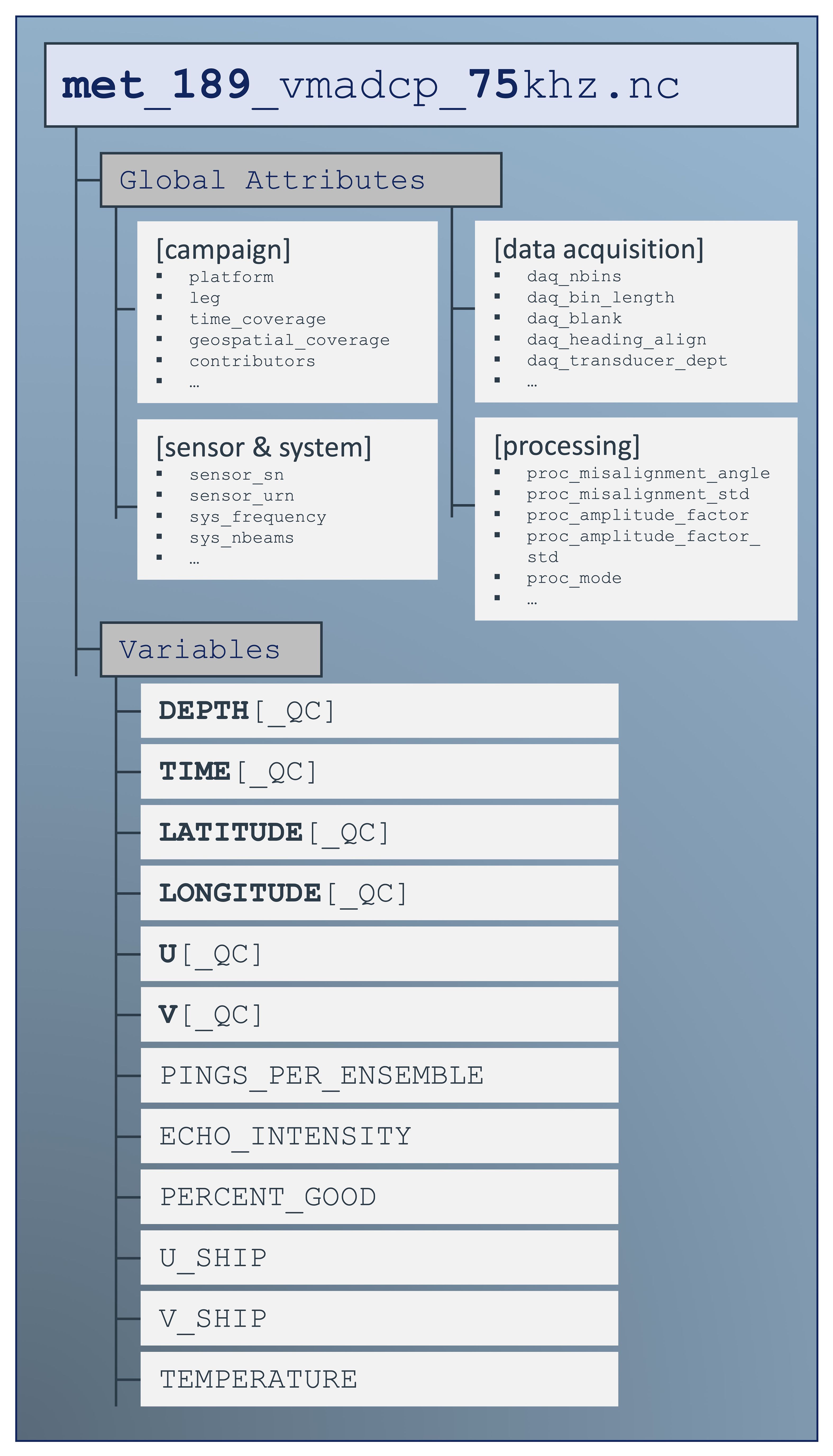
Figure 8. File structure of final netCDF VMADCP data file. Meta information are stored as netCDF global attributes and contain campaign-specific information, sensor and system data, data acquisition and processing parameters. The processed ensemble-mean data are stored as netCDF variables.
Using the meta information from the netCDF file, a processing report with the calibration diagram (Figure 7) and a map of the cruise track is automatically generated and saved in the processing directory of the corresponding data set. Also, a plot showing the resulting time series of the zonal and meridional velocity profiles is created for documentation purpose (Figure 9).
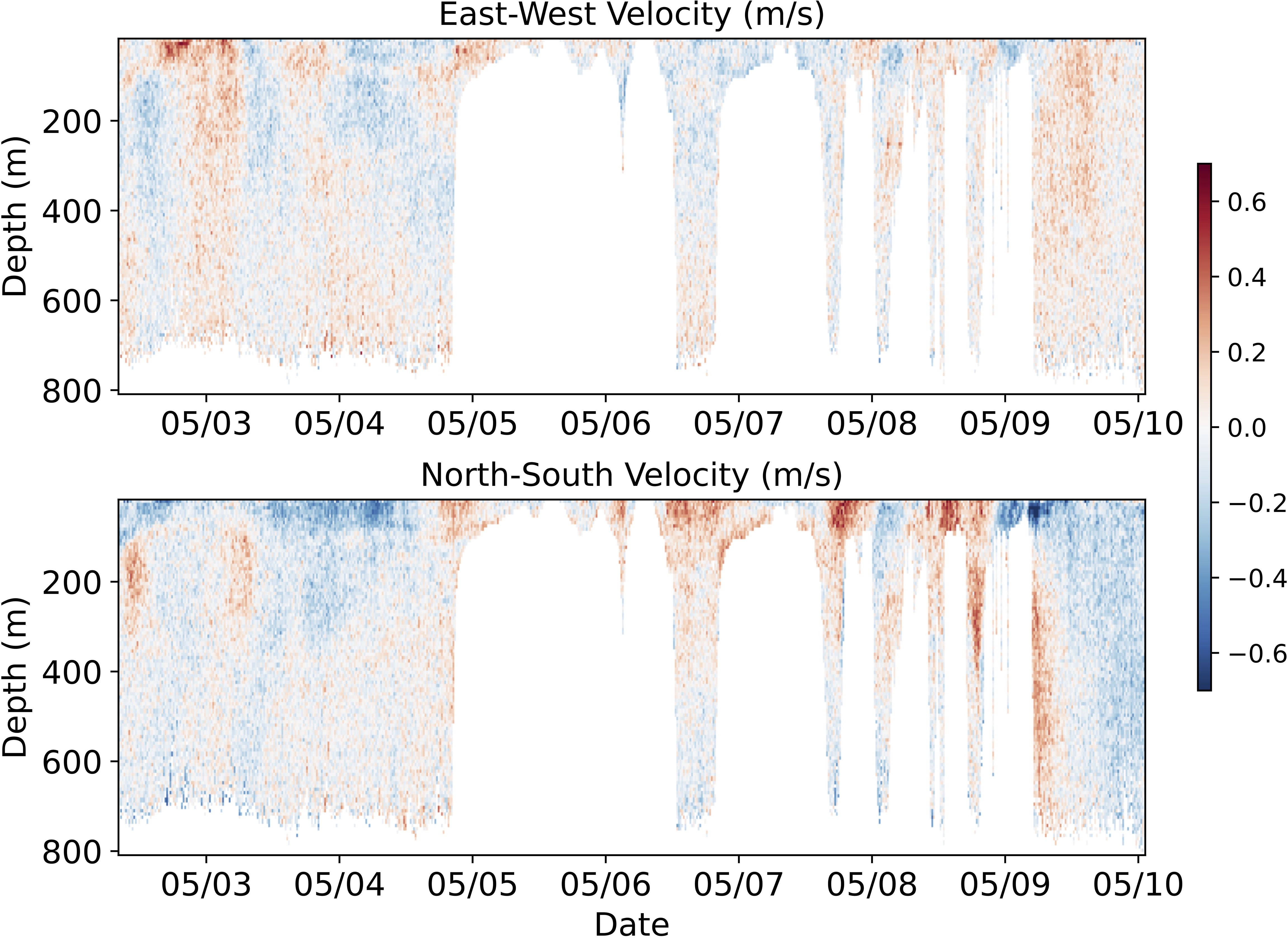
Figure 9. Final time series of zonal (top) and meridional (bottom) ocean currents after processing and calibration. White areas either correspond to missing data at the upper end of the profiling range, or to regions close to the sea bed, affected by bottom interference.
3.4 Data dissemination
3.4.1 PANGAEA
PANGAEA (https://www.pangaea.de) is the German node for delayed-mode data related to Earth system science (Felden et al., 2023), jointly operated by the Helmholtz Centre for Polar and Marine Research (AWI Bremerhaven) and the Center for Marine Environmental Sciences (MARUM) at the University of Bremen. The repository provides open access to curated and standardized data and includes a large range of data sets from different disciplines of Earth sciences.
PANGAEA is the target repository for the final ADCP data product. Prior to curation, an ASCII version of the netCDF file is created that is tailored for the integration in the PANGAEA database. Both the ASCII and the netCDF versions are submitted for each data set, as is the data processing report. As part of the data curation process, the data set is checked for completeness and assigned a DOI. The data set ensures open access and contains links to sensor-specific information, standard operating procedures and similar data sets.
3.4.2 marine-data.de
marine-data was developed and implemented in the framework of the DAM Underway Research Data project as the central access point for research data in German marine science. As a platform integrating several marine data repositories and services, marine-data is most closely linked to PANGAEA. Curated, high-quality datasets are provided by PANGAEA and promoted via marine-data as a coherent approach to improve their availability and interoperability.
At this stage, a visualization of the derived time series of eastward and northward current profiles similar to Figure 9 is prepared by a project-specific module of OSADCP, which is linked to the dataset DOI minted by PANGAEA. The visualization is provided by marine-data and may be used to assess the suitability of datasets for specific (research) purposes. marine-data in turn provides access for downloading the data sets from PANGAEA.
3.4.3 Link to European marine data repositories and services
To enhance their accessibility and interoperability, data sets acquired in the framework of the DAM Underway Research Data project are shared with other marine data repositories and data services through the DAM Data Broker. The Data Broker is an intermediary instance that prepares data sets provided by PANGAEA for seamless integration into other repositories or services. At this stage, data sets are forwarded primarily to Copernicus Marine Services (CMEMS, https://marine.copernicus.eu). CMEMS provides a wide range of oceanographic data sets, products and services, that are considered essential for monitoring and forecasting the state of the marine environment (see e.g. Schuckmann et al., 2021). From CMEMS, the data sets are further transferred to the European Marine Observations and Data Network (EMODnet, https://www.emodnet.eu, Martín Míguez et al., 2019) to the Physics portal. EMODnet Physics focusses on the compilation and dissemination of physical parameters related to the marine environment. Data is gathered from a network of European marine data providers and provided through a centralized portal. Both CMEMS and EMODnet Physics are components of the European marine infrastructure as they connect several data providers at European level, improving the accessibility and usability of marine data.
4 Summary and conclusions
This article introduces a workflow for VMADCP measurements implemented onboard German marine research vessels to provide high-quality and standardized ocean current data sets to the scientific community (Section 3). The workflow is designed for routine operation of VMADCP systems, which are integrated into the ship’s IT infrastructure, provided that navigation data streams are reliably available and that the installation parameters of all sensors are known. An important part of the workflow is the processing software OSADCP designed to work with binary raw pd0 data recorded by VMDAS from Teledyne RDI. The usage and implementations of OSADCP are described in detail in Section 3.3 to encourage the scientific community to apply the toolbox.
The workflow shows an example of a routinely applied data management strategy following FAIR data principles (Wilkinson et al., 2016). This type of data management covers the entire value chain from the sensor on the ship to the target repository PANGAEA, ready for scientific use. Data sets obtained in this way are published via the data portal marine-data.de. In addition, automated forwarding ensures a link to European data hubs providing in situ marine research data. At the time of writing, the inclusion of the data sets in the U.S. JASADCP archive is work in progress.
On research vessels used for deep-water oceanographic surveys, the ADCPs used are mainly Teledyne RDI Ocean Surveyors. In contrast, a variety of different ADCP systems are used in shallower waters and on smaller ships, in line with different requirements regarding the profiling range and the inferred physical parameters, e.g., turbulence and waves. These ADCPs are then configured according to the specific application and the specific deployment. With shallower waters, smaller ships, more heterogeneous, campaign-based setups and potentially more dynamic measurement environments, a whole range of challenges arise not only for data collection but also for post-processing (e.g., Muste et al., 2004; Vermeulen et al., 2014). These include, for example, the need for bottom-track processing in the presence of mobile, unconsolidated sea beds, to compensate for the inherent movements of smaller ships, increased positioning accuracy, and, in general, the adaptation of data processing to different setups. These challenges can only be met to a limited extent by one generic toolbox and are subject of future work.
The OSADCP toolbox as published along with this article, implements state-of-the-art processing for ADCP data acquired on larger ships and deeper water and assuming an appropriate setup and flawless data recording. The extended version of the toolbox includes additional functionalities for the integration into the workflow within the German marine research vessels. At present, the DAM Underway Research Data project extends the activities to smaller ships and different ADCP devices. Accordingly, the OSADCP toolbox is being expanded, too, implementing steps of post-processing as required in shallower water and in coastal environments.
Data availability statement
A publicly available dataset was used to illustrate the usage of the OSADCP software. This data can be found here: https://doi.pangaea.de/10.1594/PANGAEA.962916.
Author contributions
RK: Conceptualization, Data curation, Methodology, Software, Validation, Visualization, Writing – original draft, Writing – review & editing. MBec: Conceptualization, Project administration, Writing – original draft, Writing – review & editing, Funding acquisition. TF: Methodology, Software, Writing – review & editing, Validation, Writing – original draft. PB: Methodology, Software, Writing – review & editing. MBet: Writing – review & editing, Resources. GK: Writing – review & editing, Methodology, Software. CF: Resources, Software, Writing – review & editing. CW: Writing – review & editing. JK: Writing – review & editing. GW: Project administration, Writing – review & editing.
Funding
The author(s) declare financial support was received for the research, authorship, and/or publication of this article. This work is supported by KMS - Kiel Marine Science, the Center for Interdisciplinary Marine Science at Kiel University. MBec was funded by KMS and BAW (Federal Waterways Engineering and Research Institute, Hamburg, Germany). RK, MBet, and GW were funded through the Underway Research Data project of DAM, the German Marine Research Alliance. JK received funding by the European Union EuroGO-SHIP project (Grant agreement No 10194690).
Acknowledgments
We thank Jürgen Fischer, Christian Mertens, Marcus Dengler, Andreas Funk, Martin Vogt and Rena Czeschel for their contributions to the OSSI toolbox, the Matlab-based predecessor of OSADCP. We are specifically grateful for the support by the technical staff onboard the research vessels R/V Meteor, R/V Sonne, and, in particular, Emmerich Reize onboard R/V Maria S. Merian. We also like to acknowledge all our colleagues from the DAM Underway Research Data project for the excellent cooperation, in particular, Kathrin Riemann-Campe from the data publisher PANGAEA.
Conflict of interest
The authors declare that the research was conducted in the absence of any commercial or financial relationships that could be construed as a potential conflict of interest.
Publisher’s note
All claims expressed in this article are solely those of the authors and do not necessarily represent those of their affiliated organizations, or those of the publisher, the editors and the reviewers. Any product that may be evaluated in this article, or claim that may be made by its manufacturer, is not guaranteed or endorsed by the publisher.
References
Brandt P., Funk A., Tantet A., Johns W. E., Fischer J. (2014). The Equatorial Undercurrent in the central Atlantic and its relation to tropical Atlantic variability. Clim Dyn 43, 2985–2997. doi: 10.1007/s00382-014-2061-4
Carbotte S. M., O’Hara S., Stocks K., Clark P. D., Stolp L., Smith S. R., et al. (2022). Rolling Deck to Repository: Supporting the marine science community with data management services from academic research expeditions. Front. Mar. Sci. 9. doi: 10.3389/fmars.2022.1012756
Carroll S. R., Herczog E., Hudson M., Russell K., Stall S. (2021). Operationalizing the CARE and FAIR Principles for Indigenous data futures. Sci. Data 8, 108. doi: 10.1038/s41597-021-00892-0
Dengler M., Kopte R., Körner M., Imbol Koungue R. A. (2023). Shipboard ADCP current measurements (75 kHz) during RV METEOR cruise M189. doi: 10.1594/PANGAEA.962916
Felden J., Möller L., Schindler U., Huber R., Schumacher S., Koppe R., et al. (2023). PANGAEA - data publisher for earth & Environmental science. Sci. Data 10, 347. doi: 10.1038/s41597-023-02269-x
Firing E., Hummon J. (2010). “Ship-mounted acoustic Doppler current profilers,” in The GO-SHIP Repeat Manual: A Collection of Expert Reports and Guidelines. Eds. Hood E. M., Sabine C. L., Sloyan B. M. (IOCCP Report Number 14, ICPO Publication Series Number 134). Available online at: http://www.go-ship.org/HydroMan.html.
Firing E., Hummon J., Chereskin T. (2012). Improving the quality and accessibility of current profile measurements in the Southern Ocean. Oceanog 25, 164–165. doi: 10.5670/oceanog.2012.91
Fischer J., Brandt P., Dengler M., Müller M., Symonds D. (2003). Surveying the upper ocean with the ocean surveyor: A new phased array doppler current profiler. J. Atmos. Oceanic Technol. 20, 742–751. doi: 10.1175/1520-0426(2003)20%3C742:STUOWT%3E2.0.CO;2
Harris C. R., Millman K. J., van der Walt S. J., Gommers R., Virtanen P., Cournapeau D., et al. (2020). Array programming with numPy. Nature 585, 357–362. doi: 10.1038/s41586-020-2649-2
Hartl N., Wössner E., Sure-Vetter Y. (2021). Nationale forschungsdateninfrastruktur (NFDI). Informatik Spektrum 44, 370–373. doi: 10.1007/s00287-021-01392-6
Hummels R., Dengler M., Rath W., Foltz G. R., Schütte F., Fischer T., et al. (2020). Surface cooling caused by rare but intense near-inertial wave induced mixing in the tropical Atlantic. Nat. Commun. 11, 3829. doi: 10.1038/s41467-020-17601-x
Hummon J. M., Firing E., Gum J., Pinho U., Roc T., Vadnais D., et al. (2023). CODAS+UHDAS documentation. Geneva, Switzerland: Zenodo. doi: 10.5281/zenodo.8371259. https://currents.soest.hawaii.edu/docs/adcp_doc/index.html.
Hunter J. D. (2007). Matplotlib: A 2D graphics environment. Comput. Sci. Eng. 9, 90–95. doi: 10.1109/MCSE.2007.55
Johns W. E., Brandt P., Bourlès B., Tantet A., Papapostolou A., Houk A. (2014). Zonal structure and seasonal variability of the Atlantic Equatorial Undercurrent. Clim Dyn 43, 3047–3069. doi: 10.1007/s00382-014-2136-2
Johnson G. C., Sloyan B. M., Kessler W. S., McTaggart K. E. (2002). Direct measurements of upper ocean currents and water properties across the tropical Pacific during the 1990s. Prog. Oceanography 52, 31–61. doi: 10.1016/S0079-6611(02)00021-6
Joyce T. M. (1989). On in situ “Calibration” of shipboard ADCPs. J. Atmos. Oceanic Technol. 6, 169–172. doi: 10.1175/1520-0426(1989)006%3C0169:OISOSA%3E2.0.CO;2
King B. A., Firing E., Joyce T. (2001). “Chapter 3.1 Shipboard observations during WOCE,” in Ocean Circulation and Climate - Observing and Modelling the Global Ocean (San Diego, CA, USA: Elsevier), 99–122. doi: 10.1016/S0074-6142(01)80114-5
Koppe R., Gerchow P., Macario A., Haas A., Schäfer-Neth C., Pfeiffenberger H. (2015). O2A: A generic framework for enabling the flow of sensor observations to archives and publications. OCEANS 2015 - Genova, 1–6. doi: 10.1109/OCEANS-Genova.2015.7271657
Kopte R., Fischer T., Krahmann G., Brandt P., Faber C., Becker M. (2024). OSADCP Toolbox. (Kiel, Germany: GEOMAR). doi: 10.3289/SW_2_2024
L’Hégaret P., Schütte F., Speich S., Reverdin G., Baranowski D. B., Czeschel R., et al. (2023). Ocean cross-validated observations from R/Vs L’Atalante, Maria S. Merian, and Meteor and related platforms as part of the EUREC 4 A-OA/ATOMIC campaign. Earth Syst. Sci. Data 15, 1801–1830. doi: 10.5194/essd-15-1801-2023
Le Bot P., Kermabon C., Lherminier P., Gaillard F. (2011). CASCADE V6.1: Logiciel de validation et de visualisation des mesures ADCP de coque. Retrieved from https://archimer.ifremer.fr/doc/00342/45285/.
Lindstrom E., Gunn J., Fischer A., McCurdy A., Glover L. K., Members T. T. (2012). A Framework for Ocean Observing. (Paris, France: UNESCO). doi: 10.5270/OceanObs09-FOO
Martín Míguez B., Novellino A., Vinci M., Claus S., Calewaert J.-B., Vallius H., et al. (2019). The european marine observation and data network (EMODnet): visions and roles of the gateway to marine data in europe. Front. Mar. Sci. 6. doi: 10.3389/fmars.2019.00313
Menkes C. E., Kennan S. C., Flament P., Dandonneau Y., Masson S., Biessy B., et al. (2002). A whirling ecosystem in the equatorial Atlantic. Geophysical Res. Lett. 29:48-1 - 48-4. doi: 10.1029/2001GL014576
Muste M., Yu K., Spasojevic M. (2004). Practical aspects of ADCP data use for quantification of mean river flow characteristics; Part I: moving-vessel measurements. Flow Measurement Instrumentation 15, 1–16. doi: 10.1016/j.flowmeasinst.2003.09.001
Pinkel R., Smith J. A. (1992). Repeat-sequence coding for improved precision of doppler sonar and sodar. J. Atmos. Oceanic Technol. 9, 149–163. doi: 10.1175/1520-0426(1992)009%3C0149:RSCFIP%3E2.0.CO;2
RD Instruments. (2010). ADCP coordinate transformation: formulas and calculations. San Diego, CA, USA: RD Instruments.
RD Instruments. (2011). Acoustic Doppler Current Profilers Principles of Operation: A Practical Primer. San Diego, CA, USA: RD Instruments.
Riverbank Computing Limited. PyQt5 (a set of Python bindings for v5 of the Qt application framework from The Qt Company); software available at: https://www.riverbankcomputing.com/software/pyqt/
Schuckmann K., Le Traon P.-Y., Smith N., Pascual A., Djavidnia S., Gattuso J.-P., et al. (2021). Copernicus marine service ocean state report, issue 5. J. Operation. Oceanogr. 14, 1–185. doi: 10.1080/1755876X.2021.1946240
SeaDataNet (2022). SeaDataNet Measured Qualifier Flags. Available online at: https://vocab.nerc.ac.uk/collection/L20/current/ (Accessed November 09, 2023).
Shcherbina A. Y., Sundermeyer M. A., Kunze E., D’Asaro E., Badin G., Birch D., et al. (2015). The latMix summer campaign: submesoscale stirring in the upper ocean. Bull. Am. Meteorological Soc. 96, 1257–1279. doi: 10.1175/BAMS-D-14-00015.1
Sprintall J., Chereskin T., Sweeney C. (2012). High-resolution underway upper ocean and surface atmospheric observations in drake passage: synergistic measurements for climate science. Oceanog. 25, 70–81. doi: 10.5670/oceanog.2012.77
Unidata (2021). Network Common Data Format (netCDF) version 1.5.8 [software]. Boulder, CO: UCAR/Unidata Program Center. doi: 10.5065/D6H70CW6
Vermeulen B., Sassi M. G., Hoitink A. J. F. (2014). Improved flow velocity estimates from moving-boat ADCP measurements. Water Resour. Res. 50, 4186–4196. doi: 10.1002/2013WR015152
Virtanen P., Gommers R., Oliphant T. E., Haberland M., Reddy T., Cournapeau D., et al. (2020). SciPy 1.0: fundamental algorithms for scientific computing in Python. Nat. Methods 17, 261–272. doi: 10.1038/s41592-019-0686-2
Wilkinson M. D., Dumontier M., Aalbersberg I. J. J., Appleton G., Axton M., Baak A., et al. (2016). The FAIR Guiding Principles for scientific data management and stewardship. Sci. Data 3, 160018. doi: 10.1038/sdata.2016.18
Appendix - OSADCP installation and setup
OSADCP requires a working and reasonably current Python3 installation. Depending on the operating system, an installation of QT5 might be required. Although it is perfectly possible to install OSADCP within the system’s main Python installation, some kind of isolation, such as a virtual environment, is recommended. OSADCP is built primarily with the following open-source packages: numpy, scipy, PyQt5, matplotlib, netCDF4 (in order: Harris et al., 2020; Virtanen et al., 2020, Riverbank Computing, Hunter, 2007; Unidata, 2021).
The OSADCP toolbox is published via a Git repository at https://git.geomar.de/dam/osadcp_toolbox. It can be downloaded as zip archive and extracted locally. Alternatively, if the user has Git installed, the following command can be used to download the toolbox: git clone https://git.geomar.de/dam/osadcp_toolbox.git.
Subsequently, OSADCP’s dependencies as specified in the requirement file need to be installed via pip install -r requirements.txt. Please refer to the git repository for the latest version of the toolbox and for updated installation instructions and user manuals.
After setting up the toolbox, meta-information on ADCPs and vessels, such as serial numbers, lever arms etc., can be added to the json-dictionary json/vessel_adcp_library.json. This dictionary manages ADCP and vessel-specific metadata centrally and is used by the processing management module (Section 3.3) for efficient allocation and forwarding.
Keywords: ADCP, underway data, FAIR data, python, ocean currents
Citation: Kopte R, Becker M, Fischer T, Brandt P, Krahmann G, Betz M, Faber C, Winter C, Karstensen J and Wiemer G (2024) FAIR ADCP data with OSADCP: a workflow to process ocean current data from vessel-mounted ADCPs. Front. Mar. Sci. 11:1425086. doi: 10.3389/fmars.2024.1425086
Received: 29 April 2024; Accepted: 02 August 2024;
Published: 26 August 2024.
Edited by:
Sarah T. Gille, University of California, San Diego, United StatesReviewed by:
Eric Firing, University of Hawaii at Manoa, United StatesAntonio Novellino, ETT SpA, Italy
Copyright © 2024 Kopte, Becker, Fischer, Brandt, Krahmann, Betz, Faber, Winter, Karstensen and Wiemer. This is an open-access article distributed under the terms of the Creative Commons Attribution License (CC BY). The use, distribution or reproduction in other forums is permitted, provided the original author(s) and the copyright owner(s) are credited and that the original publication in this journal is cited, in accordance with accepted academic practice. No use, distribution or reproduction is permitted which does not comply with these terms.
*Correspondence: Robert Kopte, cm9iZXJ0LmtvcHRlQGlmZy51bmkta2llbC5kZQ==