Tide-surge interactions in Northern South China Sea: a comparative study of Barijat and Mangkhut (2018)

In this study, the storm surge processes and characteristics of Tide-Surge Interactions (TSI) induced by the sequential tropical cyclones (TCs) BARIJAT and MANGKHUT (2018) in the Northern South China Sea (NSCS) are investigated using the numerical model. By comparing the impacts of the two TCs, we find that storm surges are significantly influenced by multiple factors. Notably, bays situated on the western side of the cyclone’s landfall point exhibit a double peak pattern in storm surge. In addition, TSI exhibits a pronounced impact across bays affected by the two TCs, with amplitude fluctuations ranging from -0.3 to 0.3 meters and contributing approximately -5% to -20% to the peaks of storm surge. Comparative analysis of TSI variations reveals that tides act as the primary determinant, significantly influencing both the magnitude and period of TSI. Dynamic analysis further highlights that variations in TSI are dominated by barotropic pressure gradient and bottom friction stress. Moreover, TSI affects the frequency of storm surges, introducing high-frequency tidal signals to storm surges and reducing the frequency of storm surges.

1 Introduction

Storm surges, a catastrophic sea level rise induced by hurricanes or typhoons through abrupt meteorological changes, have historically posed significant threats to coastal regions, leading to both substantial economic losses and human casualties. When combined with astronomical tides, these surges can result in extreme water levels, exacerbating their impact on coastal populations and infrastructures (Choi et al., 2003). Over the past two centuries, storm surges have been responsible for approximately 2.6 million fatalities worldwide, with an annual average of 13,000 lives lost directly or indirectly due to these disasters (Nicholls, 2003). Super typhoons or hurricanes have inflicted substantial financial damages on coastal populations, with the most severe impacts observed in the United States, southeastern China, Japan, and the Philippines. Notably, hurricanes such as Katrina (2005), Sandy (2012), Maria (2017), Harvey (2017), and Lan (2022) have collectively resulted in an estimated economic loss of approximately $677.1 billion in the United States alone, as reported by NOAA (2024). A considerable portion of these losses can be attributed to storm surge disasters, highlighting their devastating financial impact (Genovese and Green, 2015).

The intensity of disasters brought by storm surges is closely related to the magnitude and duration of storm surges. Previous research has demonstrated that storm surges are influenced by multiple factors, including the intensity of the typhoon, topographic effects, the point of landfall, the speed of the typhoon’s movement, and the radius of its impact, presenting significant challenges to the forecasting and early warning of storm surge disasters (Weisberg and Zheng, 2006; Irish et al., 2008; Rego and Li, 2009; Sebastian et al., 2014). Wu et al. (2018) highlights that waves also significantly influence storm surge heights and inundation distances, with their effects varying substantially based on storm characteristics such as intensity, size, translation speed, and incident angle, underscoring the need for nuanced modeling of storm surge dynamics under different storm conditions. In the detailed modeling of extreme nearshore water levels, Tide-Surge Interactions (TSI) plays a crucial role in modulating coastal water levels (Zhuge et al., 2024). However, in the prediction and early warning of storm surges, the influence of TSI cannot be overlooked, exerting a pronounced impact on water levels in coastal regions with complex topographies. For instance, Yuk et al. (2015) used a coupled tide-surge model to reproduce storm surges more accurately than an uncoupled model. In the southern Yellow Sea, TSI reached a maximum of 1.09 meters and an average of 0.97 meters (Zhang et al., 2019). A case study in Tieshan Bay indicated that the storm surge was modified by TSI, being enhanced or suppressed by up to 0.94 meters (Yang et al., 2019). This highlights the need for advanced modeling and analytical approaches to accurately assess and predict the impacts of storm surges and the mechanisms of TSI, considering the intricate interplay of meteorological and oceanographic factors.

The intricate mechanisms underlying TSI are essential to understanding the dynamics of coastal storm surges, particularly in estuarine environments where the interplay between tides and surges can significantly influence surge heights. Pioneering research by Proudman and Pearson (1957) introduced analytical solutions for the advancement of tides and storm surges within uniformly shaped estuaries, uncovering that interactions between tides and surges led to diminished storm surge heights near high tide compared to those near low tide for propagating waves. Rossiter and Lennon (1968) identified mutual phase shifting as a fundamental aspect of tide-surge dynamics, illustrating how negative surges delay tidal peaks, whereas positive surges accelerate them. Further investigations by Horsburgh and Wilson (2007) revealed a tendency for reduced surge formation around high tides, suggesting a lower probability of surge peaks coinciding with high tide during significant tidal amplitudes.

The complexity of TSI is broadly understood to encompass three nonlinear physical processes: horizontal and vertical advection effects, quadratic bottom friction influences, and variations due to total water depth, affecting both momentum and continuity equations (Tang et al., 1996; Bernier and Thompson, 2007; Zhang et al., 2010, 2017). Further elaboration on this dynamic interaction using a simplified analytical model to simulate the characteristics of TSI in the North Sea, Northumberland Strait, and Río de la Plata revealed that the quadratic bottom frictional term plays a significant role in creating interaction effects (Prandle and Wolf, 1978; Bernier and Thompson, 2007; Dinápoli et al., 2020). Additionally, topographic coastal trapping, the funneling effect, and the angle between the storm track and the coastline also play essential roles in storm surge simulation (As-Salek, 1998; As-Salek and Yasuda, 2001).

Moreover, increasing attention is being focused on sequential TCs. Climate projections under the SSP5 8.5 scenario indicate a significant rise in the frequency of sequential TC landfalls during the 21st century, with the chance of a location experiencing a less-than-10-day break between two TC impacts being doubled for most regions (Xi and Lin, 2021). The proportion of storm surge disasters caused by sequential typhoons is also markedly increasing (Xi et al., 2023). However, the aforementioned studies are based on synthetic typhoons under future scenarios, and comparative research on real sequential TCs remains scarce. The typhoons Barijat and Mangkhut that struck the Northern South China Sea (NSCS) in 2018 provide a pertinent case study; they made landfall consecutively within five days, with Mangkhut, a super typhoon, causing substantial economic losses and casualties upon its landfall in the NSCS. Mangkhut (2018) was the strongest typhoon to strike the NSCS since Megi in 2010 and the strongest to make landfall anywhere in the Philippines since Meranti in 2016. Mangkhut was also the strongest typhoon to affect Hong Kong since Ellen in 1983. Thus, research on such actual instances of sequential TCs holds significant importance.

Sequential typhoons landing with intervals shorter than the recovery times of coastal communities and ecosystems pose significant risks. For instance, typhoons can disrupt power supply, leading to widespread outages (Huang and Wang, 2024). They can also paralyze urban transportation systems and cause extensive cessation of ship operations (Hu and Ho, 2015). Moreover, the debris from typhoon-induced damage to buildings requires substantial cleanup time and renders structures more vulnerable to subsequent storms (Lin et al., 2010). Typhoons affect coastal ecosystems as well; for example, storm surges can lead to estuarine saltwater intrusion, with successive intrusions having significant ecological impacts (Gao et al., 2024). Regarding Typhoons Barijat and Mangkhut (2018), news reports indicated that Barijat caused power outages for 30,000 households in Guangdong, followed by Mangkhut, which resulted in outages for 1.7 million households. The short interval between these sequential typhoons might have delayed electrical repairs, affecting the restoration of power supply. Additionally, both Barijat and Mangkhut brought extensive continuous rainfall, potentially causing significant economic losses.

Previous research has primarily concentrated on assessing TSI during specific tropical cyclone occurrences, lacking a comparative cross-sectional analysis of TSI during sequential TC events. Furthermore, a definitive consensus on whether storm surges or tidal influences predominantly contribute to TSI is yet to be established. Studies examining the dynamic mechanisms underlying TSI are also relatively scarce. Under varying intensities of typhoons, the impact of TSI on storm surges remains underexplored in current research. Consequently, this study aims to comprehensively investigate the storm surge and TSI impacted by TCs of varying intensities. The expected findings aim to offer valuable insights for coastal planning and management, thereby contributing to the sustainable development of coastal communities.

2 Materials and methods

2.1 Mangkhut and Barijat in 2018

Typhoon Mangkhut (2018), the 22nd typhoon of 2018, formed on September 7th at 08:00 (UTC+8, as below) on the western Pacific Ocean surface. It began moving westward and intensified into a violent typhoon, reaching maximum central wind speeds of 65 m/s. On September 15th at 03:00, it made landfall in the northern Philippines, with its central wind speed decreasing to 48 m/s post-landfall. Continuing northwestward, the typhoon entered the South China Sea. Subsequently, it made its second landfall on September 16th at 17:00 in Taishan City, Guangdong Province, China, with a recorded maximum wind speed of 43 m/s, as shown in Figures 1E–H. It then traversed Guangdong Province and entered Guangxi Province, with rapidly diminishing wind speed. Mangkhut brought heavy rainfall, strong winds, and severe storm surge disasters to the Guangdong coastal region. Numerous houses collapsed, trees were uprooted, and issues such as power outages and transportation disruptions were widespread. The maximum observed storm tide was recorded at the Sanzao station in Guangdong Province, reaching 3.39 meters, with over ten stations reporting surges exceeding 1 meter. According to China’s Ocean Disaster Monitoring and Early Warning Technology Laboratory (CODMEWTL, 2019), Mangkhut caused economic losses estimated at 19.37 billion yuan, resulting in 129 fatalities.

Figure 1

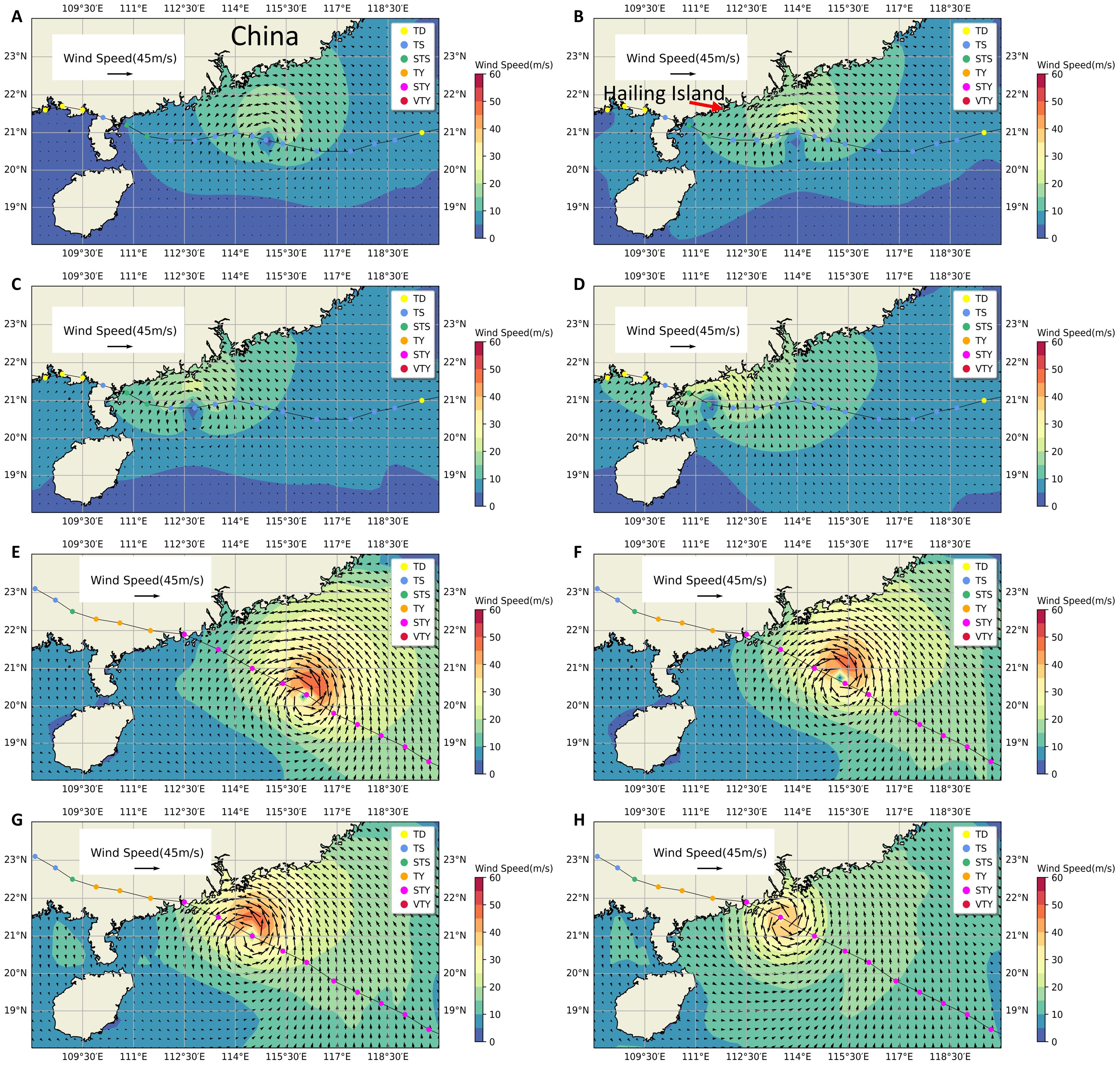
Figure 1. The spatial distribution of the movement track and wind speed of TCs Barijat and Typhoon Mangkhut (2018) in the NSCS. (A–D) respectively represent the wind field of Barijat from 03:00 on September 12th to 21:00 on September 12th, with a map generated every six hours; (E–H) respectively represent the wind field of Mangkhut from 21:00 on September 15th to 06:00 on September 16th, with a map generated every three hours.

Tropical cyclone Barijat, a severe tropical storm and the 23rd typhoon of 2018, was initially categorized as a tropical depression by the China Meteorological Administration in the Luzon Strait on September 10th at 08:00. It initially affected the NSCS, causing notable storm surges. By September 11th, Barijat was classified as a tropical storm, and it progressed to a severe tropical storm by approximately 05:00 on September 13th. Around 08:30 on the same day, the typhoon made landfall along the coast of Zhanjiang City, Guangdong Province. At the time of landfall, the maximum near-center wind force reached 25 m/s, as shown in Figures 1A–D.

Mangkhut and Barijat (2018), which strongly affected the water level in the coastal region of NSCS, exhibited differing intensities and velocities. Although Barijat did not attain the same wind speed as Mangkhut, it also led to significant storm surges. The short interval between these two TCs resulted in consecutive impacts along the Guangdong coastal area. Therefore, we conducted a comparative analysis of the storm surge processes and characteristics in the NSCS caused by these two TCs, as well as the variations in TSI triggered by both events.

2.2 The numerical model

In this study, the 2004 version of the Princeton Ocean Model (POM) was utilized to investigate the storm surge characteristics and TSI mechanisms in the NSCS during Barijat and Mangkhut (2018). POM is a three-dimensional, fully nonlinear ocean model based on primitive equations (Mellor and Yamada, 1982; Mellor, 2004). It has undergone multiple revisions and enhancements, evolving into a reliable model for estuarine and nearshore ocean dynamics. As a three-dimensional primitive equation model, POM enables a more accurate representation of storm surge processes and the mechanisms of TSI.

The model domain covers the region within 16-25°N and 105-121°E, encompassing the entire NSCS area. The horizontal grid resolution is set at one arcminute, approximately 1.86 kilometers, resulting in a grid containing 4,665,699 elements and 519,901 nodes. For the vertical grid, POM uses a sigma coordinate system, and we divided the vertical grid into five layers. The model employs tidal boundaries derived from the global tidal model TPXO (Egbert and Erofeeva, 2002), extracting eight tidal constituents (M2, S2, N2, K2, K1, O1, P1, Q1) to generate tidal boundary water levels. Both tidal boundaries and atmospheric forcing drive the model. Initialization occurred from a cold start on September 1, 2018, with the model running for 18 days, including a spin-up period of two to three days.

The bathymetric and depth data utilized in this study are sourced from the GEBCO Bathymetric Compilation Group, 2019 version, with a 15 arc-second resolution (Becker et al., 2009; GEBCO Bathymetric Compilation Group, 2019; Sandwell et al., 2014; Tozer et al., 2019). However, the GEBCO dataset presents inaccuracies in the topography of the Pearl River Estuary, where islands are not delineated, and inaccuracies exist in water depth measurements. To enhance the precision of simulation outcomes, we have refined the bathymetric chart of the Pearl River Estuary by incorporating information from nautical charts.

The study area of the model includes the Pearl River Estuary region. The Pearl River, the third-largest river in China, flows into the NSCS through eight outlets, with a significant mean summer flow rate. The Pearl River profoundly impacts the physical and biological characteristics of the NSCS region (Wong et al., 2003; Liao et al., 2020). Additionally, previous researchers collectively indicate that in high-discharge river mouths such as the Mississippi River, Pearl River, and Yangtze River, the river discharge significantly influences the simulation of water levels at river estuaries and should not be disregarded (Kerr et al., 2013; Duan et al., 2015; Wang et al., 2021). Considering variations in water levels, the river’s discharge volume needs to be accounted for. Therefore, we introduced climatological discharge as a forcing factor in the Pearl River Estuary region.

2.3 Atmospheric forcing data

In the classical parametric cyclone wind model, the wind field is considered to be composed of two distinct storm components, namely the moving component and the rotating component (Pan et al., 2016). The total wind vector can be written as:

$\begin{array}{ll}{V}_T=V_{mov}+V_{rot}& (1)\end{array}$

Where $V_T$ is the total wind vector, $V_{mov}$ is the wind vector induced by the moving component, and $V_{rot}$ is the wind vector induced by the rotating component.

Jakobsen and Madsen (Jakobsen and Madsen, 2004) used an exponential function to calculate $V_{mov}$:

$\begin{array}{ll}{V}_{mov}=V_{mc}{e}^{(-\frac{r}{R_G})}& (2)\end{array}$

Where $V_{mc}$ is the moving velocity vector of the cyclone center, r is the distance from the cyclone center, and $R_G$ is the length scale of the moving component and is about 500 km.

This study employed the Holland model (Holland, 1980) to compute $V_{rot}$. The tangential wind speed of the empirical Holland model, which is based on the equilibrium between pressure gradient and centrifugal force, can be expressed as:

$\begin{array}{ll}{V}_{rot}={\left[AB(p_n-p_c)\exp \left(-\frac{A}{r^B}\right)/{\rho }_a{r}^B\right]}^{1/2}& (3)\end{array}$

$\begin{array}{ll}{P}_H=p_c+(p_n-p_c)\text{exp}(-\frac{A}{r^B})& (4)\end{array}$

$\begin{array}{ll}A=R_{MW}^B& (5)\end{array}$

Where A and B are the scaling parameters, $P_H$ is the pressure at radius r, $p_n$ and $p_c$ are the ambient and central pressure of the storm, respectively, ${\rho }_a$ is the air density, $r$ is the distance from the storm center, and $R_{MW}$ is the radius of the maximum wind ($R_{MW}$, the distance between the center of a cyclone and its band of the strongest wind). Here, the best track data from the China Meteorological Administration (CMA) are used (Ying et al., 2014; Lu et al., 2021). Empirically, B lies between 1 and 2.5. In this study, B is set to be 1.7, which is the median of the range.

Reanalysis data near the typhoon center and the wind from empirical typhoon models outside the typhoon have significant discrepancies with real wind fields. Therefore, we have amalgamated reanalyzed winds with empirical model winds to reconstruct surface wind data. The satellite analysis wind is from the hourly ERA5 wind data with a spatial resolution of 0.25°. ERA5 (Hersbach et al., 2017) is the fifth-generation atmospheric reanalysis dataset of global climate by the ECMWF (European Centre for Medium-Range Weather Forecasts), spanning from January 1950 to the present. To combine the two datasets, a weight coefficient is used (Peng and Li, 2015):

$\begin{array}{ll}{V}_{new}=V_T(1-e)+e{V}_{ERA5}& (6)\end{array}$

$\begin{array}{ll}{P}_{new}=P_H(1-e)+e{P}_{ERA5}& (7)\end{array}$

Where $V_T$ is the total wind vector basis on the classical parameter cyclone wind model, $V_{ERA5}$ is the wind data from ERA5, $P_{ERA5}$ is the pressure data from ERA5. The weight coefficient $e$ is defined as $e=C^4/(1+C^4)$, and $C=r/(n{R}_{MW})$ is a coefficient measuring the area affected by a typhoon, $r$ is the distance between the center of a cyclone and the calculation point. Empirically, parameter $n$ is set to 9 or 10 (compared with the maximum wind speed of JTWC, $n$ is set to be 9 in this study). $V_{new}$ is assumed to be the realistic wind and is used for the adjustment of $C_d$. $P_{new}$ is assumed to be the realistic pressure field.

2.4 Dynamic analysis

To further analyze the dynamic mechanisms underlying TSI and identify the specific processes driving ${\zeta }_i$ in the Pearl River Estuary, Hailing Island, and Leizhou Bay, we employ the vertically integrated momentum equation (Mellor, 2004) as follows to elucidate the underlying physical mechanisms:

$\begin{array}{ll}\begin{array}{c}\frac{\partial \overline{U}D}{\partial t}=\frac{- \frac{\partial {\overline{U}}^{2}D}{\partial x}-\frac{\partial \overline{UV}D}{\partial y}+{\tilde{F}}_x+G_x}{\text{Term}1}\frac{+f\overline{V}D}{\text{Term}2}\frac{-gD\frac{\partial \eta }{\partial x}}{\text{Term}3}\\ \frac{- \frac{gD}{{\rho }_0}\underset{-1}{\overset{0}{\int }}\underset{\sigma }{\overset{0}{\int }}\left[D\frac{\partial {\rho }^{\prime }}{\partial x}-\frac{\partial D}{\partial x}{\sigma }^{\prime }\frac{\partial {\rho }^{\prime }}{\partial \sigma }\right]d{\sigma }^{\prime }d\sigma }{\text{Term}4}\frac{+\langle wu(-1)\rangle }{\text{Term}5}\frac{-\langle wu(0)\rangle }{\text{Term}6}\end{array}& (8)\end{array}$

$\begin{array}{ll}\begin{array}{c}\frac{\partial \overline{V}D}{\partial t}=\frac{-\frac{\partial {\overline{V}}^{2}D}{\partial y}-\frac{\partial \overline{UV}D}{\partial x}+{\tilde{F}}_y+G_y}{\text{Term}1}\frac{-f\overline{U}D}{\text{Term}2}\frac{-gD\frac{\partial \eta }{\partial y}}{\text{Term}3}\\ \frac{- \frac{gD}{{\rho }_0}\underset{-1}{\overset{0}{\int }}\underset{\sigma }{\overset{0}{\int }}\left[D\frac{\partial {\rho }^{\prime }}{\partial y}-\frac{\partial D}{\partial y}{\sigma }^{\prime }\frac{\partial {\rho }^{\prime }}{\partial \sigma }\right]d{\sigma }^{\prime }d\sigma }{\text{Term}4}\frac{+\langle wv(-1)\rangle }{\text{Term}5}\frac{-\langle wv(0)\rangle }{\text{Term}6}\end{array}& (9)\end{array}$

Where $x$, $y$ and $z$ are conventional Cartesian coordinates, $u$, $v$ and $w$ represent velocity components in the $x$, $y$ and vertical $z$ directions respectively. $D$ stands for total water depth, $\eta (x,y,t)$ signifies the sea surface elevation, $H(x,y)$ denotes the bottom topography, and $\sigma$ is the sigma coordinate, where $\sigma =0$ at $z=\eta$ to $\sigma =-1$ at $z=-H$. The Coriolis parameter is denoted as $f$, gravity acceleration as $g$, $\rho$ signifies density, and ${\rho }^{\prime }$ represents the density perturbation. $K_m$ stands for the vertical eddy viscosity coefficient, while ($F_x$, $F_y$) respectively denotes the horizontal momentum mixing terms in the $x$ and $y$ directions.

The nonlinear advection and diffusion term (Term1), the Coriolis force term (Term2), the barotropic pressure gradient term (Term3), the baroclinic pressure gradient term (Term4), the bottom friction stress term (Term5), and the surface wind stress term (Term6) are all represented by individual terms in the equations.

2.5 Numerical experiments

To study TSI, we designed three distinct cases for comprehensive analysis:

1) SURGE: Model driven solely by atmospheric forcing, excluding tidal forcing. The water level variation represents pure storm surge, denoted as ${\zeta }_s$;

2) TIDE: Model driven solely by tidal boundary forcing, excluding atmospheric forcing. The water level variation represents pure astronomical tide, denoted as ${\zeta }_t$;

3) TIDE+SURGE: Simulates the actual water level variations, encompassing atmospheric forcing and the effects of astronomical tides. The water level variation corresponds to the storm tide, labeled as ${\zeta }_{st}$.

We can express the TSI water level, denoted as ${\zeta }_i$ by subtracting the storm surge level (${\zeta }_s$) from the storm tide level (${\zeta }_{st}$), and then further subtracting the tidal water level (${\zeta }_t$). In other words, ${\zeta }_i ={\zeta }_{st} -{\zeta }_s -{\zeta }_t$.

3 Model validation

To evaluate the model’s capability in replicating tides, storm surges, and their interactions, we employed observational data covering the period from September 4 to September 18, 2018, from four tide gauge stations within the Global Sea Level Observing System (GLOSS) network: Qinglan station (19.57° N, 110.82° E), Quarry Bay station (22.29° N, 114.21° E), Shenzhen station (22.47° N, 113.88° E), and Zhapo station (21.58° N, 111.82° E). The locations of these stations are shown as black dots in Figure 2. The station data were sourced from the Global Sea Level Observing System’s Long-term Mean Sea Level Data (Caldwell et al., 2015) and the Flanders Marine Institute (VLIZ) and Intergovernmental Oceanographic Commission Sea Level Station Monitoring Facility (IOC), 2024.

Figure 2

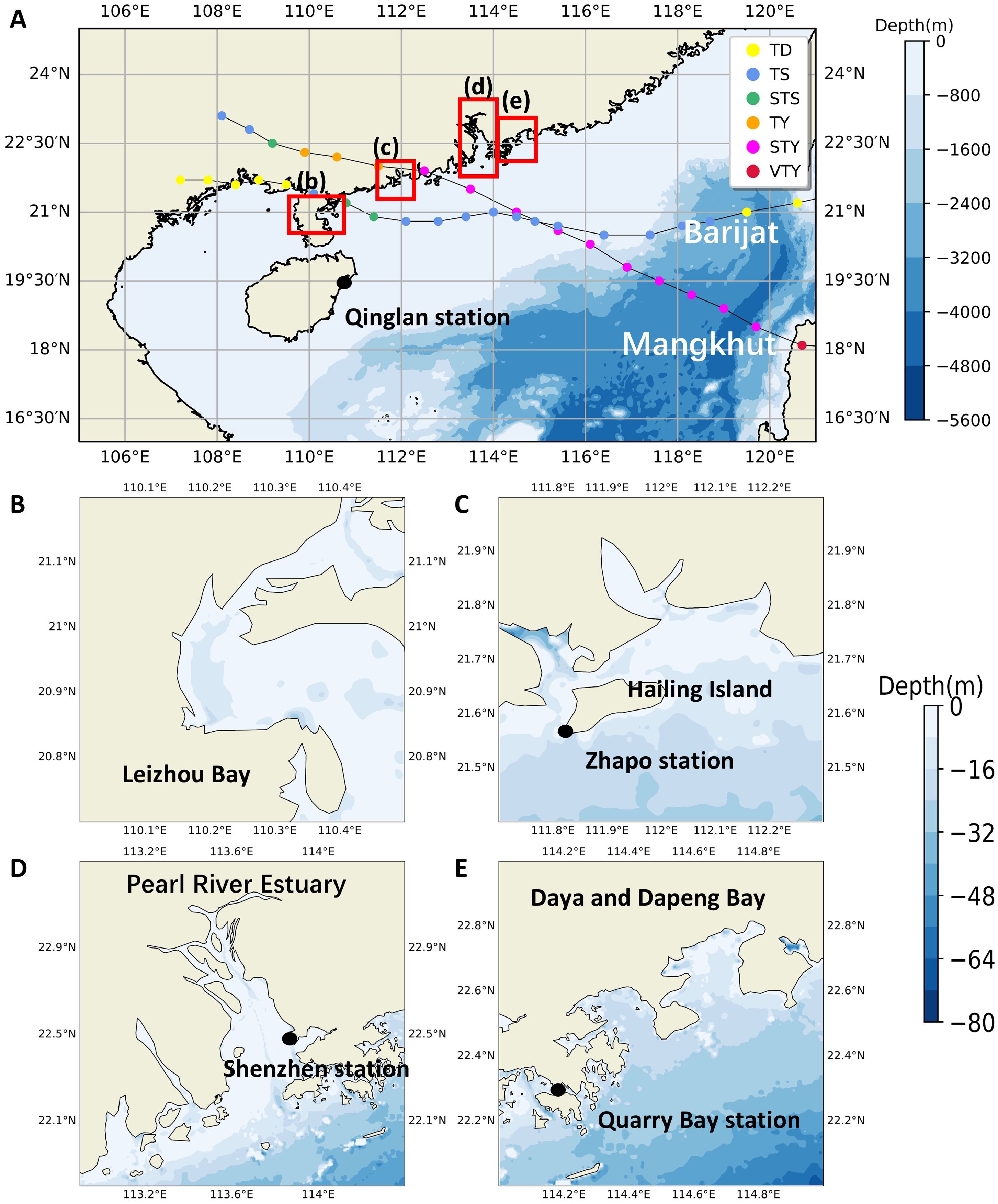
Figure 2. A topographic and bathymetric map of the NSCS and the four main bay regions. (A) shows the model’s domain and the designated areas highlighted within red rectangles from left to right: (B) Leizhou Bay, (C) Hailing Island, (D) Pearl River Estuary, and (E) Daya Bay and Dapeng Bay. The shading corresponds to the water depths within each respective region, while the black dots represent the locations of the four tidal gauge stations. The two lines and the points in (A) depict the tracks and strengths of Barijat and Mangkhut (2018).

There are few steps we took to ensure the accuracy of our tidal simulations: First, we chose multiple tide gauge stations with reliable and continuous water level records to serve as validation points. Using the t-tide package, we decomposed the water level data from these stations into specific tidal constituents, ensuring we had precise measures of the tidal amplitudes and phases. We then ran a pure tidal simulation using our model and compared the results directly with the observed tidal water levels from the selected stations. The comparison revealed that our model accurately simulates the tidal elevations, with minimal discrepancies in both amplitude and phase. These results confirm that our model can reliably reproduce the key characteristics of the observed tides. Figure 3 shows the comparison results, and the data in Table 1 represent the error analysis of the simulation results.

Figure 3

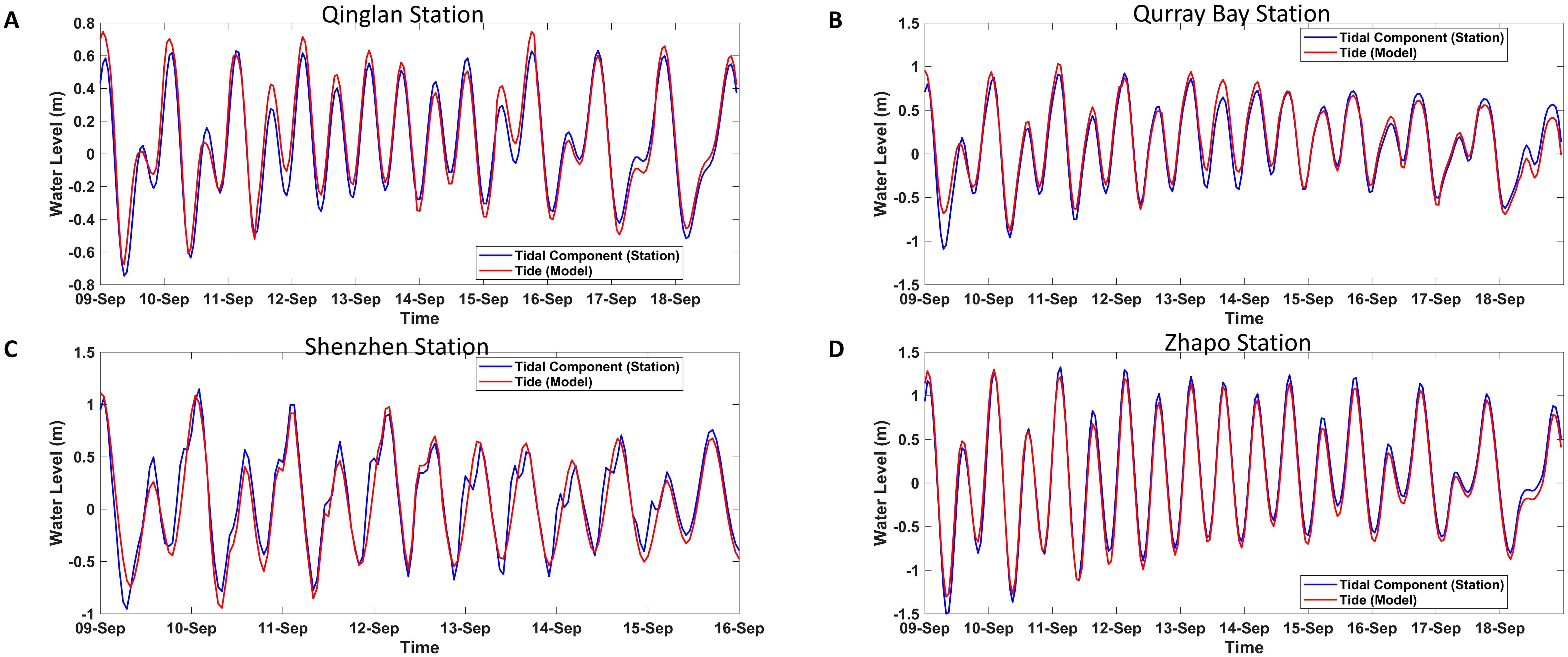
Figure 3. Comparison of the T-tide harmonic analysis results from the observation with the modeled tidal results of Qinglan Station (A), Qurray Bay Station (B), Shenzhen Station (C) and Zhapo Station (D). The red line represents the simulation results, and the blue line represents the T-tide results.

Table 1

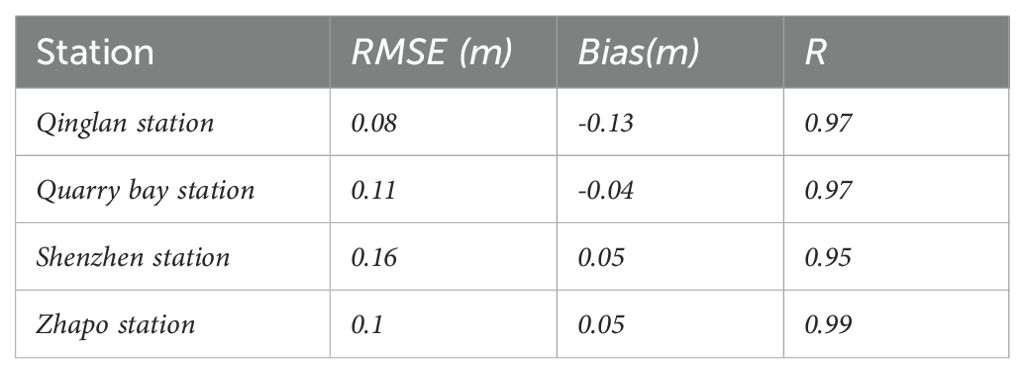
Table 1. Error statistics of tidal simulation results.

We also compared the observed and simulated results of the M2 and K1 tidal constituents at four stations, as shown in Table 2. Notably, the Shenzhen station and Quarry Bay station are located in the Pearl River estuary region, where the river discharge significantly influences tidal dynamics. The use of climatological river discharge data in our simulations may have contributed to the simulation errors observed in this region.

Table 2

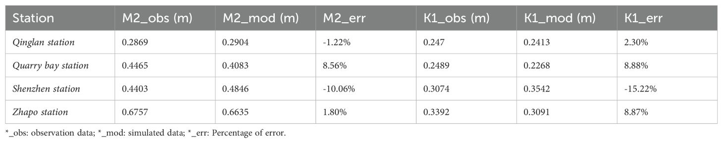
Table 2. The observed and simulated results of the M2 and K1 tidal constituents at the four station.

Figure 4 showcases the observed and simulated results of storm tide duration (September 4th-10th; September 10th-18th) at four stations. In Figure 4, the recording results at the Shenzhen station were terminated on September 16th, and the time corresponds to September 2018 in the UTC+8 time zone. The residual water level in Figure 4 is the total water level minus the monthly mean water level, as below. The light gray shading represents the period during Barijat, while the dark gray shading represents Mangkhut.

Figure 4

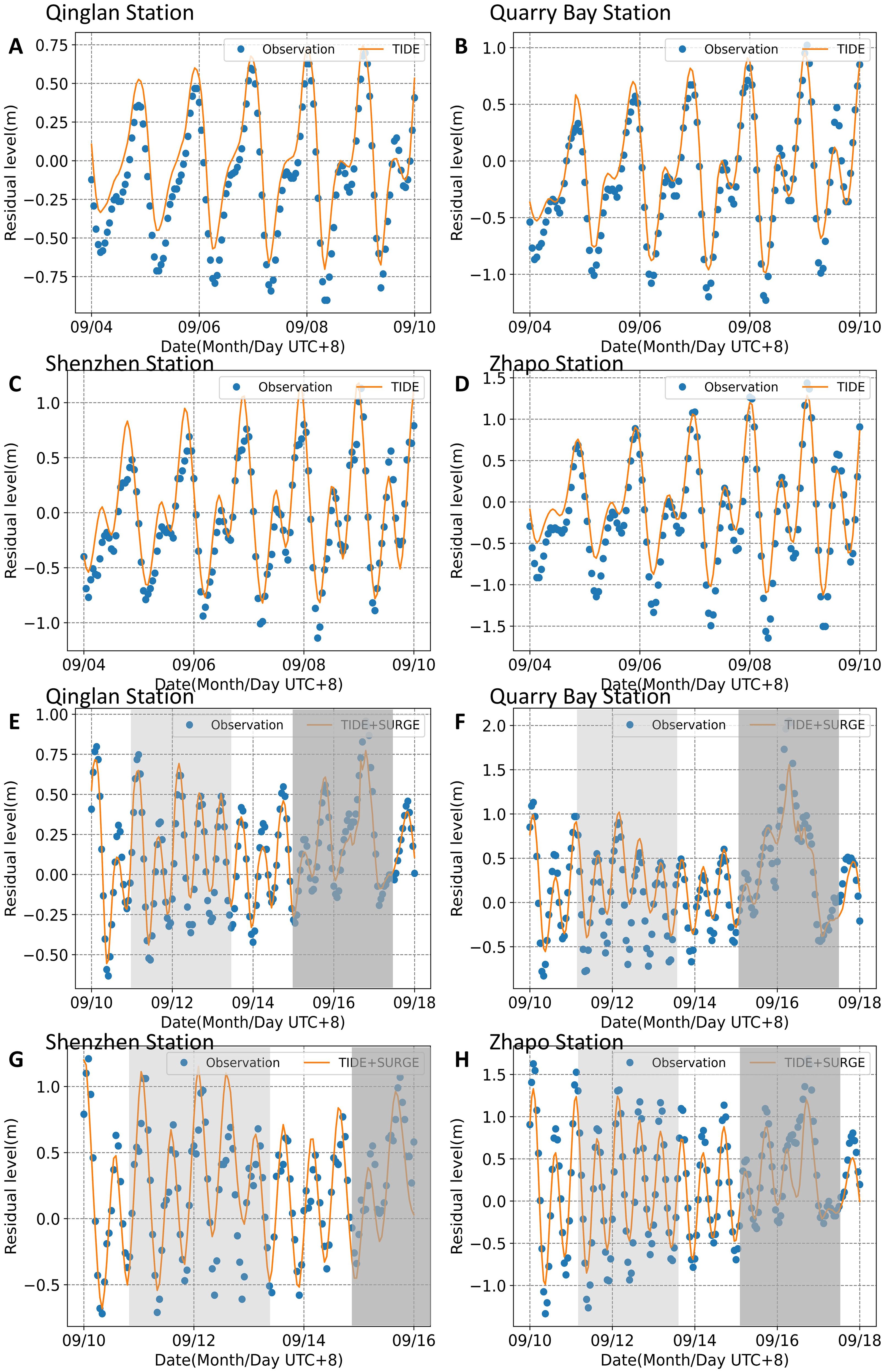
Figure 4. The comparisons between observed water level and ${\zeta }_t$ (A-D); observed water level and ${\zeta }_{st}$ (E-H) at four stations. The light gray and dark gray lines refer to the duration of Barijat and Mangkhut (2018), respectively.

To quantify the model’s skill in simulating water levels in NSCS, three error statistical parameters were calculated.

The root-mean-square error (RMSE):

$\begin{array}{ll}RMSE=\sqrt{\frac{{\sum }_{i=1}^N{(P_i-M_i)}^2}{N}}& (10)\end{array}$

Where $N$ is the number of observations, $M_i$ is the measured value, and $P_i$ is the model-predicted value.

Bias is defined as the mean difference between model predictions and the measurements:

$\begin{array}{ll}Bias=\frac{{\sum }_{i=1}^N(P_i-M_i)}{N} & (11)\end{array}$

The linear correlation coefficient (R) is a measure of the linear relationship between model predictions and the measurements:

$\begin{array}{ll}R=\frac{{\sum }_{i=1}^N(P_i-\overline{P})(M_i-\overline{M})}{\sqrt{\left({\sum }_{i=1}^N{\left(P_i-\overline{P}\right)}^2\right)\left({\sum }_{i=1}^N{(M_i-\overline{M})}^2\right)}}& (12)\end{array}$

The calculated results are shown in Tables 1–4:

Table 3

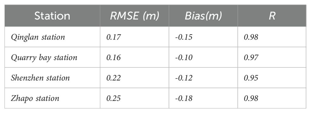
Table 3. Error statistics of storm tide simulation results (September 4^th to 10^th).

Table 4

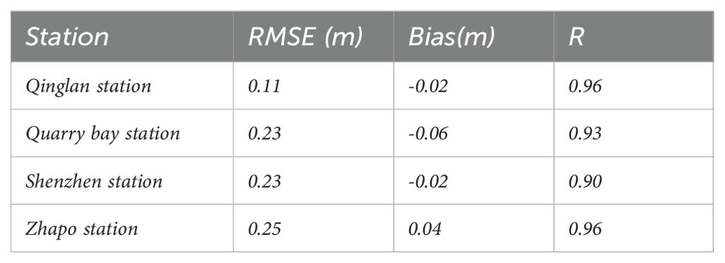
Table 4. Error statistics of storm tide simulation results (September 10^th to 18^th).

The Department of Irrigation and Drainage (DID) Guidelines for Coastal Hydraulic Study had set limitations for water level simulation (DID, 2013). However, DID does not explicitly specify the acceptable limits for RMSE in extreme scenarios like TC occurrences. Therefore, this study applies a general accuracy criterion of 0.3 m for RMSE (Mohd Anuar et al., 2023). Our model effectively capture the process of the storm surge and tide, with model errors remaining within acceptable limits. These discrepancies underscore the model’s capacity to effectively reproduce the storm tide of Barijat and Mangkhut in 2018.

We acknowledge that at some stations, the amplitude error reaches approximately 10%, which may correspondingly result in an error of about 10% in the TSI. Although this error might lead to a slight underestimation of the TSI, it does not influence the variation patterns of TSI at the same location under the impact of different typhoons. These discrepancies between the simulation and the observations are primarily due to the lack of accurate topography and coastline data. In analyzing nearshore tidal levels, shallow water tides also have an impact, with topography being the main influencing factor. Therefore, with the available topography data, we have tried our best to achieve good agreement between our model results and the observed tidal data, which provides a robust foundation for the subsequent analysis of TSI.

4 Result and discussion

Our model results reveal the influence of Barijat and Mangkhut in 2018 on the Northern South China Sea (NSCS) region, particularly along the coast of Guangdong Province, China. These cyclones induced substantial storm surges in the coastal bay areas. According to the tracks of Barijat and Mangkhut (2018), we selected four specific regions (a: Leizhou Bay, b: Hailing Island, c: Pearl River Estuary, d: Daya Bay and Dapeng Bay on both sides of the track to analyze the characteristics of storm surges and TSI in the NSCS during the two TC events. The chosen regions are illustrated in Figure 2, and the maximum surge level shown in Figure 5.

4.1 Storm surge characteristics

The four selected regions encountered varying storm surge impacts during Barijat and Mangkhut (2018). Mangkhut brought stronger surges to these regions. As Mangkhut moved from southeast to northwest, its strong winds initially impacted Daya Bay and Dapeng Bay. By 06:00 on the 16th, the maximum surge of 3.0 meters was recorded in Daya Bay, as shown in Figure 5D. Similarly, the water level in the Pearl River Estuary shows a surge onset from 15:00 on the 15th, driven by eastward winds, with a maximum surge of 2.4 meters in the southwest and a decrease of up to 1.5 meters in the northeast. Hailing Island experienced a double peal surge pattern during Mangkhut’s passage on September 16th. The shifting wind directions caused the storm surge to rise, decline, and resurge. In Leizhou Bay, a similar surge pattern of initial rise, decrease, and resurgence occurred.

Figure 5

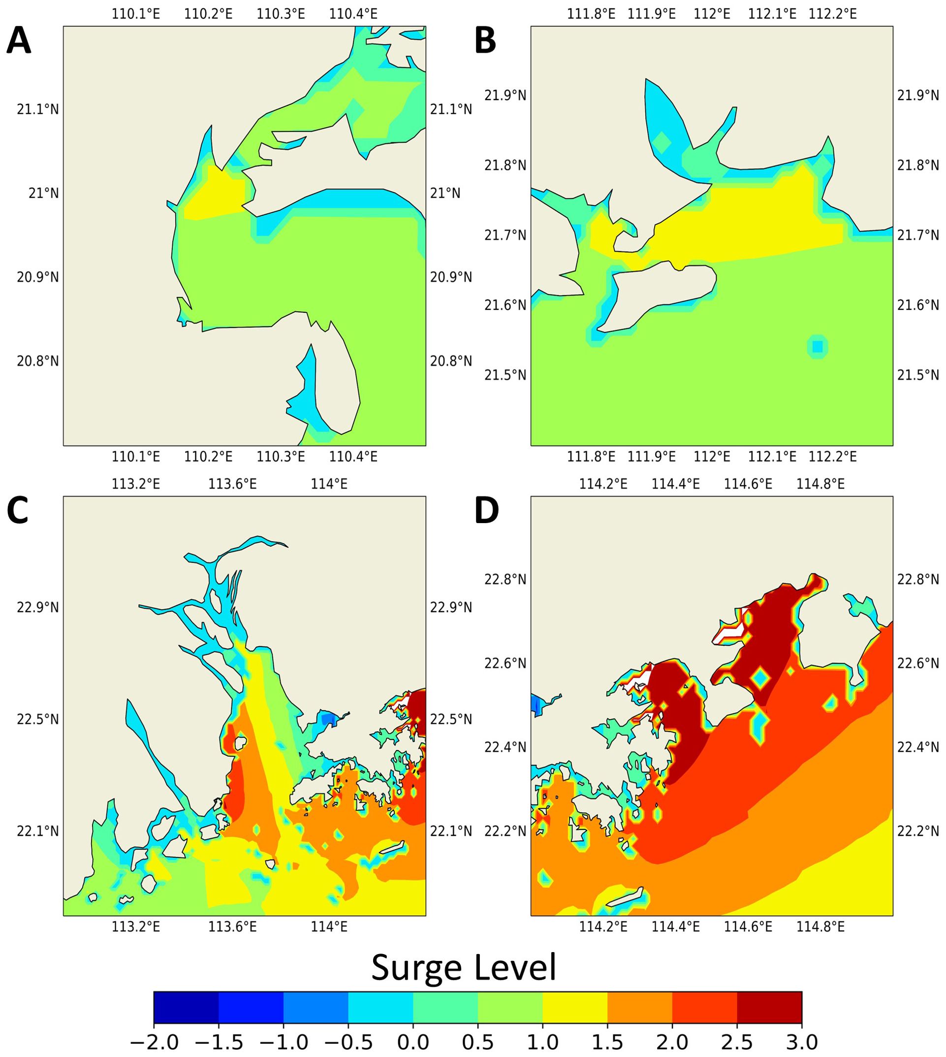
Figure 5. The spatial distribution of maximum ${\zeta }_s$ (water level caused by storm surge) in Leizhou Bay (A), Hailing Island (B), the Pearl River Estuary (C), and Daya Bay and Dapeng Bay (D) during Barijat and Mangkhut (2018), respectively.

Throughout the Barijat period (September 11 to September 13, 2018), storm surges ranging from 0.5 to 1.0 meters were experienced across the regions. Compared to Mangkhut, Barijat had weaker winds and made landfall slightly to the west, resulting in a storm surge below 1 meter in four regions, as depicted in Figure 6. Furthermore, due to the northward tracks of both TCs, the regions on the east side of the Barijat and Mangkhut tracks experienced prevailing easterly or southeasterly winds. Such wind patterns facilitate water accumulation within these bay areas, resulting in a spatial distribution characterized by higher water levels on the left side of the bay and lower levels on the right. As wind speed diminishes, the accumulated water on the left side relaxes towards the right.

Figure 6

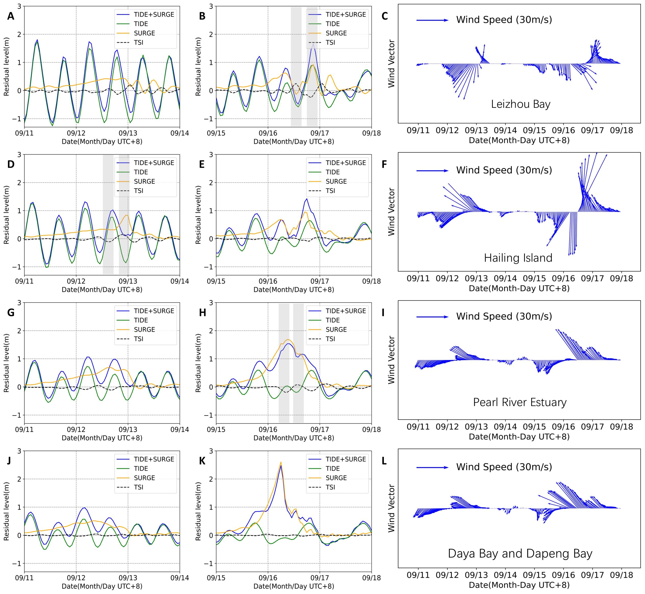
Figure 6. The temporal cross-sections for four distinct regions [Leizhou Bay: (A, B); Hailing Island: (D, E); Pearl River Estuary: (G, H); Daya Bay and Dapeng Bay: (J, K)], corresponding to the impact periods of two TC events. The blue line is the case of TIDE+SURGE, the green line is the case of TIDE, the orange line is the case of SURGE, and the black dotted line illustrates the ${\zeta }_i$. (C, F, I, L) show the wind vector of these regions. The shadows represent six relatively strong TSI events within the three bay areas.

To compare the differences in storm surges caused by two TCs, we use the Hailing Island region as an example. It is situated on the east side of the Barijat tracks and the west side of the Mangkhut tracks (2018). Despite both TCs’ landing sites being very close to Hailing Island, there is a distinctive difference in the surge dynamics observed between the two cyclones. The surge at Hailing Island exhibited an unimodal pattern during Barijat, whereas a double peak surge pattern was observed during Mangkhut. This phenomenon observed at Hailing Island is not unique; bays located on the east side of the tracks of the two TCs exhibited an unimodal characteristic, as shown in Figures 6D, G, H, J, K. Conversely, bays on the west side demonstrated an oscillatory pattern characterized by an initial rise, subsequent decline, and subsequent increase, as illustrated in Figures 6A, B, E. These findings provide insights for the prevention of storm surge disasters.

Assuming a simplified impact zone for the two TCs ranging from 111 to 114 degrees East longitude, it is possible to calculate their respective durations of influence on the Hailing Island area as 13 hours for Barijat and 9 hours for Mangkhut, indicating a notably faster progression speed for Mangkhut. However, as depicted in Figures 6D, E, the durations of storm surge impacts induced by both cyclones appear to be similar. This similarity arises because Mangkhut, characterized by higher wind speeds and lower atmospheric pressures, led to a broader extent of storm surge disasters. This observation underscores the necessity for an extended lead time in storm surge disaster warnings in anticipation of future super typhoon events.

The significance of topography should not be overlooked. As illustrated in Figures 5A, B, the extremities of storm surges are prone to occur on both sides of narrow straits, such as Hailing Island and Leizhou Bay. These areas, due to their constricted topography, experience a “funneling effect,” which leads to greater flow velocities and consequently higher storm surge levels. Certainly, despite the apparent enrichment of storm surge inside and outside the strait as visible from the model, the limited grid resolution may affect the authenticity of the surge distribution due to the sparse number of grid points. Furthermore, a comparison between Daya Bay, Dapeng Bay, and the Pearl River Estuary reveals that, despite the deeper topography of Daya Bay and Dapeng Bay, the southeast-oriented openings of these bays are more conducive to the accumulation of storm surge levels induced by typhoons moving from the southeast to the northwest. Conversely, for the Pearl River Estuary, the currents tend to flow out to the open sea along the western side of the bay.

4.2 Tide-Surge Interactions and its impact

TSI constitutes a challenging aspect of storm surge forecasting, posing significant challenges to accurately predicting storm tides. In the NSCS, long-term influences of TSI have been observed, with records indicating TSI observations at all 12 tide gauge stations in the region (Feng et al., 2015). Four designated regions are utilized to elucidate the characteristics of TSI during Barijat and Mangkhut (2018).

In Figures 6A, B, D, E, G, H, J, K, the black dotted lines represent the variations in ${\zeta }_i$ across specified regions. High ${\zeta }_s$ values are observed in Daya Bay and Dapeng Bay, yet these areas are characterized by the weakest TSI, caused by neap tides with ${\zeta }_t$ fluctuations less than 0.5 meters during the Mangkhut landfall. In the Pearl River Estuary, significant fluctuations in ${\zeta }_i$ are noted, with a maximum increase of 0.11 meters at 03:00 on September 17th and a maximum reduction of 0.19 meters at 08:00 on September 16th. During Barijat in the region around Hailing Island, the maximum ${\zeta }_i$ variations were recorded at 20:00 on September 12th (an increase of 0.19 meters) and at 03:00 on September 13th (a decrease of 0.16 meters). Conversely, TSI in the region around Hailing Island exhibited lesser intensity during Mangkhut, resulting in more minor ${\zeta }_i$ fluctuations. Leizhou Bay experiences pronounced TSI, with an average maximum ${\zeta }_i$ variation of 0.26 meters at 01:00 on September 17th, contributing to -10% of ${\zeta }_{st}$ at peak times. During the peak time of storm surges, TSI predominantly contributes negatively, with a contribution rate ranging between -5 to -20 percent. An exception is observed in Hailing Island during the Barijat period, where the positive TSI coincides with low tide, illustrating the complex relationship between TSI and tide. In order to see the importance of TSI, we calculate the TSI contribution at the peak time of storm surge.

$\begin{array}{ll}\text{Ptc}\left(\frac{B}{M}\right)=\frac{{\zeta }_i}{{\zeta }_s}\times 100\%& (13)\end{array}$

Where Ptc(B/M) is the Peak time contribution (Barijat/Mangkhut).

The calculated results are shown in Table 5:

Table 5

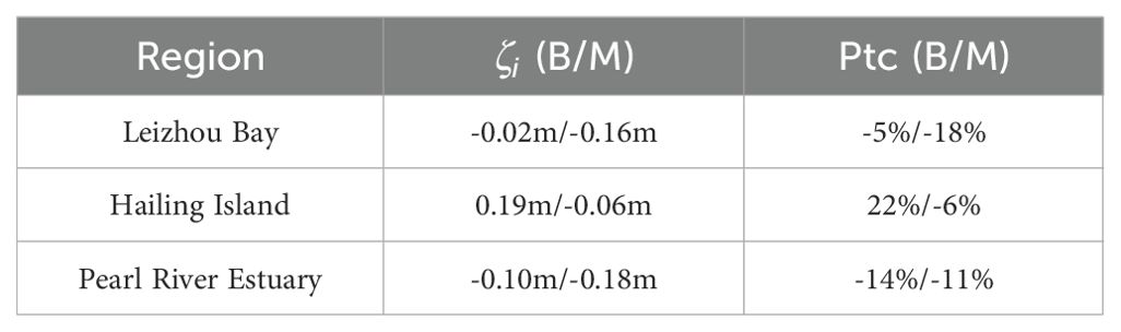
Table 5. Peak time contribution of TSI during Barijat (B) and Mangkhut (M) in 2018.

Figure 6 presents a comparative analysis of ${\zeta }_i$ during Barijat and Mangkhut (2018) across four regions. Despite lower wind speeds in Barijat compared to Mangkhut, an equivalence in induced TSI was observed, underscoring the influence of factors other than storm intensity on TSI. The modulation of tide by storm surges, and vice versa, has been a subject of observation and analysis in various studies (Brown et al., 2010; Antony and Unnikrishnan, 2013; Feng et al., 2019). This phenomenon was particularly evident during Mangkhut, where a strong surge resulted in a weak tide in Daya Bay and Dapeng Bay. Specifically, storm surge modulation on tides is reflected in tidal phase shifts and changes in tidal amplitude, which vary depending on location, water depth, and wind direction, with marked variations evident in shallow waters (Jones and Davies, 2007). These modulations will be reflected in the form of TSI. Based on Figure 6, it can be observed that storm surges serve as a prerequisite condition for the generation of TSI, yet the amplitude and polarity of TSI are primarily determined by the fluctuations in tidal forces. The amplitude of TSI increases in conjunction with the augmentation of tidal amplitude, and it is noted that the peak values do not correspond on a one-to-one basis. The impact of tides on TSI was dominated, with negative ${\zeta }_i$ observed during rising tides and positive ${\zeta }_i$ during falling tides. This phenomenon aligns with findings from previous research (Rego and Li, 2010; Antony et al., 2020). Hailing Island serves as a prime example of the predominant influence of tidal forces on the TSI. Despite comparable levels of storm surge, the tidal amplitude during the Barijat period was relatively larger compared to that during the Mangkhut period, consequently leading to a greater TSI.

Figure 7 demonstrates the influence of tide and surge on the magnitude of TSI and their correlation, standard deviation, andreference during Barijat and Mangkhut (2018) in Leizhou Bay, Hailing Island, and Pearl River Estuary. Daya Bay and Dapeng Bay have been excluded from further TSI discussions for their weak TSI. It is shown that the positive TSI during Mangkhut was more robust compared to that during Barijat. Additionally, TSI exhibits a negative correlation with tide and a positive correlation with surge. Although the impact of surge on TSI is significant, the effect of tide is dominant, with a higher correlation with TSI, as indicated in Figures 7B, D. This emphasizes the crucial need for adequate attention to the tide effect in nearshore storm surge disaster prevention.

Figure 7

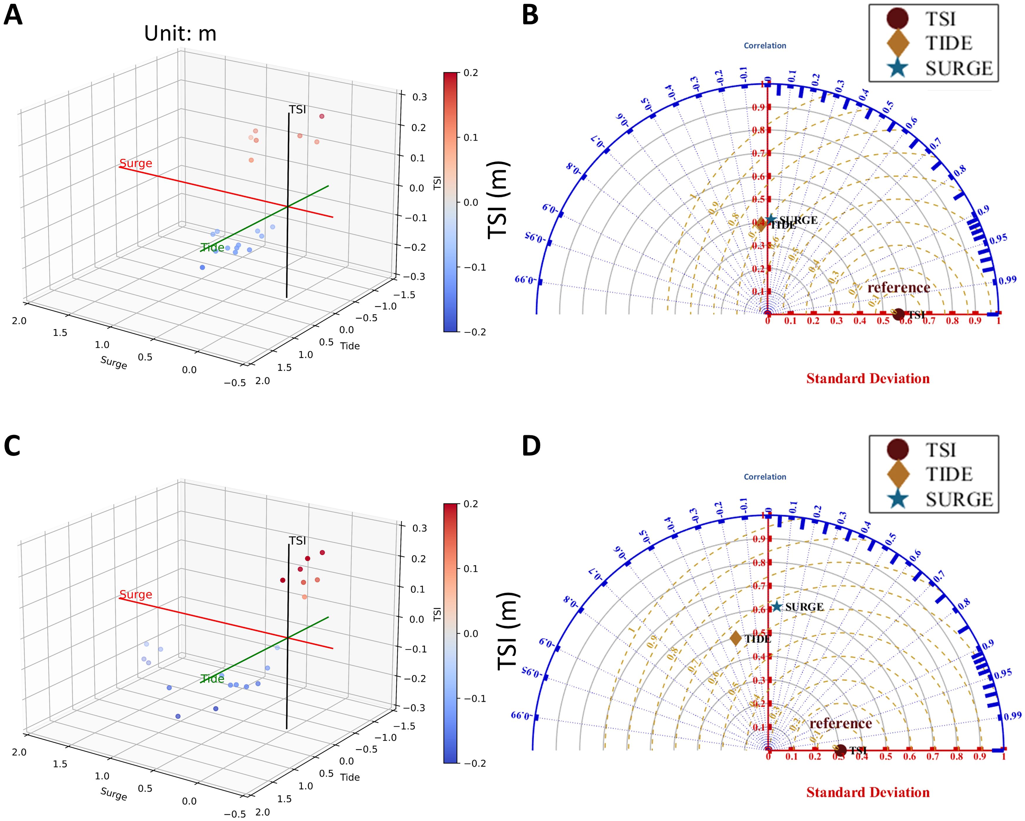
Figure 7. The influence of tide and surge on the magnitude of TSI and their Correlation, Standard Deviation, and Reference during Barijat (A, B) and Mangkhut (2018) (C, D). The absolute values of ${\zeta }_i$ exceeded 0.1 meters in three bay areas between Barijat and Mangkhut are shown. The red dots represent positive TSI, the blue dots represent negative TSI, and the color bar indicates the strength of the TSI in (A, C).

The primary cause of ${\zeta }_i$ has been identified as TSI currents (Khalilabadi, 2016). To validate their relationship, time-series graphs have been plotted, demonstrating the correlation between ${\zeta }_i$ and TSI effective currents, as depicted in Figures 8C, F, I. Given the diverse flow directions of TSI currents entering the bay area, we propose effective currents for different regions. For instance, in the Pearl River Estuary, considering its geographical features and local wind directions, we designated TSI currents within the range of 60-120 degrees as effective currents contributing positively to ${\zeta }_i$ (i.e., inflowing currents into the Pearl River Estuary, Figure 8H), while currents from other directions were deemed negatively contributing (i.e., outflowing currents from the Pearl River Estuary). A two-hour lag correlation between TSI currents and ${\zeta }_i$ with a correlation coefficient of 0.76. Similarly, based on the geographical characteristics of Hailing Island, we selected currents in the 120-180-degree direction as effective currents contributing positively, as shown in Figure 8E, yielding a two-hour lag correlation coefficient of 0.79 between TSI currents and ${\zeta }_i$. In the Leizhou Bay area, predominantly oriented east-west, currents in the 90-180-degree direction (Figure 8B) were designated as positive contributors, with other directions as negative contributors, causing a two-hour lag correlation coefficient of 0.83 between TSI effective currents and ${\zeta }_i$. These correlation analyses have tentatively established the significance of TSI effective currents in influencing ${\zeta }_i$.

Figure 8

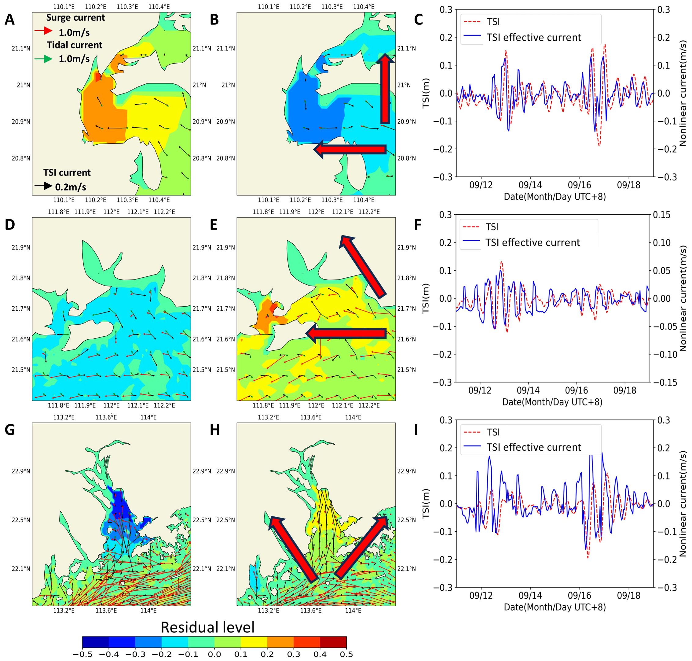
Figure 8. The ${\text{ζ}}_{\text{i}}$ (A, B, D, E, G, H) superimposed with the corresponding currents at the peak time of six strong TSI events. The panels (C, F, I) show the time series of TSI water levels and currents. The angle between the big red arrows represents the direction of the selected TSI effective currents entering the bay area.

The relationship of TSI, surge, and tide can be further analyzed from the perspective of the currents field. Figures 8A, B, D, E, G, H show the corresponding variations in the currents field for the six TSI events. For instance, in Figures 8B, D, G, these three negative TSI processes correspond to TSI currents flowing outward from the bay areas, while tide currents and surge currents are directed inward. Similarly, in Figures 8A, E, H, these three positive TSI events correspond to TSI currents flowing inward into the bay area, while tide currents and surge currents are directed outward. These observations suggest that TSI currents act as compensating flows for tide and surge currents, exhibiting a negative correlation with both. Furthermore, when comparing the changes in storm tide currents with TSI currents, it is noted that TSI currents serve as compensating flows for storm tide currents, with their magnitude being approximately 10 percent of that of the storm tide currents.

A comparison between Leizhou Bay and Hailing Island readily demonstrates the significant role that topography plays in the formation of TSI. Topography dictates the changes in the direction of nearshore currents and, along with storm surges, predominantly influences the generation of TSI currents. As illustrated in Figure 8, TSI currents are manifested as compensatory flows of tidal currents and storm surges, thus when the tidal currents and storm surges move in the same direction, the TSI currents are at their strongest. This highlights the importance of topographic effects on TSI.

4.3 Dynamic mechanism of TSI

According to the methods mentioned in Section 2.4, we perform the following analysis of the TSI mechanisms:

The combined effects of various terms have been comprehensively assessed in Equations 8 and 9 under consideration. A precise and comprehensive evaluation of the nonlinear effects of TSI has been conducted in the Pearl River Estuary, Hailing Island, and Leizhou Bay regions. Among these terms, the baroclinic pressure gradient term is negligible in nearshore regions. The surface wind stress term in case TIDE+SURGE is equal in magnitude to that of case SURGE, while in case TIDE, the surface wind stress term is zero. Therefore, their difference is also zero. Thus, we focus on analyzing the nonlinear advection and diffusion terms, Coriolis force terms, barotropic pressure gradient terms, bottom friction stress terms, and trend terms ($\frac{\partial \overline{U}D}{\partial t}$). The trend term is equal to the sum of six terms, as depicted in Figures 9 and 10A–C.

Figure 9

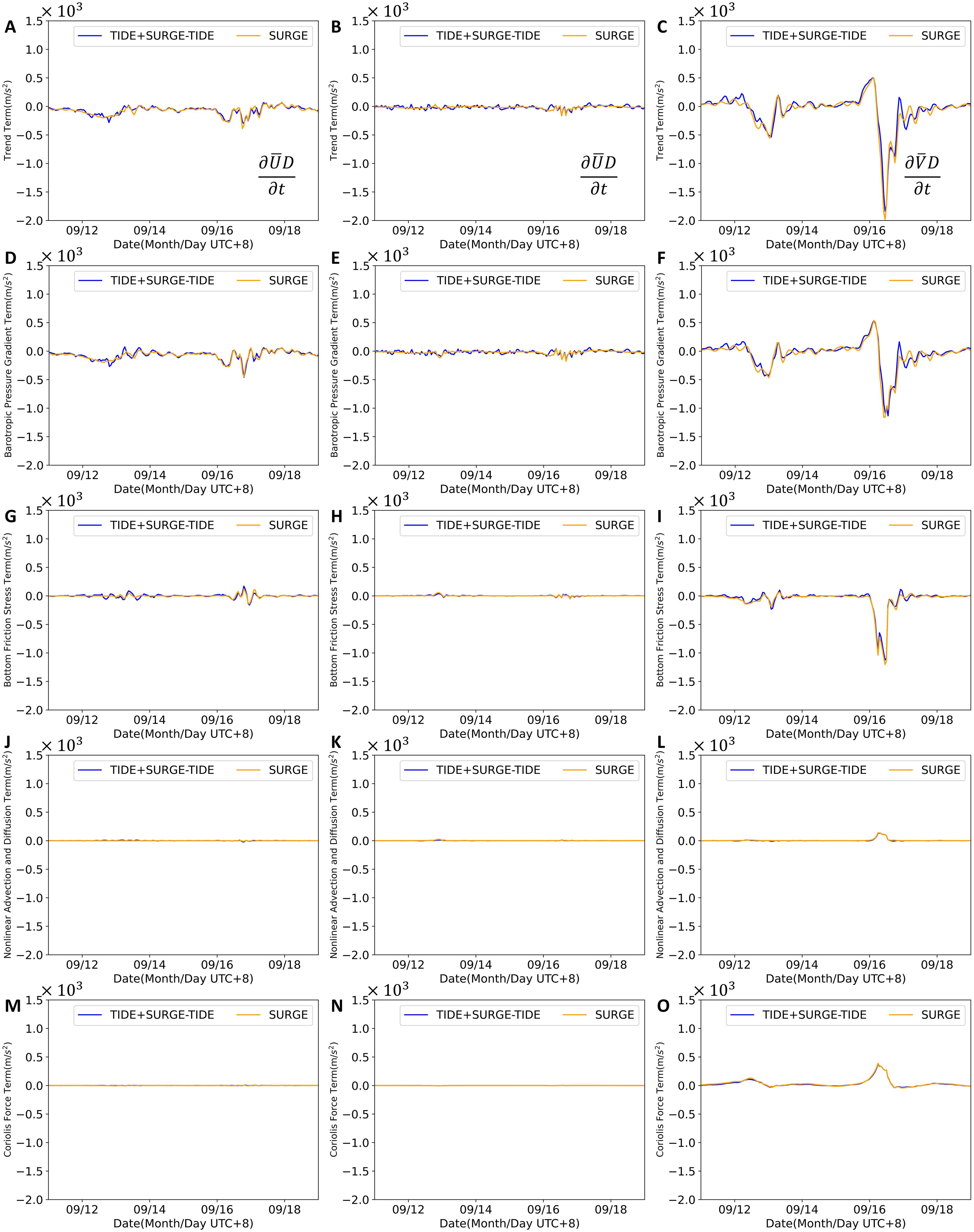
Figure 9. Time series of the trend terms (A–C), barotropic pressure gradient terms (D–F), bottom friction stress terms (G–I), nonlinear advection and diffusion terms (J–L) and Coriolis force terms (M–O) in Leizhou Bay, Hailing Island, and Pearl River Estuary, respectively. The SURGE case is shown by the orange line, and the difference between TIDE+SURGE and TIDE cases is shown by the blue line.

Figure 10

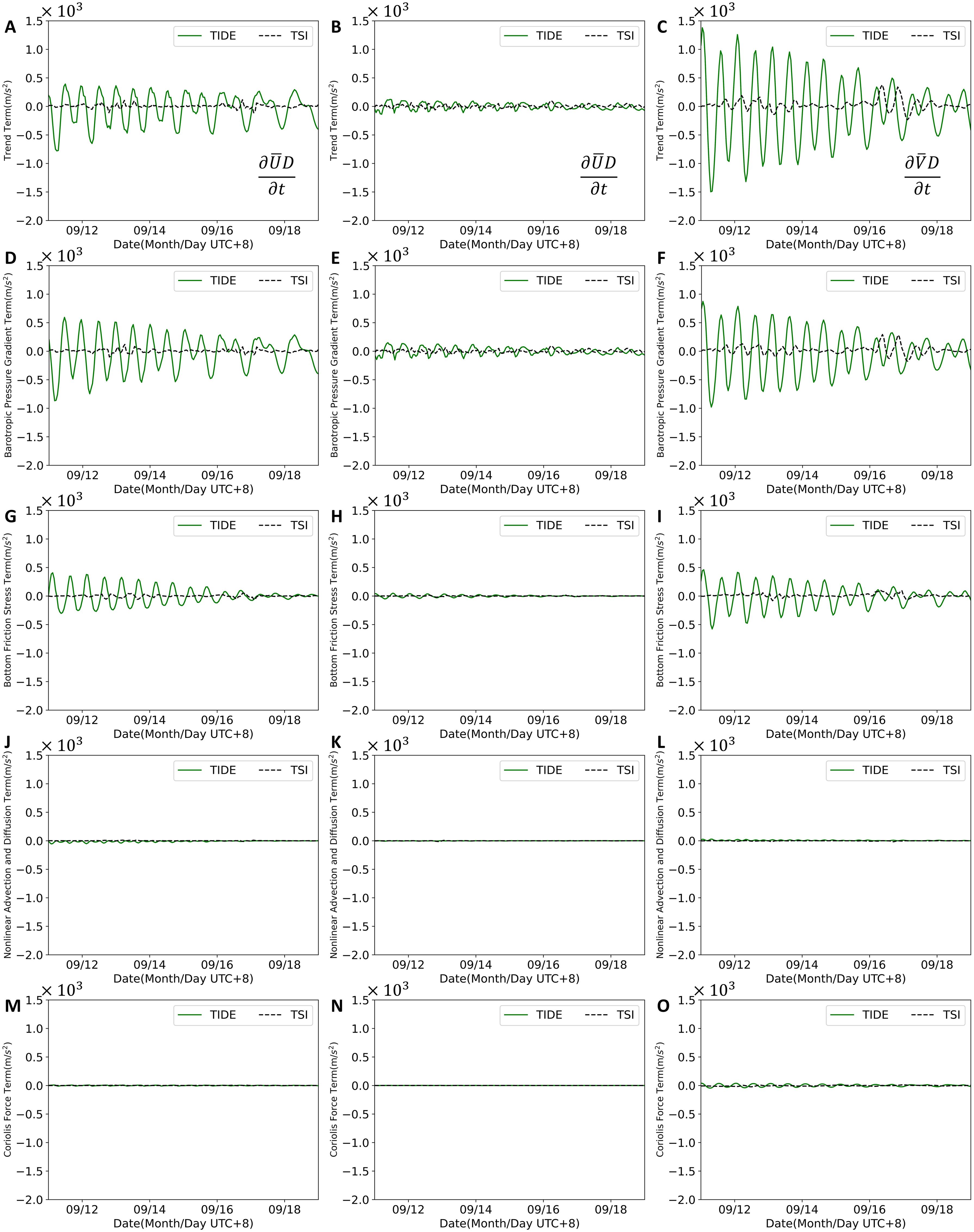
Figure 10. Time series of the trend terms (A–C), barotropic pressure gradient terms (D–F), bottom friction stress terms (G–I), nonlinear advection and diffusion terms (J–L) and Coriolis force terms (M–O) in Leizhou Bay, Hailing Island, and Pearl River Estuary, respectively. The TIDE case is shown by the green line, and the TSI is shown by the black dotted line

Figures 9 and 10D–F illustrate the barotropic pressure gradient term of the equations, with the two peaks corresponding to the two TCs. It is evident that among the four terms, the barotropic pressure gradient term exhibits the largest amplitude, suggesting that it is the dominant factor in TSI currents. Xing et al. (2011) indicated that TSI is primarily balanced between the barotropic pressure gradient term and the bottom friction term in shallow waters. This finding aligns with our research, as the barotropic pressure gradient term dominates the three bay areas. The nonlinear effect of the barotropic pressure gradient term is readily understandable. When the tide recedes, the water level in the bay area drops correspondingly, creating a barotropic pressure gradient force between the higher water level outside the bay and the lower water level within it. This results in TSI onshore currents flowing into the bay area as a compensating mechanism. Conversely, when the water level inside the bay is higher, the barotropic pressure gradient force reverses, causing TSI currents to flow outward. This phenomenon corresponds with the observed decrease in ${\zeta }_i$ during high tide and the increase during low tide.

The bottom friction stress term of the equations is represented in Figures 9 and 10G–I. Its amplitude is also significant, second only to the barotropic pressure gradient term, nearly matching it in Leizhou Bay. The bottom friction stress term is generated due to friction between the current and the seabed. Etala (2009) discusses how bottom friction stress is the primary effect of TSI in the Bahía Blanca estuary channel. The presence of the bottom friction stress term also elucidates why regions with more considerable ${\zeta }_i$ variations are mainly concentrated in shallow coastal areas. In deeper waters, the bottom friction stress term is relatively minor, leading to correspondingly smaller TSI values (Idier et al., 2019). Leizhou Bay, Hailing Island, and Pearl River Estuary are shallower than Daya and Dapeng Bay and exhibit stronger nonlinear bottom friction forces.

Figures 9 and 10J–O represent the nonlinear advection and diffusion term, and the Coriolis force term of the equations, respectively. In comparison to the barotropic pressure gradient term and bottom friction stress terms, these two terms are negligible. Furthermore, the small magnitudes of the Coriolis force term are attributed to the small-scale nature of the currents. These terms make minimal contributions to the TSI currents.

From Figures 6 and 9, it is evident that the storm surge caused by Barijat had minimal impact on the storm surge induced by Typhoon Mangkhut. After the weakening of the wind force, both the water level and the flow field adjusted rapidly, completing the adjustment within a few hours. This indicates that the amplification of storm surge disasters due to sequential tropical cyclones does not stem from changes in the background field of the areas recently affected by a storm surge, making them more susceptible to further storm surges.

In our investigation of four distinct regions, the region around Hailing Island emerged as an exceptional area. The island experienced landfalls of two separate TCs on its west and east sides, generating storm surge peak levels of comparable magnitude. Therefore, we have rendered a spectral analysis for three time-series (time-series in Figure 9B and green line in Figure 10B) in Hailing Island to see how TSI influences the surge during Barijat and Mangkhut. During the period of Barijat, the tide is predominantly characterized by semidiurnal tides, along with high-frequency tidal signals with periods of six hours or even shorter. Figure 11A shows that the surge does not alter the semidiurnal tides. However, it influences the high-frequency processes interacting with the topography. This interaction diminishes the signals with six-hour and three-hour periods while amplifying the variations with a higher frequency at a two-hour period. During the period of Mangkhut, the tides were predominantly characterized by 12-hour and 6-hour periods, with high-frequency tides primarily occurring on a 6-hour basis. The surge contributed to the enhancement of processes with a 3-hour period. It was observed that the TSI caused the surge to carry high-frequency tidal signals during Barijat, evidenced by signals of two to six-hour periods and diminished energy at lower frequencies (periods longer than 9 hours), indicative of an energy shift from low to high frequencies, as shown in Figure 11A. However, during Mangkhut, the TSI reduced this energy component at the peak frequency of surge corresponding to a 200-minute period and enhanced the energy of surge corresponding to a 300 to 500-minute period, as delineated in Figure 11B.

Figure 11

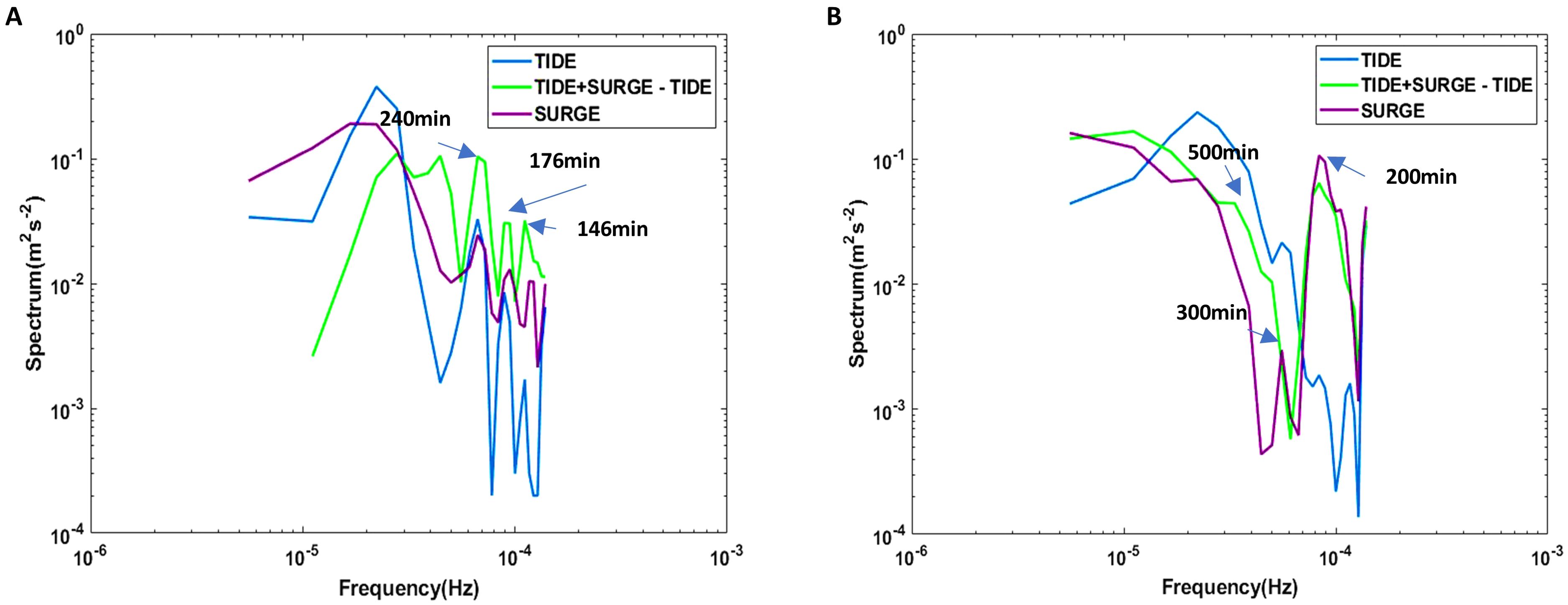
Figure 11. The spectral analysis during the Barijat (A) and Mangkhut (B) periods results from three time series in Figures 9B and 10B.

As Hailing Island was located on the east side of Mangkhut’s track, the double peak storm surge pattern during the typhoon led to substantial short-term variations in the flow field. Consequently, this manifested as high-frequency storm surge signals in the spectral frequency analysis. This high-frequency surge signal exceeds the frequency of tide. Therefore, TSI shows the effect of diminishing the high-frequency surge in Mangkhut. On the other hand, Hailing Island was positioned on the west side of Barijat’s track, experiencing a more stable storm surge during the typhoon, and the variations of flow field were also more stable. Besides, the tide tidal signal had a higher frequency than that during Mangkhut. Therefore, TSI resulted in the surge carrying high-frequency tidal signals. Due to the primary modulation of the TSI by tides, the frequency of TSI is similar to that of tidal frequencies. Under the modulation of TSI, the storm surge carries signals of higher or lower frequency than the tides, depending on the intrinsic signal frequency of the storm surge itself. This also exemplifies the modulatory effect of TSI on storm surges.

5 Conclusions

In this case study, the Princeton Ocean Model (POM) was employed to simulate storm surges during Barijat and Mangkhut in the NSCS in 2018. A comparative analysis was conducted of the characteristics of storm surges in Leizhou Bay, Hailing Island, Pearl River Estuary, and Daya Bay and Dapeng Bay in the NSCS, and a detailed investigation was carried out into the influences and physical mechanisms of the TSI.

The main conclusions are as follows:

1. TSI had considerable effects in the Pearl River Estuary, Hailing Island, and Leizhou Bay regions, resulting in TSI variations within the range of -0.3 to 0.3 meters. At peak times, the TSI consistently contributed negatively to the storm surge, ranging from approximately -5% to -20%.

2. As the TCs moved from southeast to northwest, the storm surge on the east side of its track in the NSCS increased continuously. In contrast, the storm surge on the west side of its track showed an oscillating pattern characterized by an initial rise, decrease, and resurgence pattern.

3. By comparing the variations of TSI in the four bay areas during Barijat and Mangkhut (2018), it is shown that stronger storm surges contribute to enhanced TSI. However, TSI is mainly dominated by tidal dynamics, manifested as a negative TSI during rising tides and a positive pattern during falling tides.

4. The variations in ${\zeta }_i$ within the bay areas are primarily associated with TSI effective currents. Further dynamic analysis of the mechanisms of TSI revealed that variations in these currents were predominantly driven by the barotropic pressure gradient term, with the bottom friction stress term playing a secondary role.

5. In Hailing Island, TSI caused the surge to carry high-frequency tidal signals during Barijat. For the more intense Typhoon Mangkhut, however, a double peak surge pattern will cause surge energy to concentrate at a higher frequency. In this case, TSI diminished the energy of high-frequency surge.

This study provides a comprehensive understanding of the complex interactions between tidal dynamics and storm surges in the NSCS. Our findings underscore the importance of considering TSI when assessing storm surge phenomena during typhoon events in coastal regions.

Data availability statement

The raw data supporting the conclusions of this article will be made available by the authors, without undue reservation.

Author contributions

YC: Conceptualization, Data curation, Formal analysis, Investigation, Methodology, Validation, Visualization, Writing – original draft. YM: Formal analysis, Validation, Visualization, Writing – review & editing. PX: Funding acquisition, Methodology, Software, Writing – review & editing. YZ: Funding acquisition, Resources, Supervision, Writing – review & editing. YL: Funding acquisition, Resources, Supervision, Writing – review & editing, Conceptualization, Data curation, Project administration, Software.

Funding

The author(s) declare financial support was received for the research, authorship, and/or publication of this article. This research was funded by the Major Projects of the National Natural Science Foun-dation of China (U21A6001, 41890851, 42206220), Guangdong Basic and Applied Basic Research Foundation (2024B1515040024, 2024B1515020037, 2023A1515012691), the Southern Marine Science and Engineering Guangdong Laboratory (Guangzhou) (2019BT02H594), the Chinese Academy of Sciences (SCSIO202204, and SCSIO202201). The analysis in this study is supported by the High-Performance Computing Cluster at the South China Sea Institute of Oceanology.

Conflict of interest

The authors declare that the research was conducted in the absence of any commercial or financial relationships that could be construed as a potential conflict of interest.

Publisher’s note

All claims expressed in this article are solely those of the authors and do not necessarily represent those of their affiliated organizations, or those of the publisher, the editors and the reviewers. Any product that may be evaluated in this article, or claim that may be made by its manufacturer, is not guaranteed or endorsed by the publisher.

References

Antony C., Unnikrishnan A. S. (2013). Observed characteristics of tide-surge interaction along the east coast of India and the head of Bay of Bengal. Estuarine Coast. Shelf Sci. 131, 6–11. doi: 10.1016/j.ecss.2013.08.004

Crossref Full Text | Google Scholar

Antony C., Unnikrishnan A. S., Krien Y., Murty P. L. N., Samiksha S. V., Islam A. K. M. S. (2020). Tide–surge interaction at the head of the Bay of Bengal during Cyclone Aila. Region. Stud. Mar. Sci. 35, 101133. doi: 10.1016/j.rsma.2020.101133

Crossref Full Text | Google Scholar

As-Salek J. A. (1998). Coastal trapping and funneling effects on storm surges in the meghna estuary in relation to cyclones hitting Noakhali–Cox’s bazar coast of Bangladesh. J. Phys. Oceanogr. 28, 227–249. doi: 10.1175/1520-0485(1998)028<0227:CTAFEO>2.0.CO;2

Crossref Full Text | Google Scholar

As-Salek J. A., Yasuda T. (2001). Tide–surge interaction in the meghna estuary: most severe conditions. J. Phys. Oceanogr. 31, 3059–3072. doi: 10.1175/1520-0485(2001)031<3059:TSIITM>2.0.CO;2

Crossref Full Text | Google Scholar

Becker J. J., Sandwell D. T., Smith W. H. F., Braud J., Binder B., Depner J., et al. (2009). Global bathymetry and elevation data at 30 arc seconds resolution: SRTM30_PLUS. Mar. Geodesy 32, 355–371. doi: 10.1080/01490410903297766

Crossref Full Text | Google Scholar

Bernier N. B., Thompson K. R. (2007). Tide-surge interaction off the east coast of Canada and northeastern United States. J. Geophys. Res. 112, C06008. doi: 10.1029/2006JC003793

Crossref Full Text | Google Scholar

Brown J. M., Souza A. J., Wolf J. (2010). An investigation of recent decadal-scale storm events in the eastern Irish Sea. J. Geophys. Res. 115, C05018. doi: 10.1029/2009JC005662

Crossref Full Text | Google Scholar

Caldwell P. C., Merrifield M. A., Thompson P. R. (2015). Sea level measured by tide gauges from global oceans — the Joint Archive for Sea Level holdings (NCEI Accession 0019568), Version 5.5, NOAA (Hawaii, America: National Centers for Environmental Information, Dataset). doi: 10.7289/V5V40S7W at https://www.ncei.noaa.gov/access/metadata/landing-page/bin/iso?id=gov.noaa.nodc:JIMAR-JASL.

Crossref Full Text | Google Scholar

Choi B. H., Eum H. M., Woo S. B. (2003). A synchronously coupled tide–wave–surge model of the Yellow Sea. Coast. Eng. 47, 381–398. doi: 10.1016/S0378-3839(02)00143-6

Crossref Full Text | Google Scholar

CODMEWTL (China’s Ocean Disaster Monitoring and Early Warning Technology Laboratory). (2019). China’s Ocean Disaster Re-port, (2018) (Beijing: China Ocean Press).

Google Scholar

DID. (2013). Guidelines for Preparation of Coastal Engineering Hydraulic Study and Impact Evaluation (Kuala Lumpur, Malaysia: Jabatan Pengairan dan Saliran (JPS).

Google Scholar

Dinápoli M. G., Simionato C. G., Moreira D. (2020). Nonlinear tide-surge interactions in the Río de la Plata Estuary. Estuarine Coast. Shelf Sci. 241, 106834. doi: 10.1016/j.ecss.2020.106834

Crossref Full Text | Google Scholar

Duan Y., Zhu J., Qin Z., Gong M. (2015). A high-resolution numerical storm surge model in the Changjiang river estuary and its application. Acta Oceanol. Sin. 27, 11–19. doi: 10.3321/j.issn:0253-4193.2005.03.002

Crossref Full Text | Google Scholar

Egbert G. D., Erofeeva S. Y. (2002). Efficient inverse modeling of Barotropic ocean tides. J. Atmos. Ocean. Technol. 19, 183–204. doi: 10.1175/1520-0426(2002)019<0183:EIMOBO>2.0.CO;2

Crossref Full Text | Google Scholar

Etala P. (2009). Dynamic issues in the SE South America storm surge modeling. Nat. Hazards 51, 79–95. doi: 10.1007/s11069-009-9390-3

Crossref Full Text | Google Scholar

Feng J., Jiang W., Li D., Liu Q., Wang H., Liu K. (2019). Characteristics of tide–surge interaction and its roles in the distribution of surge residuals along the coast of China. J. Oceanogr. 75, 225–234. doi: 10.1007/s10872-018-0495-8

Crossref Full Text | Google Scholar

Feng J., Von Storch H., Jiang W., Weisse R. (2015). Assessing changes in extreme sea levels along the coast of C hina. J. Geophys. Res. Oceans 120, 8039–8051. doi: 10.1002/2015JC011336

Crossref Full Text | Google Scholar

Flanders Marine Institute (VLIZ), Intergovernmental Oceanographic Commission (IOC). (2024). Sea level station monitoring facility. Available online at: http://www.ioc-sealevelmonitoring.org (Accessed January 01, 2022).

Google Scholar

Gao Y., Wang X., Dong C., Ren J., Zhang Q., Huang Y. (2024). Characteristics and influencing factors of storm surge-induced salinity augmentation in the Pearl river estuary, South China. Sustainability 16, 2254. doi: 10.3390/su16062254

Crossref Full Text | Google Scholar

GEBCO Bathymetric Compilation Group. (2019). The GEBCO_2019 Grid. A continuous terrain model of the global oceans and land. UK: British Oceanographic Data Centre, National Oceanography Centre, NERC. doi: 10.5285/836f016a-33be-6ddc-e053-6c86abc0788e

Crossref Full Text | Google Scholar

Genovese E., Green C. (2015). Assessment of storm surge damage to coastal settlements in Southeast Florida. J. Risk Res. 18, 407–427. doi: 10.1080/13669877.2014.896400

Crossref Full Text | Google Scholar

Hersbach H., Bell B., Berrisford P., Hirahara S., Horányi A., Muñoz-Sabater J., et al. (2017). Complete ERA5 from 1940: Fifth generation of ECMWF atmospheric rea-nalyses of the global climate. Copernicus Climate Change Service (C3S) Data Store (CDS). doi: 10.24381/cds.143582cf

Crossref Full Text | Google Scholar

Holland G. J. (1980). An analytic model of the wind and pressure profiles in hurricanes. Mon. Wea. Rev. 108, 1212–1218. doi: 10.1175/1520-0493(1980)108<1212:AAMOTW>2.0.CO;2

Crossref Full Text | Google Scholar

Horsburgh K. J., Wilson C. (2007). Tide-surge interaction and its role in the distribution of surge residuals in the North Sea. J. Geophys. Res. 112, 2006JC004033. doi: 10.1029/2006JC004033

Crossref Full Text | Google Scholar

Hu T.-Y., Ho W.-M. (2015). Prediction of the impact of typhoons on transportation networks with support vector regression. J. Transp. Eng. 141, 04014089. doi: 10.1061/(ASCE)TE.1943-5436.0000759

Crossref Full Text | Google Scholar

Huang X., Wang N. (2024). An adaptive nested dynamic downscaling strategy of wind-field for real-time risk forecast of power transmission systems during tropical cyclones. Reliabil. Eng. Sys. Saf. 242, 109731. doi: 10.1016/j.ress.2023.109731

Crossref Full Text | Google Scholar

Idier D., Bertin X., Thompson P., Pickering M. D. (2019). Interactions between mean sea level, tide, surge, waves and flooding: mechanisms and contributions to sea level variations at the coast. Surv Geophys. 40, 1603–1630. doi: 10.1007/s10712-019-09549-5

Crossref Full Text | Google Scholar

Irish J. L., Resio D. T., Ratcliff J. J. (2008). The influence of storm size on hurricane surge. J. Phys. Oceanogr. 38, 2003–2013. doi: 10.1175/2008JPO3727.1

Crossref Full Text | Google Scholar

Jakobsen F., Madsen H. (2004). Comparison and further development of parametric tropical cyclone models for storm surge modelling. J. Wind Eng. Ind. Aerodynam. 92, 375–391. doi: 10.1016/j.jweia.2004.01.003

Crossref Full Text | Google Scholar

Jones J. E., Davies A. M. (2007). Influence of non-linear effects upon surge elevations along the west coast of Britain. Ocean Dynam. 57, 401–416. doi: 10.1007/s10236-007-0119-0

Crossref Full Text | Google Scholar

Kerr P. C., Westerink J. J., Dietrich J. C., Martyr R. C., Tanaka S., Resio D. T., et al. (2013). Surge generation mechanisms in the lower Mississippi river and discharge dependency. J. Waterway Port Coastal Ocean Eng. 139, 326–335. doi: 10.1061/(ASCE)WW.1943-5460.0000185

Crossref Full Text | Google Scholar

Khalilabadi M. R. (2016). Tide-surge interaction in the Persian gulf, strait of hormuz and the gulf of Oman: research article. Weather 71, 256–261. doi: 10.1002/wea.2773

Crossref Full Text | Google Scholar

Liao X., Du Y., Wang T., Hu S., Zhan H., Liu H., et al. (2020). High-frequency variations in Pearl River plume observed by soil moisture active passive sea surface salinity. Remote Sens. 12, 563. doi: 10.3390/rs12030563

Crossref Full Text | Google Scholar

Lin N., Vanmarcke E., Yau S.-C. (2010). Windborne debris risk analysis - Part II. Application to structural vulnerability modeling. Wind Structures. 테크노프레스 13, 207–220. doi: 10.12989/WAS.2010.13.2.207

Crossref Full Text | Google Scholar

Lu X. Q., Yu H., Ying M., Zhao B. K., Zhang S., Lin L. M., et al. (2021). Western North Pacific tropical cyclone database created by the China Meteorological Administration. Adv. Atmos. Sci. 38, 690–699. doi: 10.1007/s00376-020-0211-7

Crossref Full Text | Google Scholar

Mellor G. L. (2004). Users guide for ocean model. Ocean Model. 8544, 0710.

Google Scholar

Mellor G. L., Yamada T. (1982). Development of a turbulence closure model for geophysical fluid problems. Rev. Geophys. 20, 851–875. doi: 10.1029/RG020i004p00851

Crossref Full Text | Google Scholar

Mohd Anuar N., Teh H.-M., Ma Z. (2023). A numerical study on storm surge dynamics caused by tropical depression 29W in the pahang region. JMSE 11, 2223. doi: 10.3390/jmse11122223

Crossref Full Text | Google Scholar

Nicholls R. J. (2003). An expert assessment of storm surge “hotspots” (London: Interim Report to Center for Hazards and Risk Research, Lamont-Doherty Observatory, Columbia University, Flood Hazard Research Centre, University of Middlesex). 10 pp.

Google Scholar

NOAA National Centers for Environmental Information (NCEI). (2024). U.S. Billion-Dollar Weather and Climate Disasters (Asheville, NC, USA: NOAA National Centers for Environmental Information). doi: 10.25921/stkw-7w73

Crossref Full Text | Google Scholar

Pan Y., Chen Y., Li J., Ding X. (2016). Improvement of wind field hindcasts for tropical cyclones. Water Sci. Eng. 9, 58–66. doi: 10.1016/j.wse.2016.02.002

Crossref Full Text | Google Scholar

Peng S., Li Y. (2015). A parabolic model of drag coefficient for storm surge simulation in the South China Sea. Sci Rep. 5, 15496. doi: 10.1038/srep15496

PubMed Abstract | Crossref Full Text | Google Scholar

Prandle D., Wolf J. (1978). The interaction of surge and tide in the North Sea and River Thames. Geophys. J. Int. 55, 203–216. doi: 10.1111/j.1365-246X.1978.tb04758.x

Crossref Full Text | Google Scholar

Proudman I., Pearson J. R. A. (1957). Expansions at small Reynolds numbers for the flow past a sphere and a circular cylinder. J. Fluid Mech. 2, 237–262. doi: 10.1017/S0022112057000105

Crossref Full Text | Google Scholar

Rego J. L., Li C. (2009). On the importance of the forward speed of hurricanes in storm surge forecasting: A numerical study. Geophys. Res. Lett. 36, 2008GL036953. doi: 10.1029/2008GL036953

Crossref Full Text | Google Scholar

Rego J. L., Li C. (2010). Nonlinear terms in storm surge predictions: Effect of tide and shelf geometry with case study from Hurricane Rita. J. Geophys. Res. 115, C06020. doi: 10.1029/2009JC005285

Crossref Full Text | Google Scholar

Rossiter J. R., Lennon G. W. (1968). An intensive analysis of shallow water tides. Geophys. J. Int. 16, 275–293. doi: 10.1111/j.1365-246X.1968.tb00223.x

Crossref Full Text | Google Scholar

Sandwell D. T., Müller R. D., Smith W. H. F., Garcia E., Francis R. (2014). New global marine gravity model from CryoSat-2 and Jason-1 reveals buried tectonic structure. Science 346, 65–67. doi: 10.1126/science.1258213

PubMed Abstract | Crossref Full Text | Google Scholar

Sebastian A., Proft J., Dietrich J. C., Du W., Bedient P. B., Dawson C. N. (2014). Characterizing hurricane storm surge behavior in Galveston Bay using the SWAN+ADCIRC model. Coast. Eng. 88, 171–181. doi: 10.1016/j.coastaleng.2014.03.002

Crossref Full Text | Google Scholar

Tang Y. M., Sanderson B., Holland G., Grimshaw R. (1996). A numerical study of storm surges and tides, with application to the north Queensland coast. J. Phys. Oceanogr. 26, 2700–2711. doi: 10.1175/1520-0485(1996)026<2700:ANSOSS>2.0.CO;2

Crossref Full Text | Google Scholar

Tozer B., Sandwell D. T., Smith W. H. F., Olson C., Beale J. R., Wessel P. (2019). Global bathymetry and topography at 15 arc sec: SRTM15+. Earth Space Sci. 6, 1847–1864. doi: 10.1029/2019EA000658

Crossref Full Text | Google Scholar

Wang X., Guo Y., Ren J. (2021). The coupling effect of flood discharge and storm surge on extreme flood stages: A case study in the Pearl river delta, South China. Int. J. Disaster Risk Sci. 12, 1–15. doi: 10.1007/s13753-021-00355-5

Crossref Full Text | Google Scholar

Weisberg R. H., Zheng L. (2006). Hurricane storm surge simulations for Tampa Bay. Estuaries Coasts 29, 899–913. doi: 10.1007/BF02798649

Crossref Full Text | Google Scholar

Wong L. A., Chen J. C., Xue H., Dong L. X., Guan W. B., Su J. L. (2003). A model study of the circulation in the Pearl River Estuary (PRE) and its adjacent coastal waters: 2. Sensitivity experiments. J. Geophys. Res. 108, 2002JC001452. doi: 10.1029/2002JC001452

Crossref Full Text | Google Scholar

Wu G., Shi F., Kirby J. T., Liang B., Shi J. (2018). Modeling wave effects on storm surge and coastal inundation. Coast. Eng. 140, 371–382. doi: 10.1016/j.coastaleng.2018.08.011

Crossref Full Text | Google Scholar

Xi D., Lin N. (2021). Sequential landfall of tropical cyclones in the United States: from historical records to climate projections. Geophys. Res. Lett. 48, e2021GL094826. doi: 10.1029/2021GL094826

Crossref Full Text | Google Scholar

Xi D., Lin N., Gori A. (2023). Increasing sequential tropical cyclone hazards along the US East and Gulf coasts. Nat. Clim. Change 13, 258–265. doi: 10.1038/s41558-023-01595-7

Crossref Full Text | Google Scholar

Xing J., Jones E., Davies A. M., Hall P. (2011). Modelling tide–surge interaction effects using finite volume and finite element models of the Irish Sea. Ocean Dynam. 61, 1137–1174. doi: 10.1007/s10236-011-0418-3

Crossref Full Text | Google Scholar

Yang W., Yin B., Feng X., Yang D., Gao G., Chen H. (2019). The effect of nonlinear factors on tide-surge interaction: A case study of Typhoon Rammasun in Tieshan Bay, China. Estuarine Coast. Shelf Sci. 219, 420–428. doi: 10.1016/j.ecss.2019.01.024

Crossref Full Text | Google Scholar

Ying M., Zhang W., Yu H., Lu X., Feng J., Fan Y., et al. (2014). An overview of the China meteorological administration tropical cyclone database. J. Atmos. Ocean. Technol. 31, 287–301. doi: 10.1175/JTECH-D-12-00119.1

Crossref Full Text | Google Scholar

Yuk J.-H., Kim K. O., Choi B. H. (2015). The simulation of a storm surge and wave due to Typhoon Sarah using an integrally coupled tide-surge-wave model of the Yellow and East China Seas. Ocean Sci. J. 50, 683–699. doi: 10.1007/s12601-015-0062-9

Crossref Full Text | Google Scholar

Zhang H., Cheng W., Qiu X., Feng X., Gong W. (2017). Tide-surge interaction along the east coast of the Leizhou Peninsula, South China Sea. Continent. Shelf Res. 142, 32–49. doi: 10.1016/j.csr.2017.05.015

Crossref Full Text | Google Scholar

Zhang W.-Z., Shi F., Hong H.-S., Shang S.-P., Kirby J. T. (2010). Tide-surge interaction intensified by the Taiwan strait. J. Geophys. Res. 115, C06012. doi: 10.1029/2009JC005762

Crossref Full Text | Google Scholar

Zhang W., Teng L., Zhang J., Xiong M., Yin C. (2019). Numerical study on effect of tidal phase on storm surge in the South Yellow Sea. J. Ocean. Limnol. 37, 2037–2055. doi: 10.1007/s00343-019-8277-8

Crossref Full Text | Google Scholar

Zhuge W., Wu G., Liang B., Yuan Z., Zheng P., Wang J., et al. (2024). A statistical method to quantify the tide-surge interaction effects with application in probabilistic prediction of extreme storm tides along the northern coasts of the South China Sea. Ocean Eng. 298, 117151. doi: 10.1016/j.oceaneng.2024.117151

Crossref Full Text | Google Scholar