Sea ice concentration inversion based on different Arctic sea ice types

The ASI algorithm uses the same sea ice and seawater tie-points when inverting polar sea ice concentration (SIC), but this approach does not fully consider the differences between different polar sea regions and the impact of different sea ice characteristics on SIC results. To make up for this deficiency, the SIC inversion algorithm based on different types of Arctic sea ice is proposed. The proposed algorithm selects pure ice and pure water sample points in different sea regions to derive SIC inversion formulas, and subsequently obtains SIC retrieval results for the entire Arctic. Compare the results of this study with those of traditional ASI algorithm, and perform local validation based on the sea ice distribution obtained from Landsat-8 data. The results show that compared with the traditional ASI algorithm, the proposed algorithm has improved the accuracy of SIC inversion in different sea ice regions by 2%-6%, with an average improvement of 3.3%. Overall, our research has improved the ASI algorithm, which is of great significance for obtaining higher precision polar SIC.

1 Introduction

In the polar climate system, sea ice plays a crucial role, covering vast regions of the ocean and exhibiting seasonal and interannual variations. Sea ice affects the climate system in polar regions and globally by altering the salinity of the ocean surface and isolating the exchange of heat between the ocean and the atmosphere, playing a significant regulatory role in climate change (Comiso, 2003). In addition, sea ice has a profound impact on the physical, chemical, and biological properties of the ocean, including inhibiting photosynthesis and altering the exchange processes between the ocean and the atmosphere. SIC refers to the ratio of sea ice cover area to total sea area which is an important parameter for describing sea ice and is of great significance for navigation safety, climate modeling, and regional weather forecasting (Ledley, 1988; Wu et al., 2019). Therefore, the study of SIC inversion has important scientific significance and application value.

Due to the difficulty in reaching polar regions and the relative scarcity of meteorological stations, remote sensing technology has become an important means of studying sea ice. So far, the scholars have proposed various algorithms for inverting SIC. (Svendsen et al., 1983) proposed the Norwegian Remote Sensing Experiment (NORSEX) algorithm in 1983, which uses SMMR (Scanning Multi channel Microwave Radiometer) data to derive total SIC and multi-year ice concentration through passive microwave radiation and surface temperature measurements. (Cavalieri et al., 1984) proposed the NASA Team algorithm in 1984 by introducing Polarization Ratio (PR) and Spectral Gradient Ratio (GR), which can effectively distinguish between one-year ice and multi-year ice, and improved study was conducted by (Markus and Cavalieri, 2000; Liu et al., 2015). (Svendsen et al., 1987) proposed the SVA algorithm in 1987 to invert total SIC from satellite borne dual polarization passive microwave radiometer data near a 90 GHz channel. (Lomax et al., 1995) proposed an algorithm in 1995 that uses SSM/I (Special Sensor Microwave/Image) 85 GHz channel data to calculate total SIC and multi-year ice concentration, which can indicate the impact of volume scattering on satellite observed brightness temperatures. (Spreen et al., 2008) applied the ASI algorithm to the Advanced Microwave Scanning Radiometer for EOS (AMSR-E) 89 GHz channel data, using the polarization difference between vertical polarization brightness temperature data and horizontal polarization brightness temperature data to invert SIC, and improved research was conducted by (Wu et al., 2019; Xi et al., 2021; Shuang, 2022). (Kern, 2004) proposed the SEA LION algorithm, which utilizes the polarization difference of 85 GHz channels, combined with low-frequency SSM/I data and numerical weather forecast data for radiation transfer calculation, and by iteratively minimizing the polarization difference between measured data and model data, SIC is inverted. (Tikhonov et al., 2015) proposed the VASIA algorithm, which is based on the physical emission model of the “ surface of seawater - sea ice - snow cover - atmosphere “ system to obtain SIC, minimizing the impact of atmospheric changes on SIC inversion. (Liu et al., 2016) used threshold methods to identify sea ice in visible light and infrared observations, and used tie-points algorithm to determine the representative reflectance/temperature of pure sea ice, in order to invert SIC. (Gabarro et al., 2017) used the Maximum Likelihood Estimator (MLE) to invert SIC by utilizing the significant differences in sea ice and seawater radiation characteristics. (Shugang et al., 2018) proposed the Dual Polarization Ratio (DPR) algorithm, which does not use brightness temperature values but is based on the sea ice emissivity ratio of horizontal polarization brightness temperature data and vertical polarization brightness temperature data in 36.5 GHz channels. (Feng et al., 2022) proposed a new framework to accurately invert SIC using a SIC network with encoder-decoder structure and atrous convolution, using super-resolution and SIC estimation networks. (Melsheimer et al., 2023) proposed a method in 2023 to invert Arctic sea ice types and SIC using microwave satellite observations. In summary, although some progress has been made in the SIC inversion, there are still challenges in terms of accuracy. Among them, the ASI algorithm, as one of the widely used high-frequency algorithms, can generate high-resolution SIC results. However, the ASI algorithm is susceptible to external environmental factors and does not fully consider the influence of sea ice types on the inversion results when selecting sample points.

In order to improve the SIC inversion accuracy of the ASI algorithm, in this study proposed an improved SIC inversion algorithm based on different sea ice types. Firstly, based on the sea ice data from 1989 to 2020, divide the Arctic regions into different sea ice types. Secondly, select pure ice and pure water sample points in different sea ice types regions and calculate the tie-points to fit the inversion formulas for SIC in each sea ice region. Once again, based on the fitted inversion formula, the SIC results of each sea ice region are obtained, and the overall Arctic SIC results are comprehensively obtained. Finally, compare and verify with the ASI algorithm, and perform local accuracy verification with the sea ice distribution results of Landsat-8 data.

2 Study region and data

2.1 Study region

The Arctic regions refers to a vast regions at north of latitude 66° 3 ‘, and the Arctic Ocean is the core region of the Arctic regions, surrounded by land, including the Eurasian and North American continents north of the Arctic Circle. The Arctic Ocean covers the waters within the Arctic Circle, including seven marginal seas, two large bays, two deep-sea basins, and multiple straits (Quan and Weiguo, 2011). The sea ice area in the Arctic regions varies seasonally. In summer, its area is approximately 6 x 10⁶ km², mainly covering the Arctic Basin and the Canadian Arctic Islands. In winter, it is about 15 × 10⁶ km² and extends southward to 44° N. The seasonal and perennial sea ice area in the Arctic regions is roughly the same, about 8 × 10⁴ km² (Parkinson, 1987).

2.2 Data

2.2.1 AMSR-2

In May 2012, AMSR-2 was launched on the Japan Aerospace Exploration Agency (JAXA) GCOM-W1 satellite to detect microwave radiation on the Earth’s surface and atmosphere (Lin et al., 2022). AMSR-2 adopts a conical scanning mechanism with a speed of 40 r/min and observes the Earth’s surface at a constant incidence angle of 55°. Compared with AMSR-E, the antenna diameter of AMSR-2 has increased to 2.0m, providing higher spatial resolution at the same orbital height (approximately 700 km). In addition, AMSR-2 also provides an improved High-Temperature noise Source (HTS) thermal control mechanism, making its orbital performance more stable than AMSR-E. The AMSR series satellites have larger antenna reflectors than their predecessor satellites, significantly improving the spatial resolution of SIC. In this study mainly uses 89 GHz brightness temperature data for SIC inversion, while lower frequency data is used for weather filtering to remove false sea ice in open water. The AMSR-2 data used in this study is obtained through https://data.seaice.uni-bremen.de/amsr2/download.

2.2.2 Landsat8

On February 11, 2013, Vandenburg Air Force Base in California, USA successfully launched the 8th Landsat series of land satellites aboard the Atlas-V 401 rocket. The satellite is equipped with two main sensors, namely the Operational Land Imager (OLI) and the Thermal Infrared Sensor (TIRS). Landsat-8 has a total of 11 bands, with bands 1 to 7 and bands 9 to 11 having a spatial resolution of 30 meters, while band 8 has a 15 meter panchromatic band. Every 16 days, the Landsat-8 satellite can complete global coverage. The satellite can obtain at least 400 images every day, which has the advantage of greater flexibility. Compared to previous land satellites that can only collect data on a certain width of ground on both sides of the satellite’s trajectory line directly below, the remote sensing sensor on Landsat 8 has the ability to point to deviation from the trajectory angle to obtain information. The Landsat-8 data used in this study is sourced from https://earthexplorer.usgs.gov/.

2.2.3 Sea ice concentration data

This study used sea ice concentration data published by the National Snow and Ice Data Center(NSIDC) to further obtain the tie-points of sea ice and seawater. The NSIDC in the United States is a data center established by NASA, National Oceanic and Atmospheric Administration, National Science Foundation, and others, providing geographic information on glaciers in the United States and around the world, including those in the North and South Poles. The data used in this study is sourced from https://nsidc.org/home.

3 Method

3.1 ASI algorithm

The ASI algorithm has unique advantages, as it does not require additional data input and the spatial resolution of the 89 GHz brightness temperature data used is four times that of the 18 GHz and 37 GHz data. It can provide high-resolution SIC results and fine structure of sea ice, and can effectively reduce the inversion error of SIC near the coast caused by mixed pixels (Beitsch et al., 2014). The ASI algorithm uses the polarization difference of brightness temperature to invert SIC. In order to calculate the values of all SIC between 0% and 100%, in this study will also continue to use third-order polynomials to fit the numerical values of SIC. The ASI algorithm was initially applied to SSM/I brightness temperature data. When inverting SIC based on SSM/I 85 GHz brightness temperature data, the used tie-points of seawater and sea ice were P₀ = 47K, P₁ = 7.5K, and the corresponding calculation formula for SIC was as follows (Equation 1):

$\begin{array}{ll}\text{C}=6.46\times {10}^{-6}{\text{P}}^3-6.05\times {10}^{-4}{\text{P}}^2-9.23\times {10}^{-3}\text{P}+1.10031& (1)\end{array}$

Where P represents the polarization difference of brightness temperature and the detailed derivation process can be found in (Svendsen et al., 1987).

When inverting SIC based on AMSR 89 GHz brightness temperature data, the used tie-points seawater and sea ice were P₀ = 47K and P₁ = 11.7K. The corresponding formula for calculating SIC was as follows (Equation 2):

$\begin{array}{ll}\text{SIC}=1.64\times {10}^{-5}{\text{P}}^3-1.618\times {10}^{-4}{\text{P}}^2+1.916\times {10}^{-2}\text{P}+0.9710& (2)\end{array}$

Where P represents the polarization difference of brightness temperature observed in the 89 GHz channel and the detailed derivation process can be found in (Spreen et al., 2008).

The ASI algorithm based on SSM/I brightness temperature data and AMSR brightness temperature data both use the same sea ice and seawater tie-points to fit the SIC inversion formulas in polar regions. However, there are significant differences between multi-year ice and one-year ice in terms of sea ice thickness, structure, salinity, and radiation emissivity. The selection regions of sample points used to determine sea ice tie-points in SSM/I and AMSR data were located near the Canadian archipelago, which is a stable multi-year ice regions. This selection method ignores the difference between one-year ice and multi-year ice, resulting in errors in the results of SIC in different sea regions and reducing the inversion accuracy.

3.2 Improved ASI algorithm

For the different sea ice types, there are significant differences in the characteristics of sea ice and the heat exchange between the ocean and the atmosphere. Therefore, the selection of sea ice and seawater tie-points is crucial for the SIC inversion accuracy. The ASI algorithm uses the same sea ice and seawater tie-points to fit a SIC inversion formulas throughout the polar regions. This selection method ignores the difference between one-year ice and multi-year ice, resulting in errors in SIC results in different sea ice regions and reducing the SIC inversion accuracy. Therefore, selecting different sea ice and seawater tie-points for different sea ice regions and determining the SIC inversion formulas for the different sea ice regions can more accurately capture the characteristic information of sea ice, thereby improving the SIC inversion accuracy of the ASI algorithm.

By selecting different sample points for different sea ice regions to statistically calculate the tie-points, the ASI algorithm can better adapt to complex sea ice environments and help to more accurately invert SIC. Therefore, in this study will consider the impact of differences between different types of sea ice on the SIC inversion, and the different tie-points will be selected in different sea ice regions to determine different ASI SIC inversion formulas, in order to improve the Arctic SIC inversion accuracy. This algorithm effectively improves the problem that the ASI algorithm does not consider the impact of one year of ice on the selection of the tie-points. The main process is shown in Figure 1.

Figure 1

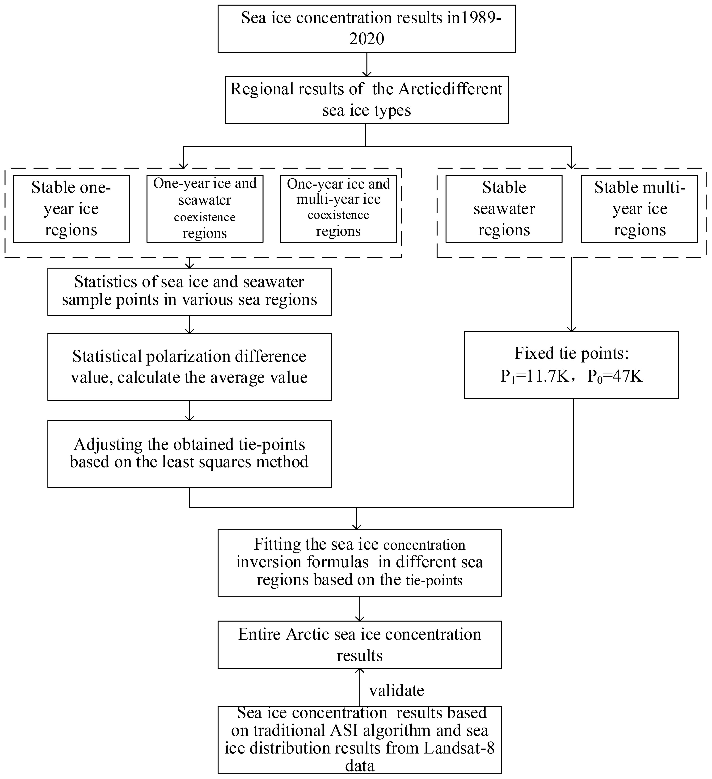
Figure 1 Flow chart of SIC inversion algorithm based on different sea ice regions.

3.2.1 Distribution results of the Arctic different sea ice regions

According to the sea ice seasonal variation, polar sea ice can usually be divided into one-year ice and multi-year ice (Massom and Comiso, 1994). The main difference between one-year ice and multi-year ice is the sea ice desalination during melting period in summer, resulting in lower salinity of one-year ice. Compared to one-year ice, multi-year ice is more prone to deformation, higher surface roughness, and thicker snow cover. In addition, due to one-year ice melting in summer and other processes, its surface is more uneven and more sensitive to microwave scattering (Perovich et al., 2002). These different features mean that their performance in microwave radiometer data will also vary. Different sea ice types have a significant impact on the energy exchange between the sea ice surface and the atmosphere. Therefore, accurate classification of different sea ice types is crucial.

The NASA Team SIC data is the most widely used dataset for calculating sea ice area and range (Cavalieri and Parkinson, 2012). Therefore, in this study uses the NASA Team SIC data from 1989 to 2020 as a reference, and obtains regional results for different sea ice types based on the sea ice melting duration. That is, we based on the daily average sea ice concentration data provided by NSIDC from 1989 to 2020, a 15% sea ice concentration threshold was used to distinguish the sea ice edge region. The overall Arctic sea ice distribution map was obtained for each year, and the entire Arctic region was divided based on the annual Arctic sea ice distribution map, combined with the average melting time of multi-year ice and one-year ice and their definitions. Finally, the Arctic is divided into stable one-year ice regions, one-year ice and seawater coexistence regions, one-year ice and multi-year ice coexistence regions, stable multi-year ice regions, and stable seawater regions. The results of regional division are shown in Figure 2.

Figure 2

Figure 2 Distribution results of different Arctic sea ice types.

Due to the fact that the distribution results of different sea ice types are obtained through the NASA Team algorithm, which is a low-frequency algorithm and uses data with different spatial resolutions compared to the ASI algorithm. In order to further ensure the inversion results accuracy for various sea ice types, polar stereo projection is performed on the distribution results of sea ice types, and bilinear interpolation method is used to resample them. The sea ice type distribution data is mapped to the same grid as the data used by the ASI algorithm, so that they have matching spatial resolution.

3.2.2 Tie-points

According to Wang’s study in 2009 on the polarization differences between one-year ice and multi-year ice brightness temperatures, it was found that with the arrival of summer, the brightness temperature of one-year ice gradually decreases and the polarization differences gradually increase (Wang, 2009). From July to October, the trend of one-year ice brightness temperature changes is almost consistent with that of open water. During this period, the one-year ice is in a melting state, and its surface brightness temperature characteristics are similar to open water.

Due to the fact that stable multi-year ice regions are year-round sea ice, and the sample points for obtaining sea ice tie-points in the ASI algorithm are selected as pure sea ice regions near the Canadian archipelago, which is a stable multi-year ice regions. The selection regions for sample points of seawater tie-points is in the south of the Greenland sea ice outer edge, which is a stable seawater regions with less seasonal variation than other sea regions. Therefore, the ASI algorithm is still used for SIC inversion in stable multi-year ice regions and stable seawater regions.

Based on the distribution maps of different sea ice types shown in Figure 2, the selection of sea ice and seawater sample points in the one-year and multi-year ice coexistence regions covers the entire year of 2021. For the selection of sea ice and seawater sample points in the stable one-year ice regions and the one-year ice and seawater coexistence regions, the selected time range is from January to June 2021 and from November to December 2021.

To ensure the representativeness of the selected sea ice and seawater sample points, the pixels that have been sea ice or seawater for 330 days are selected as sample points in the one-year ice and multi-year ice coexistence regions. Select the pixels with sea ice or seawater within 200 days as tie-points in the one-year ice and seawater coexistence regions and the stable multi-year ice regions, and calculate the polarization difference. By performing probability distribution statistics on the polarization difference calculated from daily sample points, the maximum probability value of polarization difference is selected as the polarization difference on the same day, and the average value within the selected days is calculated as the sea ice tie-points P1 and the seawater tie-points P0 for each region (as shown in Figures 3–5).

Figure 3

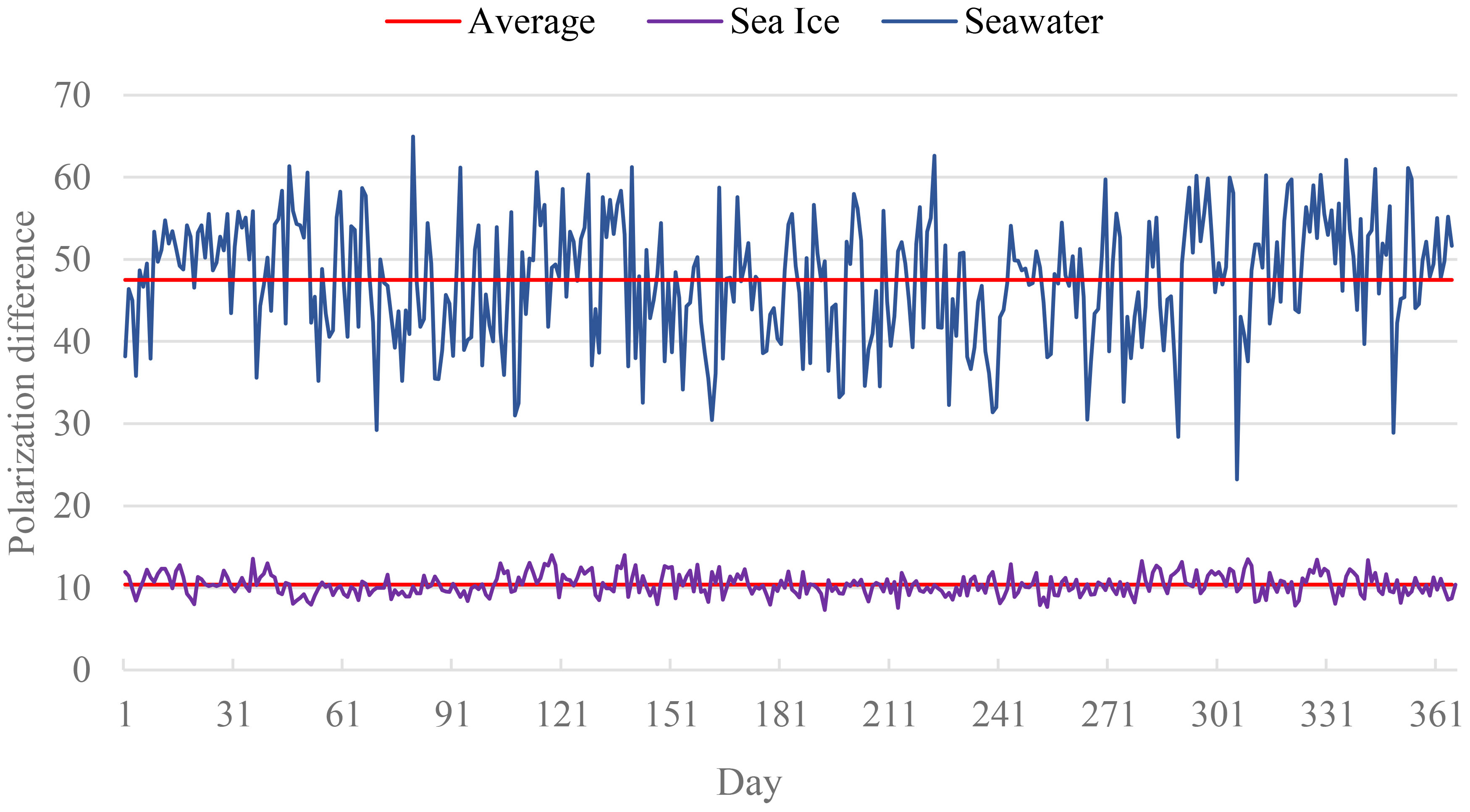
Figure 3 Stable one-year ice regions.

Figure 4

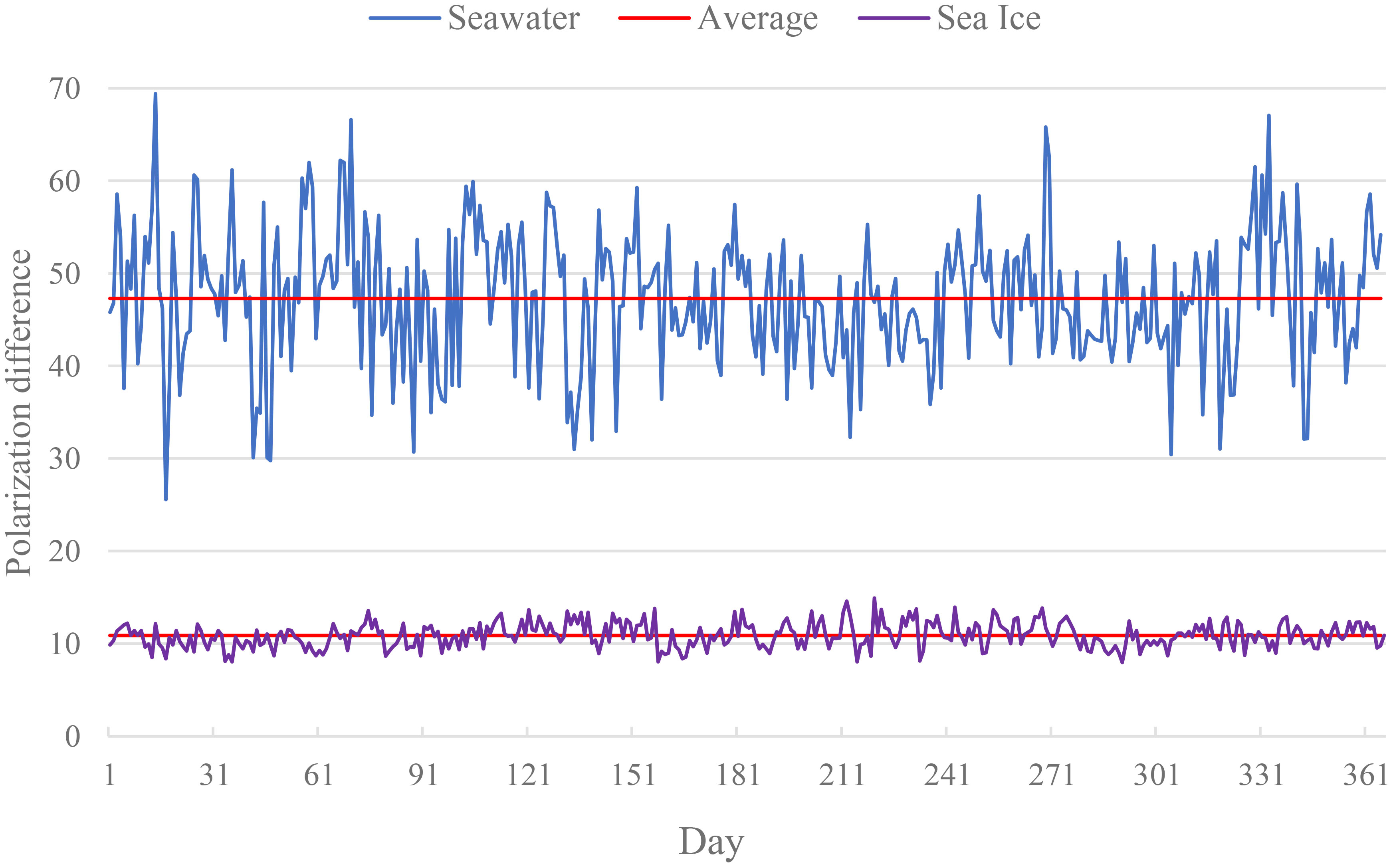
Figure 4 One and multi-year ice coexistence regions.

Figure 5

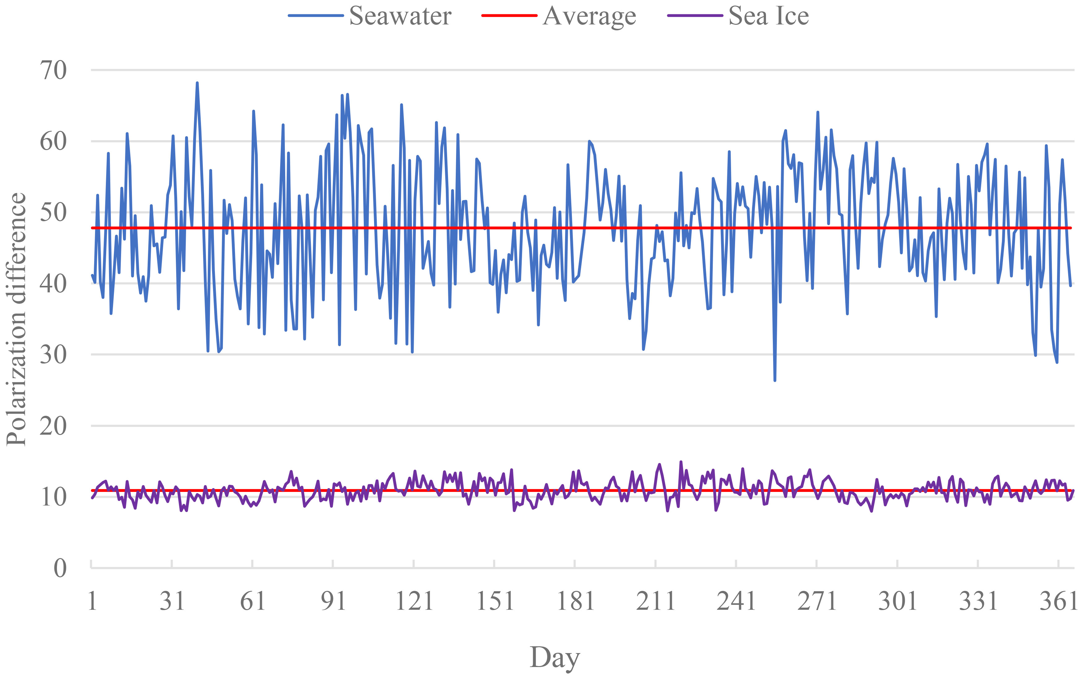
Figure 5 One -year ice and seawater coexistence regions.

According to the statistical results, the tie-points of the seawater in the stable one-year ice regions is P₀, which is 47.2K, and the tie-points of the sea ice is P₁, which is 11.5K. The seawater tie-points in the one-year ice and multi-year ice coexistence regions is 47.7K, and the tie-points of the sea ice is 10.8K. The tie-points of the seawater in the one-year ice and seawater coexistence regions is P₀, which is 47.5K, and the tie-points of the sea ice is P₁, which is 10.9K. The polarization difference of the one-year ice is mostly concentrated between 9K and 16K, while the polarization difference of sea ice in the multi-year ice and one-year ice coexistence regions is mostly concentrated between 8K and 14K, and the polarization difference of seawater is mostly concentrated between 30K and 68K. In addition, the polarization difference of the one-year ice brightness temperature in June is greater than in other months.

By utilizing the SIC data from the National Snow and Ice Data Center (NSIDC), we can further obtain accurate sea ice and seawater tie-points. The specific operation process is as follows that (1) Using polar stereo projection and grid interpolation methods, map the reference SIC and the SIC results obtained using the ASI algorithm on the same grid to minimize the least squares regression error. (2) Calculate the fitting parameters (slope and intercept) of least squares method between the reference SIC results and the SIC results obtained by the ASI algorithm. When the slope approaches 1 and the intercept approaches 0, obtain the final tie-points P₀ and P₁. Otherwise, adjust the tie-points and recalculate the slope and intercept. (3) In the stable one-year ice regions, the sea water tie-points P₀ is 47.4K, and the sea ice tie-points P₁ is 11.4K. In the one-year ice and multi-year ice coexist regions, the sea water tie-points P₀ is 47.7K, and the sea ice tie-points P₁ is 10.8K. In the one-year ice and water coexistence regions, the sea water tie-points P₀ is 47.6K, and the sea ice pixel value P₁ is 11K.

3.2.3 SIC inversion formulas in different sea ice regions

Calculate the polarization difference P of the brightness temperature based on the 89 GHz vertical polarization brightness temperature and horizontal polarization brightness temperature. Use a cubic polynomial to fit the SIC inversion formulas, and calculate the coefficients d₀, d₁, d₂, and d₃ shown in Table 1.

Table 1

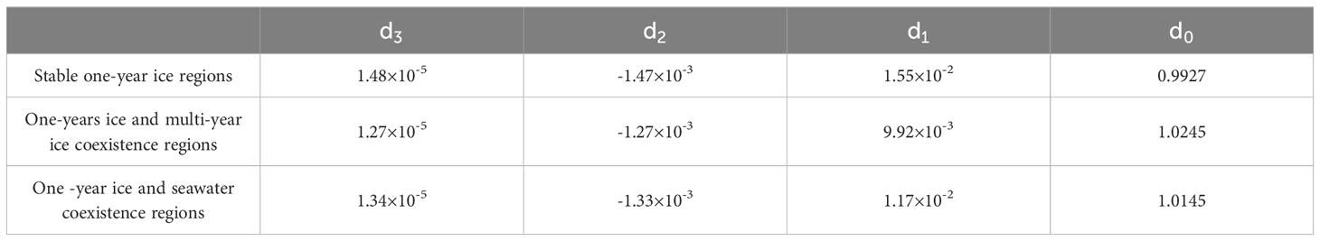
Table 1 Coefficients of different sea ice regions.

According to the results of the coefficients d₀, d₁, d₂, and d₃, the SIC inversion formulas can be fitted. The SIC inversion formula in the stable one-year ice regions is (Equation 3):

$\begin{array}{ll}\text{C}=1.48\times {10}^{-5}{\text{P}}^3-1.47\times {10}^{-3}{\text{P}}^2+1.55\times {10}^{-2}\text{P}+0.9927& (3)\end{array}$

The SIC inversion formula in the one-year ice and multi-year ice coexistence regions is (Equation 4):

$\begin{array}{ll}\text{C}=1.27\times {10}^{-5}{\text{P}}^3-1.27\times {10}^{-3}{\text{P}}^2+9.92\times {10}^{-3}\text{P}+1.0245& (4)\end{array}$

The SIC inversion formula in the one-year ice and seawater coexistence regions is (Equation 5):

$\begin{array}{ll}\text{C}=1.34\times {10}^{-5}{\text{P}}^3-1.33\times {10}^{-3}{\text{P}}^2+1.17\times {10}^{-2}\text{P}+1.0145& (5)\end{array}$

3.2.4 Inversion of Arctic SIC

Using different SIC inversion formulas in different sea ice regions, calculate their SIC, and combine them to obtain the entire Arctic SIC results. Verify spatial consistency by comparing the SIC results obtained from the traditional ASI algorithms, and local validation was performed using the sea ice distribution obtained from Landsat-8 data.

4 Results and validation

The winter in the Arctic regions lasts for six months, from November to April of the following year. The spring and autumn are from May to June and from September to October, respectively, while summer only includes July and August. Therefore, in this study selected four dates (February 15, May 15, July 15, and November 15, 2021) to obtain the ASI algorithm SIC results and the ASI SIC inversion algorithm results based on different sea ice regions for spatial consistency verification as shown in Figures 6–9.

Figure 6

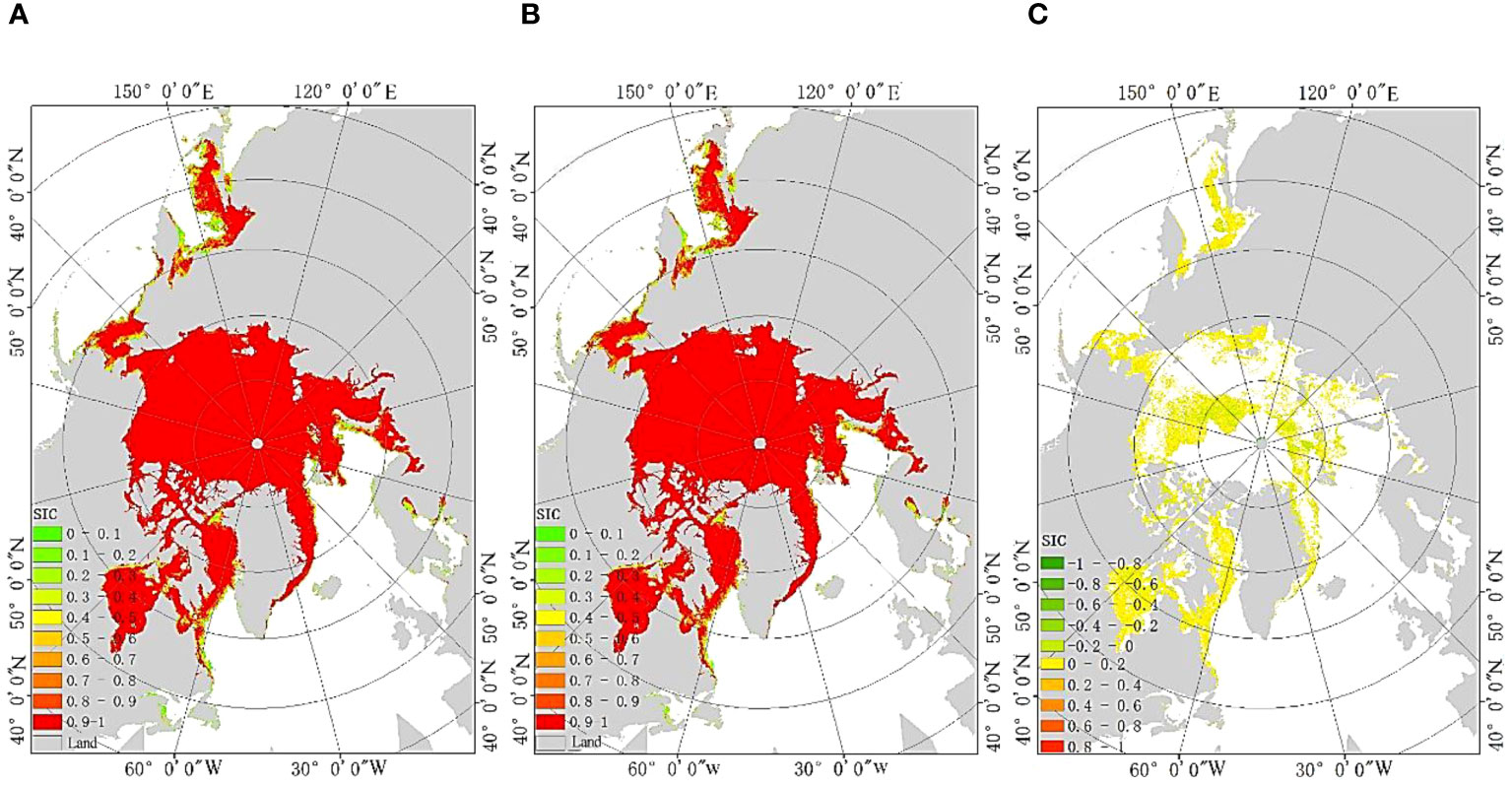
Figure 6 SIC results on February 15, 2021 (A) Traditional ASI algorithm (B) The proposed algorithm (C) Different regions between the two algorithms.

Figure 7

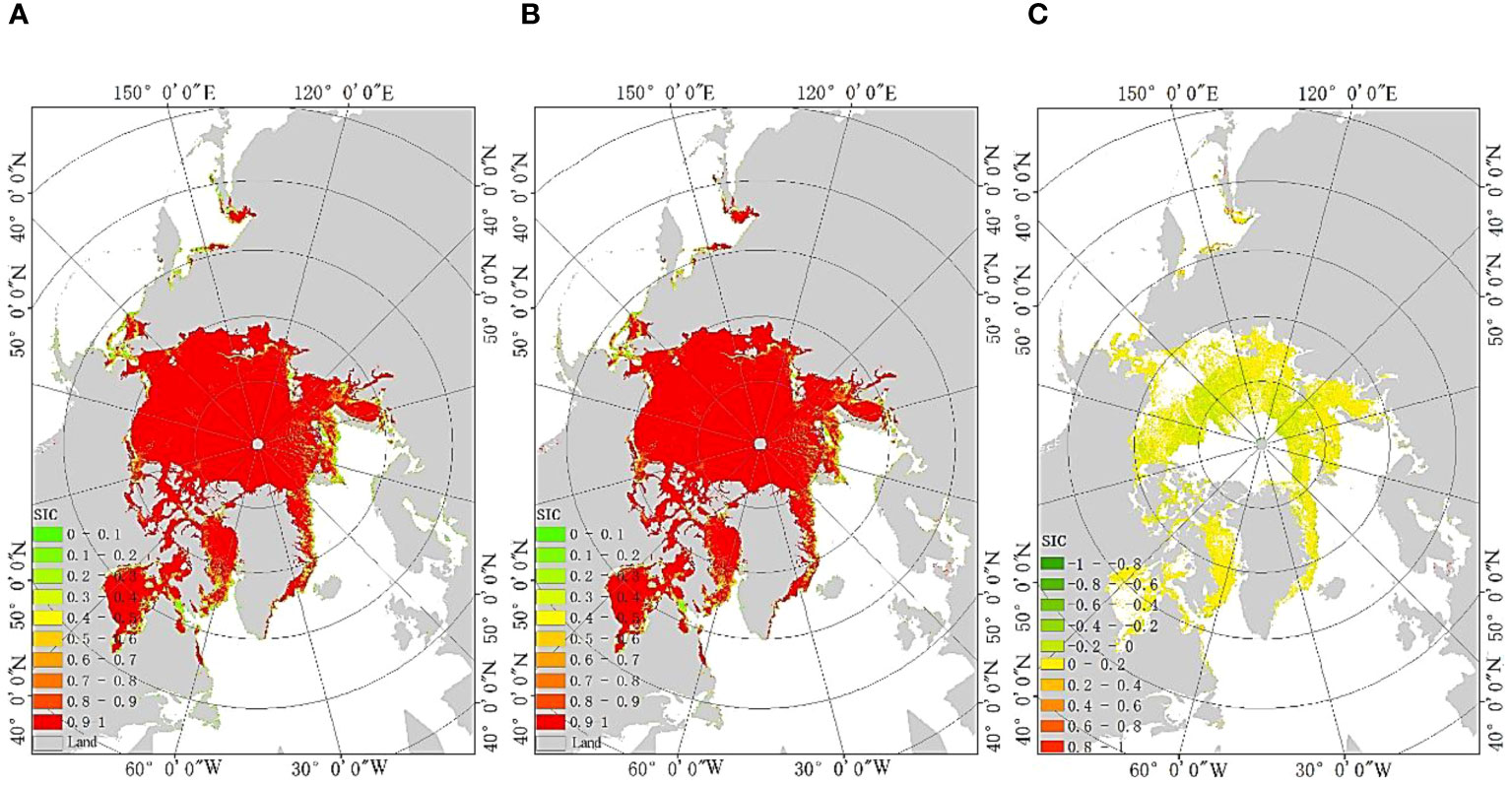
Figure 7 SIC results on May 15, 2021 (A) Traditional ASI algorithm (B) The proposed algorithm (C) Different regions between the two algorithms.

Figure 8

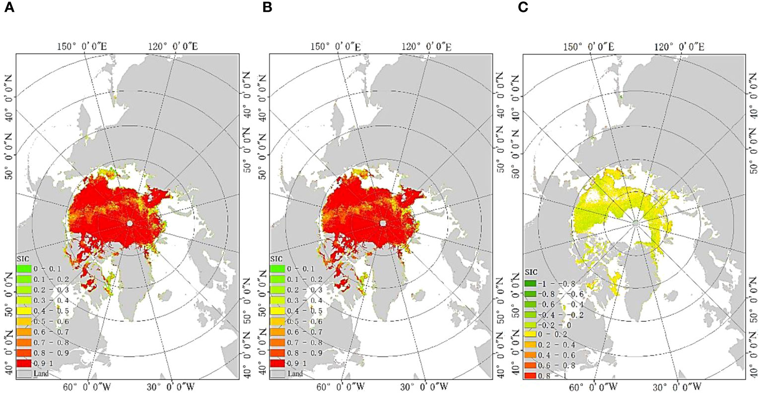
Figure 8 SIC results on July 15, 2021 (A) Traditional ASI algorithm (B) The proposed algorithm (C) Different regions between the two algorithms.

Figure 9

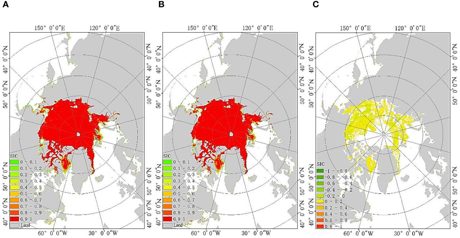
Figure 9 SIC results on November 15, 2021 (A) Traditional ASI algorithm (B) The proposed algorithm (C) Different regions between the two algorithms.

From the comparison results in Figures 6–9, it can be seen that the spatial distribution of SIC results between the ASI algorithm and the proposed algorithm is basically consistent. However, there are differences in the stable one-year ice regions, the one-year ice and multi-year ice coexistence regions, and the one-year ice and seawater coexistence regions, with SIC ranging from -0.027 to 0.058. In order to further validate the algorithm proposed in this study, the data from the 15th day of each month in 2021 were selected to compare the total sea ice area and daily average SIC results obtained by the proposed algorithm and the ASI algorithm. The comparison results are shown in Table 2.

Table 2

Table 2 Comparison of total sea ice area and daily average SIC between ASI algorithm and the proposed algorithm.

According to Table 2, there is not much difference between the ASI algorithm and the proposed algorithm in terms of total sea ice areas and daily average SIC. In addition, the algorithm proposed in this study has slightly higher results than the ASI algorithm in terms of total sea ice areas and daily average SIC.

To further validate, in this study compared the sea ice distribution results based on Landsat-8 data in May, July, and August 2021 with the sea ice distribution results of the ASI algorithm and the proposed algorithm. Due to the use of the same SIC inversion formulas as the ASI algorithm in both the multi-year ice regions and seawater regions, the validation regions mainly focuses on the stable one-year ice regions, one-year ice and multi-year ice coexistence regions, and one-year ice and seawater coexistence regions. For Landsat8 data, this study used the Normalized Difference Snow Index (NDSI) to detect sea ice. The calculation formula for NDSI is as follows (Equation 6):

$\begin{array}{ll}\text{NDSI}=(\text{R}1-\text{R}2)/(\text{R}1+\text{R}2)& (6)\end{array}$

Where R1 is the visible light channel reflectance (such as 0.55 μm, 0.67 μm, or 0.86 μm), and R2 is the shortwave infrared channel reflectance (such as 1.6 μm or 2.2 μm). During the day, if the defined solar zenith angle is below 85°, and the NDSI value is greater than 0.45 and the reflectance at 0.86 μm is higher than 0.08, it is considered to be covered by ice (Riggs et al., 1999). For Landsat-8 high-resolution optical remote sensing data, when the NDSI values calculated for the 5th and 6th bands are greater than 0.45 and the reflectance at 0.86 μm in the 5th band is greater than 0.08, the pixel is determined to be covered by sea ice.

In this study, 0.86 μm and 1.6 μm were selected as R1 and R2 channels. This is because for water bodies with high green pigment content, the NDSI value calculated for reflectance in the 0.55 μm wavelength band is too high, which may lead to misjudgment of snow/sea ice. However, the NDSI value calculated for reflectance in the 0.86 μm wavelength band does not exhibit this situation.

The local verification results of the one-year ice and multi-year ice coexistence regions are shown in Figure 10. The local verification results of the stable one-year ice regions are shown in Figure 11. Due to the fact that most of the regions where one-year ice and seawater coexistence regions in July and August are seawater, the validation of the regions was conducted in May, as shown in Figure 12.

Figure 10

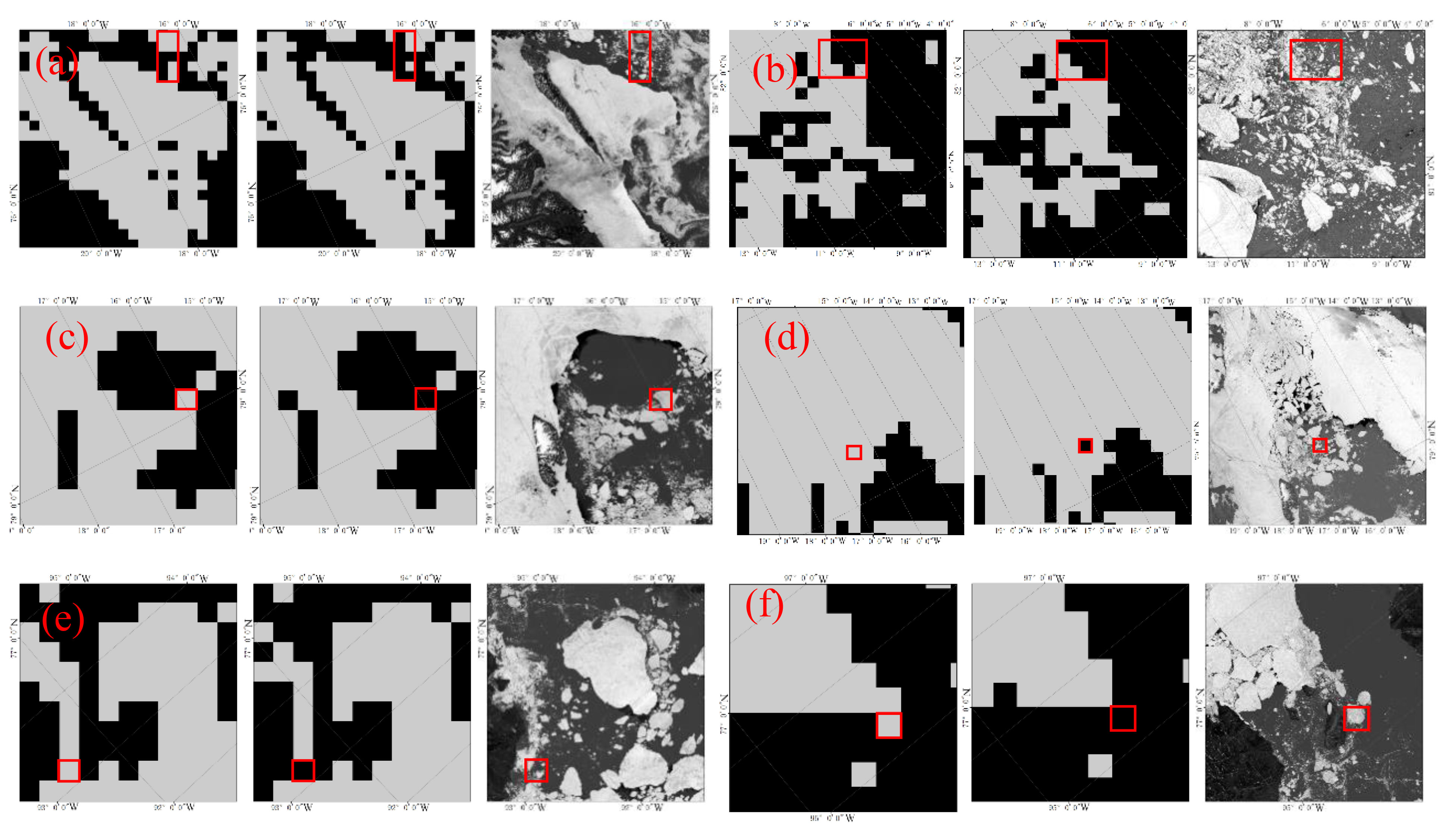
Figure 10 Local verification results of the one-year ice and multi-year ice coexistence regions based on sea ice distribution. (A) July 2, 2021, (B) July 6, 2021, (C) July 10, 2021, (D) July 20,2021, (E, F) August 6, 2021 (In panels (A-F), from left to right are that the proposed algorithm, the ASI algorithm, Landsat-8 data).

Figure 11

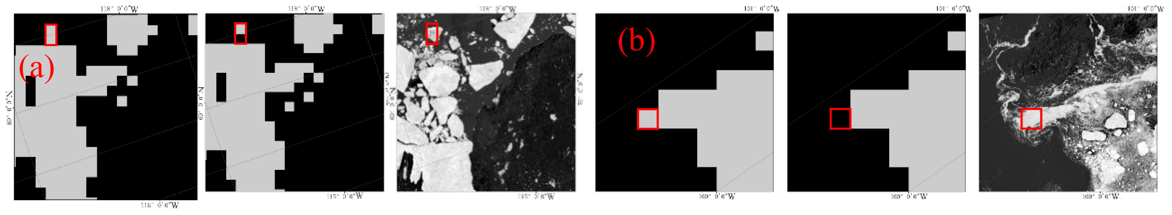
Figure 11 Local verification results of the stable one-year ice regions based on sea ice distribution. (A) July 3, 2021 (B) August 23, 2021 (In panels (A, B) from left to right are that the proposed algorithm, the ASI algorithm, Landsat-8 data).

Figure 12

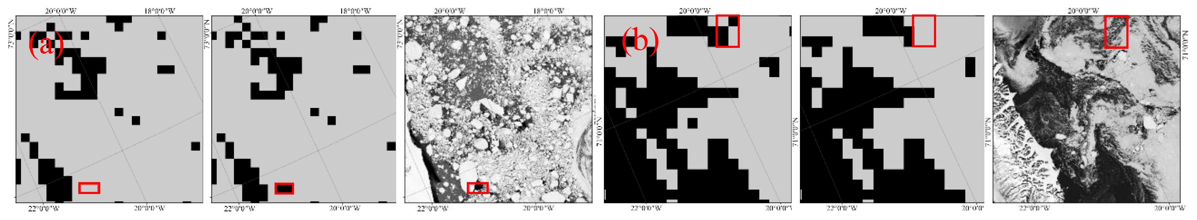
Figure 12 Local verification results of the one-year ice and seawater coexistence regions based on sea ice distribution. (A) May 19, 2021 (B) May 28, 2021 (In panels (A, B) from left to right are that the proposed algorithm, the ASI algorithm, Landsat-8 data).

From Figures 10–12, it can be seen that in the stable one-year ice regions, the one-year ice and multi-year ice coexistence regions, and the one-year ice and seawater coexistence, the results of the proposed algorithm based on different sea ice regions are closer to the sea ice results of Landsat-8 optical data. Based on the sea ice distribution results obtained from Landsat8 optical data, the accuracy of the sea ice distribution obtained from the proposed algorithm and ASI algorithm is shown in Table 3.

Table 3

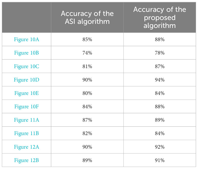
Table 3 Accuracy of sea ice distribution obtained from the proposed algorithm and ASI algorithm.

According to Table 3, the ASI SIC inversion algorithm based on different sea ice regions has significantly improved the accuracy of sea ice distribution compared to the ASI algorithm in the stable one-year ice regions, one-year ice and seawater coexistence regions, and one-year ice and multi-year ice coexistence regions. Compared with the ASI algorithm, the accuracy of the proposed algorithm has improved by a minimum of 2%, a maximum of 6%, and an average of 3.3%. Among them, the accuracy of the proposed algorithm has improved significantly in one-year ice and multi-year ice coexistence regions, with a rate of 4% -6%. In stable one-year ice regions and one-year ice and seawater coexistence regions, the accuracy of the proposed algorithm has improved by 2%.

5 Discussion

The ASI algorithm uses a unified sea ice and seawater tie-points to fit the SIC inversion formulas for different sea regions in polar regions. However, this method ignores the differences in the characteristics of different sea ice regions, such as significant differences in the thickness, structure, salinity, and radiation emissivity of sea ice between multi-year ice and one-year ice. Therefore, applying the same tie-points in different sea regions may lead to errors in the SIC inversion results, thereby reducing the inversion accuracy. If the different sample points are selected for the different sea ice regions to calculate the tie-points, the ASI algorithm can better capture the differences in characteristics of different sea ice types, thereby enabling the algorithm to more accurately invert SIC.

The algorithm in this study still uses the fixed tie-points obtained from the fixed tie-points method to invert SIC in the stable multi-year ice regions and the stable seawater regions, just like the ASI algorithm. In the stable one-year ice regions, one-year ice and seawater coexistence regions, one-year ice and multi-year ice coexistence regions, different from the fixed tie-points obtained from the ASI algorithm, the algorithm in this study selects the tie-points from these three regions and fits them to obtain for SIC inversion formulas. This makes the algorithm in this study more accurate and adaptable to complex sea ice environments than the ASI algorithm in the stable one-year ice regions, one-year ice and seawater coexistence regions, and one-year ice and multi-year ice coexistence regions.

However, there are still some shortcomings in this study that (1) There is a difference in the acquisition time between AMSR-2 data and Landsat-8 data, which may lead to errors in the sea ice distribution results obtained from the two types of data. Future study will consider incorporating radar data, higher resolution data, or site testing data to validate the algorithm proposed in this study. (2) Landsat8 data is susceptible to the interference of cloud and fog when selecting Landsat-8 data for local validation, current research only considers regions without cloud and fog interference, resulting in fewer local regions available for validation. Future study will consider cloud removal of Landsat8 data to more comprehensively validate the algorithm proposed in this study.

6 Conclusion

In this study addresses the issue of inaccurate inversion accuracy caused by the inability of the ASI algorithm to fully capture the differences between different sea regions and sea ice types when inverting polar SIC. An improved ASI SIC inversion algorithm based on different sea ice regions was proposed, and the SIC results in the Arctic regions were obtained. That is, according to the fitted inversion formulas, the corresponding SIC results are obtained in each region, and they are combined to obtain the total SIC result of the Arctic. Comparing the inversion results of the proposed algorithm with those of the ASI algorithm, it can be seen that the Arctic sea ice space obtained by the proposed algorithm is basically the same as that obtained by the ASI algorithm, and the total Arctic sea ice area and daily average SIC are not significantly different. However, the proposed algorithm is slightly higher than the ASI algorithm in terms of total sea ice area and daily average SIC. Moreover, in this study introduced Landsat8 data for cross validation, and the results show that the inversion accuracy of the proposed algorithm is 2% -6% higher than that of the ASI algorithm in the stable one-year ice regions, the one-year ice and multi-year ice coexisting regions, and the one-year ice and seawater coexisting regions.

Data availability statement

The datasets presented in this study can be found in online repositories. The names of the repository/repositories and accession number(s) can be found below: https://nsidc.org/data/NSIDC-0051.

Author contributions

XW: Conceptualization, Validation, Writing – review & editing. ZS: Conceptualization, Methodology, Supervision, Validation, Writing – original draft, Writing – review & editing. ZG: Methodology, Writing – original draft. YZ: Validation, Writing – original draft. YW: Validation, Writing – original draft.

Funding

The author(s) declare financial support was received for the research, authorship, and/or publication of this article. This research was supported by the Key Laboratory of Grain Information Processing and Control (Henan University of Technology), Ministry of Education (No. KFJJ-2020–113).

Conflict of interest

The authors declare that the research was conducted in the absence of any commercial or financial relationships that could be construed as a potential conflict of interest.

Publisher’s note

All claims expressed in this article are solely those of the authors and do not necessarily represent those of their affiliated organizations, or those of the publisher, the editors and the reviewers. Any product that may be evaluated in this article, or claim that may be made by its manufacturer, is not guaranteed or endorsed by the publisher.

References

Beitsch A., Kaleschke L., Kern S. (2014). Investigating high-resolution AMSR2 Sea ice concentrations during the February 2013 fracture event in the Beaufort Sea. Remote Sens. 6, 3841–3856. doi: 10.3390/rs6053841

CrossRef Full Text | Google Scholar

Cavalieri D. J., Gloersen P., Campbell W. J. (1984). Determination of sea ice parameters with the Nimbus 7 SMMR. J. Geophys. Res.: Atmos. 89, 5355–5369. doi: 10.1016/0198-0254(84)93205-9

CrossRef Full Text | Google Scholar

Cavalieri D. J., Parkinson C. L. (2012). Arctic sea ice variability and trends 1979-2010. Cryos. 6, 881–889. doi: 10.5194/tc-6-881-2012

CrossRef Full Text | Google Scholar

Comiso J. C. (2003). Large-scale characteristics and variability of the global sea ice cover. Sea ice: an introduct. to its phys. chem. Biol. geol., 112–142. ISBN:9780470757161. doi: 10.1002/9780470757161

CrossRef Full Text | Google Scholar

Feng T., Liu X., Li R. (2022). Super-resolution-aided sea ice concentration estimation from AMSR2 images by encoder-decoder networks with atrous convolution. IEEE J. Select. Topics Appl. Earth Observ. Remote Sens. 16, 962–973. doi: 10.1109/JSTARS.2022.3232533

CrossRef Full Text | Google Scholar

Gabarro C., Turiel A., Elosegui P., Pla-Resina J. A., Portabella M. (2017). New methodology to estimate Arctic sea ice concentration from SMOS combining brightness temperature differences in a maximum-likelihood estimator. Cryos. 11, 1987–2002. doi: 10.5194/tc-11-1987-2017

CrossRef Full Text | Google Scholar

Kern S. (2004). A new method for medium-resolution sea ice analysis using weather-influence corrected Special Sensor Microwave/Imager 85 GHz data. Int. J. Remote Sens. 25, 4555–4582. doi: 10.1080/01431160410001698898

CrossRef Full Text | Google Scholar

Ledley T. S. (1988). A coupled energy balance climate-sea ice model: Impact of sea ice and leads on climate. J. Geophys. Res.: Atmos. 93, 15919–15932. doi: 10.1029/JD093iD12p15919

CrossRef Full Text | Google Scholar

Lin H., Bao Q., Tian Z., Lin W., Xi L., Qun L. (2022). Comparison of remote sensing sea ice concentration products for Arctic shipping services. Polar Res. 34, 20–33. doi: 10.13679/j.jdyj.20210018

CrossRef Full Text | Google Scholar

Liu T. T., Liu Y. X., Huang X., Wang Z. M. (2015). Fully constrained least squares for antarctic sea ice concentration estimation utilizing passive microwave data. IEEE Geosci. Remote Sens. Lett. 12, 2291–2295. doi: 10.1109/LGRS.2015.2471849

CrossRef Full Text | Google Scholar

Liu Y., Key J., Mahoney R. (2016). Sea and freshwater ice concentration from VIIRS on Suomi NPP and the future JPSS satellites. Remote Sens. 8, 523. doi: 10.3390/rs8060523

CrossRef Full Text | Google Scholar

Lomax A. S., Lubin D., Whritner R. H. (1995). The potential for interpreting total and multiyear ice concentrations in SSM/I 85.5 GHz imagery. Remote Sens. Environ. 54, 13–26. doi: 10.1016/0034-4257(95)00082-C

CrossRef Full Text | Google Scholar

Markus T., Cavalieri D. J. (2000). An enhancement of the NASA Team sea ice algorithm. IEEE Trans. Geosci. Remote Sens. 38, 1387–1398. doi: 10.1109/36.843033

CrossRef Full Text | Google Scholar

Massom R., Comiso J. C. (1994). The classification of Arctic sea ice types and the determination of surface temperature using advanced very high resolution radiometer data. J. Geophys. Res.: Oceans 99, 5201–5218. doi: 10.1029/93JC03449

CrossRef Full Text | Google Scholar

Melsheimer C., Spreen G., Ye Y. F., Shokr M. (2023). First results of Antarctic sea ice type retrieval from active and passive microwave remote sensing data. Cryos. 17, 105–126. doi: 10.5194/tc-17-105-2023

CrossRef Full Text | Google Scholar

Parkinson C. L. (1987). Arctic sea ice 1973-1976: Satellite passive-microwave observations. Sci. Tech. Inf. Branch Natl. Aeronautics Space Admin. 490.

Google Scholar

Perovich D. K., Grenfell T. C., Light B., Hobbs P. V. (2002). Seasonal evolution of the albedo of multiyear Arctic sea ice. J. Geophys. Res.: Oceans 107, SHE 20–1-SHE 20-13. doi: 10.1029/2000JC000438

CrossRef Full Text | Google Scholar

Quan S., Weiguo G. (2011). Analysis of meteorological characteristics in the Arctic Ocean region. Navig. Technol. 05), 12–14.

Google Scholar

Riggs G. A., Hall D. K., Ackerman S. A. (1999). Sea ice extent and classification mappingwith the Moderate Resolution Imaging Spectroradiometer Airborne Simulator. Remote Sens. Environ. 68, 152–163. doi: 10.1016/S0034-4257(98)00107-2

CrossRef Full Text | Google Scholar

Shuang L. (2022). Research on polar sea ice concentration and thickness retrieval using remote sensing observations. Univ. Chin. Acad. Sci.

Google Scholar

Shugang Z., Jiangping Z., Min L., Shixuan L., Shuwei Z. (2018). An improved dual-polarized ratio algorithm for sea ice concentration retrieval from passive microwave satellite data and inter-comparison with ASI, ABA and NT2. J. Oceanol. Limnol. 36, 1494–1508. doi: 10.1007/s00343-018-7077-x

CrossRef Full Text | Google Scholar

Spreen G., Kaleschke L., Heygster G. (2008). Sea ice remote sensing using AMSR-E 89-GHz channels. J. Geophys. Res.: Oceans 113 (C2). doi: 10.1029/2005JC003384

CrossRef Full Text | Google Scholar

Svendsen E., Kloster K., Farrelly B., Johannessen O. M., Johannessen A., Campbell W. J., et al. (1983). Norwegian remote sensing experiment: Evaluation of the Nimbus 7 scanning multichannel microwave radiometer for sea ice research. J. Geophys. Res.: Oceans 88, 2781–2791. doi: 10.1029/JC088iC05p02781

CrossRef Full Text | Google Scholar

Svendsen E., Matzler C., Grenfell T. C. (1987). A model for retrieving total sea ice concentration from a spaceborne dual-polarized passive microwave instrument operating near 90 GHz. Int. J. Remote Sens. 8, 1479–1487. doi: 10.1080/01431168708954790

CrossRef Full Text | Google Scholar

Tikhonov V. V., Repina I. A., Raev M. D., Sharkov E. A., Ivanov V. V., Boyarskii D. A., et al. (2015). A physical algorithm to measure sea ice concentration from passive microwave remote sensing data. Adv. Space Res. 56, 1578–1589. doi: 10.1016/j.asr.2015.07.009

CrossRef Full Text | Google Scholar

Wang H. (2009). Multi year ice retrieval using passive microwave remote sensing radiometer AMSR-E 89GHz data. Ocean Univ. China.

Google Scholar

Wu Z., Wang X., Wang X. (2019). An improved ARTSIST sea ice algorithm based on 19 GHz modified 91 GHz. Acta Oceanol. Sin. 38, 93–99. doi: 10.1007/s13131-019-1482-7

CrossRef Full Text | Google Scholar

Xi Z., Ying C., Stefan K., Meng Q., Qing J., Pei F., et al. (2021). Sea ice concentration derived from FY-3D MWRI and its accuracy assessment. IEEE Trans. Geosci. Remote Sens. 60, 1–18. doi: 10.1109/TGRS.2021.3063272

CrossRef Full Text | Google Scholar