 Pierre Veillard1*
 Pierre Prandi1
 Marie-Isabelle Pujol1*
 Jean-Alexis Daguzé1
 Fanny Piras1
 Gérald Dibarboure2
 Yannice Faugère3
- 1Environement Business Unit, Collecte Localisation Satellites, Ramonville Saint-Agne, France
- 2Direction des systèmes Orbitaux et des Applications (DOA), Centre National d'Etudes Spatiales, Toulouse, France
- 3Direction de la Stratégie (DS), Centre National d'Etudes Spatiales, Toulouse, France
Polar sea surface height observation by radar altimeters requires missions with high-latitude orbit and specific processing to observe the sea-ice-covered region within fractures in the ice. Here, we combine sea surface height estimates from different radar satellites over the ice-free and ice-covered polar oceans to create cross-calibrated along-tracks and gridded products over the Arctic Ocean (2011–2021) and the Southern Ocean (2013–2021). The sea surface height from our regional polar products is in great agreement with tide gauges and bottom pressure recorders at monthly timescales in seasonally to year-round ice-covered regions. Thanks to the use of several missions and the mapping strategy, our multi-mission products have a greater resolution than mono-mission products. Part of the sea level variability of the Arctic Ocean product is related to the Arctic Oscillation atmospheric circulation. At long term, the Arctic altimetry sea level is coherent with in-situ steric height evolution in the Beaufort gyre, and negative sea level trends over the 10-year period are observed in the East Siberian slope region, which may be related to the local freshwater decrease observed by other studies. Our regional polar sea level products are limited by current understanding of the sea-ice lead measurements, and homogenization of these polar products with global sea level products needs to be tackled.
1 Introduction
Polar oceans are severely impacted by climate change. The Arctic Ocean experiences higher warming than elsewhere (Rantanen et al., 2022). It is subject to the decrease of sea ice and the warming and freshening of its water (Timmermans and Marshall, 2020) with a global impact through its interactions with the Atlantic and Pacific oceans (Jones et al., 1998). The Southern Ocean has a great impact on the mass balance of the Antarctic Ice Sheet (Holland et al., 2020) and has a strong influence on global ocean circulation and climate (Rintoul, 2018). It is therefore crucial to monitor the polar oceans. However, there is a significant gap of ocean observations in the polar oceans compared with most areas of the global ocean (Smith et al., 2019). Satellites enable to observe the sea level from space, thus limiting the difficult implementation of in-situ measurements. Sea level observations from satellites have been continuously made since 1993 for the open ocean, providing crucial information on the variability of the ocean at different spatiotemporal scales. However, in the polar regions, satellite observations of the sea level are limited by the ice coverage. The satellite observations are only possible in cracks in the ice pack (sea-ice leads). The first sea level observations in the sea-ice leads were made (Peacock and Laxon, 2004), and some polar sea level maps emerged for the Arctic Ocean (Armitage et al., 2016; Rose et al., 2019; Doglioni et al., 2023; Lin et al., 2023) and the Southern Ocean (Armitage et al., 2018a; Dotto et al., 2018; Naveira Garabato et al., 2019). These datasets are based on sea level data from one satellite at a time with different time lapses. Rose et al.’s (2019) Arctic Ocean dataset starts in 1993, providing a long time series that can be analyzed at climate scales in terms of sea level trends (Ludwigsen et al., 2022). However, the datasets are provided at a monthly timescale and limited to hundreds of kilometers of resolutions due to the use of only one satellite and the smoothing applied for the mapping.
Benefiting from most of the satellites available, multi-mission sea level maps have been produced over 2016–2020 for the Arctic Ocean (Prandi et al., 2021) and Southern Ocean (Auger et al., 2022). Thanks to the improved altimetry coverage and mapping strategy, these products enable to map smaller scales. The current paper presents an extension of those datasets following the methodology of Prandi et al. (2021). Compared with Prandi et al. (2021), some updates are made concerning geophysical corrections (mean sea surface and ocean tide) and mapping and cross-calibration parameters, thus improving the dataset. Additionally, whereas the datasets presented by the previous authors only consisted in gridded product (also identified as level 4 product) merging of the measurement from the different altimeter mission processed, we complete here the new polar Arctic and Antarctic product line with the cross-calibrated along-track data (also identified as level 3 product).
Our regional polar products provide sea level anomaly, absolute dynamic topography, and associated geostrophic currents over 2013–2021 for the Southern Ocean and over 2011–2021 for the Arctic Ocean. The products cover latitudes from 50° to 88° benefiting from Cryosat-2 data, which is the first radar satellite to provide observations north of 81.5°N and up to 88°N, latitudes that are necessary to observe the Arctic Ocean where there are few other observations. These polar products aim to monitor the sea level in the rapidly changing polar regions at different time scales. The current experimental products aim to be implemented in the frame of the Copernicus Marine Service.
Our regional polar experimental products complement the DUACS (Data Unification and Altimeter Combination System) DT21 open ocean global product (Taburet et al., 2019; Faugère et al., 2022, available at doi.org/10.48670/moi-00146). The polar products differ from DUACS DT21 open ocean products in three points: first they are restricted to high latitude and consider the data on sea-ice leads. Second is because they do not use the same altimeter standards and geophysical corrections. The main differences are observed for the MSS (Mean Sea Surface) and tide corrections. These fields are updated for our regional polar products. Finally, the DUACS DT21 open ocean products benefit from global calibration methodology that is not possible for the regional polar products; this is discussed in Section 4. The paper is organized as follows. The data to produce and analyze the satellite sea level products are presented in Section 2. The methodology to produce the polar datasets is presented in Section 3. Comparison and validation of the datasets with other data is presented in Section 4. Uncertainties and future perspectives to these datasets are discussed in Section 5.
2 Data
2.1 Satellite data
Satellite data in the ice-covered region come from three altimetry missions: Cryosat-2, SARAL/AltiKa, and Sentinel-3A. Table 1 summarizes the characteristics of the different satellites and input products that are used. The satellite data are available over different periods, and Cryosat-2 provides the longest time series starting in 2011. To use most of the satellite coverage available in the polar regions, other altimeters included in the DUACS DT21 open ocean product are used to refine the maps on open ocean.
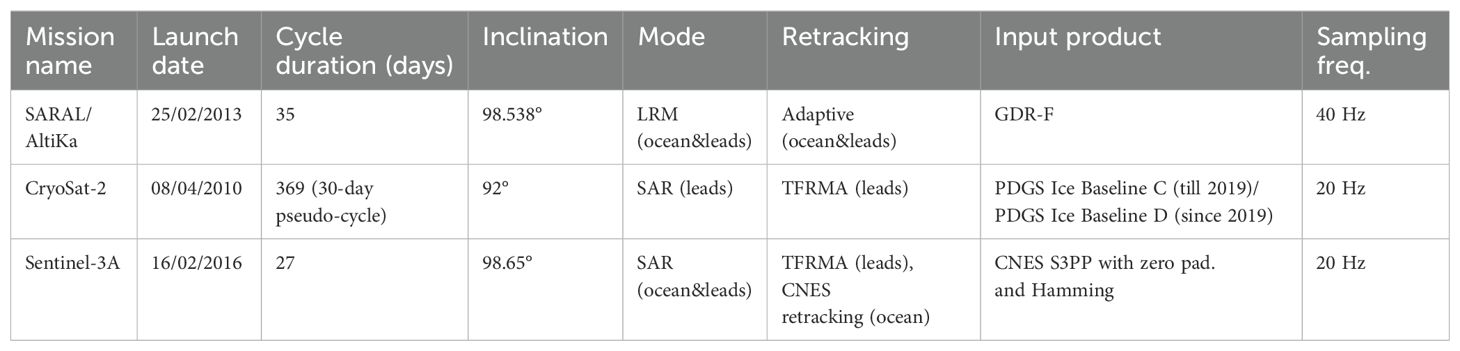
Table 1. Input data characteristics for each of the three altimetry missions.
A retracking step is necessary to estimate the range between the satellite and the ocean from the radar waveforms received by the satellite. Different retracking algorithms exist depending on the altimeter instrument onboard. SARAL/AltiKa operating in LRM (low-resolution mode) is processed using the Adaptive retracking (Poisson et al., 2018; Tourain et al., 2021). This retracking enables to process both specular echoes from the sea-ice leads and diffuse echoes from the open ocean, thus assuring a theorical continuity in range between the two surfaces, which is discussed in Section 5. Compared with empirical retracking, no bias is needed to be removed at the limit between the two regions, as done for other datasets (Armitage et al., 2016; Rose et al., 2019; Doglioni et al., 2023). For Cryosat-2 and Sentinel-3A satellites, the TFMRA (threshold first-maximum retracker algorithm) empirical retracking is used for specular echoes from the sea-ice leads. The combination between the different satellites is described in Section 3.2.
The sea surface height corresponds to the orbit of the satellite minus the estimated range. It is corrected from instrumental and geophysical corrections, and the MSS (Mean Sea Surface) is removed to get the SLA (Sea Level Anomaly) commonly used in ocean studies. The corrections applied are summarized in Table 2 For the most part, they are similar to the ones applied on open ocean. However, due to the ice-coverage, the application of some open ocean corrections may not be appropriate, and discussions are made here concerning three corrections. First, the sea-ice leads observations are not corrected for SSB (Sea State Bias) correction under the assumption that waves and winds are negligible in the ice-covered region and would not modify the estimated range, which is discussed in Section 5. Secondly, the wet troposphere correction accounting for wet troposphere radar delay comes from a model because radiometer estimates are not reliable on the sea-ice cover. It is applied to both open ocean and sea-ice leads data to assure continuity between the two surfaces (differences below 1 cm are found on open ocean between the correction from the model and the correction from the onboard radiometer). Thirdly, the dynamic atmospheric correction (DAC) is applied to remove both the large-scale effects of atmospheric pressure (inverted barometer (IB) formula) and the residual small-scale effects of wind forcing that are not resolved by altimetry (high-frequency component from a barotropic model following Carrère and Lyard, 2003). However, the latter barotropic model does not consider the ice cap feedback and it is not sure if it is valid to apply this component for the sea-ice leads observations. It is found that using the two components of the DAC rather than using only the IB component reduces the SLA variance (not shown). That should imply that correction errors are reduced by applying the two components. Doglioni et al. (2023) also noted improvements using the two components of the DAC on Cryosat-2 SLA in the Arctic region. It is therefore preferred to apply the two components of the DAC correction for both open ocean and sea-ice lead observations.
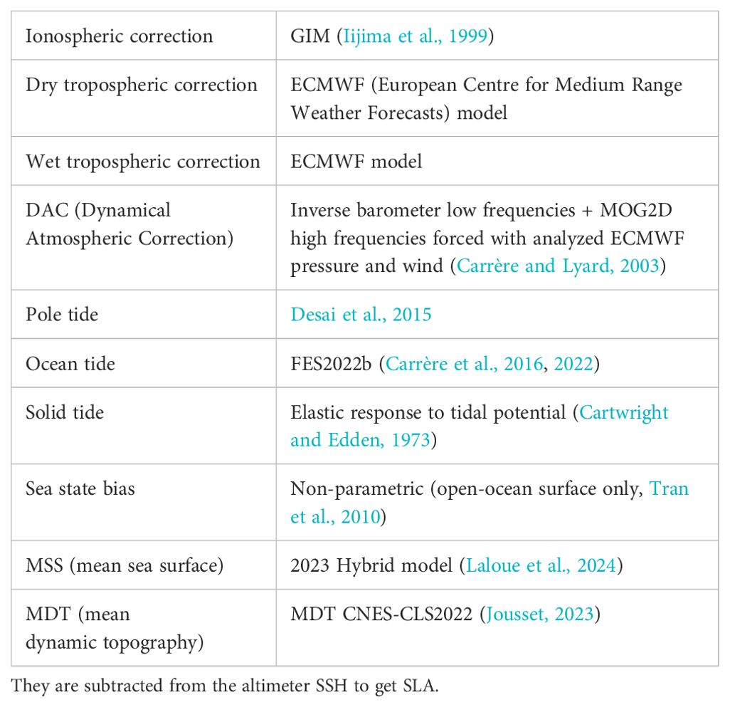
Table 2. Standards of the different corrections applied on altimeter measurements.
Other corrections are updated to new ones when possible. It concerns the use of the new FES2022 (Finite Element Solution, Carrere et al., 2022) tide correction improving the dataset especially in the Barents Sea (Supplementary Figure 1). The MSS is also updated to a new one (Laloue et al., 2024) combining 3 MSS to benefit from their individual added values. The ADT (absolute dynamic topography) field is computed by adding the MDT (mean dynamic topography) CNES/CLS22 (Jousset, 2023) to the SLA. However, the MSS used for MDT computation (MSS CNES/CLS22; Schaeffer et al., 2023) differs from the one used for the SLA computation (hybrid MSS; Laloue et al., 2024). This difference has large-scale impacts on the ADT field near the Canadian Arctic Archipelago; it needs to be corrected for the next version of our regional polar product by using more coherent MDT and MSS.
Two other defaults of homogeneity were identified on the input data and were empirically corrected. First, for Cryosat-2, two different input data are used depending on the period. The PDGS Ice Baseline C is used before 2019, and the PDGS Ice Baseline D (Payload Data Ground Segment) is used since 2019. A bias is added to the baseline C SLA by comparison with the baseline D SLA and to independent SARAL/AltiKa SLA (2.11 cm for the Arctic Ocean and 2.58 cm for the Southern Ocean) using gridded along-track data from the two satellites (see method in Section 3.2). Secondly, for open ocean measurements of SARAL/AltiKa, no SSB correction was available for the Adaptive retracking. Although the SSB correction is not necessary in lead areas (see discussion above), it remains essential in open ocean areas, especially since SARAL/AltiKa is subsequently used as a reference mission for the calibration of polar products (see Section 3.2). It is therefore important to correctly process the data over the open ocean for this mission. To this end, an SSB correction has been specifically defined. It was adapted from the MLE4 (maximum likelihood estimator) retracking with a correction depending on the SWH (Significant Wave Height) computed to minimize the difference between the MLE4 SLA and the Adaptive SLA. The linear correction depending on SWH (0.015*SWH for the Arctic Ocean and 0.01*SWH for the Southern Ocean) is added to the SSB correction. In addition, because of its smaller antenna aperture, SARAL/AltiKa’s Gaussian approximation of the antenna diagram, as modelized in the Adaptive retracker, is no longer valid for diffuse oceanic echoes that have a trailing edge driven by the antenna diagram (Jettou et al., 2023). Note that for peaky echoes, the shape is then driven by surface roughness (Tourain et al., 2021); therefore, this approximation has no impact on the range estimation and the retracker performs nominally. This SARAL/AltiKa specificity induces a dependence on SWH that is assumed to have a low impact on the estimated range after adapting the SSB correction.
2.2 Data for comparison
ICESat-2 is a laser altimeter that was launched in 2018 to observe frozen and icy areas. Compared with the radar altimetry missions described previously with observation footprints of several hundred of meters, ICESat-2 uses laser altimetry providing a reduced footprint up to 13 m that should improve the retrieval of sea-ice lead observations. ICESat-2 is equipped with six laser beams providing measurements up to 88°N. The first validation of the ICESat-2 sea level in the sea-ice leads were made by comparison with the conventional Cryosat-2 altimetry (Bagnardi et al., 2021). Here, we use the product ATL07 v5 (Kwok et al., 2021), providing ICESat-2 observations over the ice-covered region from October 2018 to June 2021. It provides SLA (variable “height_segment_height”) for the six beams; here, we only use beam 3 (spot 2R) as used in Bagnardi et al. (2021). Product corrections are already applied to the SLA, and we modify them to match the radar-altimeter corrections described in Table 1. However, it was not possible to modify the pole tide correction that is not available in the ICESat-2 product. Moreover, the atmospheric correction is from the ICESat-2 product because radar correction may not be appropriate for laser. The quality flag (variable “height_segment_quality”) and the sea-ice lead surface classification (variable “height_segment_ssh_flag” equals to 1) of the product are applied. Additional editing (sea ice concentration (SIC) threshold over 30%, |SLA|<2 m and large-scale outliers editing described in Section 3) is also used.
Other polar sea level maps from satellite altimetry are compared with the multi-mission maps produced. Extended versions of the datasets described in Armitage et al. (2016) for the Arctic Ocean and Armitage et al. (2018a) for the Southern Ocean are used (variable “DOT_smoothed” corresponding to smoothed ADT). Arctic ocean datasets from Rose et al. (2019) (variable “sea_level_anomaly”) and from Doglioni et al. (2023) (variable “sla”) are also used.
In-situ observations are scarce in the seasonally ice-covered polar oceans. Here, we select tide gauges (TG), bottom pressure recorders, and temperature/salinity profiles with data during the ice-covered season. TG data come from two databases with different resolutions. Gloss/Clivar provides hourly resolution time series (Caldwell et al., 2001) that are compared with altimetry at Prudhoe Bay TG on the Canadian coasts of the Beaufort Sea and Dumont D’Urville TG on the coast of Antarctica. The monthly PSMSL data (Holgate et al., 2013; PSMSL, 2024) provides more TG locations in the Arctic region, but they are of lower resolution. PSMSL TG trends are compared with altimetry sea level trends. To be comparable with altimetry sea level, the TG sea level is corrected from ocean tide, DAC, and glacial isostatic adjustment from model ICE5GVM4 (Peltier, 2004), accounting for the ongoing movement of land that is measured by tide gauges but not by altimetry.
Bottom pressure recorders (BPRs) measure the variations in ocean mass that are related to variations in sea level. Vinogradova et al. (2007) analyzed the relation between sea level and bottom pressure at different timescales. The study found that at high latitude (>60°), bottom pressure and sea level fields are essentially equivalent for periods up to around 100 days. We can therefore compare BPR variations with altimetry sea level at the intraseasonal timescale. To do so, BPR data are converted to sea level equivalent; the mean value is subtracted to consider an anomaly, and the time series are averaged daily to remove hourly variability that cannot be observed by altimetry. In the Arctic Ocean, we use the BPR A from the Beaufort Gyre Exploration Project (BGEP, https://www2.whoi.edu/site/beaufortgyre/) located in the Beaufort Sea and the BPR located near the North Pole that is under sea ice throughout the year (http://psc.apl.washington.edu/northpole/). In the Southern Ocean, the BPR ANT-17.1 from Androsov et al. (2020) is used.
The BGEP also provides temperature and salinity profiles at BPR A location that are used to estimate steric height to be compared with long-term sea level variations of the altimetry dataset. The temperature and salinity profiles for 2012–2022 are converted to steric height using the Thermodynamic Equation Of Seawater – 2010 with the gsw module in python (https://teos-10.github.io/GSW-Python/intro.html). The profiles sample different depths over the years, and the integration to get the steric height is made for depths from 70 m to 450 m to keep most of the profiles.
Arctic atmospheric circulation data are used to be linked with altimetry SLA variability. The daily Arctic Oscillation index (https://www.cpc.ncep.noaa.gov/products/precip/CWlink/daily_ao_index/ao.shtml) is used as regional index. It is averaged using a rolling window of 3 days and interpolated to the altimetry time of the grids (every 3 days). Similarly to Armitage et al. (2018b), seasonal and long-term signals are removed from the time series. More regionally in the Laptev Sea, the daily surface wind from NCEP/NCAR model reanalysis (https://psl.noaa.gov/data/gridded/data.ncep.reanalysis.html) is averaged using a rolling 15-day window and compared with altimetry sea level.
Monthly maps of Arctic melt pond fractions processed from satellite using MODerate resolution Imaging Spectroradiometer (Lee and Stroeve, 2021) are used to analyze defaults in the Arctic dataset during the summer period.
3 Method
The production of satellite altimetry cross-calibrated along-tracks and maps from mono-mission SLA is described in this section. It documents the editing, cross-calibration, and merging of the data. It follows the methodology described in Prandi et al. (2021) with some differences especially concerning the use of new parameters for the optimal interpolation and difference in calibrations between missions and with DUACS DT21 open ocean dataset.
3.1 Along-track editing
Editing is needed to select the data we want and discard outliers. First, sea-ice leads and open ocean observations are separated thanks to neural network classification of the satellite waveforms (Poisson et al., 2018). This process is combined with thresholds on SIC and satellite backscatter coefficients that are summarized in Table 3.
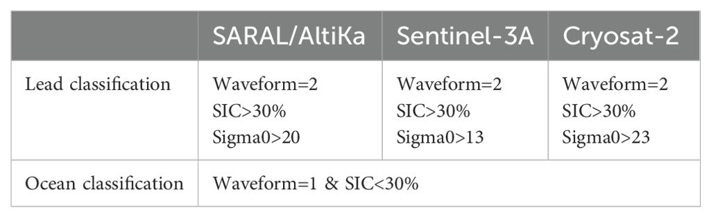
Table 3. Thresholds used to differentiate leads and open ocean observations.
Secondly, additional editing of the data is applied to SARAL/AltiKa considering its operating mode. The range estimation is influenced by small bright targets such as sea-ice leads in the radar footprint. Satellites may thus be “hooked” by the sea-ice leads and receive sea-ice leads echoes when they are not directly on-nadir. This phenomenon is referred to as “snagging” or “off-nadir hooking” (Quartly et al., 2019). SARAL/AltiKa operates in LRM mode with along-track and across-track footprints of approximately 1.64 km whereas the other satellites in SAR mode have an along-track footprint of 300 m. Therefore, for SARAL/AltiKa, the “off-nadir hooking” observations are more present in the along-track direction. An editing is therefore applied on SARAL/AltiKa to select the observations the more on-nadir of the sea-ice leads in the along-track direction corresponding to the maximum of the backscatter coefficient. The selection keeps the observations corresponding to the maximum of the backscatter coefficient on a rolling window of six observations. By applying this editing, off-nadir measurements corresponding to low SLA are removed, and on average, the sea-ice lead SLA is increased by 1.7 cm whereas the SLA gets lower near the open ocean region for unknown reasons (not shown). By applying this strategy, the SARAL/AltiKa SLA gets closer to Sentinel-3A SLA (Supplementary Figure 2). The selection on a 6-measurement rolling window reduces the 75-km/10-day box variance of difference of SLA between SARAL/AltiKa and Sentinel-3A by 5% whereas the SARAL/AltiKa 75-km/10-day coverage is reduced by 7% showing a good compromise.
Finally, additional editing (similar to Prandi et al., 2021) consists in removing outlier observations in three steps. First, observations with bad retracking fit are removed and absolute SLA over 2 m is removed. Then, an iterative editing is applied for open ocean observations similarly to DUACS processing. Finally, large-scale outlier observations exceeding 2.5 times the standard deviation of along-track SLA in 200-km/3-month boxes from the SLA mean are discarded. By applying the editing, we get along-track sea level observations that are similar between the missions, as presented in Section 4.1.
3.2 Along-track calibration
To compare inter-mission SLA differences between the different altimetry missions, the along-track SLA for each mission is averaged in boxes of 75 km/10 days and the difference between the two missions in each collocated box is computed. Then, the collocated boxes of difference can be averaged in time to get the map of inter-mission difference or averaged in space to get the time series of inter-mission difference. The inter-mission calibration is done by removing a bias and a seasonal signal. The inter-mission bias is computed as the median over all the collocated boxes of difference, and the seasonal signal as an annual seasonal fit on the time series of inter-mission SLA difference.
This method is used to calibrate Cryosat-2 and Sentinel-3A SLA on SARAL/AltiKa by correcting from the inter-mission bias plus an annual seasonal signal on both the open ocean and the sea-ice lead surfaces. The values of the corrections are summarized in Table 4. Additional calibration strategies for future datasets are discussed in Section 5.
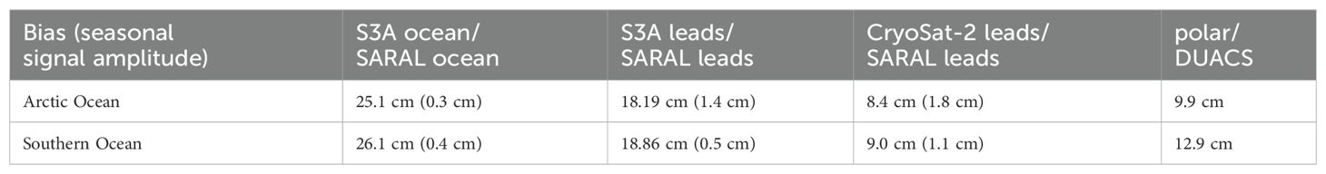
Table 4. Biases and seasonal signal amplitude used to calibrate missions on SARAL/AltiKa (first four columns) and bias estimated between our regional polar L4 maps and the DUACS DT21 open ocean maps (last column).
The calibration of the measurements from different missions is then completed to reduce the regional bias that can be observed between neighboring (in space and time) tracks (see Section 3.3) and to make the regional polar product consistent with the DUACS open ocean global product (see Section 3.4).
3.3 Combination of the missions
We get edited and calibrated along-track SLA for the three missions that are combined to produce our level-3 (L3, multi-mission cross-calibrated along-track) and level-4 (L4, multi-mission maps) regional polar products. To do so, we use the optimal interpolation (OI) scheme (Bretherton et al., 1976; Le Traon et al., 1998; Ducet et al., 2000) to reduce geographically correlated errors between the missions. The method relies on a priori knowledge of different parameters such as the signal variance, correlation scales, long-wavelength error, and measurement error. All these parameters were defined specifically for the polar oceans. For the Southern Ocean, the a priori parameters are similar to Auger et al. (2022). For the Arctic Ocean, the map of a priori parameters for the signal variance, the long-wavelength error, and the measurement error are updated compared with Prandi et al. (2021). Firstly, the a priori map of signal variance (Supplementary Figure 3) is computed as the variance of Prandi et al.’s (2021) dataset within spatiotemporal boxes of 100 km/10 days (approximately the correlation scales). It is higher in the areas of high variability such as the coastal regions where high variability occurs as well as in the Lofoten basin and gulf stream regions. Secondly, the a priori map of long-wavelength error is adjusted; it is used by OI to reduce the relative between-track biases in a given area at scales of around 300 km. Long-wavelength error maps (Supplementary Figure 4) are computed from the variance of the long-wavelength correction after one iteration of OI with in addition MSS and ionospheric errors, as done for DUACS processing. Finally, the a priori measurement error maps are computed by addition of some components to the instrumental noise. The instrumental noise for the lead observations (not shown) is computed for each satellite as the variance of the along-track data in boxes of 25 km/10 days assumed to contain no ocean signal, and the variance in the boxes is averaged over time to get the map. Additional terms, also introducing sea level biases between neighboring tracks, are also considered (part of the variance of the signal and MSS and wet tropospheric errors), as also done in the DUACS open ocean processing (Taburet et al., 2019, Faugère et al., 2022). The correlation scales correspond to the spatiotemporal radius considered to correlate the input data, and it is kept to DUACS values with correlation scales around 100 km/10 days in the Arctic Basin (not shown).
The OI scheme is applied to compute L4 SLA maps and cross-calibrated L3 SLA along-tracks. The L4 maps are given on an area equal EASE-grid 2.0 (Brodzik et al., 2012) with a resolution of 25 km/3 days since a regular grid in degrees would not be equal in area at high latitude (1° of longitude is equal to 11 km at 80°N whereas it is equal to 111 km at 0°N). The L3 along-track observations are filtered using a Lanczos filter (as done for DUACS) with one positive lobe with a half window of approximately 40 km. Although a filtering with negative lobes should produce a better frequency response, it is not used here because the sea-ice lead observations are sparsely sampled, and outliers are introduced if lots of observations are associated with the negative lobe weighting and few are associated with a positive lobe. Finally, the L3 along-track are subsampled to deliver a 5-Hz (~1-km) resolution product.
3.4 Calibration with the DUACS global open ocean product
The reference of SLA of our regional polar products is set to DUACS DT21 open ocean SLA reference by subtracting a constant bias (values in Table 4) that is computed between our regional polar sea level maps and DUACS DT21 sea level maps on the common open ocean region. In Section 5, discussions are made about the remaining differences between the two datasets and additional calibration that may be used for future regional polar datasets.
3.5 Comparison of measurements from different altimeter missions
To compare inter-mission SLA differences between the different altimetry missions, the along-track SLA is averaged in boxes of 75 km/10 days and the difference between collocated boxes from two missions are averaged spatially to get the map of inter-mission difference or in time to get the time series of inter-mission SLA difference.
3.6 Comparison with in-situ datasets
To be compared with in-situ observations, altimetry sea level maps are collocated at an in-situ position by selecting the nearest valid altimetry grid node to the in-situ location and the mean value from the time series are subtracted to compare the two datasets relatively. Comparisons are made at different timescales over and below 60 days. For a period over 60 days, the 60-day rolling mean signal is used, and for a period below 60 days, the 60-day rolling mean signal is removed from the time series.
4 Results
4.1 Inter-mission consistency and variance of the maps
The maps of inter-mission SLA differences in 75-km boxes for the sea-ice leads and open ocean surfaces are shown for the Arctic and Southern Ocean (Figure 1). Differences are below 4 cm over most of the regions, showing that the observations from the different missions are coherent. There are more differences between the missions at the limit between the open ocean and the ice-covered regions and in coastal regions where there is more uncertainty and fewer data for comparison.
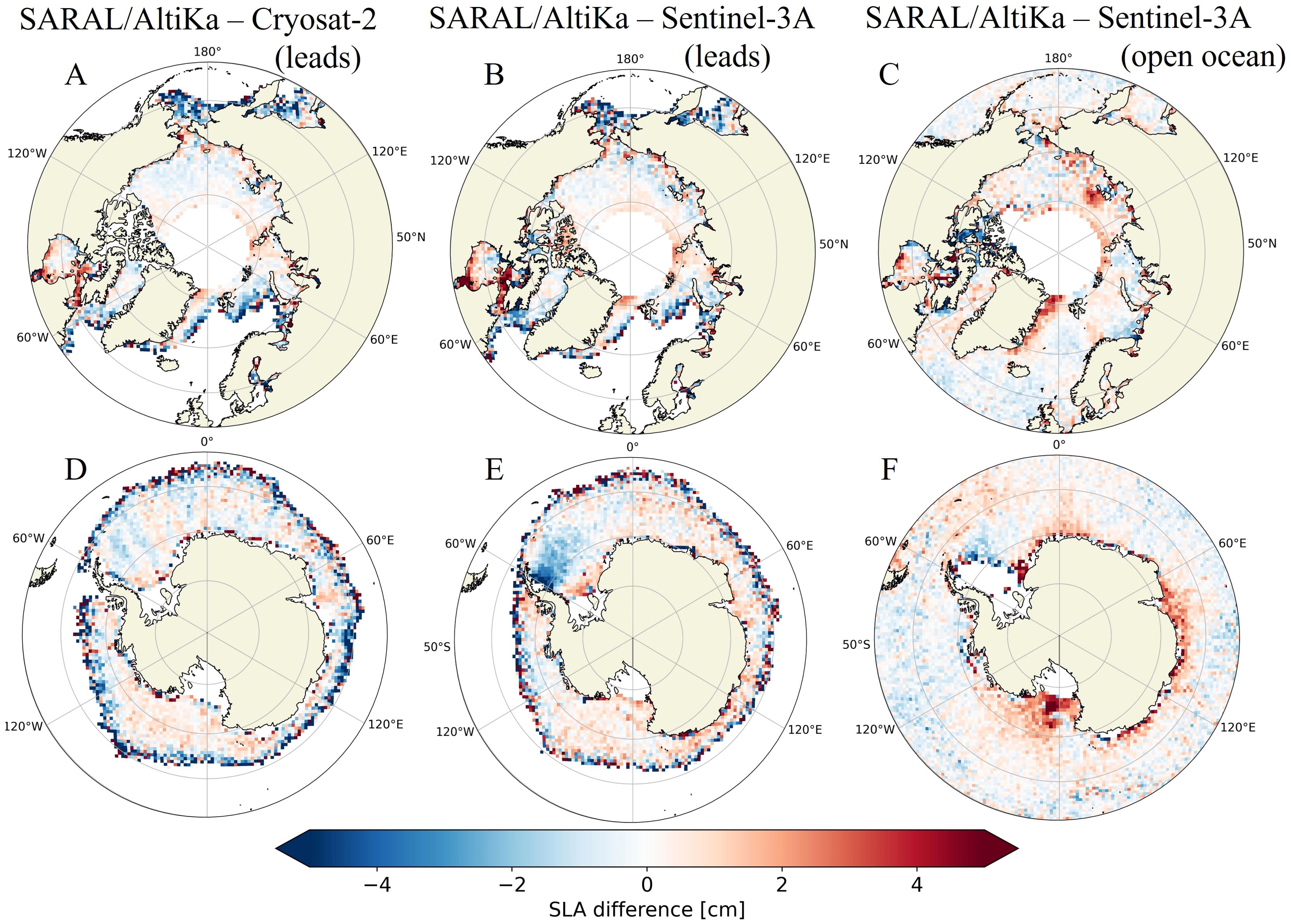
Figure 1. Inter-mission difference for the Arctic Ocean (A–C) and the Southern Ocean (D–F) as temporal mean of the SLA difference between the two missions in collocated 75-km/10-day boxes. The median difference between the two missions is removed.
The sea level temporal variance of our regional polar maps are plotted for the Arctic Ocean and for the Southern Ocean on Figure 2. They show large-scale features similar to the one observed with other altimetry datasets (Armitage et al., 2016; Rose et al., 2019; Doglioni et al., 2023; Armitage et al., 2018a). In the Arctic Ocean, coastal variability (Danielson et al., 2020) and Lofoten basin variability (Volkov et al., 2013) are visible.
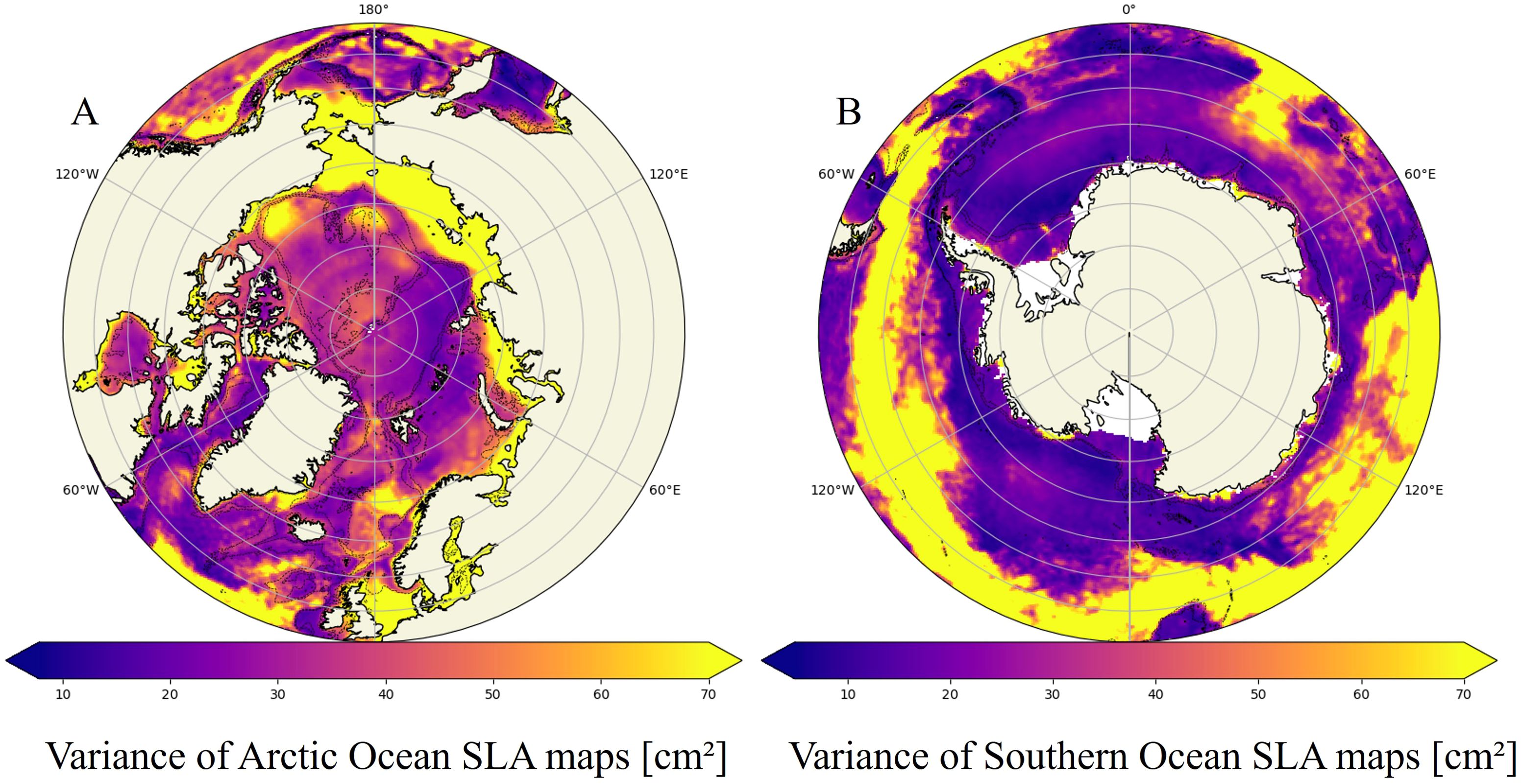
Figure 2. Arctic Ocean (A) and Southern Ocean (B) SLA variance of the maps. Black dotted lines denote bathymetry lines at 100 m, 1,000 m, and 2,000 m.
The variance are reduced compared with previous multi-mission datasets (Prandi et al., 2021 and Auger et al., 2022) in some areas. For the Arctic Ocean (Supplementary Figure 14), the variance is reduced in most of the region by using a new mapping parameter, especially the new a priori map of the signal variance in the OI scheme that was abnormally high in Prandi et al. (2021). Variance reduction in the North Atlantic Ocean and Barents Sea can be linked with improvement of the ocean tide correction in these regions. For the Southern Ocean (Supplementary Figure 15), the variance is reduced in part of the Weddell Sea with the new MSS and the overall variance reduction may be explained by new inter-mission calibration.
4.2 Comparison with ICESat-2 laser altimetry
Our radar altimeter measurements are compared with the ICESat-2 laser altimeter in the ice-covered region of the Arctic Ocean. The maps of difference in 75-km/10-day boxes in Figure 3 show that ICESat-2 sea-ice lead SLA is close to Cryosat-2, SARAL/AltiKa, and Sentinel-3A SLA with regional differences below 4 cm. Higher differences are present at the limit with the open ocean surfaces where there are few sea-ice lead measurements. Supplementary Figure 5 shows the evolution of the difference between ICESat-2 SLA and radar SLA over time. Unexplained differences are present at a yearly timescale. ICESat-2 left beam (2, 4, 6) and right beam (1, 3, 5) SLA evolutions differ at a yearly timescale (not shown), and the difference between the different beams should be analyzed in more detail. Supplementary Figure 6 presents the coverage in time and space provided by ICESat-2 compared with Cryosat-2. ICESat-2 observes 70% of the 75-km/10-day boxes that are observed by Cryosat-2. ICESat-2 coverage is especially reduced in winter. This difference of coverage may be due to the presence of clouds that prevent ICESat-2 observations as well as to too severe editing. In short, comparison of the radar altimeters with the ICESat-2 laser altimeter in the ice-covered region shows that using different instruments (laser and radar) associated with different retrackers, similar signals are observed in the sea-ice leads, thus validating the radar dataset. In the future, ICESat-2 observations in the ice-covered region may be used in combination with radar observations.
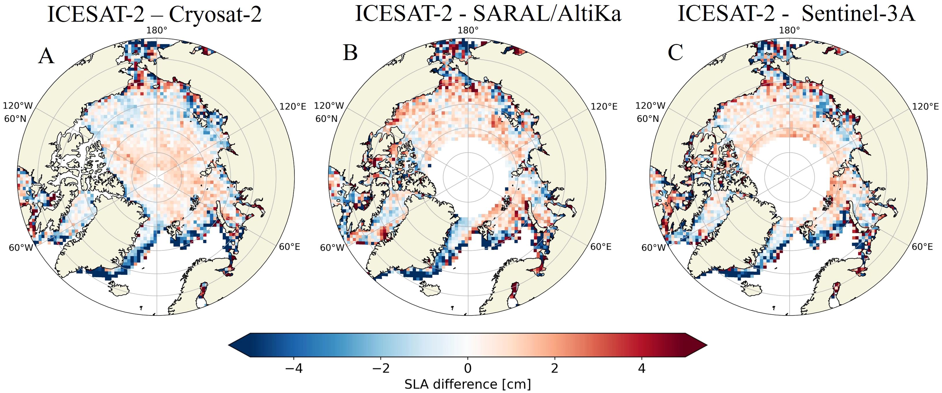
Figure 3. Map of difference of SLA between ICESat-2 and Cryosat-2 (A), SARAL/AltiKa (B), and Sentinel-3A (C) as temporal mean of SLA difference between the two missions in collocated in 75-km/10-day boxes. The median difference between the two missions is removed.
4.3 Comparison with in-situ sea level time series
Our regional polar sea level maps are compared with in-situ time series in the seasonally ice-covered region, and the correlation coefficient (Pearson’s) between the time series is computed at different timescales and summarized in Supplementary Table 1. The tide gauge (TG) sea level is corrected to observe similar signals as altimetry (Section 2.2) and compared with altimetry at short and long timescales. Compared with Prudhoe Bay TG, the Arctic altimetry SLA is well correlated including during the ice-covered period with an overall correlation of 0.65 (Figure 4). Time series from other mono-mission datasets (Armitage et al., 2016; Rose et al., 2019; Doglioni et al., 2023) are correlated at a seasonal timescale with TG time series, but shorter timescale variations are not depicted by these datasets. The correlation remains moderate for timescales below 60 days (removal of the 60-day rolling mean) with a correlation of 0.60. For timescales above 60 days (60-day rolling mean), the correlation is 0.71. As shown in Figure 5, similar comparisons are made with the Dumont D’Urville tide gauge with an overall correlation of 0.41 (0.21 for timescales below 60 days and 0.52 for timescales above 60 days). The lower correlation with Dumont D’Urville may be explained by the location of the tide gauge in a cove with local sea level variability.
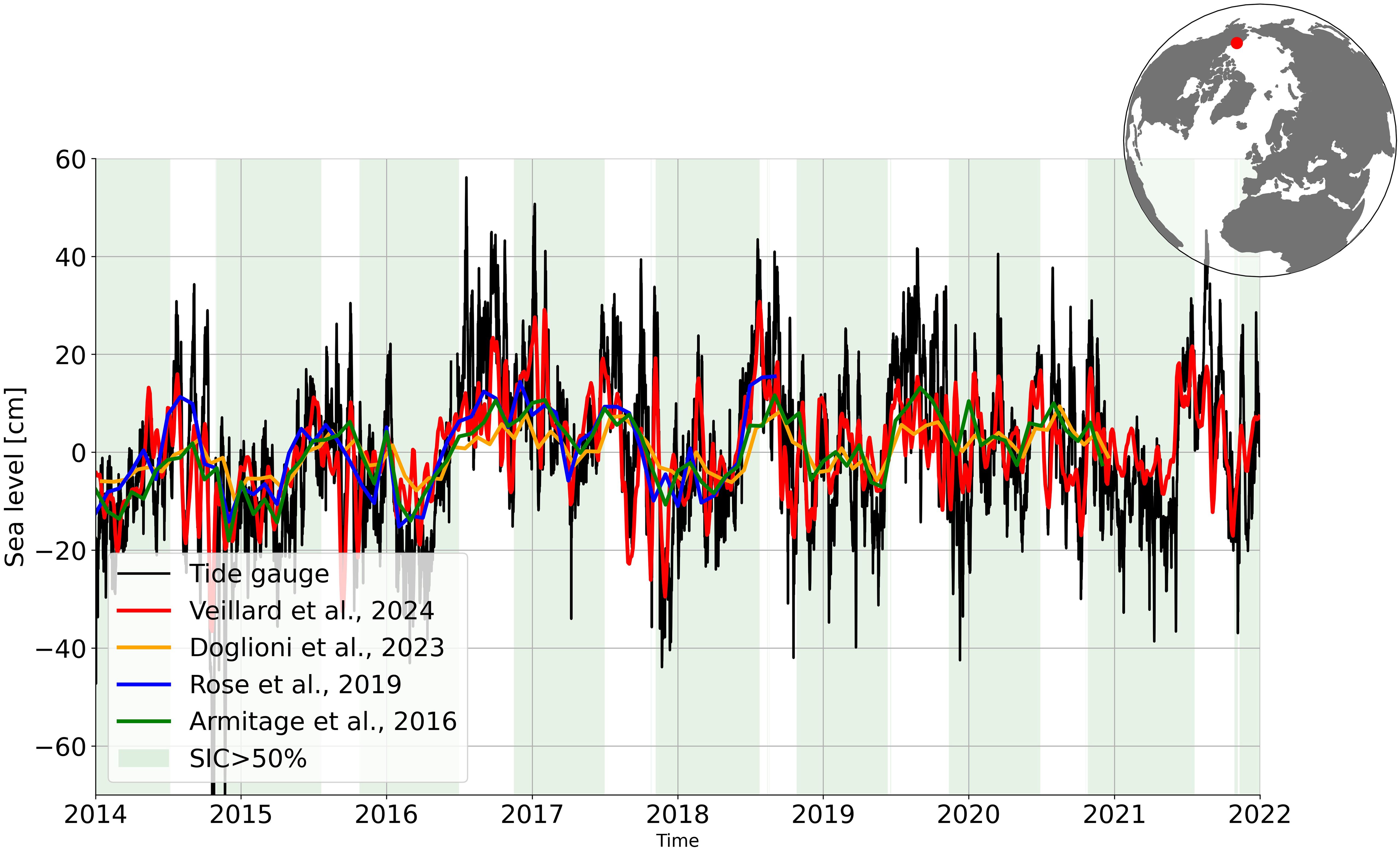
Figure 4. Arctic Ocean SLA maps from current paper (red) and Doglioni et al. (2023) (yellow) and Rose et al. (2019) (blue) and Armitage et al. (2016) (green) vs. Prudhoe Bay tide gauge (black). Green shades denote periods when the sea ice concentration is over 50%. Altimetry nearest grid node from the TG is selected.
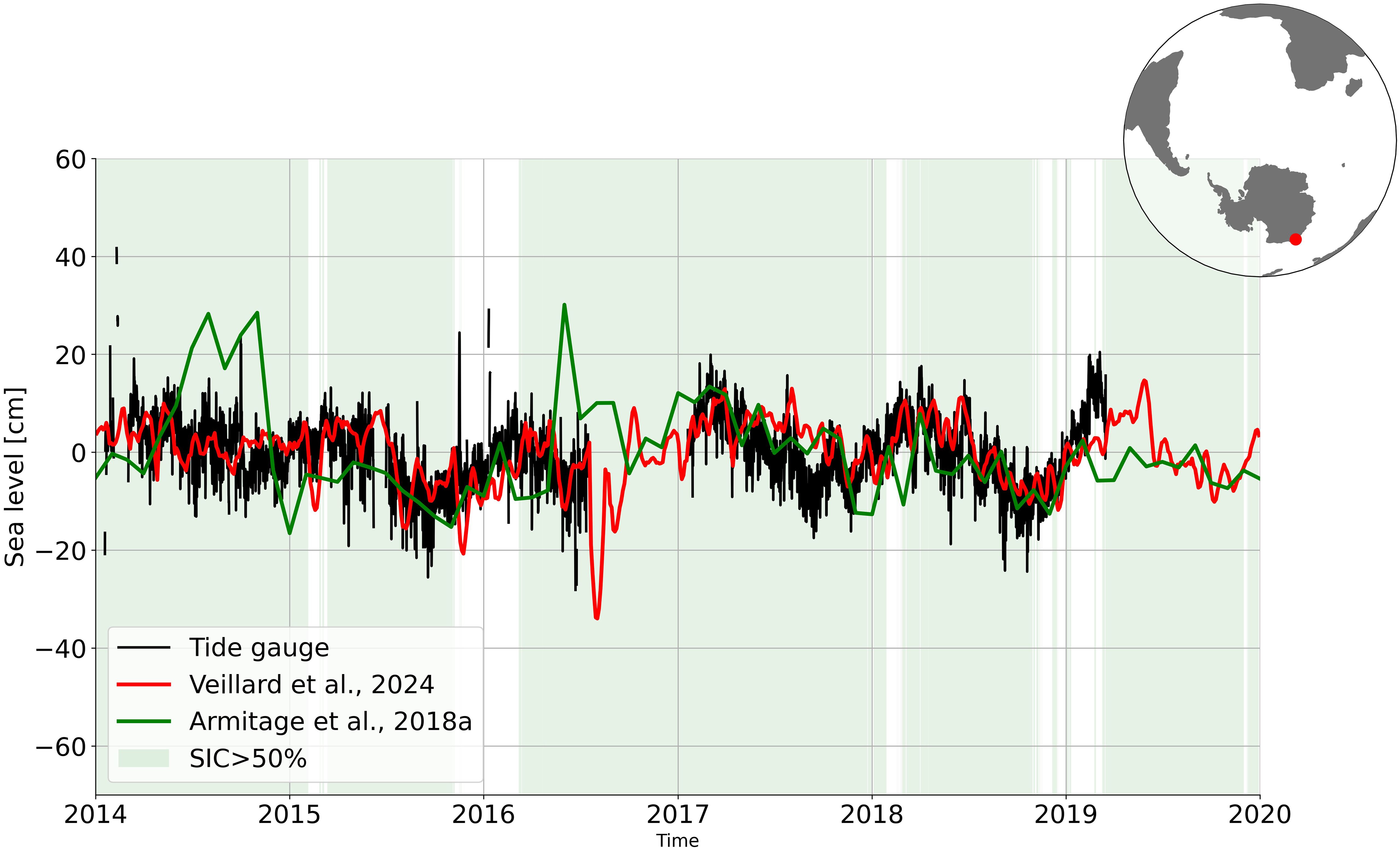
Figure 5. Southern Ocean SLA maps from current paper (red) and Armitage et al. (2018a) (green) vs. Dumont D’Urville tide gauge (black). Green shades denote periods when the sea ice concentration is over 50%. The altimetry nearest grid node from the TG is selected.
Our regional polar sea level products are also compared with BPR data for which we expect a correlation at timescales up to around 100 days (Vinogradova et al., 2007). Our regional Arctic product SLA is compared with the north pole BPR in Figure 6 in a region covered with ice throughout the year. The correlation is moderate at monthly timescales with a correlation of 0.56 for timescales below 60 days. Other comparisons are made with BPR in seasonally ice-covered regions (against BPR-A in the Beaufort Sea in Supplementary Figure 7 with a correlation of 0.55 for periods below 60 days and against BPR ANT-17.1 in the Southern Ocean in Supplementary Figure 8 with a correlation of 0.29 for period below 60 days).
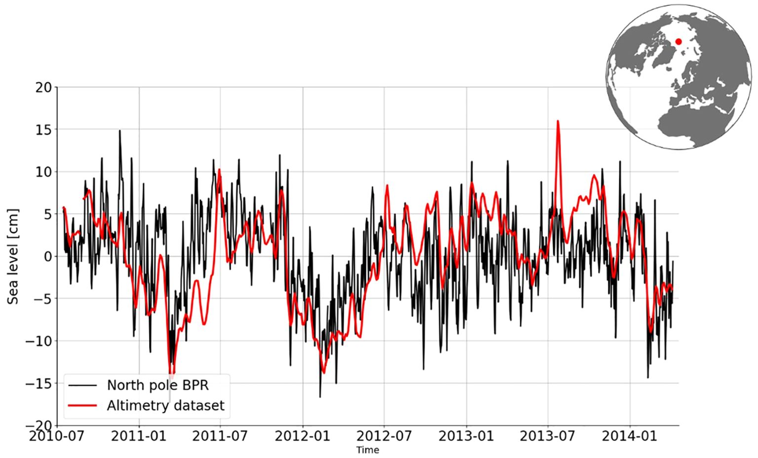
Figure 6. Arctic Ocean SLA maps (red) vs. north pole BPR (black). The altimetry nearest grid node from the BPR is selected.
4.4 Comparison with Arctic atmospheric circulation
Arctic sea level variability has been related to the atmospheric circulations through the Arctic Oscillation index (Morison et al., 2012; Armitage et al., 2018b). Positive (negative) Arctic Oscillation phases are associated with cyclonic (anticyclonic) wind circulation over the Arctic Ocean, causing sea levels to rise (drop) in the shallow coastal region via Ekman transport, and conversely the sea level to drop (rise) in the deep ocean (Armitage et al., 2018b). Figure 7A presents the map of the correlation coefficient (Pearson’s) between our regional Arctic L4 sea level product and the Arctic Oscillation index showing an opposite correlation between the shallow coastal region and the deep region of the Arctic Ocean, as observed in Armitage et al. (2018b). The limit between the two regions clearly follows the 300-m bathymetry contour (black dotted line) except along Greenland and Canadian Arctic Archipelago coasts and in the north part of the Barents Sea. The current dataset, with improved resolution compared with Armitage et al. (2018b), enables to see small features of correlation following the bathymetry contour in the seasonally ice-covered Barents Sea and North Sea. Contrary to the central Arctic, in the Gulf of Alaska, the coast is north of the sea and the correlation patterns are inverted with higher correlation in the deeper ocean. The wind-driven sea level evolution in the deeper Arctic Ocean region has been found to experience a near-uniform fluctuation (Fukumori et al., 2015). As shown in Figure 7B, time series of the inverse of the Arctic Oscillation is plotted against our altimetry sea level in the deeper basin Arctic region (defined as the region correlated negatively with the Arctic Oscillation and latitude over 70°N). A moderate correlation is found between the two time series at short time scales. For a period below 60 days, the correlation is 0.45; for longer periods, the sea level is dominated by other processes and correlation decreases. In short, at a monthly timescale, the Arctic altimetry sea level maps are shown to respond essentially to the wind-driven Arctic Oscillation during ice-free and ice-covered periods.
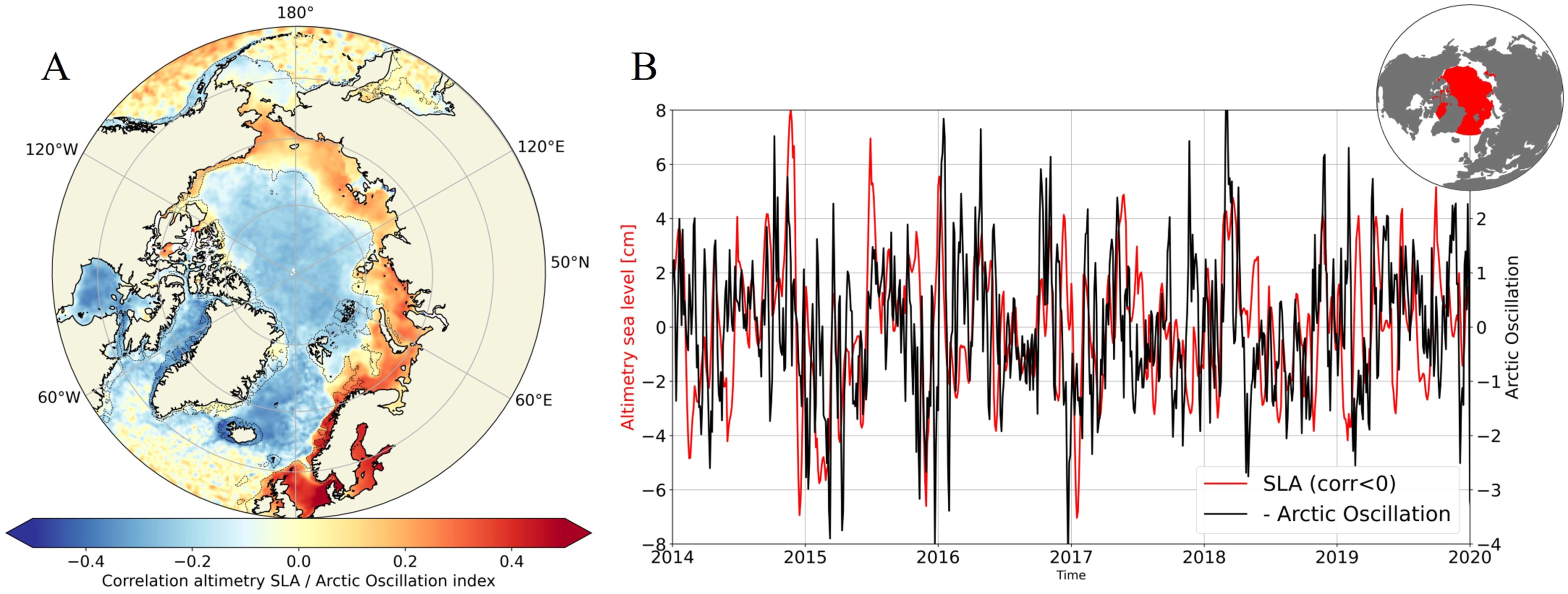
Figure 7. Correlation coefficient (Pearson’s) between altimetry SLA and Arctic Oscillation once seasonal and long-term signals have been removed to both data (A). The black dotted line denotes the 300-m iso-bathymetry. (B) Time series of altimetry SLA (for regions with a negative correlation in (A) and latitude over 70°N) and time series of the inverse of the Arctic Oscillation index. Long-term and seasonal cycles have been removed from both series.
In the coastal Laptev Sea region, local wind is better correlated with sea level than the regional Arctic Oscillation index. The zonal component of the local wind induces most of the cross-shelf Ekman transport in the Laptev Sea since the Laptev coasts are oriented longitudinally. Here, we use this approximation to compare our regional Arctic altimetry L4 sea level product to zonal modeled wind in the Laptev Sea in Figure 8. The two signals show coherent variations at a monthly timescale with a correlation of 0.64 for timescales below 60 days. The correlation between the two signals mainly remains when the region is ice-covered (periods with green shades).
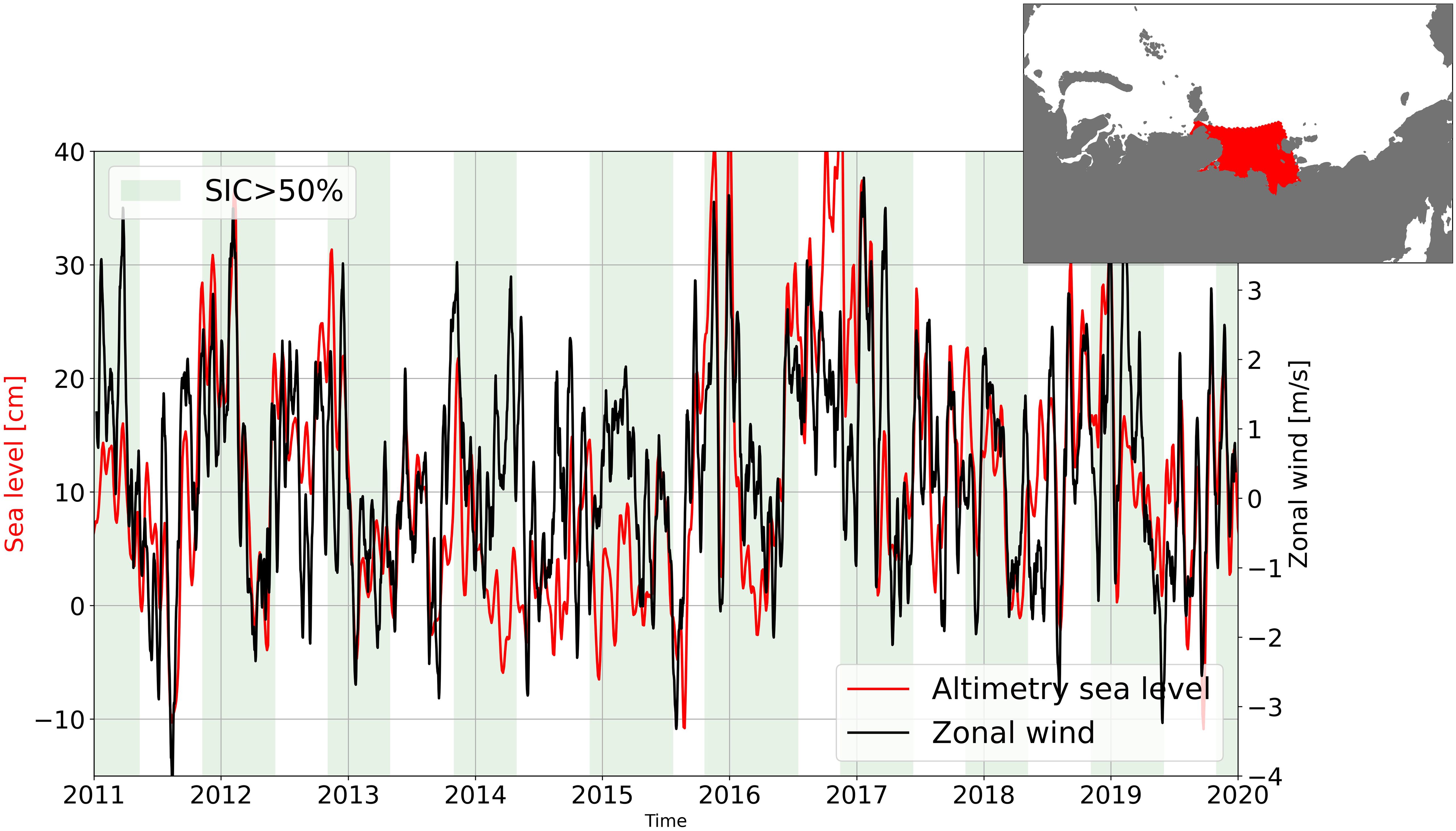
Figure 8. Altimetry SLA (red) and modeled zonal wind (black) in the Laptev Sea region [100°E, 140°E, 65°N, 78°N] shown on the upper right. Green shades denote periods when the sea ice concentration is over 50%.
4.5 At long-term
Long-term sea level evolutions of the products are analyzed here. In Figure 9A, the map of our regional Arctic sea level trends over the period 2011–2021 is plotted. Our Arctic Ocean trends are like the one observed with the DUACS product on the open ocean (not shown). Most of the seasonally ice-covered Arctic basin experiences a positive trend around the global open ocean one around 3 mm/year. It is quite different from the map of sea level trend estimates of Ludwigsen et al. (2022) using Rose et al.’s (2019) dataset over the period 1995–2015. Over this older period, Ludwigsen et al. (2022) found negative trends over Laptev Sea and around Greenland.
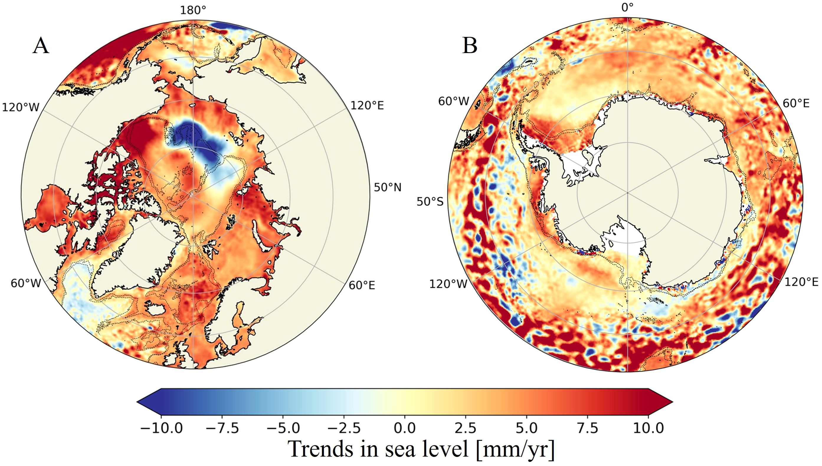
Figure 9. Map of altimetry sea level trends from 01/01/2011 to 01/01/2022 from for the Arctic Ocean (A) and from 01/01/2013 to 01/01/2022 for the Southern Ocean product (B).
In the Beaufort Sea, the Beaufort gyre experiences interannual variability with evolution of its freshwater storage (Timmermans and Toole, 2023). In that region, our Arctic L4 sea level trends are increased up to 15 mm/year (from the Canadian coast to 75°N in latitude and from 130°W to 150°W in longitude). It roughly corresponds to the region where freshwater has been increasing over the study period in Timmermans and Toole (2023). However, in Timmermans and Toole (2023), the region goes a little more eastward up to 160°W and starts farthest north not directly at the coast. In-situ T/S profile measurements at the BGEP A location in the Beaufort gyre are used to compare steric with altimetry sea level. In Figure 10, the in-situ steric height and the colocalized long-term altimetry SLA (1-year rolling mean) are plotted. The interannual evolutions are well correlated between the two time series with a sea level rise till mid-2019, corresponding to freshwater accumulation over the last years (Timmermans and Toole, 2023). A decrease is seen from mid-2019 that may be due to the evolution in shape of the Beaufort gyre and to freshwater decrease. In Timmermans and Toole (2023), the total freshwater content in the Beaufort gyre have decreased since approximately 2019. Using data up to 2019, Lin et al. (2023) also noted that the Beaufort Gyre has transitioned to a quasi-stable state in which the increase in sea surface height of the gyre has slowed.
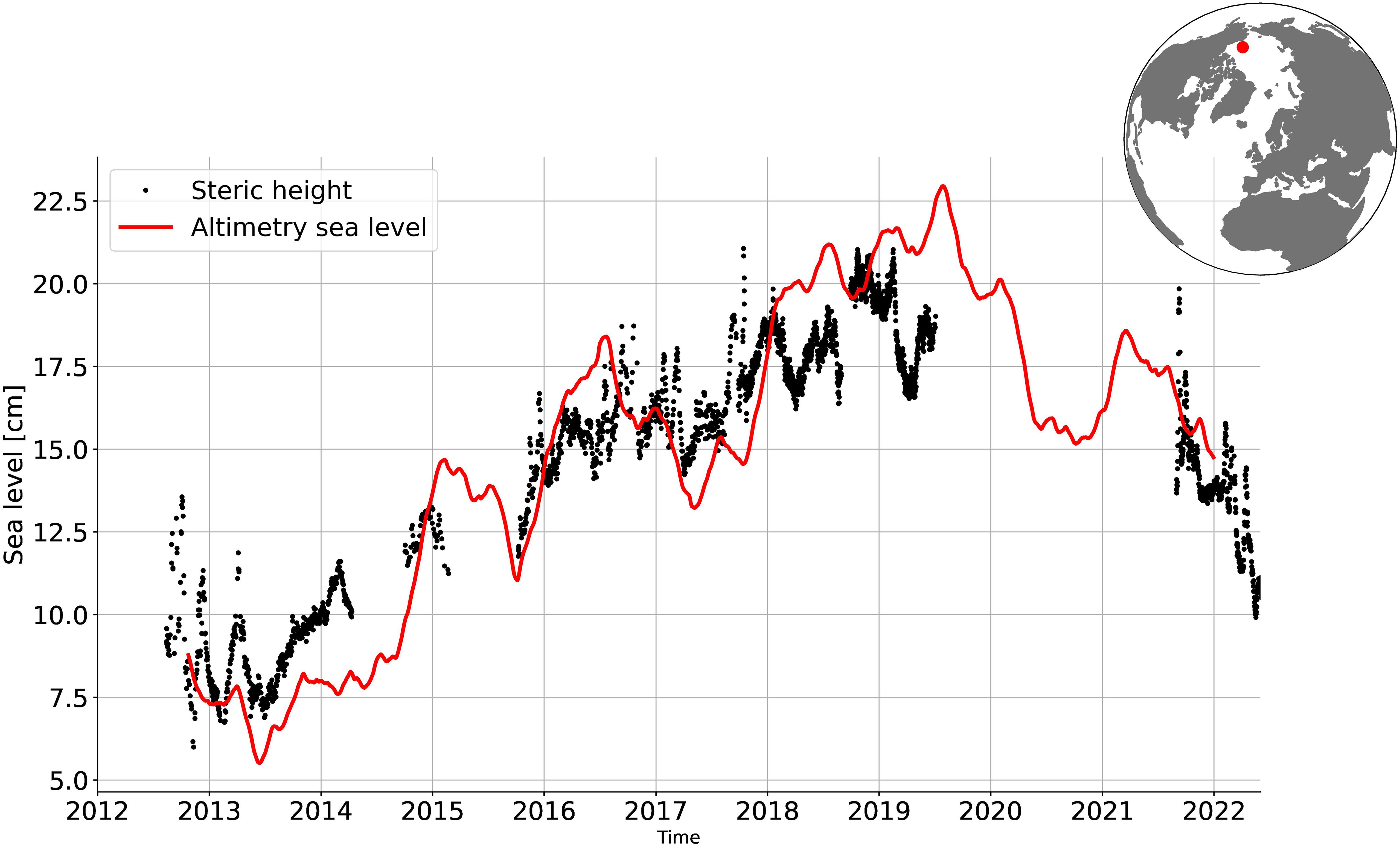
Figure 10. Steric height anomaly from in-situ profilers (black) and altimetry SLA (1-year rolling mean, red line) at the Beaufort Gyre Exploration Project A location. The altimetry nearest grid node from the profilers is selected.
The most striking feature on the map of our regional Arctic Sea level trends (Figure 9A) is a region with a negative trend up to −10 mm/year in the East Siberian Sea slope region, north of the Siberian Sea at the limit between the shallow and the deep Arctic region. This region of negative trends is slightly visible on the open ocean only DUACS DT21 sea level trends map (not shown). In that region, the sea level experiences a sharp decrease in 2016–2017, as observed in Bertosio et al. (2022), using Mercator Ocean Global Operational System GLORYS12V1. Bertosio et al. (2022) noted that the East Siberian slope region experienced a decrease of freshwater content after 2012 coherent with a shoaling of the warm and salty Atlantic waters. Hall et al. (2023) also found that this region experienced freshwater diminution using the Ocean Reanalysis System 5 model with a 2-m lower freshwater content over the period 2008–2018 compared with 1997–2007.
In Supplementary Figure 9, our regional Arctic sea level product and PSMSL tide gauges trends are plotted over the Arctic Ocean. Overall, similar trends are observed even if some tide gauges trends depart locally. It should be noted that some TG sea level time series are not available for the whole altimetry period and may be in coastal regions with different sea level variability.
The map of our Southern Ocean sea level trends over the period 2013–2021 is plotted in Figure 9B. Compared with DUACS sea level trends using only the open ocean regions with negative trends in the Ross Sea (not shown), the Southern Ocean dataset including the ice-covered region shows positive trends around 3 mm/year in the Ross Sea. In the south-west of the Weddell Sea, increased trends are observed up to 10 mm/year near the Antarctic Peninsula in the west. Increased trends are also observed on the coastal region of the Amundsen Sea.
5 Discussion
Multi-mission sea level maps and along-tracks are produced from altimetry including the ice-covered regions over a 10-year period. In the Arctic, our products start with Cryosat-2 providing first coverage up to 88°N. The use of several missions and the mapping enables to map smaller scales than other existing mono-mission products. Validations are made against in-situ data, showing that our regional polar products sample monthly variability during ice-covered regions. At interannual timescales, the Arctic sea level evolutions are mostly related to atmospheric circulations. Our Arctic sea level trends over a 10-year period are produced, showing a striking sea level decrease in the East Siberian slope region associated with freshwater decrease.
The product presented in this paper remains imperfect. Different limitations related to processing imperfections have been identified. Here, we present some of the limits of our products.
Melt ponds are formed in summer on the top of the sea ice in the Arctic Ocean (Webster et al., 2022). They are specular water surfaces on top of sea ice that are observed similarly to sea-ice leads that are water surfaces surrounded by sea ice by satellite altimeters. It is not wanted to observe melt pond heights for sea level products, but as currently we have no solution to differentiate a measurement over a melt pond from one over ice–ice lead, they may be present in our product. Here, we assess the observability of melt ponds in the products by comparing our regional Arctic sea level L4 product to melt pond fractions in summer 2016 (Figures 11A, B). SLA is abnormally high and noisy where melt pond fractions are high, indicating that melt ponds are certainly observed in the polar products during summer periods. Figure 11C presents the histogram of along-track SLA observations where melt ponds are present north of Greenland in June 2016. It shows two population of SLA, one corresponding to sea-ice lead observations and another one probably corresponding to melt pond height (i.e., sea ice height). The two populations are superimposed, so it is difficult to differentiate melt ponds from sea-ice lead observations and other strategies should be used. The Southern Ocean should be less subject to melt pond formations, and no melt pond observations were clearly identified.
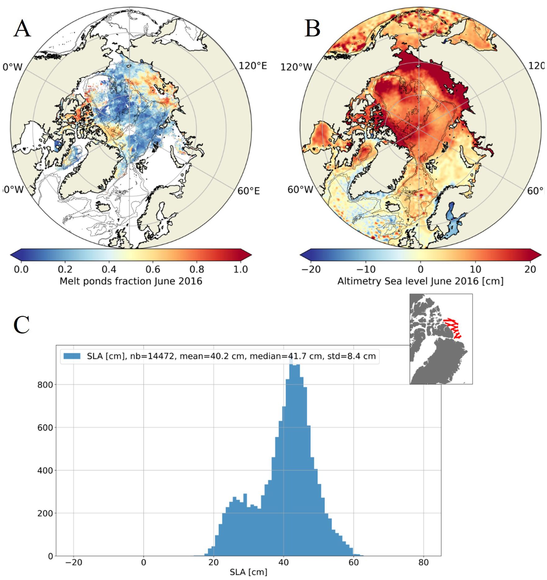
Figure 11. Melt pond fractions (A), and corresponding sea level from altimetry (B) for June 2016 showing abnormally high SLA where melt pond fractions are the highest. (C) Histogram of CryoSat-2 SLA showing both sea-ice leads sea level and melt pond heights for 20/06/2016 to 25/06/2016 north of Greenland (tracks on the upper right).
Our regional polar sea level products are assumed to be continuous between open ocean and sea-ice lead observations using the continuous Adaptive retracking between the two surfaces (Poisson et al., 2018; Tourain et al., 2021). However, discontinuities may arise from different factors. Firstly, the retracker operates on sea-ice leads and open ocean waveforms using the same sampling, and for very peaky sea-ice lead echoes, few points are used to estimate the range and instrumental studies are needed to quantify this impact on the estimated range. Moreover, other factors may bring discontinuities such as wrong identification of surfaces (open ocean, sea-ice leads, melt ponds) and absence of continuity in the satellite corrections. Satellite corrections are found to be continuous at the limit between the two surfaces with differences below 1 cm for most of the corrections except for the SSB correction as expected, since it is not applied to sea-ice lead SLA. SSB correction induces open ocean SLA to be ~4 cm higher than sea-ice lead SLA. SSB is not applied to sea-ice lead SLA under the assumption that wind and waves are negligible. That may be questioned especially for the Southern Ocean where waves have higher amplitudes and were observed up to 200 km within the Antarctic marginal ice zone (Brouwer et al., 2022). The Dynamical Atmospheric correction may also be involved in a bias since the barotropic model used for this correction does not consider sea-ice cap feedback (Carrere et al., 2016) and may not be valid for the sea-ice leads. Finally, geophysical processes such as localized wind-driven process (Campbell, 1965) or brine rejection may bring discontinuity between open ocean and sea-ice lead sea level. The bias between sea-ice lead SLA and open ocean SLA is estimated at the limit between the two surfaces using 75-km/10-day boxes containing both open ocean and sea-ice lead observations. The bias is found to be ~5 cm for the Arctic Ocean (considering the summer period that may be affected by melt ponds observations) and ~3 cm for the Southern Ocean (see distribution in Supplementary Figure 10). Spatial patterns of the bias (Supplementary Figure 11) and its seasonal evolution with higher bias in summer (not shown) need to be analyzed. However, these biases are associated with great uncertainty due to the few data available and the increased uncertainty in this region.
A new innovative mapping strategy such as the multiscale and multivariate mapping approach explored in Ballarotta et al. (2023) or the Bayesian approach (Gregory et al., 2021; Landy et al., 2021) may be used for next versions of our regional polar products. In the future, the aim is to produce sea-ice lead data in operational mode that can be combined with open ocean observations. However, differences are present between the polar datasets that are calibrated on SARAL/AltiKa and the global ocean DUACS datasets calibrated on the Jasons satellites that are limited to an orbit of 66°. The time series of differences between our regional polar sea level maps and DUACS DT21 open ocean maps are plotted in Supplementary Figures 12, 13, showing an annual seasonal signal (9 mm for the Arctic Ocean and 4 mm for the Southern Ocean) and a long-term trend (−0.09 mm/year for the Arctic Ocean and −0.01 mm/year for the Southern Ocean). For finer calibration, orbit error (Le Traon and Ogor, 1998) may be used in future polar products to calibrate polar data with DUACS open ocean data for homogeneity and consistency at long-term.
The product provides data since 2011 in the Arctic region starting with first Cryosat-2 data enabling to map data up to 88°N. The product can be extended backward thanks to former satellites such as ENVISAT; however, coverage will only map up to 81.5°N that is sufficient for Southern Ocean but provides a gap for the Arctic Ocean.
New satellites have been launched to complement classical radar missions. ICESat-2 laser mission provides valuable data in the sea-ice leads to complement the radar missions. The SWOT (Surface Water Ocean Topography) mission also challenges the current observations in the ice-covered regions with 60-km-wide swath observations up to 77.6° and should provide new understandings of the polar region. New missions are also to be launched as CRISTAL (Copernicus Polar Ice and Snow Topography Altimeter) to continue to monitor the polar region. These missions should also bring improvements to the corrections used by altimetry (MSS, tide, DAC) to better understand these regions in a changing climate.
Data availability statement
The datasets presented in this study can be found in online repositories. The names of the repository/repositories and accession number(s) can be found here: https://www.aviso.altimetry.fr/en/data/products/sea-surface-height-products/regional/arctic-ocean-sea-level-heights.html; https://www.aviso.altimetry.fr/en/data/products/sea-surface-height-products/regional/antarctic-sea-level-heights.html.
Author contributions
PV: Conceptualization, Data Curation, Formal analysis, Methodology, Validation, Writing – original draft, Writing – review & editing. PP: Conceptualization, Methodology. M-IP: Writing – review & editing, Supervision. J-AD: Data Curation, Methodology, Writing – review & editing. FP: Data Curation, Methodology, Writing – review & editing. GD: Writing – review & editing, Supervision. YF: Writing – review & editing, Supervision.
Funding
The author(s) declare financial support was received for the research, authorship, and/or publication of this article. This work was financially and technically supported by the Centre National d’Etudes Spatiales (CNES) in the frame of the DUACS R&D project (contract number 20221).
Acknowledgments
The authors thanks all the people that contributed to this work, including Matthis Auger, Cosme Mosneron Dupin, and Gregory Smith, that tested the demonstration altimeter product and through their feedback contributed to its development.
Conflict of interest
The authors declare that the research was conducted in the absence of any commercial or financial relationships that could be construed as a potential conflict of interest.
Publisher’s note
All claims expressed in this article are solely those of the authors and do not necessarily represent those of their affiliated organizations, or those of the publisher, the editors and the reviewers. Any product that may be evaluated in this article, or claim that may be made by its manufacturer, is not guaranteed or endorsed by the publisher.
Supplementary material
The Supplementary Material for this article can be found online at: https://www.frontiersin.org/articles/10.3389/fmars.2024.1419132/full#supplementary-material
References
Androsov A., Boebel O., Schröter J., Danilov S., Macrander A., Ivanciu I. (2020). Ocean bottom pressure variability: can it be reliably modeled? J. Geophysical Res.: Oceans 125. doi: 10.1029/2019jc015469
Armitage T. W. K., Bacon S., Kwok R. (2018b). Arctic sea level and surface circulation response to the arctic oscillation. Geophysical Res. Lett. 45, 6576–6584. doi: 10.1029/2018gl078386
Armitage T. W. K., Bacon S., Ridout A. L., Thomas S. F., Aksenov Y., Wingham D. J. (2016). Arctic sea surface height variability and change from satellite radar altimetry and GRACE 2003–2014. J. Geophysical Res.: Oceans 121, 4303–4322. doi: 10.1002/2015jc011579
Armitage T. W. K., Kwok R., Thompson A. F., Cunningham G. (2018a). Dynamic topography and sea level anomalies of the southern ocean: variability and teleconnections. J. Geophysical Res.: Oceans 123, 613–630. doi: 10.1002/2017jc013534
Auger M., Prandi P., Sallée J.-B. (2022). Southern ocean sea level anomaly in the sea ice-covered sector from multimission satellite observations. Sci. Data 9. doi: 10.1038/s41597-022-01166-z
Bagnardi M., Kurtz N. T., Petty A. A., Kwok R. (2021). Sea surface height anomalies of the Arctic Ocean from ICESat-2: A first examination and comparisons with CryoSat-2. Geophysical Res. Lett. 48. doi: 10.1029/2021gl093155
Ballarotta M., Ubelmann C., Veillard P., Prandi P., Etienne H., Mulet S., et al. (2023). Improved global sea surface height and current maps from remote sensing and in situ observations. In Earth Sys. Sci. Data 15, 295–315. doi: 10.5194/essd-15-295-2023
Bertosio C., Provost C., Athanase M., Sennéchael N., Garric G., Lellouche J., et al. (2022). Changes in freshwater distribution and pathways in the Arctic Ocean since 2007 in the Mercator Ocean global operational system. J. Geophysical Res.: Oceans 127. doi: 10.1029/2021jc017701
Bretherton F. P., Davis R. E., Fandry C. B. (1976). A technique for objective analysis and design of oceanographic experiments applied to MODE-73. Deep Sea Res. Oceanographic Abstracts 23, 559–582. doi: 10.1016/0011-7471(76)90001-2
Brodzik M. J., Billingsley B., Haran T., Raup B., Savoie M. H. (2012). EASE-grid 2.0: incremental but significant improvements for earth-gridded data sets. ISPRS Int. J. Geo-Information 1, 32–45. doi: 10.3390/ijgi1010032
Brouwer J., Fraser A. D., Murphy D. J., Wongpan P., Alberello A., Kohout A., et al. (2022). Altimetric observation of wave attenuation through the Antarctic marginal ice zone using ICESat-2. Cryosphere 16, 2325–2353. doi: 10.5194/tc-16-2325-2022
Caldwell P. C., Merrifield M. A., Thompson P. R. (2001). Sea level measured by tide gauges from global oceans as part of the Joint Archive for Sea Level (JASL) since 1846 (NOAA National Centers for Environmental Information). doi: 10.7289/V5V40S7W
Campbell W. J. (1965). The wind-driven circulation of ice and water in a polar ocean. J. Geophysical Res. 70, 3279–3301. doi: 10.1029/jz070i014p03279
Carrère L., Lyard F. (2003). Modeling the barotropic response of the global ocean to atmospheric wind and pressure forcing - comparisons with observations. Geophysical Res. Lett. 30. doi: 10.1029/2002gl016473
Carrere L., Faugère Y., Ablain M. (2016). Major improvement of altimetry sea level estimations using pressure-derived corrections based on ERA-Interim atmospheric reanalysis. Ocean Sci. 12, 825–842. doi: 10.5194/os-12-825-2016
Carrere L., Lyard F., Cancet M., Allain D., Dabat M.-L., Fouchet E., et al. (2022). A new barotropic tide model for global ocean: FES2022 (CNES) Venezia (Italy). doi: 10.24400/527896/A03-2022.3287.
Cartwright D. E., Edden A. C. (1973). Corrected tables of tidal harmonics. Geophysical J. Int. 33, 253–264. doi: 10.1111/j.1365-246x.1973.tb03420.x
Danielson S. L., Hennon T. D., Hedstrom K. S., Pnyushkov A. V., Polyakov I. V., Carmack E., et al. (2020). Oceanic routing of wind-sourced energy along the Arctic Continental shelves. Front. Mar. Sci. 7. doi: 10.3389/fmars.2020.00509
Desai S., Wahr J., Beckley B. (2015). Revisiting the pole tide for and from satellite altimetry. J. Geodesy 12, 1233–1243. doi: 10.1007/s00190-015-0848-7
Doglioni F., Ricker R., Rabe B., Barth A., Troupin C., Kanzow T. (2023). Sea surface height anomaly and geostrophic current velocity from altimetry measurements over the Arctic Ocean, (2011–2020). Earth Sys. Sci. Data 15, 225–263. doi: 10.5194/essd-15-225-2023
Dotto T. S., Naveira Garabato A., Bacon S., Tsamados M., Holland P. R., Hooley J., et al. (2018). Variability of the Ross Gyre, Southern Ocean: drivers and responses revealed by satellite altimetry. Geophysical Res. Lett. 45, 6195–6204. doi: 10.1029/2018gl078607
Ducet N., Le Traon P. Y., Reverdin G. (2000). Global high-resolution mapping of ocean circulation from TOPEX/Poseidon and ERS-1 and -2. J. Geophysical Res.: Oceans 105, 19477–19498. doi: 10.1029/2000jc900063
Faugère Y., Taburet G., Ballarotta M., Pujol I., Legeais J. F., Maillard G., et al. (2022). DUACS DT2021: 28 years of reprocessed sea level altimetry products (Copernicus GmbH) Venezia (Italy). doi: 10.5194/egusphere-egu22-7479
Fukumori I., Wang O., Llovel W., Fenty I., Forget G. (2015). A near-uniform fluctuation of ocean bottom pressure and sea level across the deep ocean basins of the Arctic Ocean and the Nordic Seas. Prog. Oceanogr. 134, 152–172. doi: 10.1016/j.pocean.2015.01.013
Gregory W., Lawrence I. R., Tsamados M. (2021). A Bayesian approach towards daily pan-Arctic sea ice freeboard estimates from combined CryoSat-2 and Sentinel-3 satellite observations. Cryosphere 15, 2857–2871. doi: 10.5194/tc-15-2857-2021
Hall S. B., Subrahmanyam B., Steele M. (2023). The role of the Russian shelf in seasonal and interannual variability of Arctic sea surface salinity and freshwater content. J. Geophysical Res.: Oceans 128. doi: 10.1029/2022jc019247
Holgate S. J., Matthews A., Woodworth P. L., Rickards L. J., Tamisiea M. E., Bradshaw E., et al. (2013). New data systems and products at the permanent service for mean sea level. J. Coast. Res. 29, 493–504. doi: 10.2112/jcoastres-d-12-00175.1
Holland D. M., Nicholls K. W., Basinski A. (2020). The Southern Ocean and its interaction with the Antarctic Ice Sheet. Science 367, 1326–1330. doi: 10.1126/science.aaz5491
Iijima B. A., Harris I. L., Ho C. M., Lindqwister U. J., Mannucci A. J., Pi X., et al. (1999). Automated daily process for global ionospheric total electron content maps and satellite ocean altimeter ionospheric calibration based on Global Positioning System data. J. Atmospheric Solar-Terrestrial Phys. 61, 1205–1218. doi: 10.1016/s1364-6826(99)00067-x
Jettou G., Rousseau M., Piras F., Simeon M., Tran N. (2023). SARAL’s full mission reprocessing: improvement with the GDR-F standard. Remote Sens. 15, 2604. doi: 10.3390/rs15102604
Jones E. P., Anderson L. G., Swift J. H. (1998). Distribution of Atlantic and Pacific waters in the upper Arctic Ocean: Implications for circulation. Geophysical Res. Lett. 25, 765–768. doi: 10.1029/98gl00464
Jousset S. (2023). Mean Dynamic Topography MDT CNES_CLS 2022 (Version 2022) (CNES). doi: 10.24400/527896/A01-2023.003
Kwok R., Petty A. A., Cunningham G., Markus T., Hancock D., Ivanoff A., et al. (2021). ATLAS/ICESat-2 L3A Sea Ice Height, Version 5 (Boulder, Colorado USA: NASA National Snow and Ice Data Center Distributed Active Archive Center). doi: 10.5067/ATLAS/ATL07.005
Laloue A., Schaeffer P., Pujol M.-I., Veillard P., Andersen O. B., Sandwell D. T., et al. (2024). Merging recent Mean Sea Surface into a 2023 Hybrid model (from Scripps, DTU, CLS and CNES) (Authorea, Inc). doi: 10.22541/au.171987154.42384510/v1
Landy J. C., Bouffard J., Wilson C., Rynders S., Aksenov Y., Tsamados M. (2021). Improved Arctic Sea ice freeboard retrieval from satellite altimetry using optimized sea surface decorrelation scales. J. Geophysical Res.: Oceans 126. doi: 10.1029/2021jc017466
Lee S., Stroeve J. (2021). Arctic Melt Pond Fraction and Binary Classification 2000-2020 (1.0) (UK Polar Data Centre, Natural Environment Research Council, UK Research & Innovation). doi: 10.5285/B91EA195-FD3D-4171-BAE4-198C46575C16
Le Traon P. Y., Nadal F., Ducet N. (1998). An improved mapping method of multisatellite altimeter data. J. Atmospheric Oceanic Technol. 15, 522–534). doi: 10.1175/1520-0426(1998)015<0522:aimmom>2.0.co;2
Le Traon P.-Y., Ogor F. (1998). ERS-1/2 orbit improvement using TOPEX/POSEIDON: The 2 cm challenge. J. Geophysical Res.: Oceans 103, 8045–8057. doi: 10.1029/97jc01917
Lin P., Pickart R. S., Heorton H., Tsamados M., Itoh M., Kikuchi T. (2023). Recent state transition of the Arctic Ocean’s Beaufort Gyre. Nat. Geosci. 16, 485–491. doi: 10.1038/s41561-023-01184-5
Ludwigsen C. B., Andersen O. B., Rose S. K. (2022). Components of 21 years, (1995–2015) of absolute sea level trends in the Arctic. Ocean Sci. 18, 109–127. doi: 10.5194/os-18-109-2022
Morison J., Kwok R., Peralta-Ferriz C., Alkire M., Rigor I., Andersen R., et al. (2012). Changing Arctic Ocean freshwater pathways. Nature 481, 66–70. doi: 10.1038/nature10705
Naveira Garabato A. C., Dotto T. S., Hooley J., Bacon S., Tsamados M., Ridout A., et al. (2019). Phased response of the subpolar southern ocean to changes in circumpolar winds. Geophysical Res. Lett. 46, 6024–6033. doi: 10.1029/2019gl082850
Peacock N. R., Laxon S. W. (2004). Sea surface height determination in the Arctic Ocean from ERS altimetry. J. Geophysical Res.: Oceans 109. doi: 10.1029/2001jc001026
Peltier W. R. (2004). GLOBAL GLACIAL ISOSTASY AND THE SURFACE OF THE ICE-AGE EARTH: the ICE-5G (VM2) model and GRACE. Annu. Rev. Earth Planetary Sci. 32, 111–149. doi: 10.1146/annurev.earth.32.082503.144359
Permanent Service for Mean Sea Level (PSMSL) (2024). Tide Gauge Data. Available online at: http://www.psmsl.org/data/obtaining/. [August 1, 2024]
Poisson J.-C., Quartly G. D., Kurekin A. A., Thibaut P., Hoang D., Nencioli F. (2018). Development of an ENVISAT altimetry processor providing sea level continuity between open ocean and Arctic leads. IEEE Trans. Geosci. Remote Sens. 56, 5299–5319. doi: 10.1109/tgrs.2018.2813061
Prandi P., Poisson J.-C., Faugère Y., Guillot A., Dibarboure G. (2021). Arctic sea surface height maps from multi-altimeter combination. Earth Sys. Sci. Data 13, 5469–5482. doi: 10.5194/essd-13-5469-2021
Quartly G. D., Rinne E., Passaro M., Andersen O. B., Dinardo S., Fleury S., et al. (2019). Retrieving sea level and freeboard in the arctic: A review of current radar altimetry methodologies and future perspectives. Remote Sens. 11, 881. doi: 10.3390/rs11070881
Rantanen M., Karpechko A., Lipponen A., Nordling K., Hyvärinen O., Ruosteenoja K., et al. (2022). The Arctic has warmed nearly four times faster than the globe since 1979. Commun. Earth Environ. 3. doi: 10.1038/s43247-022-00498-3
Rintoul S. R. (2018). The global influence of localized dynamics in the Southern Ocean. Nature 558, 209–218. doi: 10.1038/s41586-018-0182-3
Rose S. K., Andersen O. B., Passaro M., Ludwigsen C. A., Schwatke C. (2019). Arctic Ocean sea level record from the complete radar altimetry era: 1991–2018. Remote Sens. 11, 1672. doi: 10.3390/rs11141672
Schaeffer P., Pujol M.-I., Veillard P., Faugere Y., Dagneaux Q., Dibarboure G., et al. (2023). The CNES CLS 2022 mean sea surface: short wavelength improvements from CryoSat-2 and SARAL/altiKa high-sampled altimeter data. Remote Sens. 15, 2910. doi: 10.3390/rs15112910
Smith G. C., Allard R., Babin M., Bertino L., Chevallier M., Corlett G., et al. (2019). Polar ocean observations: A critical gap in the observing system and its effect on environmental predictions from hours to a season. Front. Mar. Sci. 6. doi: 10.3389/fmars.2019.00429
Taburet G., Sanchez-Roman A., Ballarotta M., Pujol M.-I., Legeais J.-F., Fournier F., et al. (2019). DUACS DT2018: 25 years of reprocessed sea level altimetry products. Ocean Sci. 15, 1207–1224. doi: 10.5194/os-15-1207-2019
Timmermans M., Marshall J. (2020). Understanding Arctic Ocean circulation: A review of ocean dynamics in a changing climate. J. Geophysical Res.: Oceans 125. doi: 10.1029/2018jc014378
Timmermans M.-L., Toole J. M. (2023). The Arctic Ocean’s Beaufort gyre. Annu. Rev. Mar. Sci. 15, 223–248. doi: 10.1146/annurev-marine-032122-012034
Tourain C., Piras F., Ollivier A., Hauser D., Poisson J. C., Boy F., et al. (2021). Benefits of the adaptive algorithm for retracking altimeter nadir echoes: results from simulations and CFOSAT/SWIM observations. IEEE Trans. Geosci. Remote Sens. 59, 9927–9940. doi: 10.1109/tgrs.2021.3064236
Tran N., Labroue S., Philipps S., Bronner E., Picot N. (2010). Overview and update of the sea state bias corrections for the Jason-2, Jason-1 and TOPEX missions. Mar. Geodesy 33, 348–362. doi: 10.1080/01490419.2010.487788
Vinogradova N. T., Ponte R. M., Stammer D. (2007). Relation between sea level and bottom pressure and the vertical dependence of oceanic variability. Geophysical Res. Lett. 34. doi: 10.1029/2006gl028588
Volkov D. L., Landerer F. W., Kirillov S. A. (2013). The genesis of sea level variability in the Barents Sea. In Continental Shelf Research (Vol. 66, pp. 92–104). Elsevier BV. doi: 10.1016/j.csr.2013.07.007
Keywords: satellite altimetry, Arctic Ocean, Southern Ocean, sea level change, Arctic Oscillation
Citation: Veillard P, Prandi P, Pujol M-I, Daguzé J-A, Piras F, Dibarboure G and Faugère Y (2024) Arctic and Southern Ocean polar sea level maps and along-tracks from multi-mission satellite altimetry from 2011 to 2021. Front. Mar. Sci. 11:1419132. doi: 10.3389/fmars.2024.1419132
Received: 17 April 2024; Accepted: 29 August 2024;
Published: 24 September 2024.
Edited by:
David Alberto Salas Salas De León, National Autonomous University of Mexico, MexicoReviewed by:
Raúl Aguirre-Gómez, National Autonomous University of Mexico, MexicoMichel Tsamados, University College London, United Kingdom
Stine Kildegaard Rose, DTU Space - National Space Institute, Denmark
Copyright © 2024 Veillard, Prandi, Pujol, Daguzé, Piras, Dibarboure and Faugère. This is an open-access article distributed under the terms of the Creative Commons Attribution License (CC BY). The use, distribution or reproduction in other forums is permitted, provided the original author(s) and the copyright owner(s) are credited and that the original publication in this journal is cited, in accordance with accepted academic practice. No use, distribution or reproduction is permitted which does not comply with these terms.
*Correspondence: Pierre Veillard, cHZlaWxsYXJkQGdyb3VwY2xzLmNvbQ==; Marie-Isabelle Pujol, bXB1am9sQGdyb3VwY2xzLmNvbQ==