The salinity anomalies due to nutrients and inorganic carbon in the Bohai Sea

As a new seawater standard, the International Thermodynamic Equation of Seawater-2010 (TEOS-10) has made it possible to accurately calculate salinity changes caused by small changes in the relative proportions of inorganic dissolved constituents in the open ocean and thus to accurately calculate the thermodynamic properties of seawater. However, offshore and semi-enclosed seas are subject to the dual influence of geo-biochemical processes and terrestrial inputs, and the spatial and temporal variations in the relative composition of their seawater are more complex, resulting in very few studies of salinity change due to changes in the relative composition in these regions, and the applicability of the TEOS-10 in these seas needs to be further evaluated. The Bohai Sea is a typical semi-enclosed sea that has accumulated a large amount of physical oceanography and marine chemistry measurements, making it an ideal area to study the effects of changes in the relative composition of seawater on salinity. Based on repeated measurements of Section B in the Bohai Sea from 1985 to 2020, complemented by quasi-synchronous large-scale measurements of the Bohai Sea from 2006 to 2007, this study found that $[{\text{HCO}}_3^{-}]$ and $[{\text{Ca}}^{2+}]$ ions anomalies dominate the relative composition anomalies of dissolved substances in this sea relative to the Standard Sea Water (SSW). These additional components could increase the absolute salinity $S_{\text{A}}$ by up to 0.1 g·kg^-1 and the practical salinity $S_{\text{P}}$ by 0~0.04 according to the TEOS-10 algorithm and the mathematical model Pa08. Based on the specific environmental characteristics of the Bohai Sea, the sources, spatial and temporal variations, and influencing factors of the relative compositional anomalies are analyzed, and the empirical formulas of the absolute salinity anomaly $\delta S_{\text{A}}$ and practical salinity anomaly $\delta S_{\text{P}}$ for the Bohai Sea are further fitted, with the uncertainty of 0.007~0.021 g·kg^-1 for $\delta S_{\text{A}}$ and 0.003~0.008 for $\delta S_{\text{P}}$. The above results can not only improve the accuracy of the thermodynamic properties of the Bohai Seawater, but also provide the compatibility level of the long-term salinity changes in the Bohai Sea and its adjacent waters.

1 Introduction

Salinity, as a fundamental parameter for quantifying the total mass fraction of dissolved substances in seawater, has been identified as the “Essential Climate Variable” for observing, modeling, and analyzing the effects of global warming on ecosystems and society by the Global Climate Observing System (GCOS, 2010). Maintaining consistency and compatibility in salinity data is crucial for ensuring precise and continuous long-term trends (Feistel et al., 2016; Pawlowicz et al., 2016). Consequently, conventional salinity research and monitoring demand an accuracy of 0.002g·kg^-1 for the mass fraction of dissolved substances in seawater (Seitz et al., 2011), while the uncertainty of CTD commonly utilized in current ocean surveys to obtain Practical Salinity data is closer of 0.0034 (PSS-78) relative to the Standard Sea Water (Le Menn, 2011; Uchida et al., 2020).

Direct measurements of seawater salinity pose challenges in operational observations due to the intricate nature of dissolved components. Current methods rely on the Marcet’s principle that major seawater constituents maintain the same constant concentration ratio as standard seawater (SSW). Salinity measurements involve measuring specific seawater properties, like chlorinity or conductivity, and fitting them to empirical equations. However, the existing observation indicate that small changes in the relative composition of seawater are likely to cause changes in seawater properties that exceed the measurement accuracy of instruments. TEOS-10 (IOC et al., 2010) provides a correction factor called ‘Absolute Salinity Anomalies’ (denoted by $\delta S_{\text{A}}$) which characterizes the impact of these relative composition changes on seawater density and is used to determine the Absolute Salinity ($S_{\text{A}}$). Studies reveal that $\delta S_{\text{A}}$ does vary among water bodies, ranging from 0 to 0.030 ± 0.01 g·kg^-1 in the open ocean (McDougall et al., 2012), to about 0.087 ± 0.028 g·kg^-1 in the Baltic Sea (Feistel et al., 2010), and spanning three orders of magnitude in estuaries, from 0.005 to 0.6 g·kg^-1 (Pawlowicz, 2015), and from -0.05 to 0.28 g·kg^-1 in the Chinese offshore (Ji et al., 2021), so site-specific $\delta S_{\text{A}}$ analyses and calculations are needed.

While the thermodynamic properties of seawater are contingent upon the absolute salinity $S_{\text{A}}$, contemporary salinity measurements and numerous salinity studies continue to use the practical salinity ($S_{\text{P}}$). Practical salinity, as the salinity parameter of the International Equation of State of Seawater 1980 (EOS-80) (UNESCO, 1981), has been used in oceanography society for more than thirty years. It is determined by the ratio of a seawater sample’s conductivity to that of SSW under specific conditions (i.e., 15°C temperature and 1 atmosphere pressure). Since nonconductive silicate and total alkalinity are the predominant compositional anomalies in the open ocean, they have less influence on practical salinity, resulting in fewer related studies. Pawlowicz (2008); (2010); (2011) quantified $\delta S_{\text{P}}$ due to relative dissolved compositional anomalies in the North Pacific Intermediate Waters (NPIW), revealing $\delta S_{\text{P}}$ to be approximately 0.0062. Consequently, contemporary studies examining long-term salinity changes tend to overlook anomalies in the relative composition of dissolved substances in seawater, instead focusing on practical salinity (Chen, 1992; Zweng et al., 2019).

However, the spatial and temporal variations in the relative composition of seawater in offshore and semi-enclosed seas are complicated influenced by geo-biochemical processes and terrestrial inputs. This complexity leads to a dearth of studies on practical salinity variations in these regions resulting from changes in relative composition. Pawlowicz (2015) addressed this by calculating $S_{\text{A}}$ solely based on the relative composition of climatological runoff, overlooking the substrate’s effect on seawater composition. Similarly, Ji et al. (2021) calculated absolute salinity $S_{\text{A}}$ in the Chinese offshore using measurements from 2006–2007 without exploring the absolute salinity changes in other time. And there are few studies on the practical salinity variation due to changes in the relative composition of seawater of these regions.

Since 1957, China has conducted continuous and comprehensive marine surveys and research in the semi-enclosed Bohai Sea, amassing a vast array of physical oceanographic and seawater chemistry data, including high-precision measurements with a spatial resolution of up to 10 kilometers. These data allow for the capture and analysis of complex geochemical processes across various spatial and temporal scales, facilitating the accurate calculation of salinity anomalies resulting from these processes.

Regrettably, existing studies on long-term salinity changes in the Bohai Sea, such as those by Lin et al. (2001); Ma et al. (2006); Xu (2007); Lv (2008), and Yu et al. (2009), do not account for these salinity anomalies. Particularly in winter, strong north winds transport water from the Bohai Sea to the Yellow Sea through the Bohai Strait, significantly impacting the salinity of the Yellow Sea. Therefore, gaining an accurate understanding of salinity changes in the Bohai Sea is not only crucial for studying the climate and ecological environment of the Bohai Sea itself but also provides valuable insights for studying adjacent seas.

The aforementioned scenario underscores the necessity of investigating salinity changes in the Bohai Sea resulting from alterations in the relative composition of local seawater. This study aims to address the following key inquiries: Firstly, what are the principal variations in the relative composition of Bohai Sea water compared to SSW? What are their spatial and temporal distribution characteristics, sources, and influencing factors? Secondly, what are the magnitude and distribution characteristics of resulting absolute salinity anomaly $\delta S_{\text{A}}$ and practical salinity anomaly $\delta S_{\text{P}}$ in the Bohai Sea? Thirdly, can empirical formulas be derived for $\delta S_{\text{A}}$ and $\delta S_{\text{P}}$ in the Bohai Sea? Lastly, can existing studies elucidate the compatibility magnitude of salinity in the Bohai Sea?

The structure of this paper is as follows: Section 2 provides the algorithms for $\delta S_{\text{A}}$ and $\delta S_{\text{P}}$, along with a presentation of the data used in the study. Section 3 elaborates on the relative compositional anomalies, the magnitudes of $\delta S_{\text{A}}$ and $\delta S_{\text{P}}$, distribution patterns, and characteristics of inter-decadal variations. It then offers formulas for $\delta S_{\text{A}}$ and $\delta S_{\text{P}}$, along with corresponding uncertainty magnitudes for fitting calculations. Finally, Section 4 summarizes the study’s findings, outlines its limitations, and discusses ongoing work.

2 Methods and data

2.1 Geographical and climatic characteristics of the Bohai Sea

The Bohai Sea, the largest inland sea of China, spans an area of 7.73×10⁴ km². Surrounded by land on three sides and connected to the Yellow Sea solely through the Bohai Strait, it exemplifies a typical semi-enclosed bay characterized by a narrow entrance and expansive interior. Its central basin faces directly toward the Bohai Strait and is encircled by three shallow sea plateaus. Despite its considerable size, the Bohai Sea boasts an average depth of only 18 meters, with its deepest point, reaching 86 meters, located in the Laotieshan Channel at the northern end of the Bohai Strait.

The shallowness of its waters, coupled with its significant enclosure, renders the Bohai Sea markedly susceptible to the influences of the continental climate. Additionally, terrestrial inputs further contribute to its hydrological features, resulting in isolated and variable distributions of temperature, salinity, and other hydrological characteristics throughout the region.

The Bohai Sea, situated within the East Asian monsoon region, exhibits typical monsoon climate characteristics owing to thermal disparities between land and sea. During winter, the prevailing northwest wind dominates under the influence of the Mongolian Siberian high pressure system. Conversely, in summer, southerly winds prevail as the land heats up, resulting in lowered air pressure. Spring and autumn serve as transitional periods between these extreme seasons, with less distinct wind patterns.

Significant seasonal variations in rainfall and runoff are observed, with a concentrated rainy season occurring in July and August, contributing to 64–68% of the annual precipitation (Fan et al., 2021). Despite substantial freshwater input during summer, prevailing southerly winds and the presence of the Yellow Sea cold water mass (YCWM) beyond the Bohai Strait hinder water exchange between the Bohai Sea and the Yellow Sea (Yu et al., 2006; Li, 2016). Consequently, a substantial volume of freshwater remains trapped within the Bohai Sea, causing its sea surface height to peak during this season, surpassing that of the Yellow Sea (Zhang et al., 2018).

In winter, propelled by robust northwest monsoon winds, seawater in the Bohai Sea accumulates southward. The Lubei Coastal Current (LBCC) transports cold, low-salinity water from Laizhou Bay eastward through the southern reaches of the Bohai Strait. Simultaneously, remnants of the Yellow Sea Warm Current (YSWC) act as compensatory water, entering the Bohai Sea from the east via the northern section of the Bohai Strait (Chen, 1992, 2009; Xiong, 2012).

The climatic and topographic characteristics of the Bohai Sea lead to a weak water exchange with the open ocean, and the water residence time in different bays of the Bohai Sea varies from 2 to 10 years according to different water exchange concepts and different numerical models (Xing et al., 2013; Luo et al., 2021).

2.2 Methods for estimating the Absolute Salinity Anomaly $\delta S_{\text{A}}$ in TEOS-10

TEOS-10 has introduced various Absolute Salinity variables to accommodate the diverse ways dissolved materials impact the thermodynamic properties of seawater. Recognizing that a single salinity variable cannot fully encompass the influence of composition anomalies present in seawater, TEOS-10 offers multiple Absolute Salinity formulations.

In line with the literal definition of salinity as the total mass of dissolved substances in a seawater sample, TEOS-10 introduces Solution Absolute Salinity ($S_{\text{A}}^{\text{soln}}$). This formulation offers a more precise and comprehensive approach to determining the chemical composition of seawater.

$\begin{array}{ll}{\mathit{S}}_{\mathit{A}}^{\mathit{s}\mathit{o}\mathit{l}\mathit{n}}\mathbf{=}{\mathbf{\sum }}_{\mathit{i}\mathbf{=}\mathbf{1}}^{{\mathit{N}}_{\mathit{c}}}{\mathit{M}}_{\mathit{i}}{\mathit{c}}_{\mathit{i}}& (1)\end{array}$

Where there are $N_c$ constituents with concentrations $c_i$ and molar masses $M_i$ in seawater.

Precisely measuring $S_{\text{A}}^{\text{soln}}$ poses a significant challenge as seawater dissolved substances vary with temperature and pressure. Given that the primary aim of measuring ocean salinity is to compute seawater density, an essential factor for estimating currents driven by horizontal pressure gradients in physical oceanography, TEOS-10 introduces the widely employed Absolute Salinity variable known as “Density Salinity,” denoted by the symbol $S_{\text{A}}^{\text{Dens}}$. This variable is specifically designed to accurately determine the density (ρ) of a seawater sample with salinity $S_{\text{A}}^{\text{Dens}}$

$\begin{array}{ll}\mathit{\rho }\mathbf{=}{\mathit{f}}_{\mathit{T}\mathit{E}\mathit{O}\mathit{S}\mathbf{-}\mathbf{10}}({\mathit{S}}_{\mathit{A}}^{\mathit{D}\mathit{e}\mathit{n}\mathit{s}}\mathbf{,}\mathit{t}\mathbf{,}\mathit{p})& (2)\end{array}$

where $f_{\text{TEOS}-10}$ is a precisely specified function derived from the TEOS-10 Gibbs function of seawater, t is the temperature, and p is the pressure (Feistel, 2008).

Equations 1, 2 do not give the same values for real seawaters due to changes in the relative composition of seawater that can lead to changes in the halide concentration factor (Pawlowicz et al., 2011), implying that $S_{\text{A}}^{\text{Dens}}\ne S_{\text{A}}^{\text{soln}}$ in general. The formula for conversion between $S_{\text{A}}^{\text{Dens}}$ and $S_{\text{A}}^{\text{soln}}$ is provided in TEOS-10. In this paper, the Absolute Salinity refers specifically to the Density Salinity, so $S_{\text{A}}^{\text{Dens}}$ is simplified as $S_{\text{A}}$.

The algorithm for $S_{\text{A}}$ is as follows:

$\begin{array}{ll}{\mathit{S}}_{\mathit{A}}\mathbf{=}{\mathit{S}}_{\mathit{R}}\mathbf{+}\mathit{\delta }{\mathit{S}}_{\mathit{A}}& (3)\end{array}$

in Equation (3), the reference salinity $S_{\text{R}}$ is the salinity of the Reference Composition (RC) seawater defined by Millero (2008) based on SSW and can be derived by the practical salinity using the following equation:

$\begin{array}{ll}\mathbf{ }{\mathit{S}}_{\mathit{R}}\mathbf{=}(\mathbf{35.16504}/\mathbf{35})\mathbf{·}{\mathit{S}}_{\mathit{P}}\mathbf{,}\mathbf{ }\mathbf{ }\mathbf{2}\mathbf{ }\mathbf{<}{\mathit{S}}_{\mathit{P}}\mathbf{ }\mathbf{<}\mathbf{ }\mathbf{42}& (4)\end{array}$

In Equation (4), the coefficient (35.16504/35) is used to correct for the loss of some volatile constituents of dissolved material because Sørensen used an evaporation technique to measure the salinity of seawater in 1900 (IOC et al., 2010).

$\delta S_{\text{A}}$ is the salinity anomaly due to the change in relative composition of the seawater sample relative to RC seawater, and can currently be calculated using three practical algorithms provided by TEOS-10.

First, the assumption that the added components are not only in small amounts but also that the molar volumes are similar to the values of the main components of SSW, the haline contraction coefficient of seawater is 0.7519, the same as that of SSW. The $\delta S_{\text{A}}$ is determined by the density difference between the sample with the SSW in the laboratory $\delta \rho /(\text{kg}·{\text{m}}^{-3})={\rho }^{lab}-\rho (S_{\text{R}},25°C, 0 \text{dbar})$ (Millero et al., 2008; McDougall et al., 2012),

$\begin{array}{ll}\mathit{\delta }{\mathit{S}}_{\mathbf{A}}/(\mathbf{g}\mathbf{·}\mathbf{k}{\mathbf{g}}^{\mathbf{-}\mathbf{1}})\mathbf{=}\mathit{\delta }\mathit{\rho }\mathbf{ }\mathbf{*}\mathbf{ }\mathbf{0.7519}\mathbf{ }\mathbf{g}\mathbf{·}\mathbf{k}{\mathbf{g}}^{\mathbf{-}\mathbf{1}}/(\mathbf{k}\mathbf{g}\mathbf{·}{\mathbf{m}}^{\mathbf{-}\mathbf{3}})& (5)\end{array}$

Equation (5) is particularly pertinent to laboratory studies and scenarios where seawater samples are obtained from specific depths using sampling bottles for subsequent laboratory measurements of density.

Second, $\delta S_{\text{A}}$ can be calculated from the concentration of ${\text{S}}_{\text{i}}{(\text{OH})}_4$ by an empirical equation which is fitted by practical salinity, density, and concentration of ${\text{S}}_{\text{i}}{(\text{OH})}_4$ data from 811 observing stations worldwide (McDougall et al., 2012),

$\begin{array}{ll}\mathit{\delta }{\mathit{S}}_{\mathit{A}}/(\mathit{g}\mathbf{·}\mathit{k}{\mathit{g}}^{\mathbf{-}\mathbf{1}})\mathbf{=}{\mathit{R}}^{\mathit{\delta }}{\mathit{S}}_{\mathit{R}}(\mathrm{e}\mathrm{x}\mathrm{c}\mathrm{e}\mathrm{p}\mathrm{t}\mathrm{t}\mathrm{h}\mathrm{e}\mathrm{B}\mathrm{a}\mathrm{l}\mathrm{t}\mathrm{i}\mathrm{c}\mathrm{S}\mathrm{e}\mathrm{a})& (6)\end{array}$

in which, $R^{\delta }=\delta S_A^{\text{atlas}}/S_R^{\text{atlas}}$, both the $S_R^{\text{atlas}}$ and $\delta S_A^{\text{atlas}}$ are from the McDougall and Barker (2011) hydrographic atlas.

Equation (6) is more suitable for open ocean and is not applicable to the Chinese offshore and the Baltic Sea, as demonstrated by Ji et al. (2021) and Feistel et al. (2010).

Third, $\delta S_{\text{A}}$ can be estimated by a correlation equation based on the most variable seawater constituents, i.e., the carbonate system and macro-nutrients in the open ocean,

$\begin{array}{ll}\delta S_{\text{A}}^{\text{dens}}/(\text{mg}·{\text{kg}}^{-1})=55.6\times \mathrm{\Delta }[\text{NTA}]+4.7\times \mathrm{\Delta }[\text{NDIC}]+38.9\times [{\text{NO}}_3^{-}]+50.7\times [{\text{S}}_{\text{i}}{(\text{OH})}_4]& (7)\end{array}$

The units of each component on the right are all mmol·kg^-1, $\mathrm{\Delta }[\text{NTA}]=\text{TA}-2.3\times S_{\text{P}}/35$, is the normalized change of Total Alkalinity $\mathrm{\Delta }\text{TA}$, and $\mathrm{\Delta }[\text{NDIC}]=\text{DIC}-2.08\times \frac{S_{\text{P}}}{35}$ is the normalized change of Total Dissolved Inorganic Carbon. The coefficients of this model are derived from a numerical model for chemical interactions (Pawlowicz, 2008, 2010; IOC et al., 2010; Pawlowicz et al., 2011), which have performed well in laboratory studies, and have shown to be reasonably accurate for seawater samples in the study by Woosley et al. (2014). $$In order to maintain a charge balance in the dissolved constituents in this model, it is assumed that these concentrations will change as follows,

$\begin{array}{ll}\Delta [NTA]\mathbf{=}\mathbf{2}\Delta N[C{a}^{\mathbf{2}\mathbf{+}}]\mathbf{-}\Delta [N{O}_{\mathbf{3}}^{\mathbf{-}}]\mathbf{ }& (8)\end{array}$

Calcium was chosen to balance the charge not only because it is known that the relative composition of calcium varies by only a few percent in the open ocean but also because survey data from several cruises off China show that the relative composition of calcium is significantly higher than in the open ocean (Qi, 2013). Nevertheless, the accuracy of this relationship is uncertain (Pawlowicz, 2010).

2.3 Mathematical model Pa08 to calculate the $\delta S_{\text{P}}$ resulting from the relative composition anomaly

The mathematical model ${\kappa }_{P{a}_{08}}$ tests the electrical conductivity of an aqueous solution by summing all the ionic equivalent conductivities associated with all the ions in the solution. The simplified equation is as follows (Pawlowicz, 2008, 2010):

$\begin{array}{ll}{\mathit{\kappa }}_{\mathit{P}{\mathit{a}}_{\mathbf{08}}}(\mathit{C})\mathbf{=}{\mathbf{\sum }}_{\mathit{i}\mathbf{=}\mathbf{1}}^{{\mathit{N}}_{\mathit{c}}}{\overline{\mathit{\lambda }}}_{\mathit{i}}{\mathit{c}}_{\mathit{i}}^{\mathbf{*}}{\mathit{z}}_{\mathit{i}}& (9)\end{array}$

where C is the composition of ions in solution, $N_c$ is the number of species of ions in solution, ${\overline{\lambda }}_i$, $c_i^{*}$, and $z_i$ are the equivalent conductivity per mole, valence, and the corresponding chemical equivalent ion concentration of the i^th ion.

There may be a difference between the conductivity ${\kappa }_{P{a}_{08}}(C)$ and the actual conductivity $\kappa (C)$ since these ionic equivalent conductivities are susceptible to screening effects from nearby ions, which increases with the ionic strength of the solution and are also affected by specific interionic pairing interactions. Assuming the discrepancy $\epsilon \approx$ const, based on the chemical composition of the Standard Sea Water (SSW), the Pa08 model parameterizes the ε by

$\begin{array}{ll}\mathit{\kappa }({\mathit{C}}_{\mathbf{*}})\mathbf{=}{\mathit{\kappa }}_{\mathit{P}{\mathit{a}}_{\mathbf{08}}}({\mathit{C}}_{\mathbf{*}})\mathbf{·}{(\mathbf{1}\mathbf{+}\mathit{\epsilon })}^{\mathbf{-}\mathbf{1}}& (10)\end{array}$

In which $C_{*}$ is the chemical composition of the SSW and $\kappa (C_{*})=f_{78}^{-1}(S_{P*})$. When there is a perturbation $\delta C_{*}$ in the composition of SSW, the conductivity is calculated by

$\begin{array}{ll}\mathit{\kappa }({\mathit{C}}_{\mathbf{*}}\mathbf{+}\mathit{\delta }{\mathit{C}}_{\mathbf{*}})\mathbf{=}{\mathit{\kappa }}_{\mathit{P}{\mathit{a}}_{\mathbf{08}}}({\mathit{C}}_{\mathbf{*}}\mathbf{+}\mathit{\delta }{\mathit{C}}_{\mathbf{*}})\mathbf{·}{(\mathbf{1}\mathbf{+}\mathit{\epsilon })}^{\mathbf{-}\mathbf{1}}& (11)\end{array}$

For non-standard seawater with a measured $S_{\text{P}}$ whose actual composition is $\beta C_{\text{R}}+\delta C_{*}$, in which $C_{\text{R}}$ is the composition of the SSW, $\beta$ is the dilution factor for the SSW. When the perturbation $\delta C_{*}$ is known, $\beta$ can be found by iteratively solving

$\begin{array}{ll}\mathit{\kappa }(\mathit{\beta }{\mathit{C}}_{\mathit{R}}\mathbf{+}\mathit{\delta }{\mathit{C}}_{\mathbf{*}})\mathbf{=}\mathbf{ }\mathit{\kappa }({\mathit{C}}_{\mathit{R}})& (12)\end{array}$

Then the Practical Salinity Anomaly $\delta S_{\text{P}}$ caused by the perturbation $\delta C_{*}$ is calculated by based on Equations (9)–(12)

$\begin{array}{ll}\begin{array}{c}\begin{array}{c}\mathit{\delta }{\mathit{S}}_{\mathit{P}}\mathbf{=}{\mathit{S}}_{\mathit{P}}(\mathit{\beta }{\mathit{C}}_{\mathit{R}}\mathbf{+}\mathit{\delta }{\mathit{C}}_{\mathbf{*}})\mathbf{-}{\mathit{S}}_{\mathit{P}}(\mathit{\beta }{\mathit{C}}_{\mathit{R}})\\ \mathbf{ }\mathbf{ }\mathbf{ }\mathbf{ }\mathbf{ }\mathbf{ }\mathbf{=}{\mathit{f}}_{\mathbf{78}}(\mathit{\kappa }(\mathit{\beta }{\mathit{C}}_{\mathit{R}}\mathbf{+}\mathit{\delta }{\mathit{C}}_{\mathbf{*}}))\mathbf{-}{\mathit{f}}_{\mathbf{78}}(\mathit{\kappa }(\mathit{\beta }{\mathit{C}}_{\mathit{R}}))\end{array}\\ \mathbf{ }\mathbf{ }\mathbf{ }\mathbf{ }\mathbf{ }\mathbf{ }\mathbf{ }\mathbf{ }\mathbf{ }\mathbf{ }\mathbf{ }\mathbf{ }\mathbf{ }\mathbf{\approx }{\mathit{f}}_{\mathbf{78}}(\mathit{\kappa }(\mathit{\beta }{\mathit{C}}_{\mathit{R}})\mathbf{+}\mathit{\delta }{\mathit{\kappa }}_{\mathit{P}{\mathit{a}}_{\mathbf{08}}}{(\mathbf{1}\mathbf{+}\mathit{\epsilon })}^{\mathbf{-}\mathbf{1}})\mathbf{-}{\mathit{f}}_{\mathbf{78}}(\mathit{\kappa }(\mathit{\beta }{\mathit{C}}_{\mathit{R}}))\end{array}\}& (13)\end{array}$

2.4 Oceanography and marine chemistry data of the Bohai Sea

Section B runs through the Bohai Sea in the southwest-northeast direction, with the estuary of the Yellow River, China’s second-longest runoff, at the southwest end, the mouth of the Liaohe River at the northeast end, and four stations in the middle directly facing the Bohai Strait which is only water exchange channel of the Bohai Sea. Consequently, Section B serves as a crucial representation of the Bohai Sea, highlighting the influence of land-sourced runoff on its dynamics and facilitating an understanding of the exchange processes between the Bohai Sea and the open ocean.

Section B comprises ten stations, as illustrated in Figure 1. Annual CTD measurements, accompanied by synchronized seawater sampling to obtain nutrients, Total Alkalinity (TA), and pH data at four different depths (surface, 5 m, 10 m, and bottom), are conducted in February and August. This study utilizes a dataset comprising 2993 ocean water samples collected from 1985 to 2020.

Figure 1

Figure 1 The position of survey stations, where ‘★’ represents the location of survey stations on section B, and ‘•’ represents the sampling stations of Marine Integrated Investigation and Evaluation Project of the China Sea (MIIEP). These survey stations are all set up and observed by the North Sea Branch of the State Oceanic Administration (SOA).

Given that Section B primarily span the southwest-northeast axis of the Bohai Sea, we augmented our analysis with data from 290 additional stations established by the Marine Integrated Investigation and Evaluation Project of the China Sea (MIIEP), conducted by the State Oceanic Administration of China (Xiong, 2012; Ji, 2016). These supplementary stations, depicted in Figure 1, allow for a comprehensive examination of the hydrography, as well as the spatial and temporal distributions of nutrients and inorganic carbon, in other regions of the Bohai Sea. Nutrient, TA, and pH measurements were obtained at four different depths (surface, 10 m, 30 m, and bottom) of these stations during the summer (August) of 2006 and winter (January) of 2007.

Since there is no in situ measurement of DIC in Section B and MIIEP, $\text{DIC}$, ${\text{CO}}_3^{2-}$, and ${\text{HCO}}_3^{-}$ are calculated from pH and TA measurements using the CO2SYS software released by the Department of Ecology of Washington State, USA, which is based on the carbonate equilibrium (Lewis and Wallace, 1998). The anomalous of relative composition of Δ[NTA], $\mathrm{\Delta }[{\text{CO}}_3^{2-}]$, and $\Delta [{\text{HCO}}_3^{-}]$ of the seawater samples relative to that of the Standard Sea Water were calculated based on the explanatory formulae of Equations 7 in Section 2.1. Additionally, $\mathrm{\Delta }[{\text{Ca}}^{2+}]$ is derived from the $\mathrm{\Delta }\text{NTA}$ and $[{\text{NO}}_3^{-}]$ obtained with Equations 8.

Throughout this study, the pH scale employed is the pH_T scale. All sampling and analysis of seawater chemistry data strictly adhere to the National Standard of the People’s Republic of China, GB 17378.4: Specifications for Oceanographic Survey—Part 4: Survey of Chemical Parameters in Seawater.

The wind field data used in this paper are from the ERA5 hourly wind speed data at a height of ten meters above the surface of the earth. These data are produced by European Centre for Medium-Range Weather Forecasts (ECMWF) and can be downloaded from https://cds.climate.copernicus.eu.

3 Results

3.1 Nutrients and inorganic carbon in the Bohai Sea

To accurately comprehend the spatiotemporal distribution patterns and long-term trends of nutrients and inorganic carbon in Bohai Sea seawater, and to mitigate the influence of short-term variations on the results, we conducted station-by-station averaging calculations over multiple years, encompassing both summer and winter data from the 10 stations within Section B. These calculations yielded mean values, serving as the reference state for understanding the overall situation and trends.

As depicted in Figures 2, 3, the dominant relative composition anomalies in Bohai Sea water are $\mathrm{\Delta }[{\text{HCO}}_3^{-}]$ and $\mathrm{\Delta }[{\text{Ca}}^{2+}]$, with concentrations exceeding 0.3 mmol·kg^-1. In contrast, the concentrations of other nutrients are at least one order of magnitude lower than this value. For instance, $[{\text{S}}_{\text{i}}{(\text{OH})}_4]$, a primary relative composition anomaly in the open ocean, is present here at a concentration of less than 0.02 mmol·kg^-1. Similarly, the concentration of $[{\text{NO}}_3^{-}]$ is also less than 0.02 mmol·kg^-1. Phosphate concentrations are negligible, less than 0.001 mmol·kg^-1, and are disregarded in this study.

Figure 2

Figure 2 The left is the multi-year mean $[{\mathbf{\text{NO}}}_{\mathbf{3}}^{\mathbf{-}}]$, $[{\text{S}}_{\text{i}}{(\text{OH})}_{\mathbf{4}}]$, $[{\text{HPO}}_{\mathbf{4}}^{\mathbf{2}\mathbf{-}}]$, $\mathrm{\Delta }[{\text{HCO}}_{\mathbf{3}}^{\mathbf{-}}]$, $\mathrm{\Delta }[{\text{CO}}_{\mathbf{3}}^{\mathbf{2}\mathbf{-}}]$ and $\mathit{\Delta }[{\text{Ca}}^{\mathbf{2}\mathbf{+}}]$ of 10 stations of section B in summer (in black) and winter (in red) from 1985 to 2020, the right is the multi-year mean of $\mathrm{\Delta }[{\text{HCO}}_{\mathbf{3}}^{\mathbf{-}}]$ with a corresponding standard deviation of Section B Note that the vertical scale of the upper panel (greater than zero) of the left side figure is exponential, and the vertical scale of the lower panel (less than zero) is linear.

Figure 3

Figure 3 The contour of $\mathrm{\Delta }[{\text{HCO}}_3^{-}]$ from MIIEP in the bottom of the Bohai Sea with (A) depicting values in winter of 2007 and (B) in summer of 2006.

The minimum amount of nutrients and dissolved inorganic carbon anomaly occurs in the middle of the Bohai Sea Strait, the hub of internal and external water exchange of the Bohai Sea, and increases gradually in the west, south, and north directions. The highest contents observed in Bohai and Liaodong Bays flanking the Yellow River estuary. Except for $\mathrm{\Delta }[{\text{CO}}_3^{2-}]$, concentrations are notably higher in winter compared to summer and slightly higher at the bottom than at the surface.

Interestingly, the only dissolved component with negative values is $\mathrm{\Delta }[{\text{CO}}_3^{2-}]$, in winter, ranging from -0.1 mmol·kg^-1 to 0, because a portion of $[{\text{CO}}_3^{2-}]$ ions react with ${\text{CO}}_2$ and form $[{\text{HCO}}_3^{-}]$ ions according to the thermodynamic equilibrium conditions of the marine CO₂ system of the Bohai Sea.

The MIIEP measurements further confirms the distribution characteristics of nutrients and inorganic carbon anomaly on section B, with their minimum values appearing in the central part of the Bohai Sea, which is the water exchange hub inside and outside the Bohai Sea, and gradually increasing in the west, south, and north directions. Additionally, the MIIEP data provides insights into the spatial distribution of nutrients and inorganic carbon in other areas of the Bohai Sea outside Section B, such as the maximum values observed in Bohai Bay and Liaodong Bay on both sides of the mouth of the Yellow River.

3.2 The absolute salinity anomaly $\delta S_A$ and practical salinity anomaly $\delta S_P$ of the Bohai Sea

Using the Equations 7 and 13 outlined in Section 2, we initially computed $\delta S_{\text{A}}$ and $\delta S_{\text{P}}$ for the 10 stations along Section B. Subsequently, the mean values of $\delta S_{\text{A}}$ and $\delta S_{\text{P}}$ for these stations were calculated for both the summer and winter seasons, providing reference states for their respective fluctuations. The results are depicted in Figures 4, 5.

Figure 4

Figure 4 Multi-year mean $\delta S_{\text{A}}$ isolines along Section B with (A) depicting values in winter and (B) in summer.

Figure 5

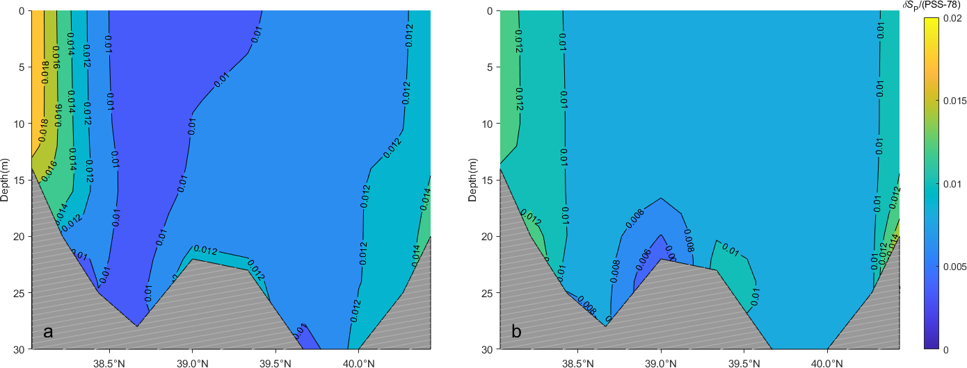
Figure 5 Multi-year mean $\delta S_{\text{P}}$ isolines along Section B with (A) depicting values in winter and (B) in summer.

Both $\delta S_{\text{A}}$ and $\delta S_{\text{P}}$ along Section B are primarily influenced by $\mathrm{\Delta }[{\text{HCO}}_3^{-}]$ and $\mathrm{\Delta }[{\text{Ca}}^{2+}]$ in seawater. The distribution of mean values in winter and summer mirrors that of $\mathrm{\Delta }[{\text{HCO}}_3^{-}]$, with the minimum value occurring in the middle and gradually increasing toward the southwest and northeast ends. In winter, the maximum $\delta S_{\text{A}}$ value of 0.06 g·kg^-1 is observed at the estuary of the Yellow River, while the remainder exceeds 0.01 g·kg^-1. $\delta S_{\text{A}}$ exhibits minimal variation along the vertical axis. Except for the two stations near the estuary of the Yellow River, the differences in $\delta S_{\text{A}}$ between summer and winter were less than 0.01 g·kg^-1 at the remaining eight stations.

Similarly, the maximum $\delta S_{\text{P}}$ value of 0.04 is observed at the two stations at the southwest end of Section B. The remaining stations exhibit $\delta S_{\text{P}}$ values ranging from 0.01 to 0.02.

Feistel et al. (2010) observed significant changes in $\delta S_{\text{A}}$ in the Baltic Sea over the past three decades. Similarly, Ji et al. (2021) noted notably higher $\delta S_{\text{A}}$ values in the Bohai Sea during the winter of 2007 compared to the multi-year average. Considering these findings, it becomes imperative to examine the long-term patterns of $\delta S_{\text{A}}$ and $\delta S_{\text{P}}$ variations. To address this, we selected four stations—B01, B04, B07, and B10—at equal intervals along Section B for investigation. The results are presented in Figure 6 and Table 1.

Figure 6

Figure 6 $\delta S_{\text{A}}$ versus $S_{\text{P}}$ of 4 stations of Section B from 1985 to 2020.

Table 1

Table 1 The multi-year mean $\delta S_{\mathrm{\text{A}}}$ and $\delta S_{\text{P}}$ of the four stations along Section B.

As that Pawlowicz (2015) estimated that the $\delta S_{\text{A}}$ of Yellow River is the largest (about 0.2 g/kg^-1) among rivers flowing into Chinese offshore waters, the $\delta S_{\text{A}}$ values at station B01, situated very close to the estuary of the Yellow River, not only exhibit significantly higher values ranging from 0.02 to 0.1 g·kg^-1 compared to other stations, but also display more pronounced seasonal variations and differences between the bottom and the surface.

Specifically, $\delta S_{\text{A}}$ tends to be higher in winter than in summer, with a more pronounced difference observed between the bottom and the surface layers.

The correlation coefficients between $\delta S_{\text{A}}$ values in summer and winter of the same year hover around 0.1 at all four stations. This suggests that the nutrient and inorganic carbon composition anomalies tend to return to a common state in summer and do not persist into the following year after undergoing water exchange in and out of the Bohai Sea, as well as experiencing geochemical processes and biological consumption throughout the year. Consequently, there is no discernible long-term trend in $\delta S_{\text{A}}$ at station B01.

In contrast, the remaining three stations (B04, B07, and B10) exhibit significantly lower $\delta S_{\text{A}}$ values, with weaker interannual variability and less pronounced seasonal and vertical variability compared to station B01.

The temporal variations of $\delta S_{\text{P}}$ along Section B mirror those of $\delta S_{\text{A}}$. However, the values of $\delta S_{\text{P}}$ are consistently lower, ranging from one-third to one-half of the values observed for $\delta S_{\text{A}}$, with variations typically falling between 0 and 0.04. This discrepancy suggests that $\delta S_{\text{P}}$ exhibits greater stability. This stability observed can be attributed to the relatively minor impact of additional dissolved calcium carbonate on conductivity compared to the predominant solute in seawater NaCl.

These measurements underscore the evident differences in salinity anomalies among various stations, which are intricately linked to factors such as geographic location, water exchange dynamics, and terrestrial inputs. Hence, when investigating salinity changes in the Bohai Sea, it is imperative to thoroughly consider the disparities and influencing factors across different stations.

3.3 Parameterization of $\delta S_{\text{A}}$ and $\delta S_{\text{P}}$ of the Bohai Sea

The absolute salinity ($S_{\text{A}}$) of a seawater sample with the reference salinity ($S_{\text{R}}$) is typically calculated by considering the sample as a mixture composed of a known fraction ($f$) of Standard Seawater (SSW) with a salinity of $S_{\text{SO}}=$ 35.16504, and a fraction of 1- $f$ of river water with a salinity of $S_{\text{RW}}$ (Feistel et al., 2010; Millero, 2013; Pawlowicz, 2015). The equation is as follows:

$\begin{array}{ll}{S}_{\text{A}}=S_{\text{R}}+(1-S_{\text{R}}/S_{\text{SO}})S_{\text{RW}}& (14)\end{array}$

The primary relative compositional anomalies, $\mathrm{\Delta }[{\text{HCO}}_3^{-}]$ and $[{\text{Ca}}^{2+}]$, in Bohai Sea seawater are both higher at the bottom in winter than at the surface in summer. Interestingly, despite most runoffs around the Bohai Sea being discharged into the sea during the summer, suggesting that the Yellow River and other inlet runoff are not the primary sources of these substances, Equations 6 and Equation 14 cannot be applied for calculating the $\delta S_{\text{A}}$ of the Bohai Sea.

Strong northward winds prevalent in the Bohai Sea during winter not only contribute to sediment suspension and re-solubilization (Zhang et al., 1995; Hong, 2012) but also facilitate the exchange of seawater between the Bohai and Yellow Seas (Chen, 1992; Ju et al., 2020). To investigate whether a significant trend or pattern exists in the influence of winter winds on $\mathit{\delta }{\mathit{S}}_{\mathit{A}}$ in the Bohai Sea, correlation analyses between the sea surface 10-meter high wind speeds from ERA5 and $\mathit{\delta }{\mathit{S}}_{\mathit{A}}$ at four stations (B01, B04, B07, and B10) in February (the month of the winter section survey) from 1985 to 2020 were conducted. Firstly, the winter wind speed series and $\mathit{\delta }{\mathit{S}}_{\mathit{A}}$ series were normalized using the following equation: demonstrate the application of Equation (15).

$\begin{array}{ll}Y=\frac{(X-\text{mean}(X))}{\text{std}(X)}, X= \left\{x_{1985,}{x}_{1986,\cdots ,}{x}_{2020}\right\}& (15)\end{array}$

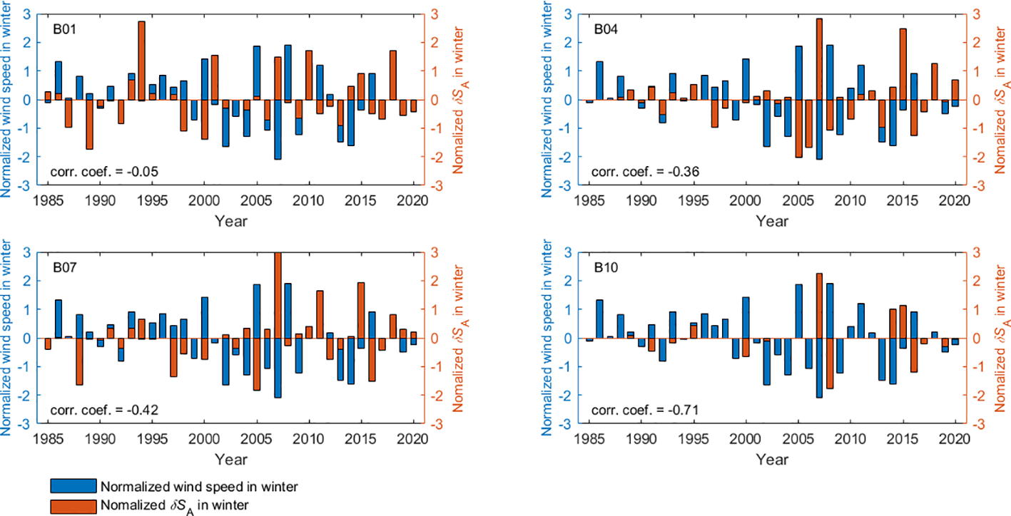
Subsequently, the correlation coefficients between the normalized wind speed serial and normalized $\mathbf{\delta }{\mathbf{S}}_{\mathbf{A}}$ serial at each station were calculated for the winter from 1985 to 2020, the results are illustrated in Figure 7.

Figure 7

Figure 7 Normalized $\delta S_{\text{A}}$ versus normalized averaged wind speed of 4 stations of Section B in winter from 1985 to 2020.

As depicted in Figure 7, there is a moderate negative correlation between winter $\delta S_{\text{A}}$($\delta S_{\text{A}\_\text{winter}}$) and the average winter wind speed along section B. Consequently, in years when the $\delta S_{\text{A}\_\text{winter}}$ value reaches an extreme, winter winds are milder than average, and local geochemical processes exert a greater influence on $\delta S_{\text{A}\_\text{winter}}$ than winter water exchange does.

Based on the source and seasonal variation of relative composition anomalies, the equations for $\delta S_{\text{A}}$ and $\delta S_{\text{P}}$ in the Bohai Sea can be fitted using measurements from Section B as follows:

$\begin{array}{ll}\begin{array}{c}\delta S_{\text{A}}=\delta S_{\text{A}}(\Phi ,\lambda ,Summer/Winter)\\ \delta S_{\text{P}}=\delta S_{\text{P}}(\Phi ,\lambda ,Summer/Winter)\end{array}\}& (16)\end{array}$

In which $\Phi$ is the latitude, $\lambda$ is the longitude. The $\delta S_{\text{A}}$ and the $\delta S_{\text{P}}$ of the four stations of Section B are listed in Table 1. Note that due to the lack of measured data, Equation 16 only applies to data obtained in the Bohai Sea in summer or winter.

Due to limited publicly available data, the $\delta S_{\text{A}}$ function in the current release of the TEOS-10 library, GSW3.07, is only linearly extrapolated from the deep ocean to the offshore, taking into account only non-conducting silicates. This results in a $\delta S_{\text{A}}$ value of only 0.002 g·kg^-1 (Ji et al., 2021). In contrast, the $\delta S_{\text{A}}$ obtained from Equation 16 ranges from 0.02 to 0.1 g·kg^-1 with an uncertainty order of magnitude between 0.007 and 0.021 g·kg^-1. Thus, it significantly enhances the accuracy of calculating the thermodynamic properties of seawater in the Bohai Sea.

As conventional physical oceanographic surveys often lack comprehensive water chemistry measurements, Equation 16 can be easily and swiftly applied to calculate $S_{\text{A}}$ at stations near the section, thereby improving the accuracy of determining the thermodynamic properties of Bohai seawater. For studies still employing $S_{\text{P}}$ as a salinity parameter, Equation 16 can elucidate the uncertainty and compatibility level at relevant stations.

4 Discussion and conclusion

Based on marine chemical and physical oceanographic measurements, we observed that the proportion of $[{\text{HCO}}_3^{-}]$ and $[{\text{Ca}}^{2+}]$ ions in the dissolved composition of Bohai Seawater significantly exceeded that of Standard Seawater (SSW). This disparity was primarily attributed to input from terrestrial runoff and the re-dissolution of bottom sediments. The Bohai Sea, characterized by a narrow mouth and expansive basin, experiences typical monsoon climate conditions. Consequently, its water movement, runoff inputs, and biogeochemical processes exhibit strong seasonal characteristics, leading to seasonal fluctuations in compositional anomalies without obvious time-accumulation effects. This contrasts with the dissolved composition anomaly of the Baltic Sea, where terrestrial runoff inputs predominantly influence composition, accompanied by significant time-accumulation effects.

Utilizing the distinct spatial and temporal variations of dissolved constituent anomalies in Bohai Sea water, we have successfully derived an empirical formula for $\delta S_{\text{A}}$ of the Bohai Sea, elucidating the corresponding uncertainty magnitude. These findings provide valuable insights for accurately calculating the thermodynamic parameters of Bohai Sea water, including density, heat capacity, sound velocity, reflection coefficient, refractive index, and viscosity. This enhanced understanding facilitates a deeper comprehension of the unique hydrological characteristics specific to the Bohai Sea.

The precise characterization of salinity in semi-enclosed sea areas holds particular importance, as changes in salinity coincide with alterations in seawater density, subsequently impacting the intensity and direction of ocean currents, ultimately influencing local sea level height. Moreover, salinity fluctuations can significantly impact the composition, growth rate, competitive dynamics, and nutrient cycling of algal communities, exerting a profound influence on the stability and functionality of entire ecosystems. Therefore, accurately characterizing salinity not only enhances our understanding and predictive capabilities concerning local marine dynamic processes but also holds significant implications for ecosystem protection and management.

Salinity, served as an essential climate variable, plays a pivotal role in ensuring the compatibility of measurements collected from diverse global regions and times, thereby averting misleading trends and discontinuities in climate change assessments. The evolution of seawater salinity measurement methods has been extensive, transitioning from the early technique of drying seawater and weighing residue to the contemporary approach of calculating salinity based on the consistent relative proportion of dissolved substances, determined through chlorinity or conductivity measurements and empirical formulas. Presently, the advancement has led to the determination of absolute salinity by correcting practical salinity. It’s imperative to note that only Absolute Salinity can accurately represent the total mass of dissolved inorganic substances in seawater; all other salinity measurements entail a certain degree of error. To compatible with historical salinity data derived from seawater samples, the calculation of practical salinity has to adhere to proportionality with the chlorine content of these samples and is not be the optimal choice for reflecting the mass fraction of dissolved substances in seawater samples, potentially introducing errors in calculated parameters such as seawater density or gradient flow. Moreover, deviations may arise between practical salinity and chlorinity-derived salinity when the relative composition of seawater diverges from standard seawater (SSW). In Bohai Sea waters, this discrepancy can be as high as 0.04 (PSS-78), with the disparity from absolute salinity reaching a maximum of 0.1 g·kg^-1. This discrepancy arises primarily because the predominant components of Bohai Sea water, namely $[{\text{HCO}}_3^{-}]$ and $[{\text{Ca}}^{2+}]$, have a significantly smaller impact on conductivity compared to the same mass of NaCl, the main solute in seawater. As a result, the resulting $\delta S_{\text{A}}$ values attributed to these constituents are two to three times greater than those of $\delta S_{\text{P}}$.

Assuming that small changes in the relative dissolved constituents of Bohai Sea water are ignored, the level of compatibility of practical salinity is higher than the level of compatibility of absolute salinity when analyzing long-term changes in the salinity. Therefore, when utilizing these data for long-term salinity change studies, we need to be prudent and take appropriate measures to ensure the accuracy and reliability of the findings.

This study leverages extensive oceanographic data to compute salinity anomalies and their associated uncertainties resulting from specific geochemical processes. However, given the incomplete understanding of the precise chemical composition of Bohai Sea seawater, it’s crucial to carefully consider other potential unknown components, such as the potential impact of changes in sulfate content. Additionally, it’s worth noting that these research findings may have certain limitations when addressing changes in seawater chemical composition caused by various processes.

Moreover, the discontinuity of observation data in both time and space may hinder our ability to achieve a comprehensive analysis of local or specific time periods of seawater changes, thereby restricting our thorough understanding of complex systems or phenomena. Therefore, there’s a pressing need to enhance the accuracy of the calculation formula for absolute salinity in nearshore or semi-enclosed waters due to insufficient observation data. To more accurately elucidate the essence of this complex phenomenon, obtaining more direct measurement data and other relevant information is urgently required.

Data availability statement

The research data used in this manuscript have not been publicly available yet because the investigators are still conducting relevant research based on these massive data. At present, the relevant atlas and research reports have been officially published and listed in the references list: (1)State Ocean Administration of China. China Offshore Atlas – Ocean Chemistry. Ocean Press, Beijing, 2016, ISBN: 978-7-5027-9416-3. (2)State Ocean Administration of China. China Offshore Atlas – Oceanography. Ocean Press, Beijing, 2016. ISBN: 978-7-5027-8394-5 Researchers interested in the data of this study are encouraged to contact the corresponding author at: yangjinkun@nmdis.org.cn.

Author contributions

FJ: Conceptualization, Writing – original draft, Writing – review & editing. JY: Funding acquisition, Writing – review & editing. FD: Data curation, Writing – review & editing. BZ: Data curation, Writing – review & editing. PN: Visualization, Writing – review & editing.

Funding

The author(s) declare financial support was received for the research, authorship, and/or publication of this article. This work was supported by the National Key Research and Development Program of China (Grant No. 2022YFC2806601).

Acknowledgments

We are very grateful to Dr.Jia Jianjun of East China Normal University for his valuable discussion on this paper.

Conflict of interest

The authors declare that the research was conducted in the absence of any commercial or financial relationships that could be construed as a potential conflict of interest.

Publisher’s note

All claims expressed in this article are solely those of the authors and do not necessarily represent those of their affiliated organizations, or those of the publisher, the editors and the reviewers. Any product that may be evaluated in this article, or claim that may be made by its manufacturer, is not guaranteed or endorsed by the publisher.

References

Chen C. (2009). Chemical and physical fronts in the Bohai, Yellow and East China seas. J. Mar. Syst. 78, 394–410. doi: 10.1016/j.jmarsys.2008.11.016

CrossRef Full Text | Google Scholar

Chen D. (1992). Marine atlas of bohai sea, yellow sea, east China sea, hydrology (Beijing: China Ocean Press)ISBN:978–7-5027–0904-4.

Google Scholar

Fan W., Xiang W., Wang H. (2021). China oceanographic hydrological and climatological records: bohai volume (Beijing: Ocean Press)ISBN:978–7-5210–0699-5.

Google Scholar

Feistel R. (2008). A Gibbs Function for seawater thermodynamics for 6 to 80°C and salinity up to 120 g kg^-1. Deep Sea Res. I 55, 1619–1671. doi: 10.1016/j.dsr.2008.07.004

CrossRef Full Text | Google Scholar

Feistel R., Weinreben S., Wolf H., Seitz S., Spitzer P., Adel B., et al. (2010). Density and absolute salinity of the baltic sea 2006–2009. Ocean Sci. 6, 3–24. doi: 10.5194/os-6-3-2010

CrossRef Full Text | Google Scholar

Feistel R., Wielgosz R., Bell S., Camões M., Cooper J., Dexter P., et al. (2016). Metrological challenges for measures of key climatic measurements: oceanic salinity and pH, and atmospheric humidity Part 1: Overview. Metrology 53, R1–R11. doi: 10.1088/0026-1394/53/1/R1

CrossRef Full Text | Google Scholar

GCOS (2010). Implementation Plan for the Global Observing System for Climate in support of the UNFCCC (Geneva: World Meteorological Organization), 180. Available at: www.wmo.int/pages/prog/gcos/Publications/gcos-138.pdf. WMO-TD/No. 1532 (GCOS-138).

Google Scholar

Hong H. S. (2012). China regional oceanography – chemical oceanography (Beijing: Ocean Press)ISBN:978–7-5027–8257-3.

Google Scholar

IOC, SCOR, IAPSO (2010). “The international thermodynamic equation of seawater – 2010: calculation and use of thermodynamic properties,” in Manual and guides no. 56, intergovernmental oceanographic commission (UNESCO) Printed by UNESCO, Paris.

Google Scholar

Ji W. (2016). China offshore oceans marine chemistry (Beijing: Ocean Press), ISBN: ISBN: 978–7-5027–8259-7.

Google Scholar

Ji F., Pawlowicz R., Xiong X. (2021). Estimating the Absolute Salinity of Chinese offshore waters using nutrients and inorganic carbon data. Ocean Sci. 17, 909–918. doi: 10.5194/os-17-909-2021

CrossRef Full Text | Google Scholar

Ju X., Ma C., Yao Z., Bao X. (2020). Case analysis of water exchange between the Bohai and Yellow Seas in response to high winds in winter. J. Oceanology Limnology 38, 30–41. doi: 10.1007/s00343-019-9100-2

CrossRef Full Text | Google Scholar

Le Menn M. (2011). About uncertainties in practical salinity calculations. Ocean Sci. 7, 651–659. doi: 10.5194/os-7-651-2011

CrossRef Full Text | Google Scholar

Lewis E., Wallace D. (1998) Program developed for CO2 system calculations (Github). Available online at: https://github.com/jamesorr/CO2SYS-MATLAB (Accessed 8 June 2021).

Google Scholar

Li A. (2016). Interannual variations of yellow sea cold water mass, phD dissertation (Qingdao: Graduate School of the Chinese Academy of Sciences Institute of Oceanology).

Google Scholar

Lin C., Su J., Xu B. (2001). Long term variations of temperature and salinity of the Bohai Sea and their influence on its ecosystem. J. Prog. Oceanography 49, 7–19. doi: 10.1016/S0079-6611(01)00013-1

CrossRef Full Text | Google Scholar

Luo C., Lin L., Shi J., Liu Z., Cai Z., Guo X., et al. (2021). Seasonal variations in the water residence time in the Bohai Sea using 3D hydrodynamic model study and the attachment method. Ocean Dynamics 71, 157–173. doi: 10.1007/s10236-020-01438-5

CrossRef Full Text | Google Scholar

Lv C. (2008). Analysis of decadal variability of salinity field and its influence to circulation in Bohai and northern Yellow Sea (Qingdao: The Master Degree Dissertation of China Ocean University).

Google Scholar

Ma C., Wu D., Lin X. (2006). The interannual and long term variation characteristics and causes of salinity in the Bohai Sea and the Yellow Sea. J. Ocean Univ. China Natural Sci. Edition 36, 7–12.

Google Scholar

McDougall T. J., Barker P. (2011). Getting started with TEOS-10 and the gibbs seawater (GSW) oceanographic toolbox. 28ISBN: 978–0-646–55621-5, SCOR/IAPSO WG127. Available at: www.TEOS-10.org

Google Scholar

McDougall T., Jackett D., Millero F., Pawlowicz R., Barker P. (2012). A global algorithm for estimating Absolute Salinity. Ocean Sci. 8, 1123–1134. doi: 10.5194/os-8-1123-2012

CrossRef Full Text | Google Scholar

Millero F. (2013). Chemical oceanography. 4th ed. (CRC press).

Google Scholar

Millero F., Feistel R., Wright D., McDougall T. (2008). The composition of Standard Seawater and the definition of the Reference-Composition Salinity Scale. Deep-Sea Res. Pt. I 55, 50–72. doi: 10.1016/j.dsr.2007.10.001

CrossRef Full Text | Google Scholar

Pawlowicz R. (2008). Calculating the conductivity of natural waters. Limnol. Oceanogr.: Methods 6, 489–501. doi: 10.4319/lom.2008.6.489

CrossRef Full Text | Google Scholar

Pawlowicz R. (2010). A model for predicting changes in the electrical conductivity, practical salinity, and absolute salinity of seawater due to variations in relative chemical composition. Ocean Sci. 6, 361–378. doi: 10.5194/os-6-361-2010

CrossRef Full Text | Google Scholar

Pawlowicz R. (2015). The Absolute Salinity of seawater diluted by river water. Deep-Sea Res. Pt. I 101, 71–79. doi: 10.1016/j.dsr.2015.03.006

CrossRef Full Text | Google Scholar

Pawlowicz R., Feistel R., McDougall T. J., Ridout P., Seitz S., Wolf H. (2016). Metrological challenges for measures of key climatic observables - Part 2: Ocean salinity. Metrology 53, R12–R15. doi: 10.1088/0026-1394/53/1/R12

CrossRef Full Text | Google Scholar

Pawlowicz R., Wright D., Millero F. (2011). The effects of biogeochemical processes on oceanic conductivity/salinity/density relationships and the characterization of real seawater. Ocean Sci. 7, 363–387. doi: 10.5194/os-7-363-2011

CrossRef Full Text | Google Scholar

Qi D. (2013). Dissolved calcium in the yangtze river estuary and China offshore (The Master Degree Dissertation of Xiamen University) Xiamen University Press: Xiamen.

Google Scholar

Seitz S., Feistel R., Wright D., Weinreben S., Spitzer P., de Bievre P. (2011). Metrological traceability of oceanographic salinity measurement results. Ocean Sci. 7, 45–62. doi: 10.5194/os-7-45-2011

CrossRef Full Text | Google Scholar

Uchida H., Kawano T., Nakano T., Wakita M., Tanaka T., Tanihara S. (2020). An expanded batch-to-batch correction for IAPSO standard seawater. J. Atmos. Oceanic Technol. 37, 1507–1520. doi: 10.1175/JTECH-D-19-0184.1

CrossRef Full Text | Google Scholar

UNESCO (1981). The practical salinity scale 1978 and the international equation of state of seawater 1980. UNESCO Tech. Papers Mar. Sci. 36, 25.

Google Scholar

Woosley R., Huang F., Millero F. (2014). Estimating absolute salinity (SA) in the world’s oceans using density and composition. Deep Sea Res. I 93, 14–20. doi: 10.1016/j.dsr.2014.07.009

CrossRef Full Text | Google Scholar

Xing F., Sun J., Li Y., Yuan, Tao J. (2013). “Numerical simulation of water exchange in bohai sea with age and half-life time,” in Proceedings of 2013 IAHR world congress. Tsinghua University Press: Beijing.

Google Scholar

Xiong X. (2012). China offshore oceans—Physical oceanography and marine meteorology (Beijing: Ocean Press), ISBN: ISBN:978–7-5027–8247-4.

Google Scholar

Xu J. (2007). The variation characters and formation mechanism of salinity in the bohai sea (Qingdao: Ocean University of China, Master Thesis).

Google Scholar

Yu H., Bao X., Lü C., Chen X., Kuang L. (2009). Analyses of the long-term salinity variability in the Bohai Sea and the northern Huanghai(Yellow)Sea. Acta Oceanologica Sin. 28, 1–8.

Google Scholar

Yu F., Zhang Z., Diao X., Guo J., Tang Y. (2006). Analysis of the evolution process of cold water masses in the Yellow Sea and their relationship with neighbouring water masses. J. Oceanography 28, 26–34. doi: 10.3321/j.issn:0253–4193.2006.05.003

CrossRef Full Text | Google Scholar

Zhang J., Huang W. W., Létolle R., Jusserand C. (1995). Major element chemistry of the Huanghe River (Yellow River), China weathering processes and chemical fluxes. J. Hydrol. 168, 173–203. doi: 10.1016/0022-1694(94)02635-O

CrossRef Full Text | Google Scholar

Zhang Z., Qiao F., Guo J., Guo B. (2018). Seasonal changes and driving forces of inflow and outflow through the Bohai Strait. Continental Shelf Res. 154, 1–8. doi: 10.1016/j.csr.2017.12.012

CrossRef Full Text | Google Scholar

Zweng M. M., Reagan J. R., Seidov D., Boyer T. P., Locarnini R. A., Garcia H. E., et al. (2019). World ocean atlas 2018, volume 2: salinity Vol. 82. Ed. Mishonov A. (Silver Spring, Maryland: NOAA Atlas NESDIS), 50. doi: 10.25923/54bh-1613

CrossRef Full Text | Google Scholar