Image stitching and target perception for Autonomous Underwater Vehicle-collected side-scan sonar images

Introduction: Autonomous Underwater Vehicles (AUVs) are capable of independently performing underwater navigation tasks, with side-scan sonar being a primary tool for underwater detection. The integration of these two technologies enables autonomous monitoring of the marine environment.

Methods: To address the limitations of existing seabed detection methods, such as insufficient robustness and high complexity, this study proposes a comprehensive seabed detection method based on a sliding window technique. Additionally, this study introduces a sonar image stitching method that accounts for variations in image intensity and addresses challenges arising from multi-frame overlaps and gaps. Furthermore, an autonomous target perception framework based on shadow region segmentation is proposed, which not only identifies targets in side-scan sonar images but also provides target height measurements.

Results: Comprehensive seabed detection method improves accuracy by 31.2% compared to the peak detection method. In experiments, the height measurement error for this method was found to be 9%.

Discussion: To validate the effectiveness of the proposed seabed detection method, sonar image stitching method, and target perception framework, comprehensive experiments were conducted in the Qingjiang area of Hubei Province. The results obtained from the lake environment demonstrated the effectiveness of the proposed methods.

1 Introduction

Autonomous underwater vehicles (AUVs) are playing a crucial role in scientific, commercial and military applications (Lin and Yang, 2020). In autonomous marine monitoring systems, AUVs typically serve as platforms carrying side-scan sonar and other sensors for detecting the topography and targets within a designated area. Upon completion of their tasks, they either surface or connect underwater to upload the collected data (Lin et al., 2022; Zhang et al., 2024). Side-scan sonar (SSS) stands out as a primary device for underwater monitoring due to its high resolution, cost-effectiveness, and versatility. Leveraging the principle of echo sounding, side-scan sonar detects underwater topography. With a lower attenuation coefficient in water compared to optical devices, sonar proves superior in seabed detection and finds wide applications across oceans, rivers, lakes, and ports. Current applications span but are not limited to localized marine ecosystem monitoring, aquaculture and endangered species detection, hydrothermal vent and cold seep exploration, underwater search and rescue operations, among others.

The autonomous monitoring system primarily comprises two components: the AUV and the docking station. The AUV departs from the docking station, utilizing its onboard positioning and control systems, along with side-scan sonar, to investigate the topography and targets within a designated area. Upon completing its mission, the AUV reconnects with the docking station underwater, facilitating energy transfer and data transmission. A schematic diagram of the operational process is shown in Figure 1.

Figure 1

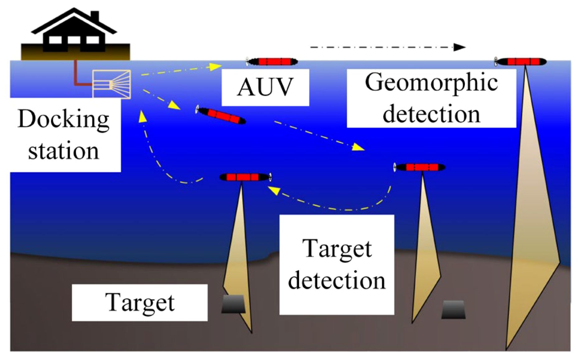
Figure 1 AUV operation diagram.

Equipping the AUV with side-scan sonar enables autonomous seabed exploration, which is crucial for marine ranches. The autonomous exploration of marine ranches encompasses two main aspects:

Topographic Survey: The AUV, equipped with its own positioning sensors and integrated navigation control system, navigates along predetermined paths, serving as a platform for side-scan sonar data acquisition. The positioning system provides global localization, enabling the collection of topographic data from specified areas and the georeferenced stitching of side-scan sonar data, thus facilitating autonomous monitoring.

Target Settlement Monitoring: The AUV can carry an appropriate depth sensor, allowing it to bring the side-scan sonar to a specific depth to detect underwater targets. By employing corresponding side-scan sonar data processing methods, the AUV can perceive underwater targets, addressing the issue of autonomous monitoring within marine ranches.

This comprehensive approach ensures that the AUV can effectively perform autonomous monitoring tasks, enhancing the efficiency and accuracy of marine environmental surveys. This paper investigates the research on image stitching and target perception methods for side-scan sonar images aimed at AUVs. Image stitching and target perception are crucial technologies for long-term monitoring.

Accurately tracking the seabed line from the raw data of side-scan sonar is essential for subsequent processing, such as slant range correction, image stitching, and target perception. Side-scan sonar images exhibit significant grayscale variations at the location of the seabed line, which has led to the development of numerous methods for detecting the seabed line. However, the current traditional seabed line detection methods (Woock, 2011; Ramirez, 2014) suffer from problems such as low robustness and complex processes, while deep learning-based methods require building datasets and have poor model transferability (Zheng et al., 2021; Qin et al., 2022). Therefore, it is necessary to enhance the robustness of seabed line detection methods while considering process complexity. This paper proposes a comprehensive seabed line detection method based on a sliding window approach. This method achieves effective seabed line detection with strong robustness and simplicity, laying a solid foundation for subsequent image stitching and target perception. Finally, the paper performs radiation correction and slant range correction on the images based on the working principles of side-scan sonar.

Due to issues like non-continuous geographic positioning data and inconsistent resolution in the horizontal and vertical directions in the data collected by side-scan sonar, it is necessary to combine global or relative positioning to complete the image stitching of side-scan sonar, reflecting the true distribution of the seafloor topography. Applying optical stitching methods directly to acoustic images leads to problems such as limited feature matching and stitching errors due to the fewer features, low signal-to-noise ratio, and the need for sonar data positioning. Scholars have proposed various solutions to address these problems, mainly divided into feature-based stitching methods (Bay et al., 2006) and transform domain-based stitching methods (Hurtós et al., 2015). However, currently, sonar image stitching mainly focuses on stitching multiple images and does not address the frame-to-frame processing issue during underwater vehicle operation. In the stitching process, the paper derives the coordinate transformation relationship between the carrier coordinate system and the navigation coordinate system, as well as the relevant transformation formulas for geocoding of side-scan sonar images. It also addresses the gap and overlap problems that occur during stitching, achieving autonomous image stitching.

As a crucial device for acquiring underwater information, side-scan sonar has high resolution and can accurately detect underwater targets. AUVs equipped with side-scan sonar can achieve autonomous perception of underwater targets through appropriate methods. However, there is relatively little research on achieving target segmentation from raw side-scan sonar data in scenarios where segmentation is performed simultaneously with data acquisition. Therefore, a feasible method for autonomous detection by AUVs is needed. To enable AUVs equipped with side-scan sonar to autonomously perceive underwater targets, and considering the difficulty of real-time target perception from side-scan sonar data, this paper proposes an autonomous target perception method based on a classification algorithm. First, the effective region image is obtained by utilizing the seabed line detection results. Then, the EfficientNet classification algorithm is used to classify the acquired images into target or non-target categories to save computational resources. Subsequently, non-local means filtering, K-means clustering for shadow regions, and improved Region-Scalable Fitting (RSF) segmentation are applied to the images with targets to achieve accurate segmentation of shadow areas. After obtaining the target region, the target height is analyzed.

The remainder of this paper is organized as follows: In Section 2, we introduce the related work on seabed line detection, sonar image stitching, and sonar image target perception. In Section 3, we discuss the image preprocessing method based on seabed line detection. Section 4 presents the method for stitching side-scan sonar images. Section 5 presents the framework for autonomous target perception from side-scan sonar images. Experimental results in a lake environment are presented in Section 6 to demonstrate the effectiveness of the proposed methods. Finally, conclusions are drawn in Section 7.

2 Related work

In this section, we reviewed the relevant research on seabed observation, sonar image stitching, and sonar image target perception.

2.1 Submarine detection

Side-scan sonar images exhibit distinct grayscale variations at seabed contour positions, leading to the development of numerous methods for seabed contour detection based on this principle, as shown in Table 1. Commercial software like Trion (Ramirez, 2014) employs a thresholding method, where a pixel is deemed part of the seabed contour if the difference between its grayscale value and that of the preceding pixel exceeds a predefined threshold. Enhanced thresholding methods, before detection, utilize median filtering to diminish the impact of speckle noise (Woock, 2011). Although these methods enhance the accuracy of seabed contour detection through filtering techniques, they fundamentally rely on thresholding. The selection of thresholds often demands experienced individuals to tailor them based on real-world scenarios, and their precision diminishes significantly in complex seabed environments. A comprehensive bottom-tracking method for side-scan sonar images in complex measurement environments (Zhao et al., 2017) initially employs peak detection, followed by error segment reduction through methods like data filtering, symmetry assumptions, and continuity assumptions, culminating in seabed contour data acquisition via Kalman filtering. While this method boasts robustness, its overall complexity is high. Another approach, employing semantic segmentation for automatic seabed contour tracking (Zheng et al., 2021), incorporates a symmetry information synthesis module, endowing the model with the ability to consider seabed contour symmetry. Additionally, a one-dimensional neural network-based method (Qin et al., 2022) tracks seabed contours using a pre-trained model. Both these methods necessitate dataset construction and training, with the completeness of the dataset significantly impacting model transferability. Traditional seabed contour detection methods currently suffer from low robustness and complexity issues, while deep learning-based approaches require dataset construction and face challenges in model transferability. Hence, there is a need to enhance the robustness of seabed contour detection methods while balancing complexity.

Table 1

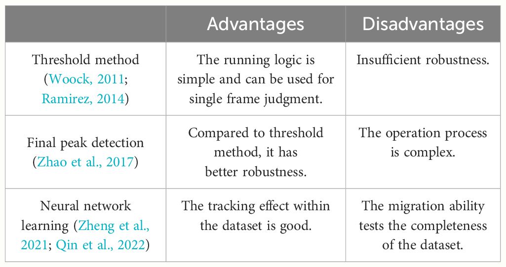
Table 1 Submarine detection method comparison.

2.2 Side scan sonar image stitching method

Scholars have proposed various solutions, primarily categorized into feature-based stitching methods and transformation domain-based stitching methods. Feature-based matching methods involve computing specific features within an image and then matching these features. Commonly used features include SIFT (Lowe, 2003), SURF (Bay et al., 2006), and others. One approach to sonar image stitching, considering the limited number of matching features, utilizes the SURF algorithm in conjunction with trajectory line position constraints (Jianhu et al., 2018), enabling geographic mosaicking in scenarios with insufficient features. Another method (Shang et al., 2021) automatically calculates the overlap region by combining the track line and side-scan sonar image sizes, then segments the overlap region using the K-means method, followed by matching each segmented region using SURF to obtain the stitched image. Transformation domain-based stitching methods involve transforming images into other domains for stitching. One method based on curvelet transformation (Zhang et al., 2021) employs affine transformation to extract and match features, followed by merging the overlapping regions using the curvelet transformation. Another method based on Fourier transformation (Hurtós et al., 2015) registers forward-looking sonar images to address issues such as low resolution, noise, and artifacts. Similarly, another method (Kim et al., 2021) utilizes Fourier transformation to stitch forward-looking sonar images to generate larger-scale images. These methods focus on stitching two complete side-scan sonar images and do not consider the coupled effects between sonar data frames within the same image when deployed on a moving platform like an AUV.

2.3 Target perception method for side scan sonar images

In traditional methods of segmenting side-scan sonar images, techniques such as Fuzzy C-Means clustering (Pal et al., 2005), K-Means clustering (Wong, 1979), level set methods (Ye et al., 2010), active contours (Chenyang and Jerry, 1998), and MRF (Mignotte et al., 1999) are commonly employed. Thresholding involves setting a fixed threshold to categorize pixels above it into one class and those below it into another. An enhanced Fuzzy C-Means clustering method (Abu and Diamant, 2019) accurately segments shadow regions by initially applying a smoothing filter to the image before clustering. The Region-Scalable Fitting (RSF) method (Li et al., 2008), based on the level set theory and minimizing fitting energy, provides a loss function that iteratively approaches the target boundary, resulting in precise segmentation. However, this method is greatly influenced by the initial contour and image quality. A fast and robust side-scan sonar image segmentation algorithm (Huo et al., 2016), building upon the RSF method, integrates K-Means clustering and NLMSF filtering. It employs the results of K-Means clustering as the initial contours for RSF iteration, significantly enhancing both speed and accuracy. Currently, traditional sonar image perception methods focus on segmenting localized regions with known existing targets. However, there is relatively limited research on segmenting targets directly from raw side-scan sonar data in scenarios involving simultaneous data collection and segmentation. Target perception methods that rely heavily on deep learning poses challenges such as dataset creation, extensive labeling, and poor generalization. Therefore, there is a need for a feasible method suitable for autonomous detection by AUVs.

3 Side scan sonar image preprocessing

This study focuses on preprocessing sonar images, stitching together images with geographic information, and calibrating target detection for the autonomous detection of AUVs equipped with side-scan sonar. The entire workflow is illustrated in Figure 2. Figure 2 illustrates the entirety of our study. Figure 2A depicts the scene where an AUV equipped with side-scan sonar operates. During AUV cruising, the side-scan sonar scans the target area. Figure 2B shows the preprocessing steps of the side-scan sonar images. Initially, seabed line detection is conducted, followed by Radiation correction and Slant range correction. These processes are detailed in Section 3. Figure 2C displays the image stitching of each frame of side-scan sonar images. Our focus is on handling gaps and overlaps between frames, a topic elaborated in Section 4. Figure 2D illustrates target detection and height analysis within the side-scan sonar images, which is extensively discussed in Section 5. The following sections introduce each component of the process.

Figure 2

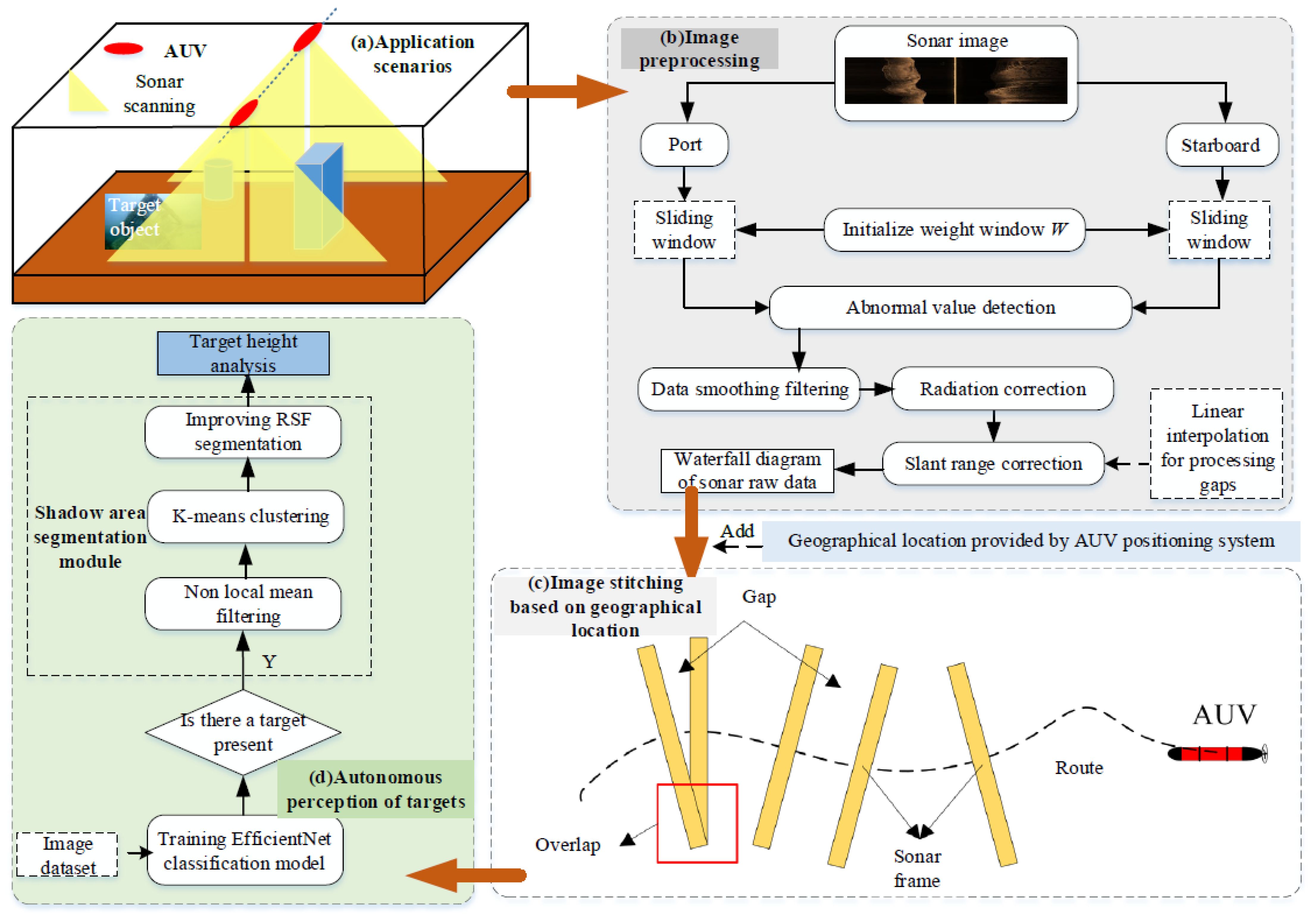
Figure 2 (A–D) The overall workflow of this study.

3.1 Submarine detection

Based on the imaging principle of side-scan sonar and the actual echo intensity of sonar images, it can be observed that the absence of strong reflective objects between the transducer and the seabed results in low echo intensity in that area, forming a dark zone. The boundary of the dark zone, away from the transmission line, represents the seabed line, indicating variations in height from the transducer to the seabed. The seabed line is essential for radiation correction and slant range correction; thus, precise detection of the seabed line is crucial.

To address the shortcomings of existing seabed line detection methods, such as insufficient robustness or complexity, we propose a comprehensive seabed line detection method based on a sliding window approach. This method enables adaptable seabed line detection to complex real-world environments while maintaining computational simplicity.

Considering the limitations of thresholding and peak detection methods, the sliding window approach employs a window with a certain width, enhancing its capability to resist interference with considerable width. The specific expression for window weighting is illustrated in below, where n represents the window width and can be chosen according to requirements, thereby increasing the field of view width.

$$W={[w_1, w_2,\dots , w_n]}_{1\times n}$$

The sonar data window centered on the y-th frame and the i-th pixel on the starboard side can be represented as F, as follows:

$$F={[f(x_{i-left}, y),\dots ,f(x_i, y),\dots , f(x_{i+right}, y)]}_{1\times n}$$

where f(x, y) represents the pixel intensity of the sonar image at (x, y), and n = left + right + 1. Then the weighted sum of the data window can be obtained, as shown below:

$$g(x_i, y)=W{F}^T$$

where g(x_i, y) reflects the disparity in sonar echo intensity between the left and right sides of the data point. The larger the value, the more likely the current data point is to be a seabed line point. Therefore, the point with the maximum weighting sum g(x_i, y) within the data frame is determined as the seabed line point for that frame.

In contrast to thresholding and peak detection methods, the sliding window approach eliminates the need for manually setting a stop threshold. Additionally, the window weight W is an n-dimensional first-order matrix with a certain field of view width, resulting in lower levels of human intervention and increased robustness.

Based on the characteristics of the sliding window approach and the features of side-scan sonar images, a comprehensive seabed line detection method is constructed with the sliding window approach as its foundation. The specific workflow is depicted in Figure 2B.

After performing seabed line detection separately on the left and right sonar images using the sliding window approach, further refinement of the detected data is conducted through outlier detection methods. Subsequently, a data smoothing filter is applied to the final dataset. Regarding outlier detection, it is assumed that the seafloor terrain exhibits continuous variations. Leveraging statistical methods, the seabed line data detected by the sliding window approach is assumed to be represented as follows:

$$S={[s_1, s_2,\dots , s_m]}_{1\times m}$$

where S is the seabed detection result matrix, and m is the height of the side scan sonar image. The block size selected for each outlier detection is (2 × l + 1), so the data block used to detect whether the data s_i is an outlier is:

$$S_k={[s_{i-l}, s_{i-l+1},\dots ,s_i,\dots ,s_{i+l-1},s_{i+l}]}_{1\times (2l+1)}$$

Sorting S_k yields:

$$S_k^{\text{'}}=[{\mathrm{s\text{'}}}_0^{ }, {\mathrm{s\text{'}}}_1^{ },\dots ,{\mathrm{s\text{'}}}_{2l}^{ }]$$

Calculate the average u and variance t of all data in S_k, excluding one maximum and one minimum value:

$$u=\frac{1}{2l-1}{\displaystyle \sum _{j=1}^{2l-1}}{s}_j^{\prime }$$

The criteria for determining outliers are:

$$|s_i-u|>t$$

where if s_i is determined to be an outlier, temporarily correct it using the median in data block S_k and record the corresponding anomaly flag “Flag”, represented as

$$Flag=[f{l}_1,f{l}_2,\cdots ,f{l}_m]$$

Finally, the sliding average method is used to perform a simple filtering on the obtained detection results, resulting in smooth data. To achieve filtering, the window size for filtering is set to (2 × k + 1), and the specific design is as follows:

$$s_i=\frac{1}{P}{\displaystyle \sum _{j=i-k}^{i+k}{s}_j{p}_j}$$

$$P={\displaystyle \sum _{j=i-k}^{i+k}{p}_j}$$

where p_j is the weight, designed based on the distance from the detection point. Points closer to the detection point have a greater weight, while those closer to the detection point have a smaller weight. Here, it is defined as follows:

$$p_j=-a{(i-j)}^2+b$$

It can be seen that p_j decreases with the increase of distance i from j, and both a and b are normal numbers.

3.2 Algorithm comparison

To validate the effectiveness of the comprehensive seabed detection method based on the sliding window technique, corresponding pool experiments were conducted. The experiment utilized the HaiZhuo Tongchuang ES1000 side-scan sonar, mounted on an Autonomous Underwater Vehicle (AUV), operating at a frequency of 900kHz, with a maximum slant range of 75m, a horizontal beamwidth of 0.2 degrees, and a vertical track resolution of 1cm.

During the experiment, the AUV’s propeller speed was controlled by the AUV’s onboard computer, instructing it to move slowly in the pool. The relevant parameters of the side-scan sonar were set, with the maximum slant range defined as 75m. The echo data from the side-scan sonar was transmitted to the main computer on the AUV using TCP communication and stored in xtf format. The actual detection results of the peak detection method and the sliding window method are shown in Figure 3.

Figure 3

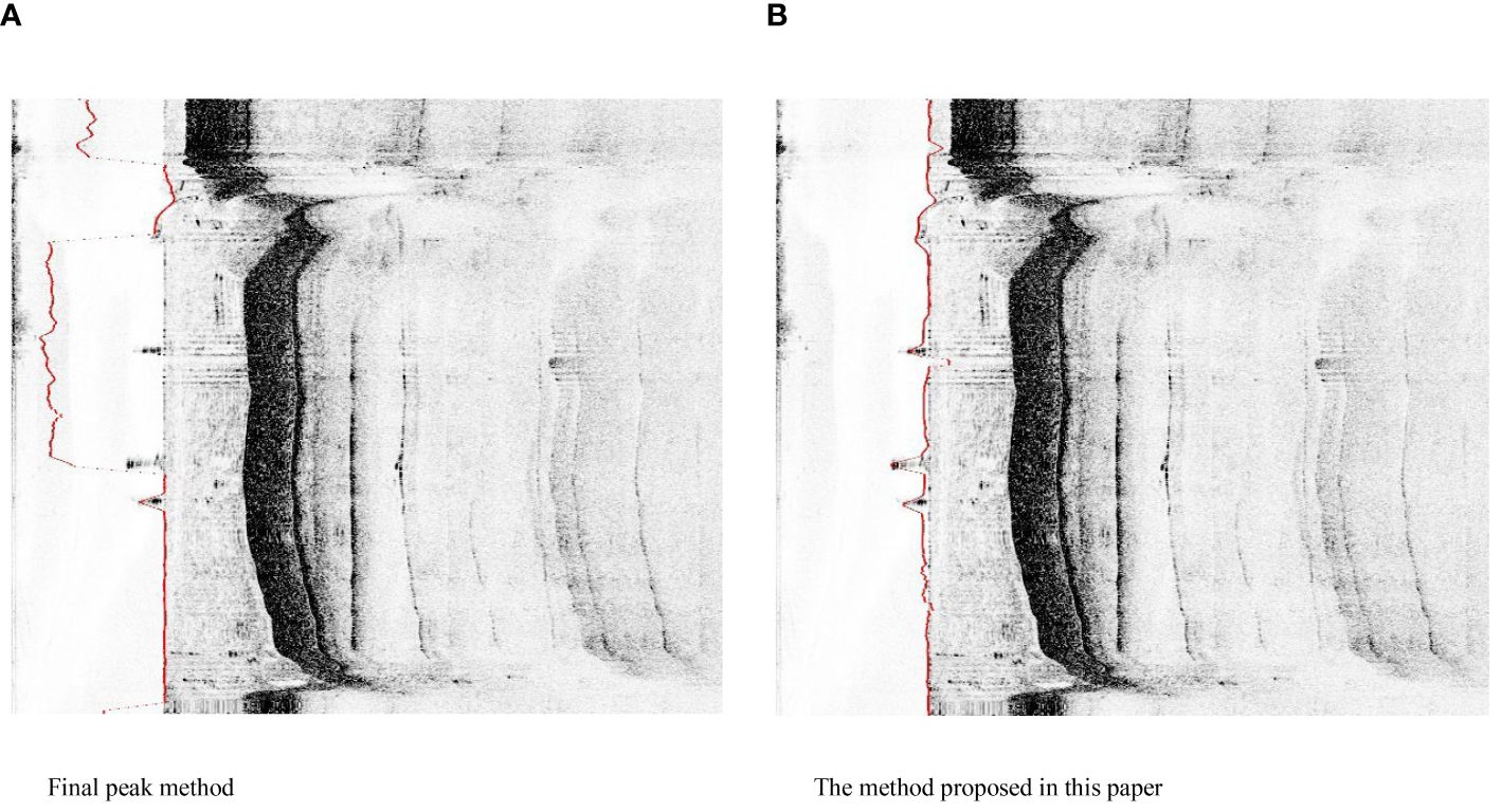
Figure 3 Pool experiment actual test effect. (A) Final peak method. (B) The method proposed in this paper.

In Figure 3, the red dots represent the detected seabed lines. It can be observed that the peak detection method deviates from the true seabed line in some cases due to the influence of noise, while the sliding window method does not exhibit this behavior. Therefore, the sliding window method is more robust against noise interference compared to the peak detection method, and it can accurately track the seabed line even in the presence of noise.

To quantitatively evaluate the two methods’ detection results, a quantitative analysis was performed. Based on the resolution of the side-scan sonar slant range image (each pixel representing 1.4cm * 1.4cm) and considering the pool bottom as a processed flat cement surface, a tape measure was used to measure the water depth during the experiment, which was determined to be 5.36m.

To compare the detection results of the two methods quantitatively, the average values and error rates of the two methods were calculated, as shown in Table 2.

Table 2

Table 2 Comparison result.

It can be seen that the sliding window method proposed in this study yielded an average measurement of 5.276m. Compared to the peak detection method, it exhibited higher accuracy and stronger robustness, with an accuracy improvement of 31.2%.

3.3 Overall processing process.

Given that side-scan sonar displays topographic images, it is desirable to achieve uniform brightness across distances. In practice, as sound waves propagate in water, they incur increased loss with distance, resulting in reduced brightness at the far end of the transmission line on the image. Additionally, the intensity of echoes obtained by side-scan sonar is influenced by seabed media type, roughness, and the grazing angle of sound waves. While modern side-scan sonar equipment incorporates its own Time-Variant Gain (TVG) adjustment, it still necessitates some degree of radiometric correction due to discrepancies between TVG compensation and actual attenuation. Following the attenuation pattern of sound waves, a method employing Mean Amplitude Gain Compensation is utilized for radiometric correction of sonar images.

According to the data acquisition principle of side-scan sonar, the position of the echo is determined by the time it takes for the sound wave to return. Consequently, in the raw data of side-scan sonar, the position is determined by slant range, not the horizontal distance between the detection point and the transducer. Additionally, due to the aforementioned reasons, the topographic image in the vertical direction is compressed, with the compression becoming more severe closer to the transducer and less noticeable farther away. Therefore, to eliminate invalid data from the dark area before the seabed line and reflect the true topographic conditions of the detected area, appropriate slant range correction is required for the original image. The geometric schematic of slant range correction is illustrated in Figure 4.

Figure 4

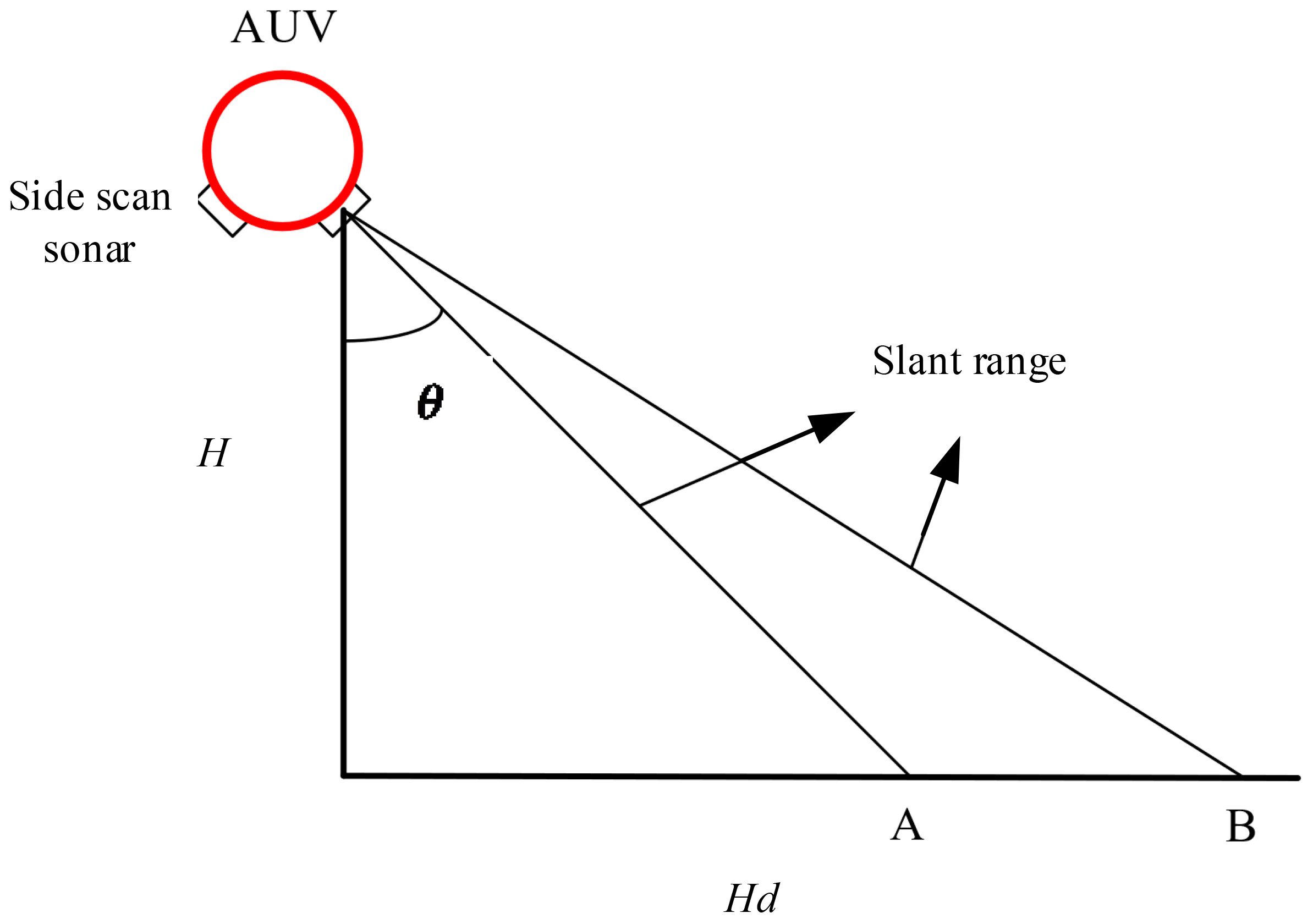
Figure 4 Geometric diagram of oblique range correction.

From the geometric relationship, it can be seen that the oblique range and flat range recorded in sonar images form a right-angled triangle with the ground clearance height. The following calculation and inference will be based on the starboard image.

$$Hd=\sqrt{S_r^2+H^2}$$

$$S_r=y{R}_r$$

where Hd is the horizontal distance from the pixel to the transducer, S_r is the oblique distance from the pixel to the transducer, H is the height of the transducer from the seabed, R_r is the horizontal resolution of the side scan sonar image, and y is the vertical coordinate of the current pixel. In addition, based on the seabed detection results, it can be obtained that:

$$H=s{R}_r$$

where s is the ordinate of the detected seabed line point. Therefore, the specific calculation expression for the horizontal distance Hd can be derived as:

$$Hd=R_r\sqrt{y^2+s^2}$$

Slant range correction restores the compression that originally existed, thus resulting in corresponding gaps after the correction. Addressing the gaps between frames, considering the correlation of data within sonar frames, linear interpolation is contemplated as a method for filling them.

Assuming two horizontally adjacent pixel points before slant range correction are denoted as $f(x, y)$ and $f(x, y+1)$, and their coordinates after correction become $(x, y^{\prime })$ and $(x, y^{\prime }+\Delta y)$ respectively, the intensity of the pixel located between these two points can be calculated as follows:

$$f(x,y^{\prime }+a)=f(x,y^{\prime })+a\ast \frac{(f(x,y^{\prime })-f(x,y^{\prime }+\Delta y))}{\Delta y}$$

where $a<\Delta y$.

Based on the aforementioned explanation, the basic process of preprocessing side-scan sonar images is completed, laying a certain foundation for subsequent tasks such as image stitching and target perception. The overall processing process is shown in the Figure 5.

Figure 5

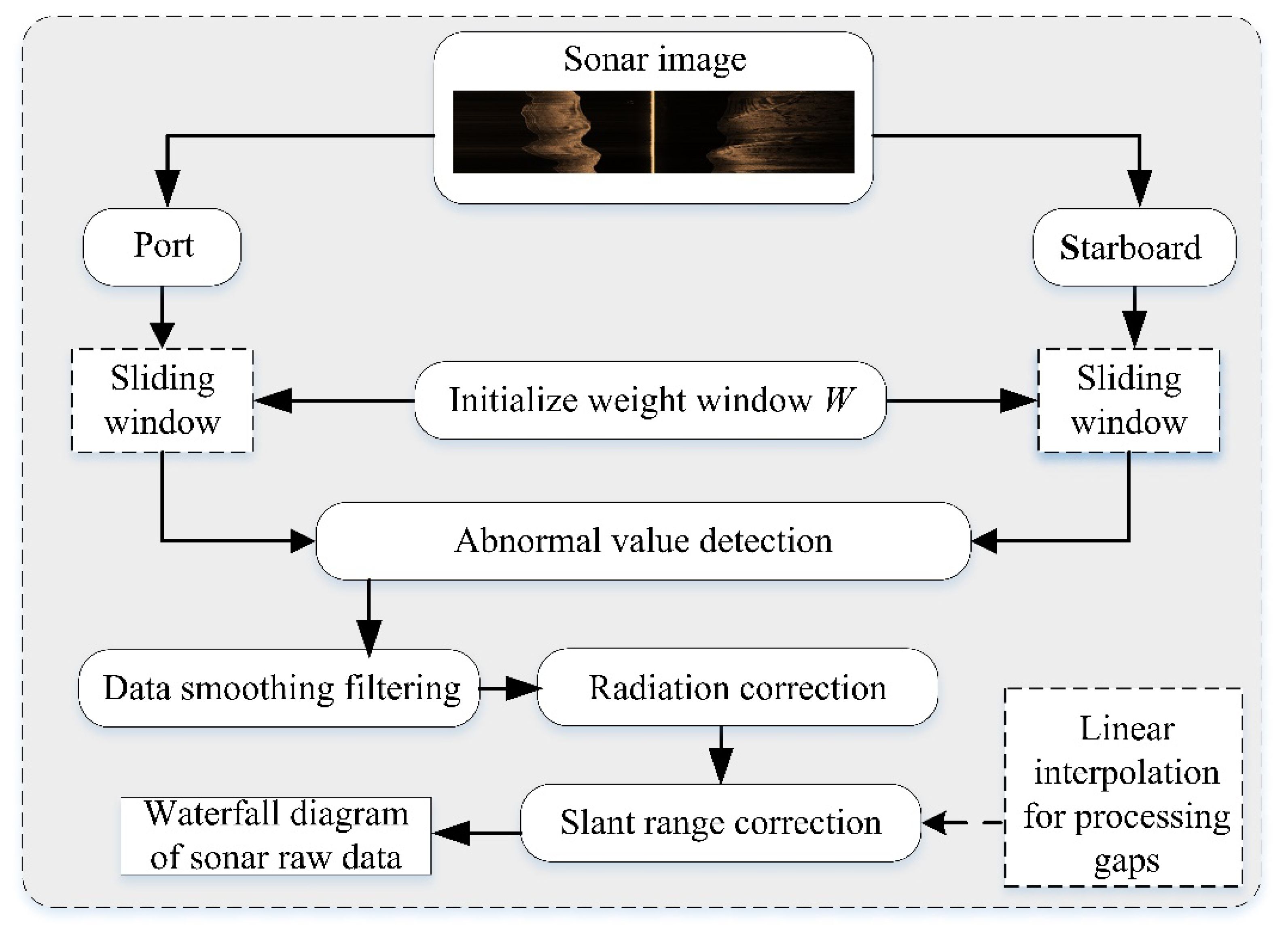
Figure 5 The overall processing process.

4 Image stitching containing geographic information during AUV navigation

Detecting seabed topography is a crucial aspect of environmental monitoring. After preprocessing the raw side-scan sonar data, as described in the previous section, we obtain effective data on the seabed topography scanned by the side-scan sonar. However, to achieve complete and coherent mapping, it is necessary to integrate this data with actual positioning and heading information in order to stitch together each frame of the sonar images accurately.

4.1 Geocoding

In Section 3, seabed line detection, radiometric correction, and slant range correction of side-scan sonar images were conducted. These steps allow for obtaining effective data from side-scan sonar and the actual relative positions of individual sonar frames. However, the relative positions between frames still need to be determined. Therefore, the positioning data obtained from fusion positioning algorithms is used to position the sonar data frames.

Upon acquiring global positioning data for the sonar data frames, each data point on these frames is likewise transformed into global coordinates. This ensures that each pixel on the sonar data receives global positioning. To meet the display requirements, considering the slant range resolution of side-scan sonar hardware, which is 1.4 cm, the resolution of each pixel in the stitched image is set at 1.4 cm*1.4 cm. This guarantees uniform horizontal and vertical resolutions. With the resolution determined, global positioning can be converted into coordinates on the image.

The definition of positioning data related to sonar data frames and relevant information of pixels on the sonar data frames is as follows:

$$X=[x_0,y_0,yaw]$$

$$\begin{array}{l}ss{s}_{port}={[va{l}_{p1},va{l}_{p2},\cdots ,va{l}_{pn}]}_{1\times n}\\ ss{s}_{starboard}={[va{l}_{s1},va{l}_{s2},\cdots ,va{l}_{sn}]}_{1\times n}\end{array}$$

where X represents the positioning information of the sonar data frame, $x_0,y_0$, and $yaw$ are the horizontal and vertical coordinates of the global positioning at the center of the sonar data frame and the heading of the AUV at this time, $ss{s}_{port}$, and $y_{starboard}$ are the side scan sonar port and starboard data, respectively.

Figure 6 shows the situation of a single data frame in global positioning. It can be observed that to obtain the coordinates of sonar data in global positioning, it needs to be translated twice and rotated once. Firstly, it needs to be translated by $x_0$ units along the x-axis (i.e. due north direction), then translated by $y_0$ units in the y-axis direction, and then rotated clockwise at the origin by yaw angle.

Figure 6

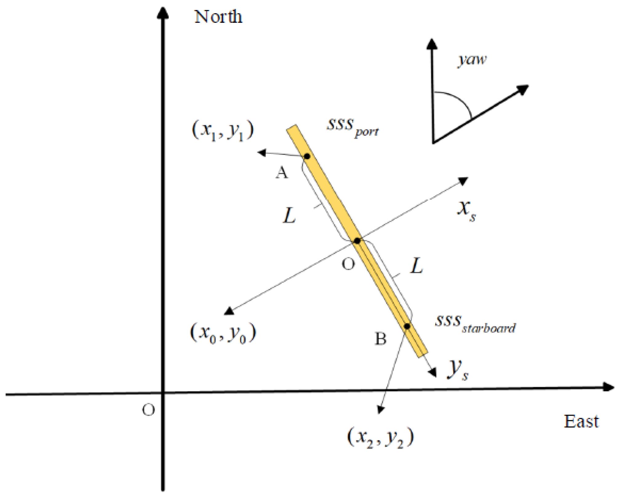
Figure 6 The relationship between sonar data frame data and global positioning.

According to the above analysis, the conversion formula from the coordinates of sonar pixels $(x_{s0},y_{s0})$ in the carrier coordinate system to the global coordinate system $(x,y)$ can be obtained as shown in below. In order to ensure consistency in matrix calculation, two-dimensional coordinates are extended to three-dimensional coordinates.

$$\left[\begin{array}{c}x\\ y\\ 1\end{array}\right]=R_1{R}_2\left[\begin{array}{c}{x}_{s0}\\ y_{s0}\\ 1\end{array}\right]=\left[\begin{array}{ccc}1& 0& x_0\\ 0& 1& y_0\\ 0& 0& 1\end{array}\right]\left[\begin{array}{ccc}\cos (-yaw)& -\sin (-yaw)& 0\\ \sin (-yaw)& \cos (-yaw)& 0\\ 0& 0& 1\end{array}\right]\left[\begin{array}{c}{x}_{s0}\\ y_{s0}\\ 1\end{array}\right]$$

According to Figure 6, for data points A and B on the port and starboard sides, the global positioning of the known transducer coordinate point O is $(x_0,y_0)$, and based on the calculated horizontal distance Hd, where $L=Hd$, the carrier coordinate system coordinates of data points A and B can be obtained, as shown below.

$$\{\begin{array}{l}A:x_{s0}=-L,y_{s0}=0\\ B:x_{s0}=L,y_{s0}=0\end{array}$$

In addition, the default origin of computer images is the upper left corner, the right is the positive x-axis direction, and the down is the positive y-axis direction. Therefore, in order to ensure that the image can be located in the global coordinate system of the middle and northeast of the image as much as possible, corresponding coordinate transformations are still needed.

Before actual image stitching, it is necessary to convert the coordinate units mentioned above from meters to pixels. According to the image resolution of 1.4 cm*1.4 cm introduced earlier, $R_r=0.014 m$. The complete coordinate transformation of pixels on the sonar data frame from the carrier coordinate system to the image coordinate system can be obtained, as shown below:

$$\left[\begin{array}{c}{x}^{\prime }\\ y^{\prime }\\ 1\end{array}\right]=\frac{1}{0.014}{R}_3{R}_4{R}_1{R}_2\left[\begin{array}{c}{x}_{s0}\\ y_{s0}\\ 0.014\end{array}\right]$$

4.2 Overlap and gap handling

After assigning global positioning to the sonar data frames, due to the discretization of positioning and the presence of heading angles, the seamless continuity between consecutive sonar data frames is disrupted, resulting in considerable gaps or overlaps between frames. Therefore, to maintain the integrity and visibility of the images, it becomes necessary to fill these gaps and blend the overlapping regions. The relationship between the sonar data frames with localization and the sonar data frames with the route is illustrated in Figure 2C. Additionally, owing to the placement of side-scan sonar on both sides of the AUV, the distribution of sonar data frames is perpendicular to the tangent of the route.

To address the overlap issue during the stitching process of sonar data frames, the Root Mean Square (RMS) method can be employed. This method aims to fully utilize the data from each sonar data frame and effectively highlight prominent features. The computational formula is presented as follows.

$$f(i,j)=\frac{1}{n}\sqrt{{\displaystyle \sum _{k=1}^n{f}_k^2(i,j)}}$$

where $f(i, j)$ represents the final pixel intensity at coordinates $(i, j)$, and $f_k(i, j)$ represents the pixel intensity at coordinates $(i, j)$ for the k-th sonar data frame.

To address the issue of gaps during the stitching process, the commonly used region filling algorithm in computer graphics, namely the scan-line filling method, can ensure seamless filling of the target area. This method operates in two directions: along the x-axis and along the y-axis, yet their fundamental principles remain the same. By observing the relative positions of sonar data frames, it is apparent that the areas requiring filling form convex quadrilateral regions bordered by two sonar data frames (where any path connecting any two points within the region remains inside it). Hence, employing the scan-line filling method, assuming extension along the x-axis, the basic procedure of the algorithm can be summarized as follows:

a. Determine the minimum and maximum x-coordinates of the area to be filled, denoted as x₁ and x₂, respectively.

b. Iterate through each scan line $x=a,a\in [x_1,x_2]\&a\in Z$.

c. Compute the intersection points between the scan line and the boundaries of the target area at $x=a$, and record the maximum and minimum values as $y_{a1}$ and $y_{a2}$, respectively.

d. Iterate through each pixel along $y_a=b,a\in [y_{a1},y_{a2}]\&b\in Z$. Calculate the pixel intensity at coordinate $(a, y_a)$ and fill the pixel.

e. Repeat steps 2 to 4 until all pixels within the region are filled.

Throughout this process, the computation of pixel intensity in step d utilizes the inverse distance weighting method. Its expression is presented as follows.

$$I=(\frac{1}{s_1}{I}_{A_1}+\frac{1}{s_2}{I}_{A_2}+\frac{1}{s_3}{I}_{A3}+\frac{1}{s_4}{I}_{A_4})/{\displaystyle \sum _{i=1}^4\frac{1}{s_i}}$$

where I represents the intensity of the pixels to be filled, $I_A$ and s represent the intensity of the four corner points in the region and the Euclidean distance from the pixel to be filled. The specific schematic diagram is shown in Figure 7.

Figure 7

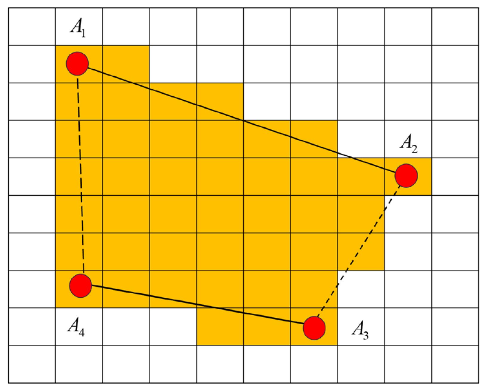
Figure 7 Scanning filling method filling schematic diagram.

It can be observed that the scan-line filling method effectively handles all pixels between two-line segments. By employing the inverse distance weighting method, the pixel intensity at the filling point is predominantly influenced by the intensity of the nearest corner pixel, while being minimally affected by the farthest corner pixel intensity, aligning with realistic expectations. Furthermore, this approach ensures a uniform variation of pixel intensity within the filling area, thus mitigating abrupt changes in pixel intensity.

In practical application, the four corner points are selected from the actual data collected by four adjacent side-scan sonars.

4.3 Overall process of side scan sonar image stitching

In an AUV system, the navigation and side-scan sonar are two distinct modules. Therefore, achieving the stitching of side-scan sonar images requires addressing the matching problem between positioning data and sonar data. In the navigation system, the update frequency of positioning is determined by the sensor frequency, and the update frequency of the DVL (Doppler Velocity Log) generally exceeds that of GPS. However, since positioning data is calculated by a fusion positioning algorithm (Lin et al., 2023), the positioning frequency can be aligned with the DVL sensor frequency, set as $f_D$. The data update frequency of the side-scan sonar is determined by the maximum slant range and the speed of sound in water, which can be expressed as follows:

$$f_s=\frac{v_s}{2·R_{\max }}$$

where $f_s$ is the data update frequency of the side scan sonar, $R_{max}$ is the maximum oblique range set by the side scan sonar, and $v_s$ is the propagation speed of sound waves in water.

In practical applications, the positioning frequency $f_D$ of the DVL is set at 10 Hz. Utilizing the HaiZhuo TongChuang ES1000 side-scan sonar with a maximum slant range $R_{max}=75 m$ and a sound speed $v_s\approx 1500 m/s$, we can calculate the update frequency $f$ of the side-scan sonar data to also be 10 Hz. Hence, maintaining a nearly identical update frequency between the positioning system and the side-scan sonar data is feasible. Consequently, simultaneous recording of the latest positioning data alongside side-scan sonar data allows for one-to-one correspondence between positioning and sonar data, effectively resolving the matching issue.

The complete procedure for side-scan sonar image stitching is outlined as follows:

a. At the onset of stitching, feed both positioning data and side-scan sonar data into the program.

b. Apply preprocessing methods outlined in Section 3 to process the raw sonar data.

c. Employ the sensors carried by the AUV along with their positioning algorithms to obtain corresponding positioning for the sonar data frames.

d. Utilize the geographical encoding method described in Section 4.1 to encode the sonar data.

e. Address gaps and overlaps generated from processing geographical encoding as discussed in Section 4.2.

f. Iterate steps d and e until all side-scan sonar data frames are stitched together.

5 Autonomous perception of targets

Utilizing side-scan sonar for monitoring the sedimentation of underwater targets within a designated area is one of the objectives of ocean pasture environmental surveillance. Hence, to enable AUVs equipped with side-scan sonars to autonomously perceive underwater targets, a method based on a classification algorithm for autonomous target perception has been proposed. The aforementioned approach extracts pertinent information from real-time data captured by the side-scan sonar to generate effective area images. Upon obtaining these images, this chapter first employs the EfficientNet classification algorithm to discern the presence or absence of targets within the effective area images. Images containing targets undergo comprehensive processing, including non-local means filtering, K-means clustering, and an improved region-scalable fitting model for segmentation. This process facilitates the automatic segmentation of target shadow regions within side-scan sonar images, with the effectiveness of the method validated through experimentation. Finally, target height monitoring is achieved using shadow-based height estimation. The specific procedure is illustrated in Figure 2D.

5.1 Target existence judgment based on classification algorithms

In the operation of side-scan sonar systems, there are dark zones between the seabed line and the transmission line. Additionally, during practical use, there may be ineffective areas at the tail end due to mismatches between the set range and the actual maximum slant range. The region lying between the dark zones and the ineffective tail end constitutes the effective area. Figure 8 illustrates the geometric relationship of the side-scan sonar system.

Figure 8

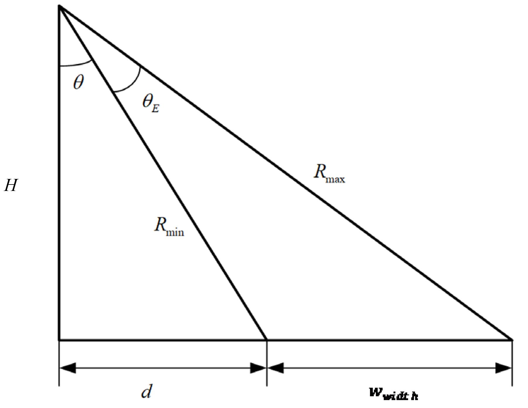
Figure 8 Geometric relationship diagram of side scan sonar system.

θ is the tilt angle when installing the side scan sonar. When vertically downward θ = 0, θ_E is the vertical beam width of the side scan sonar, H is the height of the transducer from the bottom, R_min and R_max are the minimum and maximum slant distances in the effective area, d is the horizontal distance between the seabed point and the transducer caused by oblique installation, and w_width is the horizontal width in the effective area.

Based on the geometric relationship of the side scan sonar system, the position of the effective region in the side scan sonar image is derived, namely the values of R_min and R_max. Assuming that the result of seabed detection is s, measured in pixels, R_min can be expressed as follows.

$$R_{\min }=s$$

Calculate based on the triangular relationship:

$$H=R_{\min }\cos \theta$$

$$R_{\max }=\frac{H}{\cos (\theta +{\theta }_E)}=\frac{R_{\min }\cos \theta }{\cos (\theta +{\theta }_E)}=\frac{s\cos \theta }{\cos (\theta +{\theta }_E)}$$

Based on the above, the oblique range $(s,\frac{s\cos \theta }{\cos (\theta +{\theta }_E)})$ of the effective area can be obtained, where s is the position of the detected seabed line.

Under normal circumstances, install the tilt angle θ If it is very small or 0, then $R_{max}$ can be further simplified as follows, and the diagonal interval of the effective region can be represented as $(s,\frac{s}{\cos {\theta }_E})$.

$$R_{\max }=\frac{s\cos (0)}{\cos (0+{\theta }_E)}=\frac{s}{\cos {\theta }_E}$$

To implement the EfficientNet image classification algorithm for determining the presence or absence of targets in images, we conducted experiments using side-scan sonar data. To evaluate the effectiveness of EfficientNet on side-scan sonar data, we created a dataset by extracting relevant regions from original side-scan sonar images, comprising two classes: images with targets and images without targets. The model was trained on this dataset and subsequently tested using publicly available datasets.

In preparing the dataset, we employed seabed line detection methods to extract the regions of interest from the images and fixed the height of each image at 200 pixels to form the image dataset for classification training. Unlike specific object classification, our task involved categorizing images broadly into two classes: “haveTarget” and “noTarget”. Target presence or absence was determined by matching highlighted areas and shadow regions within the images. Additionally, during training, 10% of the dataset was reserved for validation. Examples of images with and without targets illustrated in Figure 9.

Figure 9

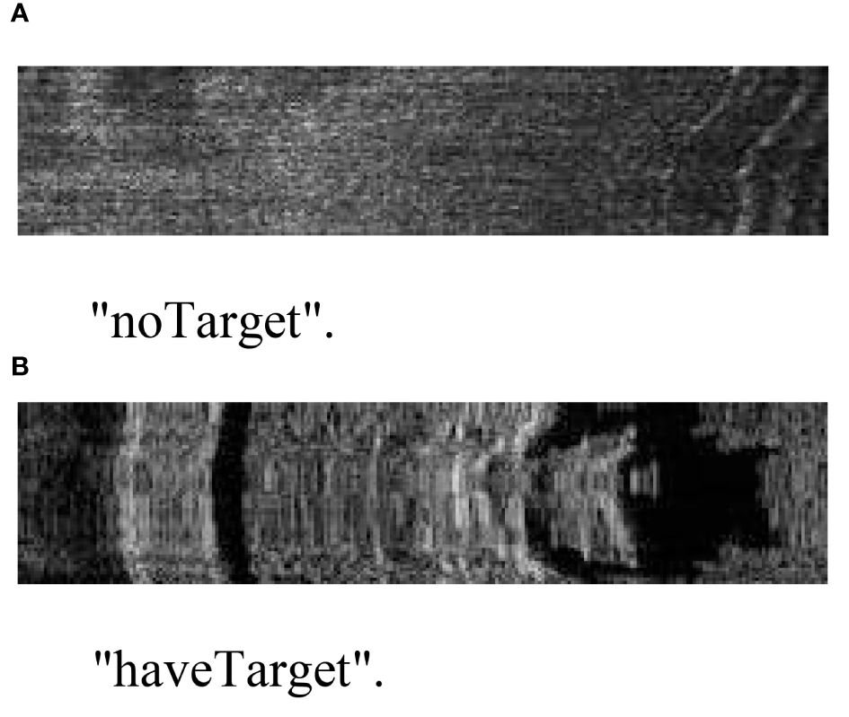
Figure 9 Example of dataset with or without target images. (A) “noTarget”. (B) “haveTarget”.

The dataset is split into training and validation sets, with a data ratio of 9:1 between the training and validation sets. Figure 10 shows the variation process of the loss function value during model training. It can be observed that both the training set loss value and the validation set loss value can quickly converge to a lower level and remain stable during the training process.

Figure 10

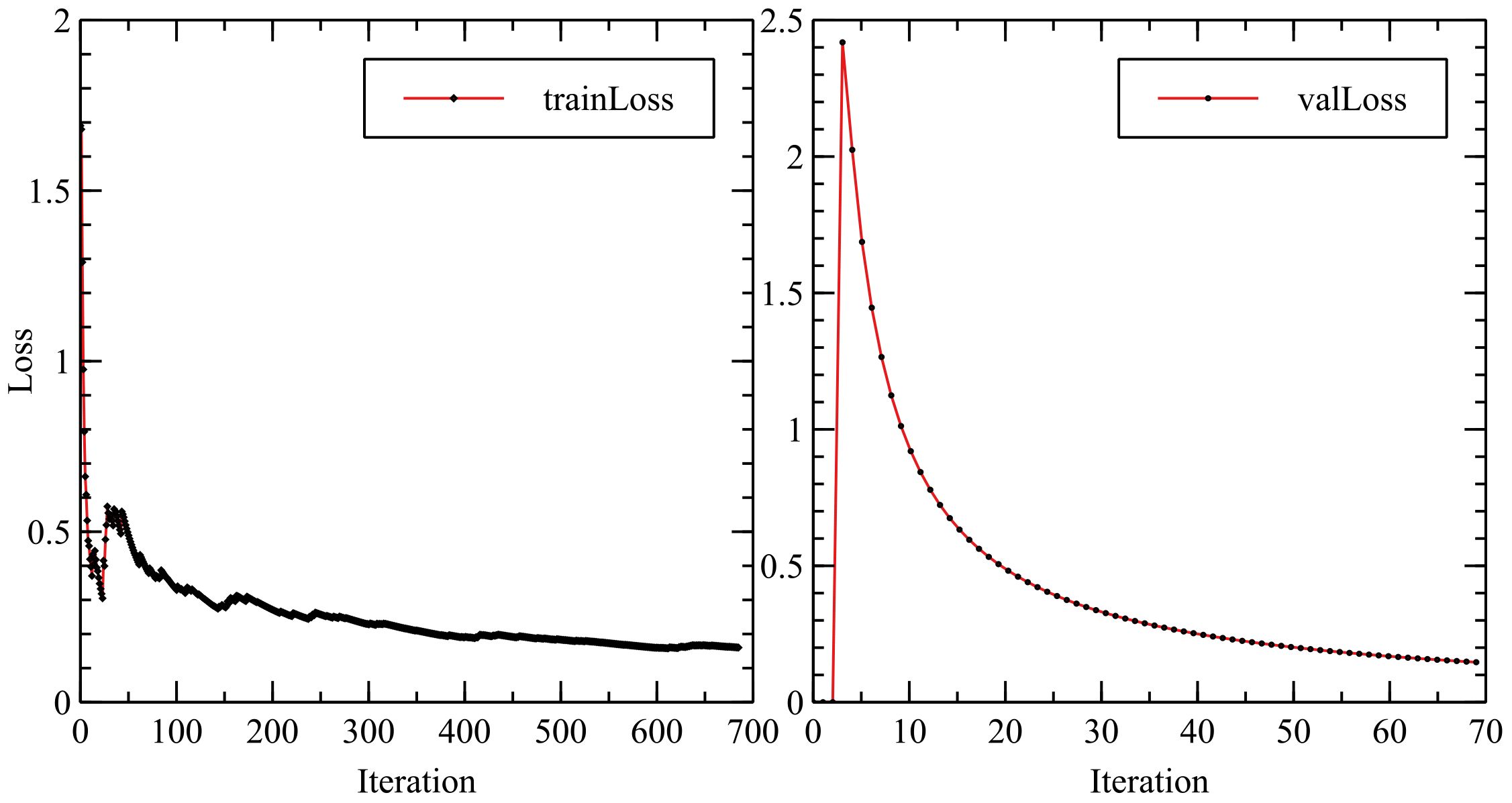
Figure 10 Changes in loss values during training.

After obtaining the trained model, we conducted tests to evaluate its classification performance on a Lenovo Yoga 14sITL 2021 laptop equipped with an Intel Core i5–1135G7 processor. To assess the generalization capability of the method, we employed the publicly available dataset from Hohai University consisting of side-scan sonar images of underwater aircraft wreckage and shipwrecks for model classification testing. This dataset comprises a total of 447 images, including 385 shipwreck images and 62 aircraft wreckage images, all of which contain targets. The specific model testing results are presented in Table 3.

Table 3

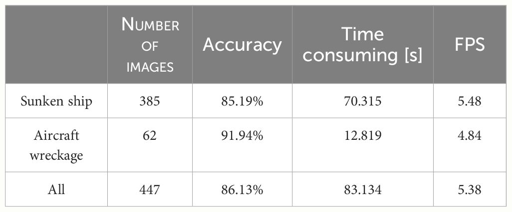
Table 3 The model testing results.

Figure 11 provides examples of classification results, where the “class” field indicates the classification result generated by the model (“haveTarget” denotes the presence of a target in the image, while “noTarget” indicates its absence), and the “time” field represents the time taken to classify the current image.

Figure 11

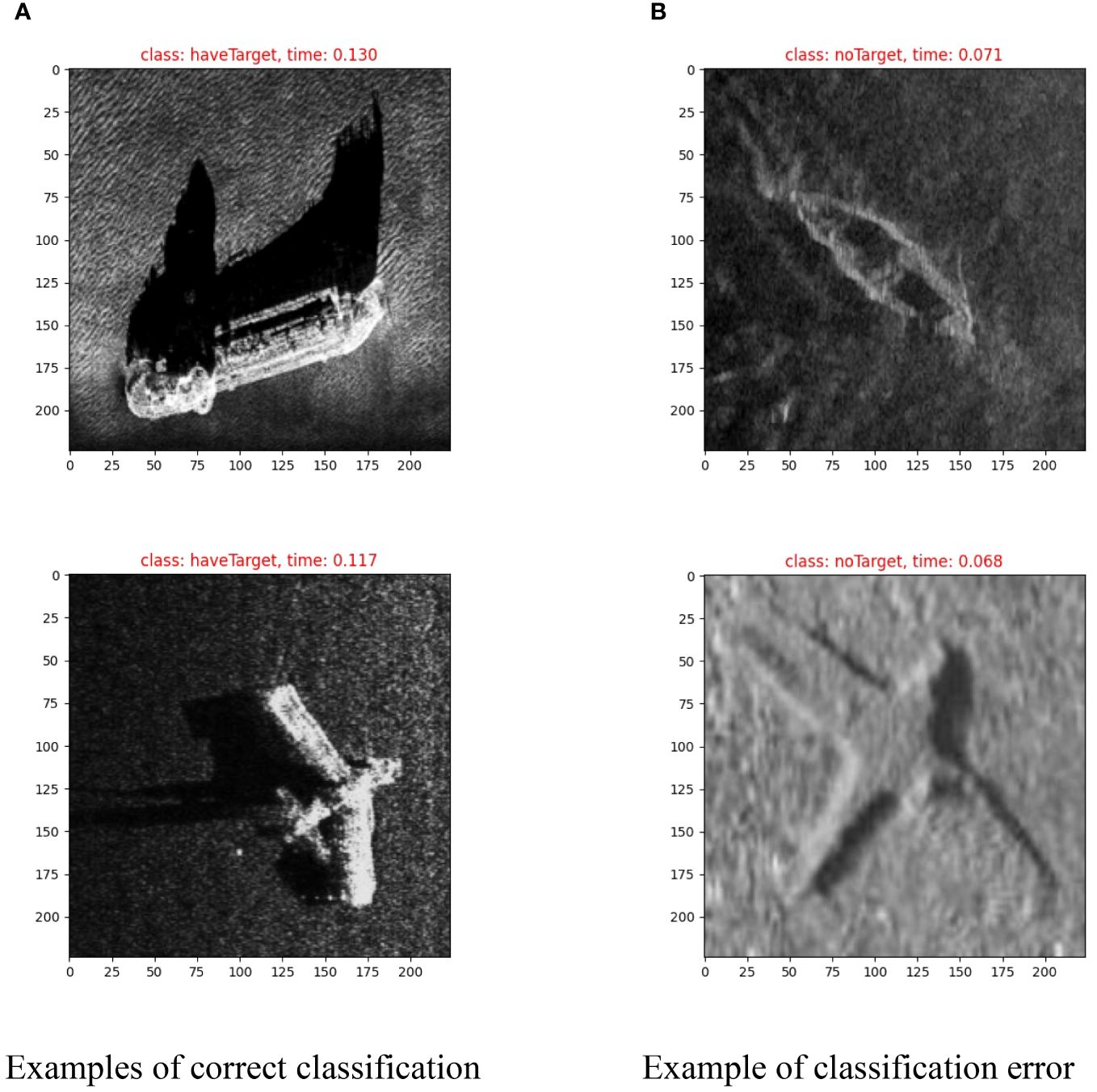
Figure 11 Example of test results. (A) Examples of correct classification. (B) Example of classification error.

Upon examination of the results, the overall accuracy of the classification is approximately 86%, indicating a relatively high level of accuracy. Instances of misclassification primarily occur in images lacking the basic features of highlighted and shadowed areas, as depicted in Figure 11B, partly due to disparities between the training and testing datasets.

Furthermore, an observation of the table reveals that the image classification speed is fast, reaching around 5.36 frames per second. Considering that the acquisition time for a single frame of side-scan sonar data is approximately 0.1 seconds, the classification algorithm can effectively process images at the rate of one per frame, meeting the requirements for real-time processing.

5.2 Target height estimation

Underwater sonar images exhibit characteristics such as uneven intensity and high noise levels, which can significantly impede observation of underwater targets and the effectiveness of automated segmentation. In order to achieve precise segmentation of the shadow regions within side-scan sonar images, a segmentation method is employed that combines non-local means (NLM) filtering, K-means clustering, and Region-Scalable Fitting (RSF) energy minimization. Through testing, suitable filtering parameters are selected, and the accuracy of clustering is enhanced by optimizing the number of K-means cluster centers. Additionally, the energy function of the RSF model is adjusted according to practical considerations to better align with the realities of shadow segmentation.

The specific process of target segmentation can be found in Appendix. After obtaining the target, the target height is estimated using the following method.

According to the detection principle of side scan sonar, the oblique range is distinguished based on the time of sound wave return. When a target object with a certain height appears, there will be no sound wave signal return in the oblique range behind the target object, which will cause certain shadows on the image. Based on this principle, the height of the target object can be inferred by using the length of the shadow caused by the target object (Bikonis et al., 2013). Based on the detection principle of side scan sonar, the geometric relationship diagram of the target object can be obtained as shown in Figure 12.

Figure 12

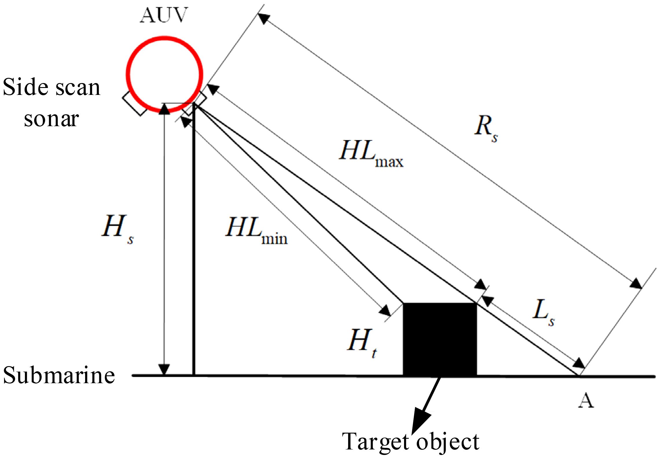
Figure 12 Geometric relationship diagram of the target object.

$H_s$ is the height of the side scan sonar from the bottom, $H_t$ is the height of the target object, $H{L}_{\min }$ and $H{L}_{\max }$ are the minimum and maximum slant distances of the bright area caused by the target object, $R_s$ is the farthest slant distance of the shadow, and $L_s$ is the length of the slant distance of the shadow caused by the target object. Based on geometric relationships, the height of the target object can be intuitively inferred as follows:

$$H_t=\frac{L_s}{R_s}·H_s$$

where $H_s$ can be obtained based on the seabed detection results. $H{L}_{\max }$ and $R_s$ can be segmented based on the aforementioned images. Assuming that the distance from the seabed to the radiation is $s_i$ pixels, and the horizontal resolution of the side scan sonar original image is $R_r$., it can be converted as follows.

$$H_t=\frac{Rs-H{L}_{\max }}{R_s}{s}_{i}Rr$$

To verify the effectiveness of the height estimation method mentioned above, experimental verification was conducted in a water tank. The specific experimental scenario is shown in Figure 13.

Figure 13

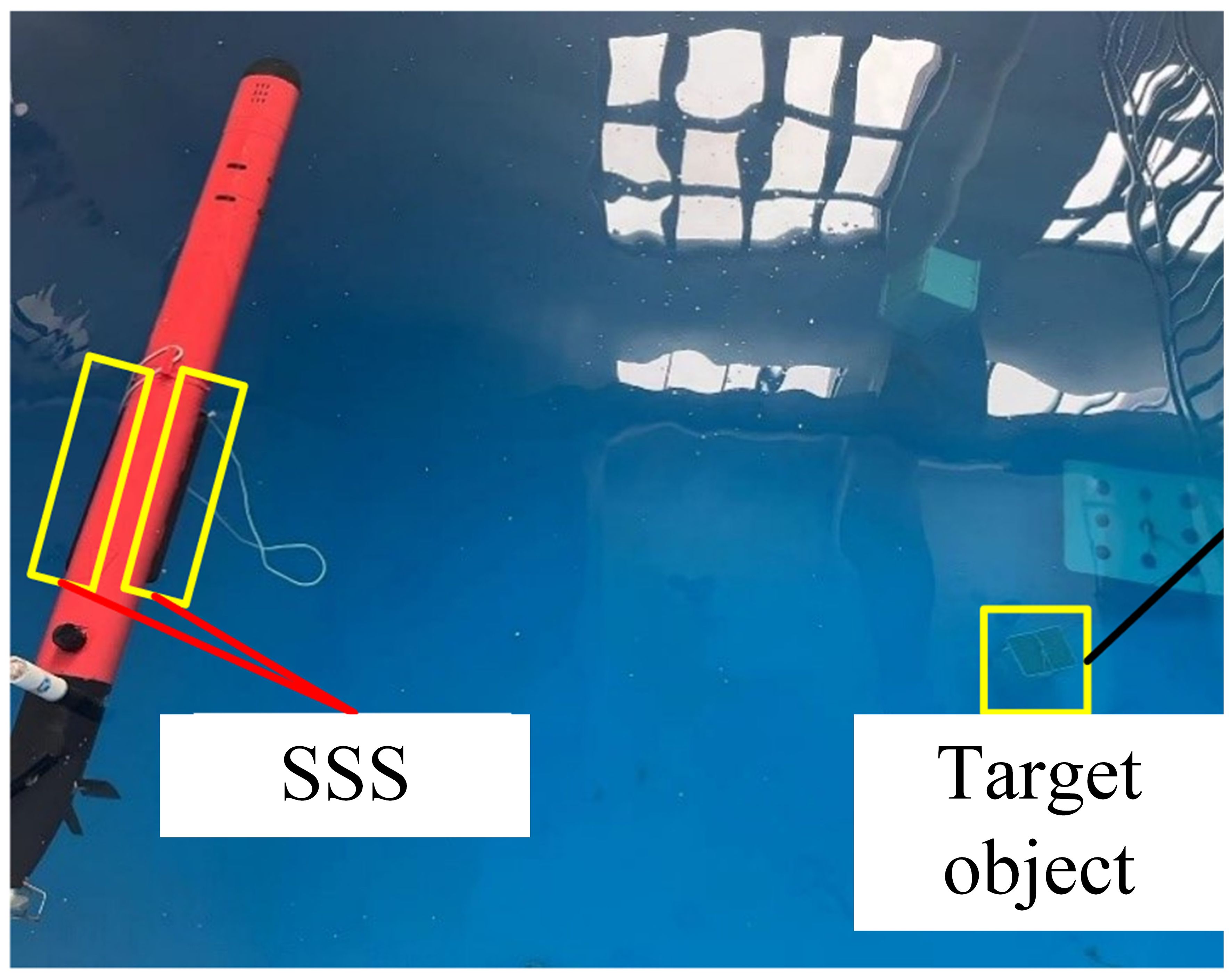
Figure 13 Target height calculation test in the pool.

The actual measurement value of the height of the object is 60 cm. The relevant side scan sonar data was obtained by scanning with a side scan sonar, and the collected data is shown in Figure 14.

Figure 14

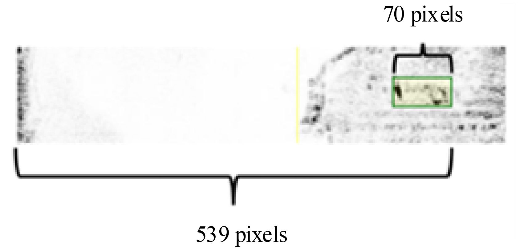
Figure 14 Sonar image of the measured object.

The depth of the water tank is 5.05 m. According to the height calculation formula calculated above, the calculation result is shown as follows.

$$H_t=\frac{Rs-H{L}_{\max }}{R_s}{s}_i{R}_r=\frac{70}{539}\times 505\text{cm}=65.6\text{cm}$$

Based on the actual height of the object of 60 cm, an error rate of 9% can be calculated. Therefore, this height calculation method can to some extent reflect the actual height of the object.

5.3 Overall process of target autonomous perception

This section presents an autonomous perception framework for target detection in side-scan sonar images based on the EfficientNet classification algorithm, aimed at monitoring targets during AUV cruises in marine farms, as illustrated in Figure 15. To address the challenge of complex target perception caused by the original side-scan sonar images, a method is proposed to extract effective regions from the images based on seabed line detection results. Subsequently, the EfficientNet classification algorithm is utilized to determine the presence or absence of targets in these regions, reducing the burden of shadow segmentation and validated through experiments. To enhance the accuracy of shadow segmentation, a combination of NLM filtering, K-means clustering, and RSF is employed. Target height is calculated using a shadow-based height estimation method and tested through pool experiments.

Figure 15

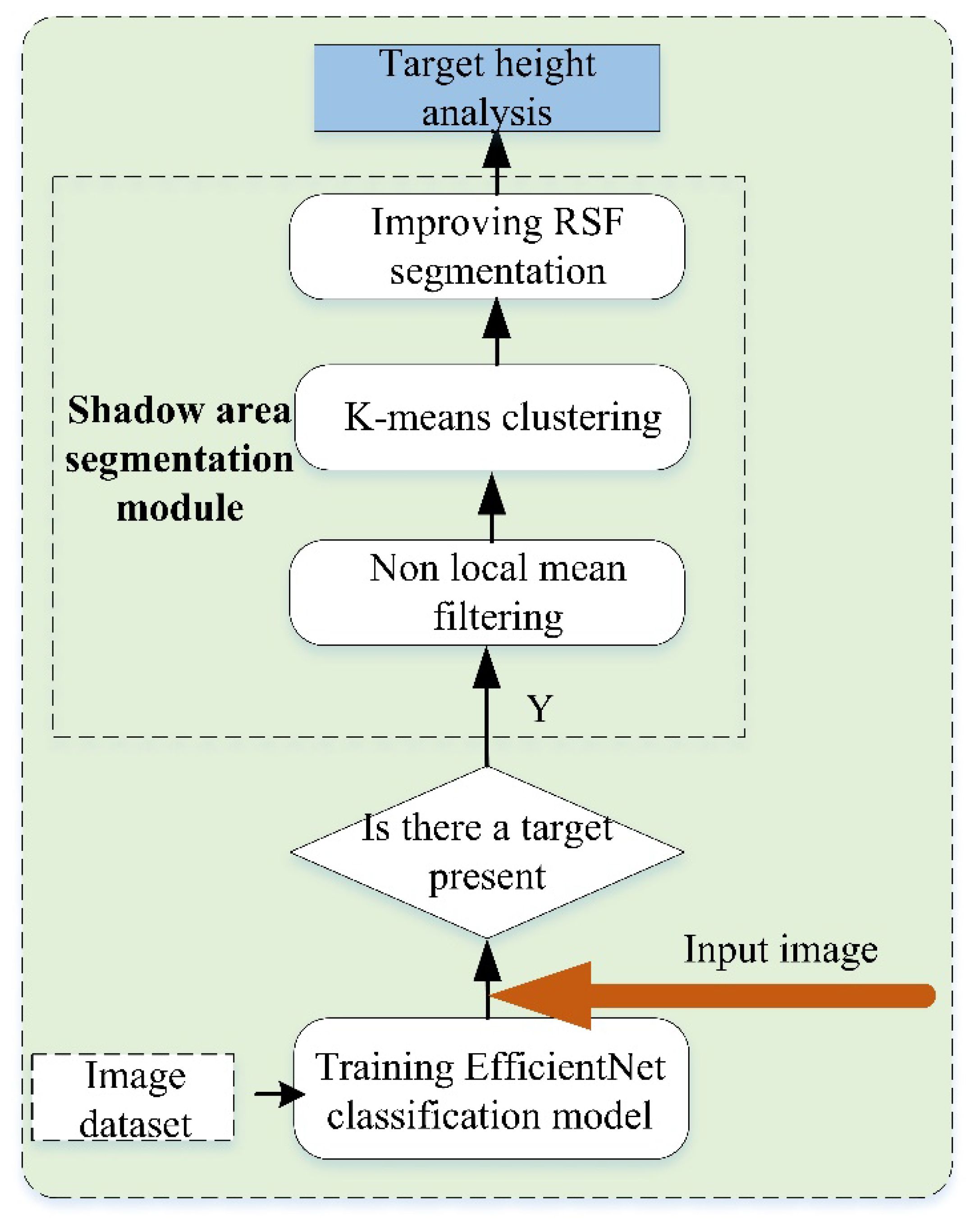
Figure 15 The entire process of target recognition.

6 Results

To achieve autonomous data collection with side-scan sonar, the AUV platform needs to be utilized, enabling it to autonomously navigate both on the water surface and underwater to meet the requirements of autonomous monitoring. The vehicle utilized in this study is a torpedo-shaped AUV (Zhang et al., 2022), as depicted in Figure 16. The side-scan sonar utilized is the ES1000 from Hai Zhuo Tong Chuang, operating at a frequency of 900 kHz, with a maximum slant range of 75 m, a horizontal beam width of 0.2°, a vertical beam width of 50°, and a vertical heading resolution of 1 cm. It is embedded on the side of the AUV. To validate the proposed algorithms, the side-scan sonar is mounted, and experiments are conducted in the Qingjiang area of Hubei, China.

Figure 16

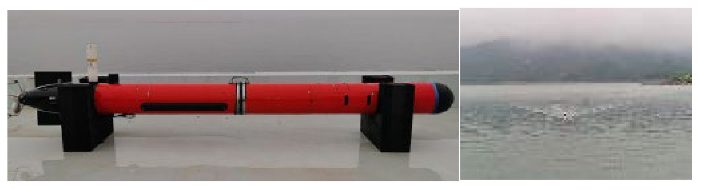
Figure 16 AUV and AUV working in Qingjiang.

6.1 Autonomous acquisition and stitching experiment of side scan sonar images

Prior to utilizing the positioning data from the AUV, frame-to-frame data is tightly stitched together to obtain waterfall plots of the raw sonar data, which are then color-rendered, resulting in Figure 17A. Using the proposed seabed line detection method, the side-scan sonar images are analyzed for seabed line detection, with specific results shown in Figure 17B. Due to the unpredictable nature of the field environment, it is not possible to accurately measure the true underwater depth for every frame. However, in Figure 17B, it is evident that the seabed line detection closely aligns with the boundary between light and dark regions. Moreover, analyzing the seabed line detection results from the left and right-side sonar images reveals consistent results in the majority of intervals, indicating that due to the close spacing between the left and right-side sonars, their respective heights above the seabed should theoretically be consistent, which is confirmed by the actual detection results, thus validating the accuracy of seabed line detection. Following the seabed line detection, the images undergo corresponding radiometric and slant range corrections, with interpolation applied to fill gaps resulting from slant range correction to ensure smooth transitions in pixel intensities. The corrected images are depicted in Figure 17C. The transition from slant range-based positioning to horizontal distance-based positioning is seamless, further validating theoretical effectiveness. Additionally, due to varying seabed line heights in each sonar data frame, the effective width of each frame also differs, which is reflected in the subsequent image stitching process. Through the aforementioned processes, processed valid data is obtained from the raw sonar data. Subsequently, the obtained positioning data is combined with the sonar data to generate final stitched images reflecting global geographical locations. The actual stitching results, as shown in Figure 17D, demonstrate the terrain surrounding the actual trajectory with minimal gaps and smooth image transitions, aligning with theoretical analysis. Moreover, given the variation in seabed lines, the amount of valid data differs across different sonar data frames, thus validating the effectiveness of AUV autonomous data collection and image stitching theory.

Figure 17

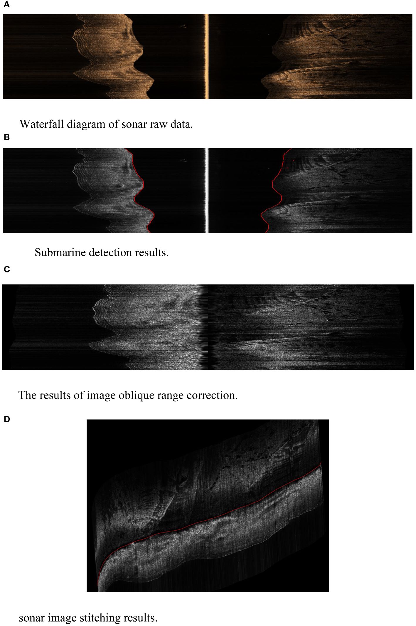
Figure 17 Autonomous acquisition and stitching experiment of side scan sonar images. (A) Waterfall diagram of sonar raw data. (B) Submarine detection results. (C) The results of image oblique range correction. (D) sonar image stitching results.

6.2 Target autonomy perception experiment

Controlled by the upper computer within the AUV, autonomous navigation is achieved while perceiving underwater targets and segmenting target shadow regions during navigation.

To extract valid regions from raw side-scan sonar images, the seabed line detection is initially performed on the raw images. The result of seabed line detection for a single image is illustrated in Figure 18A, where the red dots represent the detection results. Figure 18B presents the valid region image after eliminating invalid areas. These obtained local images of valid regions are then fed into a classification program to determine the presence of targets. Figure 18C displays the classification algorithm’s determination of target existence, with “class” indicating “haveTarget” when a target is detected, and “time” denoting the time taken for image classification. Following the designed workflow, images identified as containing targets proceed to the target shadow region segmentation program, where accurate segmentation of the shadow regions is conducted, and the relevant results are preserved. Figure 18C showcases the segmentation results of shadow regions in the aforementioned images. It’s observed that this process effectively separates the shadow regions from the images. After obtaining the segmented images of shadow regions, height calculation for targets is conducted based on height estimation principles, yielding the height of the targets. Figure 18D represents the results of height analysis.

Figure 18

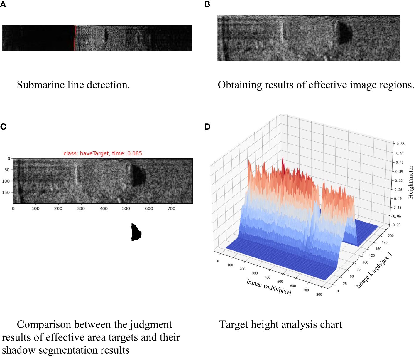
Figure 18 Target autonomy perception experiment. (A) Waterfall diagram of sonar raw data. (B) Submarine detection results. (C) The results of image oblique range correction. (D) sonar image stitching results.

Thus, the entire process of collecting target shadow regions from side-scan sonar images has been successfully validated, affirming the effectiveness of this target perception framework.

7 Conclusions

The paper initially delves into the issue of seabed line detection in side-scan sonar images, considering the characteristics of such images. To address existing problems in detection methods, such as weak robustness or complex processes, a seabed line comprehensive detection method based on the sliding window approach is proposed. This method offers strong robustness and relatively simple processes. Validation is carried out through pool and lake experiments. The experimental results demonstrate a 31.2% increase in accuracy for our proposed method compared to the final peak method. Integration of seabed line detection, radiometric correction, and slant range correction completes the preprocessing of side-scan sonar images.

The maneuverability of the AUV results in varying heading angles and positions for each sonar image frame, posing challenges for stitching the sonar images between frames. While existing literature focuses on stitching distinct sonar images, we approached the task by addressing the gaps and overlaps between consecutive frames for seamless image stitching. Addressing the challenge of matching sonar data with positioning data in image stitching, the transformation relationship between the AUV carrier coordinate system and the global North-East-Down coordinate system is derived. Formulas for pixel coordinate transformation are provided. Subsequent treatment is applied to address gaps and overlaps in geographic coding, enabling autonomous collection and stitching of underwater terrain data.

We propose a lightweight, high-frequency target automatic recognition framework. This framework not only identifies targets but also computes their heights. EfficientNet is adopted as the determination network for target existence in sonar images. Training and validation datasets are constructed accordingly to obtain a classification model through training. Target recognition runs an average of over 5 images per second. Methods for target shadow segmentation are explored. Within the framework of filtering, coarse segmentation, and fine segmentation, an approach is proposed to enhance the accuracy of coarse segmentation by increasing the number of K-means clustering centers. This provides more precise initial contours for subsequent fine segmentation, thereby reducing the number of iterations required. After target segmentation, shadow information is used to calculate the height of the target. In the validation experiments conducted in the pool, the height measurement error was found to be 9%. Finally, the effectiveness of the method is verified through lake experiments.

In future work, under the scenario of AUV navigation along predetermined routes, target recognition can be achieved through target perception if the target positions are known. This aspect can subsequently serve as auxiliary positioning for AUVs.

Data availability statement

The original contributions presented in the study are included in the article/supplementary material. Further inquiries can be directed to the corresponding authors.

Author contributions

ZZ: Writing – review & editing, Project administration, Methodology, Conceptualization. RW: Writing – original draft, Methodology, Conceptualization. DL: Writing – review & editing. ML: Writing – review & editing, Funding acquisition, Formal analysis. SX: Writing – review & editing, Funding acquisition. RL: Writing – review & editing, Validation.

Funding

The author(s) declare financial support was received for the research, authorship, and/or publication of this article. This research was financially support by the Science and Technology Innovation 2025 Major Special Project of the Ningbo Major Science and Technology Task Research Project (2022Z058), the Natural Science Foundation of China (52101404), the Natural Science Foundation of Zhejiang Province (LY23E090002), and the China Postdoctoral Science Foundation (2023M733072).

Conflict of interest

The authors declare that the research was conducted in the absence of any commercial or financial relationships that could be construed as a potential conflict of interest.

Publisher’s note

All claims expressed in this article are solely those of the authors and do not necessarily represent those of their affiliated organizations, or those of the publisher, the editors and the reviewers. Any product that may be evaluated in this article, or claim that may be made by its manufacturer, is not guaranteed or endorsed by the publisher.

References

Abu A., Diamant R. (2019). Enhanced fuzzy-based local information algorithm for sonar image segmentation. IEEE Trans. Image Process. 29, 445–460. doi: 10.1109/TIP.2019.2930148

CrossRef Full Text | Google Scholar

Bay H., Tuytelaars T., Van Gool L. (2006). SURF: Speeded Up Robust Features. In: Leonardis A., Bischof H., Pinz A. editors. Computer Vision – ECCV 2006. Meeting9th European Conference on Computer Vision (ECCV 2006). Lecture Notes in Computer Science, vol 3951; 2006 May 07-13; Graz, Austria. doi: 10.1007/11744023_32

CrossRef Full Text | Google Scholar

Bikonis K., Moszynski M., Lubniewski Z. (2013). Application of shape from shading technique for side scan sonar images. Polish Maritime Res. 20, 39–44. doi: 10.2478/pomr-2013-0033

CrossRef Full Text | Google Scholar

Chenyang P., Jerry L. (1998). Snakes, shapes, and gradient vector flow. IEEE Trans. Image Processing. 7 (3), 359–369. doi: 10.1109/83.661186

CrossRef Full Text | Google Scholar

Huo G., Yang S. X., Li Q., Zhou Y. (2016). A robust and fast method for sidescan sonar image segmentation using nonlocal despeckling and active contour model. IEEE Trans. Cybernetics 47, 1–18. doi: 10.1109/TCYB.2016.2530786

CrossRef Full Text | Google Scholar

Hurtós N., Ribas D., Cufí X., Petillot Y., Salvi J. (2015). Fourier-based registration for robust forward-looking sonar mosaicing in low-visibility underwater environments. J. Field Robotics 32, 123–151. doi: 10.1002/rob.21516

CrossRef Full Text | Google Scholar

Jianhu Z., Xiaodong S., Hongmei Z. (2018). Side-scan sonar image mosaic using couple feature points with constraint of track line positions. Remote Sens. 10, 953. doi: 10.3390/rs10060953

CrossRef Full Text | Google Scholar

Kim B., Joe H., Yu S. C. (2021). High-precision underwater 3D mapping using imaging sonar for navigation of autonomous underwater vehicle. Int. J. Control Automation Syst. 19 (9), 3199–3208. doi: 10.1007/s12555-020-0581-8

CrossRef Full Text | Google Scholar

Li C., Kao C. Y., Gore J. C., Ding Z. (2008). Minimization of region-scalable fitting energy for image segmentation. IEEE Trans. Image Process. 17, 1940–1949. doi: 10.1109/TIP.2008.2002304

PubMed Abstract | CrossRef Full Text | Google Scholar

Lin M., Lin R., Li D., Yang C. (2023). Light beacon-aided AUV electromagnetic localization for landing on a planar docking station. IEEE J. Oceanic Eng. 48, 677–688. doi: 10.1109/JOE.2023.3265767

CrossRef Full Text | Google Scholar

Lin M., Lin R., Yang C., Li D., Zhang Z., Zhao Y., et al. (2022). Docking to an underwater suspended charging station: Systematic design and experimental tests. Ocean Eng. 249, 110766. doi: 10.1016/j.oceaneng.2022.110766

CrossRef Full Text | Google Scholar

Lin M., Yang C. (2020). Ocean observation technologies: A review. Chin. J. Mechanical Eng. 33, 1–18. doi: 10.1186/s10033-020-00449-z

CrossRef Full Text | Google Scholar

Lowe D. (2003). Distinctive image features from scale-invariant key points. Int. J. Comput. Vision 20, 91–110. doi: 10.1023/B:VISI.0000029664.99615.94

CrossRef Full Text | Google Scholar

Mignotte M., Collet C., Pérez P., Bouthemy P. (1999). Three-class Markovian segmentation of high-resolution sonar images. Comput. Vision Image Understanding 76, 191–204. doi: 10.1006/cviu.1999.0804

CrossRef Full Text | Google Scholar

Pal N. R., Pal K., Keller J. M., Bezdek J. C. (2005). A possibilistic fuzzy c-means clustering algorithm. IEEE Trans. Fuzzy Syst. 13, 517–530. doi: 10.1109/TFUZZ.2004.840099

CrossRef Full Text | Google Scholar

Qin X., Luo X., Wu Z., Shang J., Zhao D. (2022). Deep learning-based high accuracy bottom tracking on 1-D side-scan sonar data. IEEE Geosci. Remote Sens. Lett. 19, 1–5. doi: 10.1109/LGRS.2021.3076231

CrossRef Full Text | Google Scholar

Ramirez T. M. (2014). Triton Perspective-SS Sidescan Processing Guide. (San Diego, California, USA: Triton Imaging, Inc), 6–7.

Google Scholar

Shang X., Zhao J., Zhang H. (2021). Automatic overlapping area determination and segmentation for multiple side scan sonar images mosaic. IEEE J. Selected Topics Appl. Earth Observations Remote Sens. 14, 2886–2900. doi: 10.1109/JSTARS.2021.3061747

CrossRef Full Text | Google Scholar

Wong J. A. H. A. (1979). Algorithm AS 136: A K-means clustering algorithm. J. R. Stat. Soc. 28, 100–108. doi: 10.2307/2346830

CrossRef Full Text | Google Scholar

Woock P. (2011). “Deep-sea seafloor shape reconstruction from side-scan sonar data for AUV navigation,” in IEEE OCEANS Conference (Santander, Spain: IEEE), 1–7.

Google Scholar

Ye X. F., Zhang R. H., Liu R. X., Guan R. L. (2010). Sonar image segmentation based on GMRF and level-set models. Ocean Eng. 37, 891–901. doi: 10.1016/j.oceaneng.2010.03.003

CrossRef Full Text | Google Scholar

Zhang N., Jin S., Bian G., Chi L. (2021). A mosaic method for side-scan sonar strip images based on curvelet transform and resolution constraints. Sens. (Basel Switzerland). 21, 1–17. doi: 10.3390/s21186044

CrossRef Full Text | Google Scholar

Zhang Z., Lin M., Li D. (2022). A double-loop control framework for AUV trajectory tracking under model parameters uncertainties and time-varying currents. Ocean Eng. 265, 1–15. doi: 10.1016/j.oceaneng.2022.112566

CrossRef Full Text | Google Scholar

Zhang Z., Zhong L., Lin M., Lin R., Li D. (2024). Triangle codes and tracer lights based absolute positioning method for terminal visual docking of autonomous underwater vehicles. Ind. Robot: Int. J. Robotics Res. Application. 51 (2), 269–286. doi: 10.1108/IR-10-2023-0233

CrossRef Full Text | Google Scholar

Zhao J., Wang X., Zhang H., Wang A. (2017). A comprehensive bottom-tracking method for sidescan sonar image influenced by complicated measuring environment. IEEE J. Oceanic Eng. 42, 619–631. doi: 10.1109/JOE.2016.2602642

CrossRef Full Text | Google Scholar

Zheng G., Zhang H., Li Y., Zhao J. (2021). A universal automatic bottom tracking method of side scan sonar data based on semantic segmentation. Remote Sens. 13, 1945. doi: 10.3390/rs13101945

CrossRef Full Text | Google Scholar

Appendix: target shadow segmentation

Non-local means filtering and local filtering share some similarities, both involving calculations based on pixels in the vicinity of a specified pixel. However, there are differences in how the weights of neighboring pixels are calculated. Compared to traditional local filtering, non-local means filtering better preserves edge details.

The computation process of non-local means filtering can be summarized as follows, assuming the coordinates of the specified pixel are (i, j):

a. Selecting the side lengths of the square-shaped similar window F and the search window S, denoted as f and s, respectively.

b. Calculating the initial weights ws of pixels within the similar window F sequentially, according to the following formula:

$$W{(x,y)}_{s\times s}=Kernel(x,y)·{(S(x,y)-S(i,j))}^2$$

$$ws(x,y)=sum(W(x,y))$$

where $W(x,y)$ is the weight matrix at $(x,y)$, $Kernel(x,y)$ is the Gaussian kernel, and $ws(x,y)$ is the corresponding weight value. In addition, matrix multiplication and subtraction in the above formula are corresponding element operations, and $sum(·)$ is the sum of all elements in the matrix.

c. Select the Gaussian smoothing parameter h and use the Gaussian function to smooth the initial weight ws to obtain the final weight w, as shown below.

$$w(x,y)=e^{(- \frac{ws(x,y)}{h^2})}$$

d. Using weights to calculate the weighted average of pixels within similar windows as the filtering result for the specified pixel, as shown below.

$$f^{\prime }(i,j)=\frac{1}{C}{\displaystyle \sum _{x=i-\frac{f-1}{2}}^{i+\frac{f-1}{2}}{\displaystyle \sum _{y=i-\frac{f-1}{2}}^{i+\frac{f-1}{2}}f(x,y)·w(x,y)}}$$

$$C={\displaystyle \sum _{x=i-\frac{f-1}{2}}^{i+\frac{f-1}{2}}{\displaystyle \sum _{y=i-\frac{f-1}{2}}^{i+\frac{f-1}{2}}w(x,y)}}$$

Based on the mathematical principles of non-local means filtering, it can be observed that the parameters f, s, and h significantly influence the filtering effect. Among them, the variation of h has a considerable impact on the filtering effect. A larger Gaussian smoothing parameter, h, implies that the weights of all pixels within the similar window are relatively close, resulting in a tendency towards image blurring and a reduction in intensity differences between pixels. Therefore, it is essential to select an appropriate Gaussian smoothing parameter, h, based on practical considerations when coordinating with segmentation methods.

K-means clustering is an unsupervised data analysis method that can classify data without prior training. Thus, to provide some initial segmentation results for subsequent precise segmentation, K-means clustering is employed to perform coarse segmentation on the sonar images filtered beforehand.

The fundamental principle of K-means clustering is to classify data based on the similarity between data points and cluster centers. The specific process of using K-means for image clustering is as follows:

a. Convert the two-dimensional image into a one-dimensional array.

b. Set a stopping threshold $\epsilon$ or iteration limit “$miterations$“.

c. Randomly initialize n centers, with center values representing the pixel intensity of selected pixels.

d. Define a loss function $J(c,\mu )$, as detailed below:

$$J(c,\mu )={\displaystyle \sum _{i=1}^N{(f(x_i)-f({\mu }_{c_i}))}^2}$$

where N represents the total number of pixels in the image, $f(·)$ represents pixel intensity, and ${\mu }_{c_i}$ represents the center point to which the current pixel belongs.

e. Assign each sample to the center closest to its pixel intensity;

f. For each class k, recalculate the pixel intensity at its center as shown below;

$$f({\mu }_k^{t+1})\le \arg \min {\displaystyle \sum _{x_i\in {\Omega }_k}{(f(x_i)-f(\mu ))}^2}$$

where ${\Omega }_k$ represents all pixels belonging to Class k.

g. Repeat e and g until the loss function $J<\epsilon$ or number of iterations $iteration>miterations$.

In the practical segmentation of shadow areas, the consideration involves distinguishing between shadow and non-shadow regions by clustering the image according to two sets of centroids. However, since the objective is to segment only the shadow regions, enhancing the refinement of shadow segmentation can be achieved by increasing the number of clustering centroids. After obtaining the segmentation results, the class with the lowest average pixel intensity is selected as the shadow region class, while all other classes are designated as non-shadow region classes. With an increase in clustering centroids, the effectiveness of coarse segmentation also improves to a certain extent. However, based on the principles of clustering, as the number of centroids increases, so does the computational complexity. Additionally, in certain scenarios, an excessive number of centroids may lead to partial loss of targets. Thus, selecting appropriate clustering centroids during usage can enhance the accuracy of coarse segmentation, thereby providing a better foundation for subsequent fine segmentation.

Following the filtering and coarse segmentation processes applied to the effective regions, relevant information regarding shadow areas is partially obtained. However, for obtaining more precise shadow area segmentation results, further refinement of the coarse segmentation is performed using the Region-Scalable Fitting (RSF) model. Considering the earlier employment of K-means clustering for initial image segmentation, solely targeting shadow region segmentation, certain modifications are made to the RSF model in this context. Compared to randomly initialized contours, contours initialized through K-means clustering might already be largely covered by genuine shadow regions. Moreover, since the original RSF model includes a contour length term, in some cases, to minimize the energy function, the segmented contour tends to progressively shrink away from the shadow region boundaries during iterations, deviating from the initial intent of achieving comprehensive shadow region segmentation. To address this issue, the influence of the length term on the entire energy function is excluded during shadow region segmentation only. The modified energy function is as follows:

$$F(\varphi ,f_1,f_2)={\displaystyle \sum _{i=1}^2{\lambda }_i{\displaystyle \int ({\displaystyle \int K_{\sigma }(x-y)|I(y)-f_i(x){|}^2{M}_i^{\in }(\varphi (y))dy})}dx}+\mu {\displaystyle \int \frac{1}{2}{(|\nabla \varphi (x)|-1)}^{2}dx}$$

$$H_{\in }(x)=\frac{1}{2}\left[1+\frac{2}{\pi }\arctan \left(\frac{x}{\in }\right)\right]$$

where $\varphi$ is the level set function, $f_1(x)$ and $f_2(x)$ are the pixel intensities of the two regions that are close to being segmented, $\mu$ is a normal number, ${\lambda }_i$ is a normal number, $K_{\sigma }$ is a Gaussian kernel function, $I(·)$ represents the original image, $M_1^{\in }(\varphi )=H_{\in }(\varphi )$, $M_2^{\in }(\varphi )=1-H_{\in }(\varphi )$.

Minimize the above energy using gradient descent method. In the case of a fixed level set function $\varphi$, the energy function takes the derivative of x and obtains $f_i(x)$ by setting the derivative to 0; Furthermore, under the gradient of minimizing the energy function with a fixed $f_i(x)$, the gradient during the descent process can be calculated as follow:

$$\frac{\partial \varphi }{\partial t}=-{\delta }_{\in }(\varphi )({\lambda }_1{e}_1-{\lambda }_2{e}_2)+\mu ({\nabla }^2\varphi -div(\frac{\nabla \varphi }{|\nabla \varphi |}))$$

$${\delta }_{\in }(\varphi )=\frac{1}{\pi }\frac{1}{{\in }^2+x^2}$$

$$e_i(x)={\displaystyle \int K_{\sigma }(y-x)|I(x)-f_i(y){|}^{2}dy,i=1,2}$$

The modified energy function, on the one hand, is more suitable for shadow region segmentation, and on the other hand, it reduces computational complexity to some extent by not calculating the length term.