Unsupervised identification of Greater Caribbean manatees using Scattering Wavelet Transform and Hierarchical Density Clustering from underwater bioacoustics recordings

Introduction: This work presents an unsupervised learning-based methodology to identify and count unique manatees using underwater vocalization recordings.

Methods: The proposed approach uses Scattering Wavelet Transform (SWT) to represent individual manatee vocalizations. A Manifold Learning approach, known as PacMAP, is employed for dimensionality reduction. A density-based algorithm, known as Hierarchical Density-Based Spatial Clustering of Applications with Noise (HDBSCAN), is used to count and identify clusters of individual manatee vocalizations. The proposed methodology is compared with a previous method developed by our group, based on classical clustering methods (K-Means and Hierarchical clustering) using Short-Time Fourier Transform (STFT)-based spectrograms for representing vocalizations. The performance of both approaches is contrasted by using a novel vocalization data set consisting of 23 temporally captured Greater Caribbean manatees from San San River, Bocas del Toro, in western Panama as input.

Results: The proposed methodology reaches a mean percentage of error of the number of individuals (i.e., number of clusters) estimation of 14.05% and success of correctly grouping a manatee in a cluster of 83.75%.

Discussion: Thus having a better performances than our previous analysis methodology, for the same data set. The value of this work lies in providing a way to estimate the manatee population while only relying on underwater bioacoustics.

1 Introduction

The Greater Caribbean manatee, Trichechus manatus manatus, is an herbivore mammal that inhabits wetlands and rivers from northern Mexico to northeastern Brazil. It can also be found around the islands of the Greater Antilles. For instance, in western Panama, wetland and rivers with abundant aquatic vegetation attracts manatees searching for food and sheltered breeding grounds. The Manatee is considered an endangered species by the International Union for Conservation of Nature (IUCN) and its population is predicted to decrease in 20 percent within two generations (Deutsch et al., 2003; Aragones et al., 2012; Díaz-Ferguson et al., 2017). This is the result of several threats, including natural causes such as low genetic variability (Díaz-Ferguson et al., 2017) and external causes such as environmental degradation, hunting, and boat collisions, among others (Díaz-Ferguson et al., 2017; Guzman and Condit, 2017). In Panama, the local government has decreed legal protection for the species since 1967.

To establish effective policies to restore the Greater Caribbean manatee populations, it is essential to have tools to estimate population changes and comprehend how they use their habitat. This is a difficult task for manatee populations in Bocas del Toro, Panama, since manatee occur in turbid brackish waters. Also, wetlands and rivers are partially covered by thick aquatic vegetation. In these conditions, traditional sonar and aerial visual approaches are ineffective (Mou Sue et al., 1990; Guzman and Condit, 2017).

Nonetheless, these methods present significant logistic and cost-efficiency challenges. To overcome the limitations of these methods, our group previously proposed a scheme based on passive acoustic monitoring (PAM) and cluster analysis, an unsupervised learning technique, to detect and count manatees using underwater recordings (Merchan et al., 2019).

This approach takes advantage of manatees produce frequent underwater vocalizations that can be characterized by frequency spectrum. They consist of single note calls with non-linear properties such as multiple harmonics frequency modulations, with harmonics extending up to 20 kHz. Moreover, the acoustic properties of individuals are distinctive (O’Shea and Poché, 2006). Using such acoustic signals to detect manatees opened the possibility of using of their patterns and features employing Digital Signal Processing (DSP) techniques and Machine Learning (ML) algorithms. The scheme comprises four stages: detection, denoising, classification and manatee counting and identification by vocalization clustering (Merchan et al., 2019). Unsupervised identification of individual manatees was carried out using algorithms such as K-Means Clustering (KMC) and Agglomerative Hierarchical Clustering (HC) on a large dataset of wild manatee vocalizations. This work featured processing vocalizations as Short-Time Fourier Transfom (STFT) spectrograms which were represented in terms of principal component analysis (PCA) coefficients to reduce data dimensionality and computational cost (Turk and Pentland, 1991).

Cluster analysis or clustering, a technique within unsupervised learning, involves algorithms that categorize unlabeled data into groups based on their similarities. The number of these groups can either be predetermined or determined automatically by the algorithm. In contrast to supervised learning methods like classification, where models are trained using labeled data across multiple classes to predict the class of new data, unsupervised learning operates without predefined categories or labels.

In the context of manatee population estimation, unsupervised learning algorithms such as clustering offer a valuable tool. They enable the estimation and tracking of manatee numbers in the wild without the necessity of prior individual recordings or known quantities, which are typically required in supervised learning approaches. This method is particularly crucial in wild environments where data distribution and characteristics are not known beforehand.

However, the clustering methods used in (Merchan et al., 2019) were constrained by their reliance on linear data representation via principal component analysis. Manatee vocalizations exhibit a complex structure where individuals, especially those within the same demographics (such as same sex and age range), often present close fundamental frequencies and similar time-frequency contour properties. Despite these similarities, individual manatees can display variations in their vocal patterns. These complexities pose challenges for accurately estimating the number of manatees and effectively grouping their vocalizations, potentially leading to errors in both tasks.

Previous work, analyzing the manatee’s vocal characteristics led to an understanding of its unique properties related to demographical characteristics. This is detailed in studies conducted by Sousa-Lima et al (Sousa-Lima et al., 2002, 2008), which explored the relationship between individual age, sex and size associated with vocal pitch (also referred to as fundamental frequency) and duration, employing recorded vocalizations from 15 individual manatees. Furthermore, Umeed et al. (2018) analyzed the structure of the different classes of vocalizations and their features related to sex and age. Additionally, it is worth mentioning the recent works of Brady et al. (2022) where the acoustic contour (time-frequency variations) of two subspecies of the West Indian manatee (Trichechus inunguis and Trichechus manatus) were investigated regarding to age and size.

Recently, Machine Learning (ML) based works in this subject have been oriented towards the automatic detection and classification of manatee vocalizations. Classification involves using models previously trained with positive manatee vocalization samples and other negative samples such as underwater background noise and other species like pistol shrimps. These models can determine whether new data samples correspond to manatee vocalizations or not (supervised learning). These works mainly trend towards the use of Deep Neural Networks (DNN) and its various architecture depths. This is due to their inherent ability to learn complex data patterns in visual and acoustic data (Stowell, 2022). Recent works investigated the effectiveness of Convolutional Neural Networks (CNN) architectures to classify vocalizations detected from wild manatees (Merchan et al., 2020; Rycyk et al., 2022). Another study proposed using Autoregressive models coupled with a Multilayer Perceptron (otherwise known as Artificial Neural Networks) to extract and classify features related to the signals’ harmonic components (Ríos et al., 2021).

Moreover, there has been work from our research group on implementing of a CNN-based classification approach on microcontrollers for real-time on site detection (Ríos et al., 2023). This is followed by the construction of a data analysis platform incorporating some of the previously introduced work in the form of an acoustic CNN-based detection and classification system and computer vision system for the visual recognition of manatees in drone footage (Contreras et al., 2023).

Considering the advances in bioacoustical research herein discussed, this work attempts to further explore the automatic identification of individual and counting of manatees using unsupervised learning. In a previous work, the authors explored unsupervised learning approaches such K-means and hierarchical methods for clustering for manatee identification and counting (Merchan et al., 2019).

The main contribution of this work is to propose an alternative the previous clustering and vocalizations representation approach presented in (Merchan et al., 2019) to overcome its limitations regarding the complex task of grouping manatee vocalizations given its in-class and inter-class properties mentioned earlier. In particular, we propose the use of a non-linear dimensionality reduction approach, named PacMAP (Wang et al., 2020) and a new density-based clustering approach, known as Hierarchical Density-Based Spatial Clustering of Applications with Noise (HDBSCAN) (Campello et al., 2013). Furthermore, we propose leveraging the Scattering Wavelet Transform (SWT) to improve the representation of timefrequency features, offering an alternative to traditional STFT-based spectrograms.

The proposed and previous (wandering animals) approaches are compared in several experimental setups using a novel vocalization data set of 23 captured manatees that were recorded in their natural habitat.

This clustering-based methodology is a tool for the estimation of the number of individual manatees within populations from underwater recordings. Obtained results in the new vocalization data set, provide the performance of this methodology in terms of its accuracy to estimate the number of individuals and the effectiveness of grouping correctly the vocalizations of individuals.

2 Materials and methods

2.1 Data collection

Manatees were captured individually in a custom-made 4 x 4 m floating cage made of 20 cm diameter HDPE pipes, enclosing an 8 cm mesh size fishing net up to 2.5 m deep (Figure 1). The cage was secured with ropes to trees and centered along at 3-5 m depth along a 40 m width upstream channel of the San San River in Bocas del Toro, Panama (9°27.979^′ N; 82°32.964^′ W). Manatees were attracted to the cage (not fed) using a wire-suspended bucket filled with fresh banana pulp and banana leaves (See Figure 1 insert). The manatees entered the cage through a manually operated 1.5 x 1.8 m stainless steel door from the riverbank. Once inside, the door was closed, and the manatees were kept there for 6 to 8 hours. Once the animals were captured, their vocalizations were obtained using a micro-RUDAR^®(Cetacean Research, Seattle, Washington) stand-alone recorder operating an SQ26-08 hydrophone connected to an H1 Zoom^®digital recorder programmed for continuous recording (6-10 hours) at 24-bit and 96 kHz. In addition, each animal was measured using a tape measure (error ±10 cm) on the floating tubes as a reference scale and sexed while swimming and rotating inside the cage. Photos of scars or marks were taken of the face and upper/lower body for identification before releasing the animals 6-8 hours later. All procedures were approved by the Smithsonian Tropical Research Institute Animal Care and Use Committee (IACUC).

Figure 1

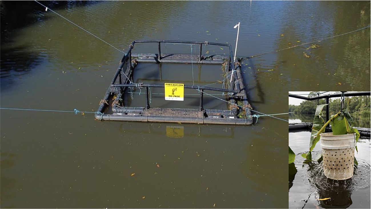
Figure 1. Floating cage where manatees where temporarily captured for recording (San San River, Bocas del Toro, Panama). Bucket filled with banana pulp and banana leaves used to attract the manatees (image insert).

The recordings of the 23 manatees in captivity yielded 1446 vocalizations (See Table 1). In the following section, we present the scheme used to obtain the vocalizations from the recordings.

Table 1

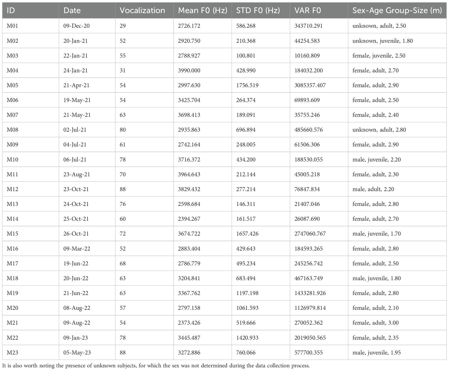
Table 1. Biological information and average acoustic features for each individual manatee.

2.2 Overview of manatee vocalization detection and identification

A data set was prepared by first extracting and then analyzing recorded manatee vocalization files using a detection scheme based on the works of Merchan et al (Merchan et al., 2019, 2020). The applied scheme (shown in Figure 2) consisted of a signal detection stage based on the analysis of the autocorrelation function (ACF) (Merchan et al., 2019), a denoising stage with the Smoothed Signal Subspace Denoising algorithm (Jensen et al., 2005) to eliminate noise, and a vocalization classification stage based on CNN (Merchan et al., 2020). During this classification stage, candidate signals identified in the detection stage are assessed using a CNN model that has been pre-trained to distinguishes between manatee vocalizations and other ambient noises. These steps correspond to the three first stages of the scheme presented in (Figure 2).

Figure 2

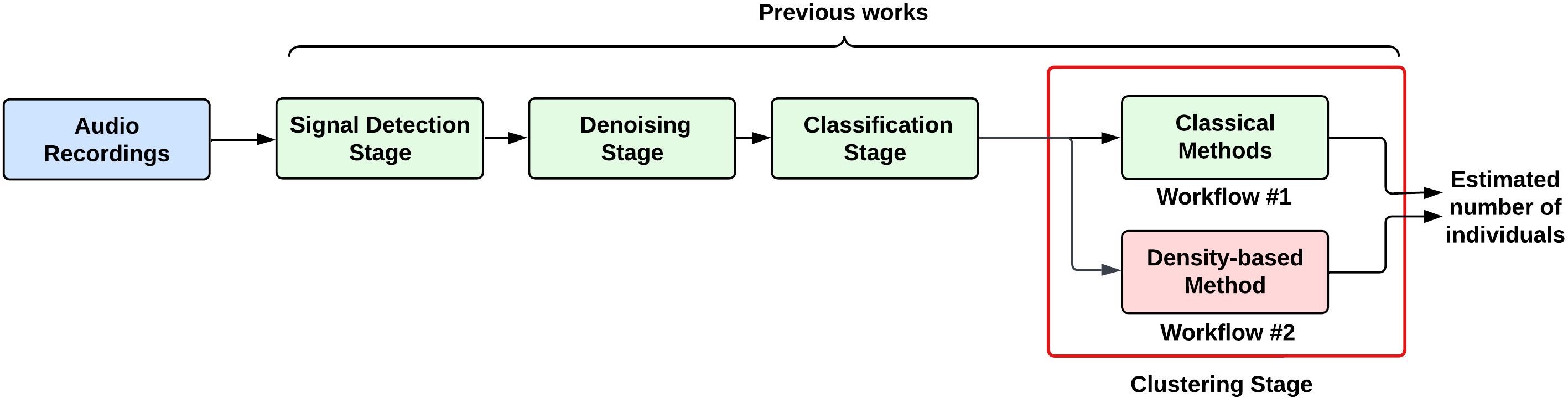
Figure 2. General description of the process of detection and identification of individual manatees. In the detection stage candidate manatee signals are extracted from recordings. Denoising stage enhances signal. In the classification stage, a trained model distinguishes between manatee vocalizations and other ambient noises. In the clustering stage, vocalizations exhibiting similar spectral properties are grouped together based on their acoustic features.

In Merchan et al. (2019), to estimate the number of individuals, the authors presented a “clustering stage” based on “classical clustering methods” such as K-means and hierarchical clustering. This approach used a STFT-based spectrograms and PCA for signal representation and dimensionality reduction, respectively. This approach will be called Workflow #1 throughout the text.

This workflow presented limitations that stemmed from its use of linear data representation through PCA and the clustering methods it employed, which posed challenges when handling data with nuanced similarities found in manatee vocalizations. Manatee vocalizations exhibit complexity, where individuals within similar demographics (such as same sex and age range) often present close fundamental frequencies and similar time-frequency contour properties. This affected the accuracy in the estimation of the number of manatees and the effective grouping of their vocalizations.

Taking advantages of a non-linear dimensionality reduction method and a density-based clustering methods to deal with this kind of data, we propose the Workflow #2, as an alternative for the Workflow #1 (see section 2.4).

2.3 Previous workflow

2.3.1 Overview of Workflow #1

The previous unsupervised learning framework, used as clustering stage, that is described in detail in Merchan et al. (2019) is depicted in Figure 3.

Figure 3

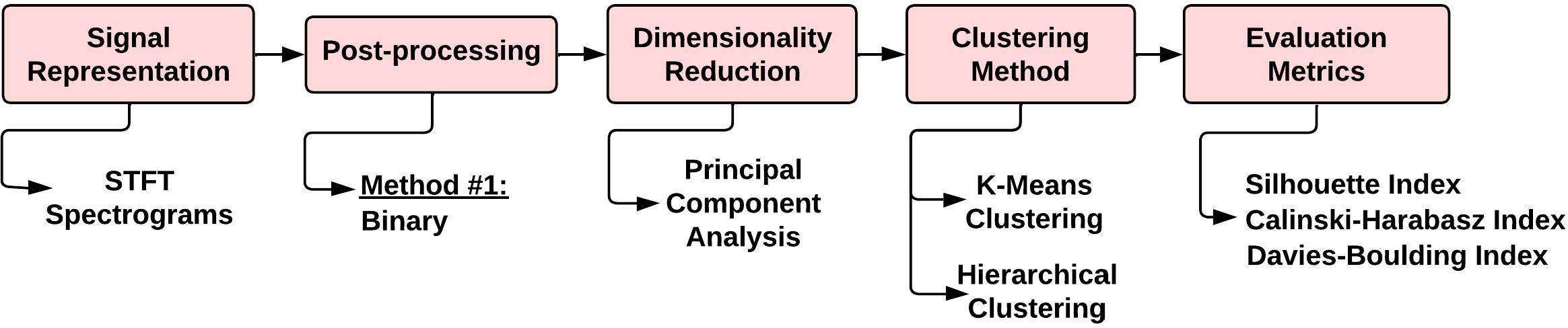
Figure 3. Diagram for Workflow #1. It comprises a signal representation stage using STFT spectrograms, a spectrogram post-processing stage, a dimensionality reduction stage by PCA, a clustering stage using classical methods (K-means or Hierarchical Clustering) and an Evaluation metrics stage.

It starts by generating STFT spectrograms and applying post-processing techniques (see Figure 4). Then, it uses PCA to reduce dimensionality for later grouping the data using two clustering methods (KM and HC). Finally, it evaluates the results employing internal validation metrics to find the optimal number of clusters.

Figure 4

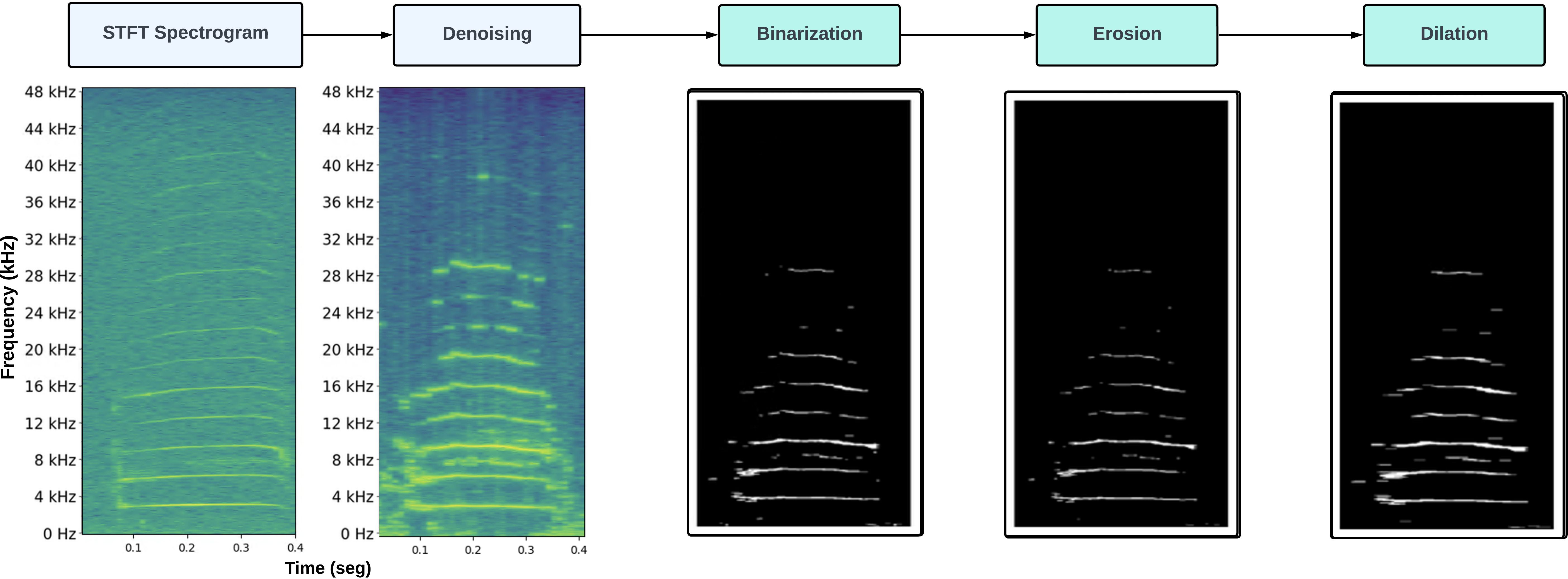
Figure 4. Spectrogram postprocessing. The signal spectrogram is denoised, binarized and subject to morphological operators of erosion and dilation.

2.3.2 Limitations of the STFT signal representation

We have found that the STFT Signal Representation have a few limitations when representing manatee vocalizations. The first one related to Heisenberg’s Uncertainty Principle. This principle indicates limitations between the frequency and time resolution of the representation, e.g. when the frequency resolution is increased, time resolution decreases and vice-versa.

Moreover, due to fixed window length and basis functions, the STFT does not entirely capture events with different duration or when the signal contains sharp sounds, diminishing resolution at higher frequencies (Beecher, 1988; Rajoub, 2020).

To find an optimal time-frequency trade-off, the Wavelet Transform utilizes special basis functions called “mother wavelets” that are not restricted to a single type of function (e.g., periodic functions as in STFT) and have both time and frequency components. This will generate a series of functions with different sizes and time-frequency spectrum (Rajoub, 2020).

2.3.3 Feature post-processing

Treating the spectrogram as a binary image allows to eliminate residual noise and highlight high energy harmonics. First, the values of input spectrogram are modified according to the binarization threshold, which will reduce to zero anything below n = 2 times the average value of the 2D array. Afterwards, morphological operators are applied to remove noise remnants using erosion with kernel size of (1,2) and then dilation to connect nearby regions and make them more contiguous with a kernel of size (1,4). Figure 4 provides a visual representation how STFT spectrograms are calculated.

2.3.4 Linear dimensionality reduction

According to Bellman and Kalaba (1965), “the curse of dimensionality” describes the rapid increase of computational complexity due to high volumes of numerical variables. In ML tasks, this is related to the scaling number of features used to train a model and its associated level of space and time complexity. In bioacoustics, a dataset of unprocessed feature-rich audio signals like animal vocalizations would not be immediately suitable for modelling, as perceptually similar sounds would not be located in a close neighborhood due to high dimensionality (Stowell and Plumbley, 2014).

To alleviate this problem, Dimensionality Reduction (DR) algorithms have been developed using mathematical tools to compress or reduce latent information without losing important features. Linear DR algorithms such as PCA (Turk and Pentland, 1991) have been used for this type of reduction due to their low computational complexity regarding bioacoustic analysis tasks (Odom et al., 2021). PCA attempts to linearly transform data into an orthogonal space where new features (named principal components) contain a percentage of the original data variance, and since the highest amount of variance is usually contained within the first few components, low variance features can be discarded. Nonetheless, despite having high efficiency for data compression, PCA and other linear algorithms are not able to capture complex nonlinear structure (Wang et al., 2020).

2.3.5 Internal clustering validation

In workflow #1 after, the dimensionality reduction, clusters are evaluated by different metrics. These metrics were chosen to evaluate different aspects of clusters in terms of inter-intra distance, this is, how individuals might differentiate one from another and how much vocalizations from one individual might differ. Each metric has its own set of thresholds that define whether a clustering result is optimal or not.

● Silhouette Index (SIL): It weights the inter-cluster and intra-cluster distance to calculate the score, ranging between -1.00 and 1.00. Higher scores indicate separated and well-defined clusters (Rousseeuw, 1987).

● Calinski-Harabasz Index (CAL): The score is higher when clusters are dense and well separated. For evaluation, it is computed in a heuristic manner. It measures data point dispersion at various degrees of freedom (i.e., by evaluating different centroids) (Caliński and Harabasz, 1974).

● Davies-Bouldin Index (DBI): The minimum score is zero, with lower values indicating better clustering. It uses the same heuristic approach as CH. The score is defined as the average similarity measure of each cluster with its most similar cluster, where similarity is the ratio of within-cluster distances to between-cluster distances (Davies and Bouldin, 1979).

The following subsection will present Proposed Workflow #2, which supersedes Workflow #1, by addressing methodologically some of the limitations described in this subsection.

2.4 Proposed workflow

2.4.1 Overview of Workflow #2

This new methodology starts by applying the Scattering Wavelet Transform (SWT) (Mallat, 2012). SWT is a time-frequency signal representation that provides superior time-frequency resolution compared to spectrograms based on the Short-Time Fourier Transform (STFT).

Then, a non-linear dimensionality reduction algorithm (also known as Manifold Learning) referred as PaCMAP (Pairwise Controlled Manifold Approximation) and described in (Wang et al., 2020), is used. It provides a better data representation in lower dimensions by capturing the complex data patterns inherent to manatee vocalizations without losing significant information in the process. Furthermore, to better distinguish the acoustic features of different individuals, we utilized a density-based clustering algorithm named HDBSCAN for Hierarchical Density-Based Spatial Clustering of Applications with Noise (Campello et al., 2013).

The proposed workflow for the clustering stage, is shown in Figure 5. First, instead of STFT, SWT coefficients are calculated to test different post-processing techniques (Figure 6). Then, dimensionality reduction is done using PaCMAP and finally HDBSCAN will attempt to find the best cluster number using the CDBw metric (noise and outliers are removed). Cluster quality is assessed using the same ground-truth metrics from workflow #1 (Figure 3).

Figure 5

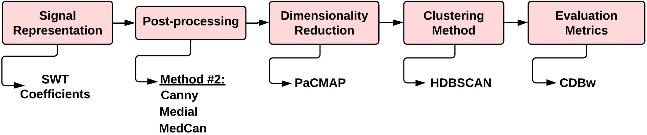
Figure 5. Diagram of the Workflow #2. It consist of a signal representation stage using SWT, a postprocessing stage, a dimensionality reduction stage using PacMAP, a clustering stage using HDBSCAN and an evaluation metrics stage.

Figure 6

Figure 6. Feature post-processing methods and their intermediary stages.

2.4.2 Improving feature extraction with Scattering Wavelet Transform

Considering the aforementioned requirements and limitations, we seek to test an approach that combines both the flexibility of wavelet functions and the effectiveness of neural networks to extract complex patterns, namely the Scattering Wavelet Transform. Proposed by Mallat (2012), it follows the concept of convolutional filters and non-linear activation functions, i.e., calculate a set of feature maps with prominent information and then find complex patterns.

Although the SWT behaves red similarly to CNNs, it provides an additional advantage, which entails minimal effort is spent in training and optimization. For further context, in situations where CNNs have been used for feature extraction, the neural network requires significant training data and computational processes (Rycyk et al., 2022). In the case of SWT, filter parameters that calculate optimal features are predefined by the characteristics of mother wavelet functions instead of being randomly initialized and learned from input data, making the SWT suitable for ML tasks (Oyallon et al., 2018).

In this work we used the implementation built by Andreux et al. (2020b). For this the SWT or S_Jx (Equation 1) is illustrated as a 3-layer cascade network of wavelet filters. The transform of input signal x(t) is defined as:

$\begin{array}{ll}{S}_{Jx}=\left[S_J^{(0)}x,S_J^{(1)}x,S_J^{(2)}x\right]& (1)\end{array}$

$\begin{array}{ll}{S}_J^{(0)}x=x\star {\varphi }_J(t)& (2)\end{array}$

$\begin{array}{ll}{S}_J^{(1)}x(t,\lambda )=\left|x\star {\psi }_{\lambda }^{(1)}\right|\star {\varphi }_J& (3)\end{array}$

$\begin{array}{ll}{S}_J^{(2)}x(t,\lambda ,\mu )=\left|\left|x\star {\psi }_{\lambda }^{(1)}\right|\star {\psi }_{\mu }^{(2)}\right|\star {\varphi }_J& (4)\end{array}$

In the above equations, the ⋆ operator denotes the convolution operation and || the non-complex modulus. While ${\psi }_{\lambda }^{(1)}$, ${\psi }_{\mu }^{(2)}$ and ϕ_J correspond to Morlet wavelet filters (with center frequencies at λ and µ) and a low-pass filter centered at the zero frequency. These parameters are controlled by two implemented parameters named Q and J, where Q controls the time-frequency resolution (number of wavelets per octave) and J the log-scale decomposition of the scattering transform, i.e., the number of times the signal is dilated and translated.

The SWT starts by computing $S_J^{(0)}x$ (zeroth-order coefficients, described in Equation 2). The local average of the signal which preserves most of the low frequency information, is then used to recover high frequency information, $S_J^{(1)}x$ and $S_J^{(2)}x$ as can be seen in (Equations 3, 4). They are also used to compute the first and second-order scattering coefficients, as depicted in Figure 7.

Figure 7

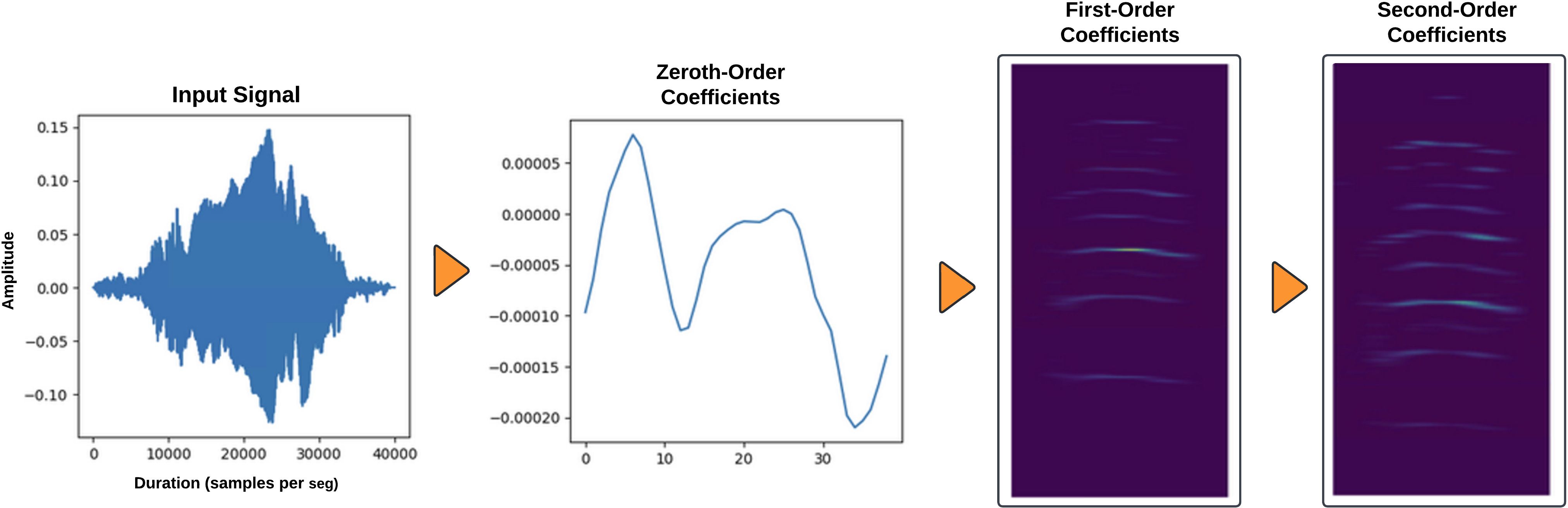
Figure 7. Stages of the scattering wavelet transform.

The modulus between layers acts like activation functions in neural networks, extracting non-linear patterns from convolved features. In addition, to the better preservation of high frequency components, other significant benefits of the SWT (in comparison to the STFT) are the reduction of variance and stability to additive noise and the deformation of the original signal (Mallat, 2012; Andén and Mallat, 2014).

2.4.3 Post-processing techniques

Similar to our previous work with STFT spectrograms (Merchan et al., 2019), described in section 2.3.3, it is necessary to normalize features for improved and consistent performance. Applying threshold binarization combined with morphological operators provided a suitable method to normalize Fourier coefficient values and remove noise artifacts. Nonetheless, this approach initially did not perform as well with SWT coefficients due to higher time-frequency resolution. Therefore, exploring additional combinations of image processing techniques produced a more fine-tuned representation of SWT coefficients. Three distinct techniques are sought to be tested, namely:

● The Canny Operator: Defined as an edge detection operator that employs a multi-stage algorithm to detect a wide range of edges in images (Canny, 1986), outperforms common operators and has been tested in conjunction with the Discrete Wavelet Transform for image filtering and noise reduction (Bachofer et al., 2016). In this work, it is used to find the edges of the spectral components of the SWT coefficients, and together with dilation and erosion operators, modify the shape and control the amount of resolution.

● Medial Axis Transform: An additional method to control and modify the SWT frequency components. The algorithm attempts to find a shape’s central “skeleton” or core of a shape, preserving its essential features (Lee, 1982).

● Medial Axis Transform with Canny Operator (MedCan): a combination of both methods designed to control both size and width of frequency components using the Medial Axis to find the bare minimum and Canny to increase resolution.

Using these techniques, combined with our previous binarization approach (section 2.3.3), the following feature transformation scheme was tested:

1. Generate a binary mask from the thresholded SWT coefficients (M times the mean value times, where M is pre-defined by the user).

2. Calculate the medial axis transform of the binary mask. This process can be repeated multiple times to achieve different levels of shape preservation, making frequency components thicker.

3. Create masked features by element-wise multiplication. Normalize features using min-max scaling, then re-adjust to 8-bit integer values.

4. Apply Gaussian Blurring to smooth features with a kernel size of (3,3). Blurring helps to reduce false positives by preventing the detection of small, noisy edges that may not be part of the actual structures in the image.

5. Calculate upper and lower hysteresis thresholds for the Canny algorithm. These parameters control which edges are considered true or not. After exploring more sophisticated methods (Liu et al., 2017) to determine these key parameters, the median value (md) of the input features and an arbitrary parameter σ (Equations 5, 6) were chosen to compute them automatically after experimenting with our dataset.

$\begin{array}{ll}{\text{Th}}_{\text{lower}}=\max (0,(1.0-\sigma )·\text{md})& (5)\end{array}$

$\begin{array}{ll}{\text{Th}}_{\text{upper}}=\min (255,(1.0+\sigma )·\text{md})& (6)\end{array}$

6. Apply dilation to connect nearby regions and make them more contiguous with a kernel of size (1,4).

7. Apply erosion to remove noise remnants with kernel size of (1,2).

For post-processing, different variations of the proposed method were tested (Figure 6), a visual representation of some of the key post-processing stages is included in this section (Figure 8).

Figure 8

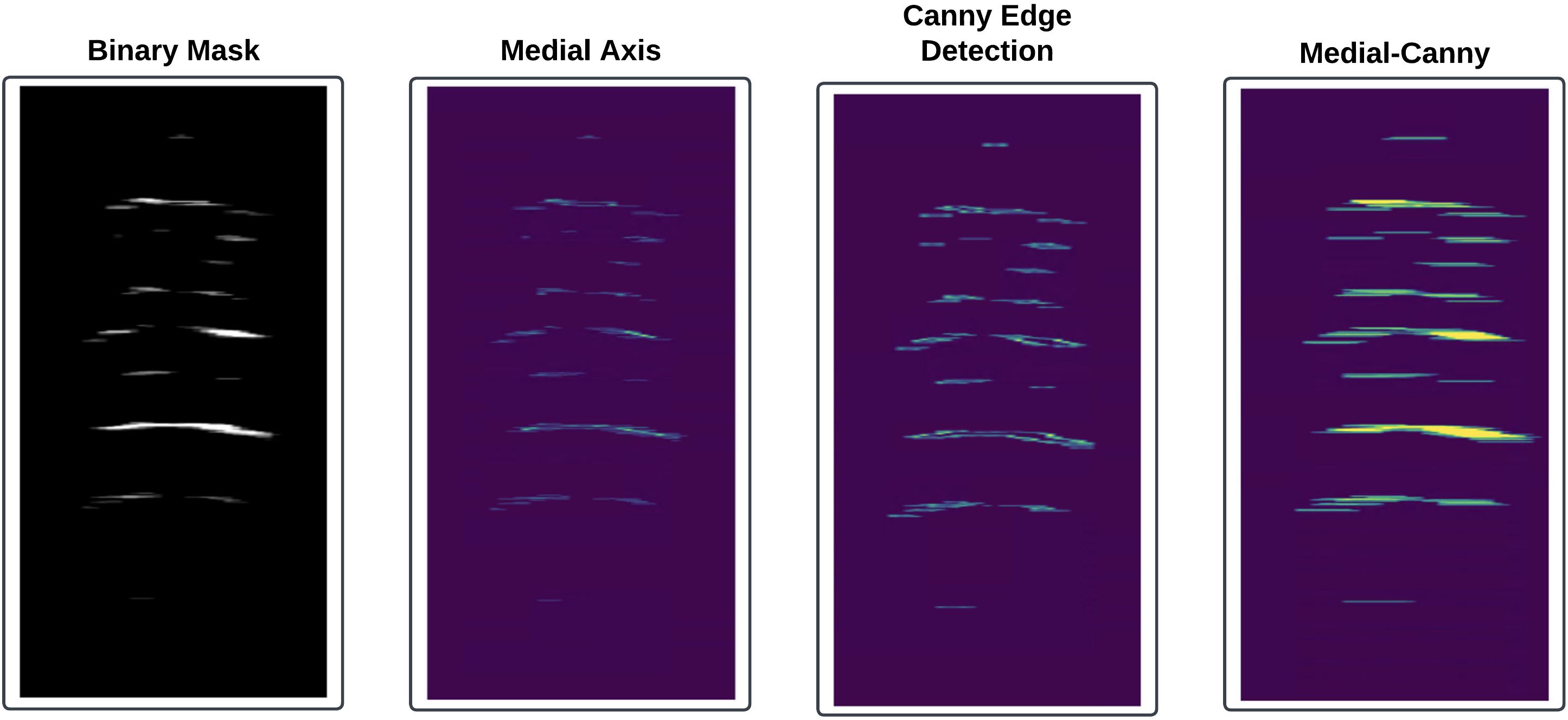
Figure 8. Post-processing techniques of SWT coefficients.

2.4.4 Non-linear dimensionality reduction

These methods classified as Manifold Learning, work in a holistic way by translating complex data onto a manifold (multidimensional geometric structure) in lower dimensions, while preserving intrinsic structure (original features) (Cayton, 2005). This has been achieved with different algorithmic approaches, where one of the most popular is t-SNE (t-distributed Stochastic Neighbor Embedding) (Van der Maaten and Hinton, 2008). This algorithm calculates a similarity measure between pairs of data points in both high and low dimensional space, then attempts to optimize them using a cost function to minimize the error rate. However, its performance is heavily reliant on proper parameter tuning to correctly model both local (observations very similar to each other) and global (observations very dissimilar to each other) structure, making it computationally expensive and unreliable for complex data analysis (Wang et al., 2020).

We experimented with PaCMAP, a Manifold Learning algorithm designed to capture global and local structure as accurately as possible with low computational complexity (requiring minimum parameter optimization). It effectively overcomes the limitations of preceding algorithms such as t-SNE (Wang et al., 2020). A simplified definition of the inner workings of the algorithm is as follows:

● Compute the weighted K-Nearest Neighbors graph (K-NN) (Eppstein et al., 1997) a data representation in high dimensions where each node represents similar observations (data points) and each edge represents the similarity between the data points. The algorithm can be initialized using PCA to reduce computational complexity without losing dimensionality reduction accuracy (Wang et al., 2020).

● Select smaller groups of data points by measuring similarity in terms of Euclidean distance. Then, three types of observation pairs (neighbor, mid-near and further pairs) will be considered to capture the global structure and then refine the local structure.

● Obtain a data embedding or representation in lower dimensions using of a cost function designed to minimize the error and preserve important latent features defined by the weighting scheme. This is done using the Adam optimizer, a popular algorithm in Deep Learning tasks (Kingma and Ba, 2014).

For this project, the PaCMAP software implementation developed by Wang et al. (2020) is used. It offers minimum parameter configuration to achieve optimal results. Empirical testing was done to find the best configuration between number of K-neighbors to consider for the K-NN graph initialization and the target dimensions of the resulting embedding.

2.4.5 Density-based clustering

Despite being computationally efficient and easily implemented, K-means and hierarchical clustering algorithms do not perform adequately when data points form clusters of variable size (i.e., varying degrees of similarity or density) nor with the presence of several outliers (Ahmed et al., 2020; Karim et al., 2021). In this work we tested the performance of HDBSCAN, a hierarchical density-based clustering algorithm that attempts to solve the previously mentioned limitations (Campello et al., 2013). It was developed as an extension of DBSCAN (Density-Based Spatial Clustering of Applications with Noise) presented by Martin et al. (1996).

DBSCAN clusters neighboring data points using a density threshold ϵ, to dictate how close they should be located to be considered part of a cluster with a predefined minimum size (a parameter defined as minPts), searching for the highest density regions to find suitable clusters. On the other hand, HDBSCAN will perform a cluster selection process when building a density-based hierarchy of various ϵ thresholds to account for clusters with different densities and shapes. This process will also eliminate noise data points and possible outliers by pruning data points and their neighbors that do not comply with the density criteria, established by how many neighboring points exists and how close they are.

We chose to use the HDBSCAN algorithm as McInnes et al. (2017) implemented. This algorithm will search for the best cluster configurations based on two key parameters: min_samples and min_cluster_size. The first one, similar to minPts in DBSCAN, determines the minimum number of samples required for a data point to be considered a core point, this is, a data point that has a certain minimum number of neighbors within its vicinity based on a specified distance measure such as Euclidean Distance. On the other hand, min_cluster_size sets the minimum size of clusters that the algorithm will identify.

2.4.6 Outlier detection

It is pertinent to include tools to refine clusters by eliminating data points with higher dissimilarity compared to their neighboring points within a specific region (local outliers) and global data points that fall outside the similarity range of the entire dataset (global outliers).

As part of the original HDBSCAN algorithm (Campello et al., 2013), Global-Local Outlier Score from Hierarchies (GLOSH) was implemented by Campello et al. (2015). Classified as a density-based outlier detection technique, it operates on the basis that non-outliers, are more likely to be discovered in densely populated areas while outliers can be found in low-density areas. When a data point deviates significantly from its closest neighbors (when it occurs far from its closest neighbors) it is marked and handled as an outlier (Wang et al., 2019). Hence, GLOSH is capable of simultaneously detecting both global and local outlier types based on a complete statistical interpretation.

The algorithm outputs an outlier score during the construction of the density-based hierarchy. It works by keeping track of parameters related to each data point, such as the first (last) cluster to which it belongs bottom-up (top-down) through the hierarchy, the lowest radius at which it still belongs to this cluster (and below which is labeled as noise), and the lowest radius at which this cluster or any of its sub-clusters still exist (and below which all its objects are labeled as noise) before being pruned during the cluster selection. The higher the score, the more likely the data point is to be an outlier (Campello et al., 2015). Therefore, pulling the upper quantiles from the outlier score distribution allows to identify and isolate data points in the higher range of the distribution.

2.4.7 Internal validation metrics for density-based models

For evaluating density-based clustering models, CDBw is a metric that indicates better performance when the index outputs high scores in a heuristic approach similar to CAL and DBI. It attempts to find the best cluster partition by measuring compactness in terms of density, which is, how close data points are to each other. Moreover, it can be tuned to use different distance metrics (Euclidean, Cosine, Correlation, among others) and uses an interval validation algorithm to handle noise data points (e.g., filtering, separate, combine, etc.) (Halkidi and Vazirgiannis, 2008).

2.5 Experimental setup

2.5.1 Data samples selection

To evaluate and compare the performance of each of the Workflows, the following experiments were design using randomly sampled subsets of the main dataset (Table 1):

● Experiment No. 1A - Random number of cluster test: In this experiment 100 datasets were generated by randomly keeping a range from 10 to 20 manatees of the global data set, selecting a random quantity of vocalizations for each individual with a range from 10 to 50 vocalizations. The purpose of this experiment is to measure the performance of each method in conditions where the ground truth is made of clusters of different sizes attempting to simulate a situation close to real life. Classical methods (i.e., KMC and HC) and density-based clustering approaches were compared with this dataset.

● Experiment No. 1B - Random number of cluster tests using mixed approaches: We interchange the representation methods of both workflows in this experiment. We tests the density-based clustering method and the dimensionality reduction (i.e, PacMAP) method of Workflow #2 with the Spectrogram STFT-based representation of Workflow #1. Also, we test the classical clustering methods and the dimensionality reduction method (i.e., PCA) of Workflow #1 with the SWT-based representation of Workflow #2. The purpose of this experiment is to determine the impact of the type of signal representation on the global performance of the workflows with respect the impact of the clustering and dimensionality reduction methods. In this experiment, we used the same datasets used in experiment No. 1A.

● Experiment No. 2 - Fixed number of clusters test: Following a similar protocol to the previous experiment, the best performing methods were subjected to further testing. In this case, 100 datasets were generated keeping a constant number of manatees (10 and 20) while varying the quantity of vocalizations between 30 to 50. For this experiment, only the density-based approach, HBDSCAN was considered.

● Experiment No. 3 - Full dataset test: In this test, we carry out clustering of the whole dataset with the Workflow #2.

2.5.2 Clustering methods settings and configuration

We present the settings and configurations of the compared clustering methods of both workflows:

● Classical clustering methods presented in Merchan et al. (2019), K-Means Clustering (KMC) and Hierarchical Clustering (HC): For these methods, the dimensionality reduction was done using PCA.

● For all experiments, classical clustering methods were evaluated for 10 to 20 clusters iterating between 3 PCA configurations (accounting for 70, 80 and 90% of cumulative variance) and the aforementioned internal validation metrics (SIL, DBI and CAL) to select the optimal clustering.

● Density-based method, HBDSCAN: For this method, the dimensionality reduction was done using the Manifold Learning algorithm, PaCMAP. The HBDSCAN implementation had the following specifications:

● Embedding dimensions: From 5 to 9. It is worth mentioning that above 9 dimensions, the algorithms start outputting diminishing returns in terms of clustering quality in relation to scaling computational complexity.

● KNN-graph: The K parameter related to the number of k-nearest neighbors used to build the graph representation in higher dimensions was iterated from 4 to 6.

● Minimum samples and cluster: Fixed size of 10 and 15.

● For CDBw evaluation: Manual experimentation showed that the cosine distance was the best compared to the standard Euclidean distance. Moreover, the internal validation algorithm was set to filter noise data points (i.e., vocalizations that were labeled numerically as −1 by HDBSCAN) before evaluation.

● Outlier detection: All experiments were set to pull the 80th percentile of outlier scores, this is, identify the top 20% of data points with the highest scores and classify them as outliers.

2.5.3 Signal representation parameters

● Binary spectrograms: They were generated using 2048 NFFT bins with 50% overlap and Hanning Window function, resulting in 1024x150 zero-padded spectrograms after binarization (with a threshold equals to 2 times the mean value of each vocalization) with kernel sizes of 2 and 4 (for erosion and dilation operators respectively).

● SWT second-order coefficients: They were generated with J=10 and Q=100 resulting in 2D arrays of 3049x200 features. The binarization threshold was kept at 20 times the mean array value for all experiments.

In this work, the impact of different post-processing methods in clustering performance was evaluated by comparing the previous STFT (Merchan et al., 2019) against the proposed SWT, using different variations to find the best signal representation.

2.5.4 External validation metrics

According to Liu et al. (2010), clustering results can be evaluated using two different sets of metrics: unsupervised without ground truth (internal validation) or with the supports of ground truth labels (external validation).

Since manually annotated labels were available in this work, the V-Measure (Rosenberg and Hirschberg, 2007) (VM) external validation metric was utilized to measure how many manatees can be identified with unsupervised methods. Using two criteria, this metric compares the ground truth against generated cluster labels to determine the clustering quality. Homogeneity (hereafter, H) which measures data point similarity within a cluster, and completeness (hereafter, C) which calculates how many similar data points are clustered by the algorithm. The VM score is the harmonic mean between C and H scores (Rosenberg and Hirschberg, 2007).

Additionally, the Fowlks-Mallows Index (hereafter, FMS) quantifies the similarity between two sets of cluster labels, providing insights into how many samples are being clustered correctly and is defined as the geometric mean of the pairwise precision and recall (Fowlkes and Mallows, 1983). All these metrics output values between 0 and 1.00, where 1.00 indicates perfect cluster composition between 2 sets of labels (VM Score) and perfect accuracy (FMS).

Furthermore, it is necessary to evaluate not only the quality of the clusters but also the quantity of estimated clusters compared to assigned individuals (ground truth). For this task, the following proposed metrics by are the Mean Absolute Error Clusters Number Estimation (MAECNE) and Mean Percentage Error Cluster Number Estimation (MPECNE%) that were calculated as follows (Equations 7, 8):

$\begin{array}{ll}\text{MPECNE\%}=\overline{\left|\frac{\text{Estimated\hspace{0.17em}Number\hspace{0.17em}of\hspace{0.17em}Clusters}-\text{True\hspace{0.17em}Number\hspace{0.17em}of\hspace{0.17em}Clusters}}{\text{True\hspace{0.17em}Number\hspace{0.17em}of\hspace{0.17em}Clusters}}\times 100\right|}& (7)\end{array}$

$\begin{array}{ll}\text{MAECNE}=\overline{\left|\text{Estimated\hspace{0.17em}Number\hspace{0.17em}of\hspace{0.17em}Clusters}-\text{True\hspace{0.17em}Number\hspace{0.17em}of\hspace{0.17em}Clusters}\right|}& (8)\end{array}$

These metrics described in Equations 7, 8 are obtained by averaging over a fixed number of experiments in a particular setting. Finally, we introduce another performance metric defined as Percentage Cluster Quality (PCQ%). This metric is used to evaluate the composition of each cluster and determine how many manatees have been successfully identified, it follows this set of steps:

1. Calculate the composition of each cluster in terms of percentage per individual.

2. Find the dominant individual with the highest percentage of vocalizations for each cluster.

3. Average the percentage of all dominant individuals in each obtained cluster.

After computing all clustering iterations, the resulting labels were evaluated using external validation (H, C, V and FMS) and performance metrics (MAECNE, MPECNE% and PCQ%) to determine the cluster quality using the ground truth as reference (See Tables 2–5).

Table 2

Table 2. Results for Experiment No.1A: Comparison of Workflow #1 and Workflow #2 using all the variants of internal validation metrics and signal representation.

Table 3

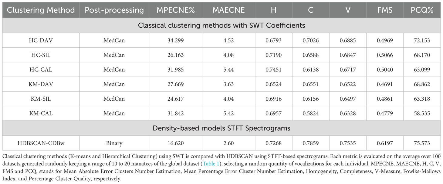
Table 3. Results for Experiment No.1B of mixed approaches.

Table 4

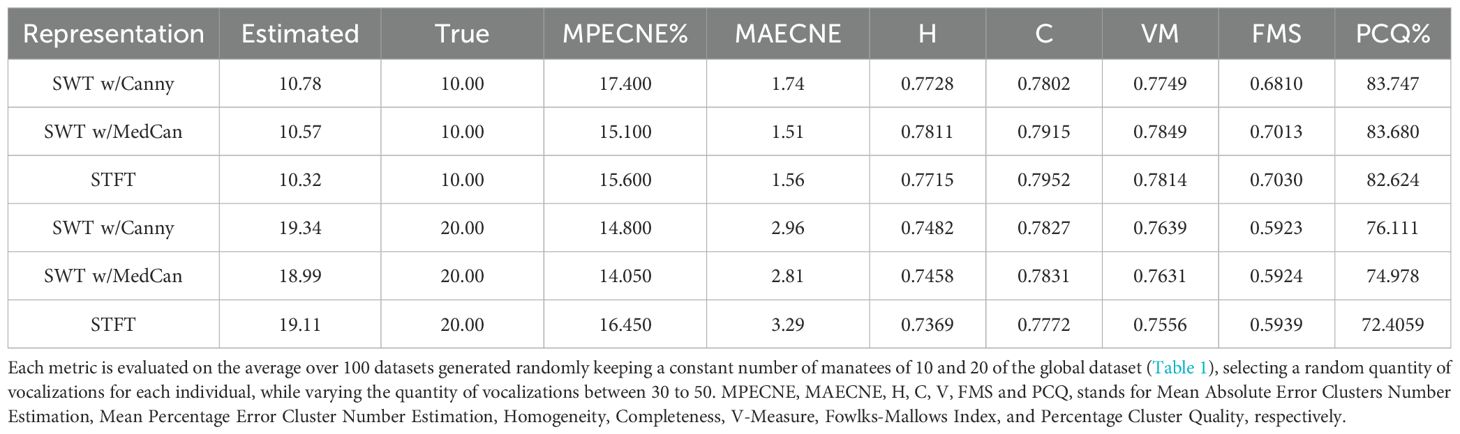
Table 4. Results of Experiment No. 2 - Evaluation of HDNSCAN clustering method three signal representation options: SWT with Canny, SWT with MedCan and STFT.

Table 5

Table 5. Results of Experiment No.3 - Clustering performance Workflow #2 over the full data set (Table 1).

2.5.5 Cluster quality analysis

The experiment No.3 was conducted using the entire dataset (Table 1) to study cluster quality and identify biological features that could impact identification performance. The analysis consist of the following aspects:

● Acoustic analysis: Fundamental frequency, also known as pitch, is the key parameter that has been showed to be related to demographic features of interest such as sex or age (Sousa-Lima et al., 2002, 2008; Umeed et al., 2018; Brady et al., 2022). In this work, the Probabilistic YIN algorithm (PYIN) provided a reliable way to calculate the fundamental frequency of each vocalization. Developed from the original YIN algorithm (De Cheveigné and Kawahara, 2002), is a pitch estimation method that computes the difference between the signal and delayed versions of itself (in a similar fashion to a window analysis using the ACF function) to find the most probable frequency (F0) among a set of candidates.

● Unlike the original algorithm, it does not require a threshold parameter to filter out noise frequencies and is more suited to analyze complex harmonic signals such as the manatee vocalizations (Mauch and Dixon, 2014). To obtain better results and filter noise artifacts, the algorithm’s parameters were configured to analyze frequencies located between the seventh and eight octave of the musical chromatic scale (between 2.093 and 7.902 kHz), corresponding to the manatee’s vocal pitch (Brady et al., 2022).

● Cluster embedding analysis: We consider that the more compact a cluster is depicted in the embedding space, the more similar its features should be. We used the Convex Hull (CH) to verify this idea (Preparata et al., 1985).In computational geometry, CH is defined as the outer boundary of a set of data points and can be used to characterize a cluster by encapsulating the extent of its points in Euclidean space.

After obtaining a set of post-processed clusters (without noise samples and outliers), the CH of each cluster was computed, and its volume was computed. By using this parameter as a reference, clusters can be arranged from higher to lower volume and then. It can be observed which individuals are identified in homogeneous clusters and which tend to be mixed. This parameter, together with other acoustic and biological features such as F0, animal size, and sex, could provide insights regarding the strengths and weaknesses of our current methods to cluster vocalizations of manatees.

2.5.6 Computational hardware and software

All experiments were performed using a custom PC with AMD Ryzen 9 5950X CPU processor and 64GB of RAM running on Ubuntu 22.04 kernel. This includes Python libraries such as Numpy, Scikit-learn, Librosa, OpenCV and Scipy. For the core algorithms of the new methodology we utilized the following repositories made by Wang et al. (2021) (https://github.com/YingfanWang/PaCMAP), Leland McInnes and Astels (2017) (https://github.com/scikit-learn-contrib/hdbscan), and Andreux et al. (2020a) (https://github.com/kymatio/kymatio).

3 Results

3.1 Clustering performance

As mentioned, different experiments were devised to assess the behavior of both workflows. Tables 2, 3 show the results regarding the Experiment No.1A and 1B using a random number of clusters, with each column corresponding to the average best scores and metrics after fitting all models for all 100 datasets. We emphasize that each model was evaluated with the same randomly generated hundred data sets (n=100).

One can observe that, in general, the density-based clustering approach, HBDSCAN, presented the best metrics in all the categories. Indeed, when using the STFT Spectrogram representation, it obtained a Mean Percentage Error of Cluster Number Estimation (MPECNE) of 16.620% (Table 3), followed closely by the results for the SWT Canny and MedCan variants, with 19.268% and 18.479%, respectively (Table 2). Both classical clustering methods (KM and HC) obtained values above 27.617% for MPECNE.

Also, the best external evaluation metrics were obtained for HBDSCAN, with values reaching 0.7437 for Homogeneity (H), 0.8002 for Completeness (C), 0.7691 for V-Measure and 0.6387 for FMS. On the other hand, these metrics for the classical clustering approaches (KMC and HC) were below the scores. Also, HBDSCAN obtained the highest value for the Percentage Cluster Quality (PCQ), which measures the percentage of the dominant manatee in a cluster on average, reaching 77.282% for the SWT MedCan variant (Table 2).

Table 3 shows the results of Experiment No.1B. One can conclude that the choice of clustering methods and the dimensionality reduction method play a larger role in the results, than the type of representation signal since the HDBSCAN clustering using STFT spectrogram provides a better results that HC and KM methods using SWT.

Moreover, Table 4 shows the result of Experiment No. 2, with a fixed number of clusters (10 and 20 clusters) using a density-based clustering approach, HDBSCAN for the variants with best metrics scores of Experiment No.1., SWT Canny and MedCan and the STFT Spectrogram. Scores for these variants are very close for most metrics, with a slightly best score for Mean Percentage Error Cluster Number Estimation for MedCan with 15.100% for 10 clusters and 14.050 for 20 clusters, while the best scores of Percentage Cluster Quality were obtained by the Canny variant, reaching 83.747% for 10 clusters and 76.111% for 20 clusters.

3.2 Cluster quality analysis of the full dataset (Experiment No.3)

Results of Experiment No. 3 are shown in Table 5. Here, the complete dataset was analyzed using HDBSCAN with the Canny variant. The Canny variant was chosen due to its higher performance compared to Medial and very similar performance compared to MedCan in Experiment No.1A and No.2.

For the 23 true clusters, the estimated number of clusters was 24 (MPECNE of 4.34%) and the Percentage Cluster Quality reached 78.453%. V-Measure reached 0.8457 and the FMS reached 0.7852.

After computing dimensionality reduction and clustering stages with PaCMAP and HDBSCAN, the cluster labels were used to generate Tables 6, 7, which showed the results when compared against the observed cluster conformation (ground truth). For both Tables 6, 7, rows were organized in ascending order according to each cluster Convex Hull volume, which was automatically calculated in an earlier step. In Figure 9 the composition of clusters presented in Table 6 are illustrated using stacked bars.

Table 6

Table 6. Composition of the obtained clusters of the Experiment #3 in terms of the ground truth labels of manatee vocalizations.

Table 7

Table 7. Biological features organized per individual for each cluster in Experiment No.3 - Full dataset.

Figure 9

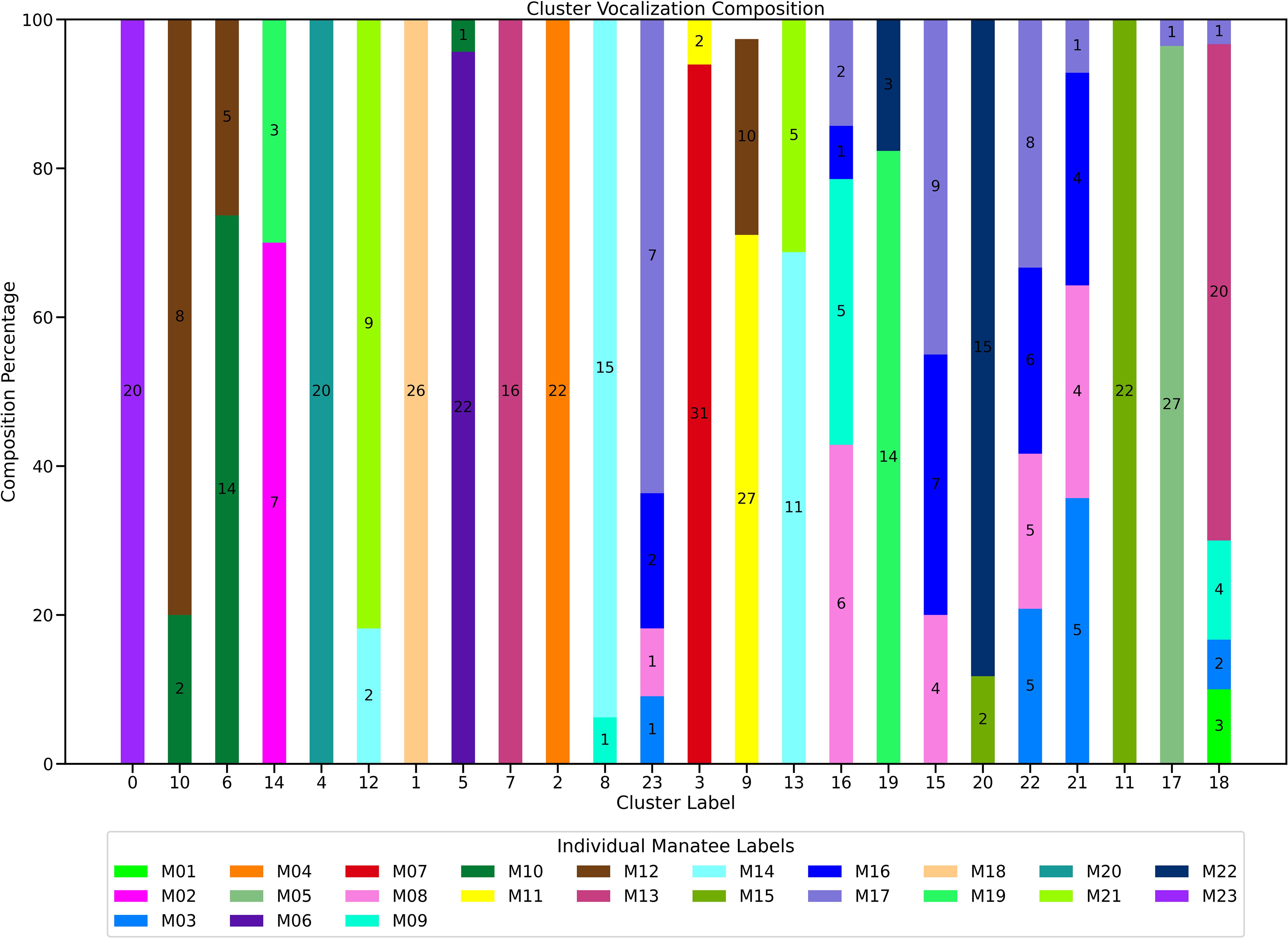
Figure 9. Graphical representation of the percentage composition of individual manatees in each cluster as per Table 6. Clusters are arranged in the order of Table 6 (ascending order based on their convex hull). Each manatee is represented by a specific color (refer to the legend at the bottom), with the number of vocalizations per individual displayed for each bar.

To further explain this comparison, Figure 10 shows the embedding with just ground truth labels. Figure 11 shows the obtained clusters from HDBSCAN. For contrast, the clusters found are shown in color, and while noise is shown in black.

Figure 10

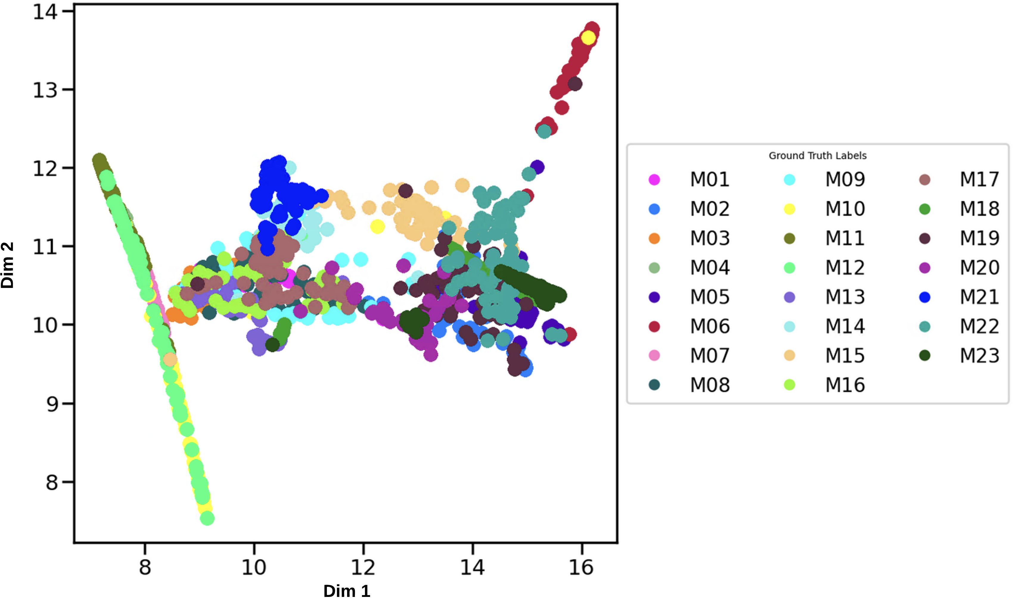
Figure 10. Full embedding with ground truth labels showing the vocalizations of the 23 manatee individuals (Experiment No.3). Each point of the diagram corresponds to a vocalization of the dataset. manatee. Each manatee is assigned a different color as indicated in the legend at the right, from M01 to M23.

Figure 11

Figure 11. Full embedding of the clusters obtained by the HDBSCAN clustering algorithm in Experiment No.3. Each cluster corresponds to the estimated group of vocalizations of an individual manatee. For each of the obtained 24 clusters, a color is assigned as indicated in the legend at the bottom, from C0 to C23. The left panel shows the clusters in color and noise in black. The right panel shows filtered embedding (no noise or outliers).

Furthermore, Figure 12 shows the top five (5) clusters with minimum convex hull coverage obtained using the HDBSCAN, that is, clusters with high cohesion. While Figure 13 shows the bottom five (5) clusters with maximum coverage, thus a higher spread.

Figure 12

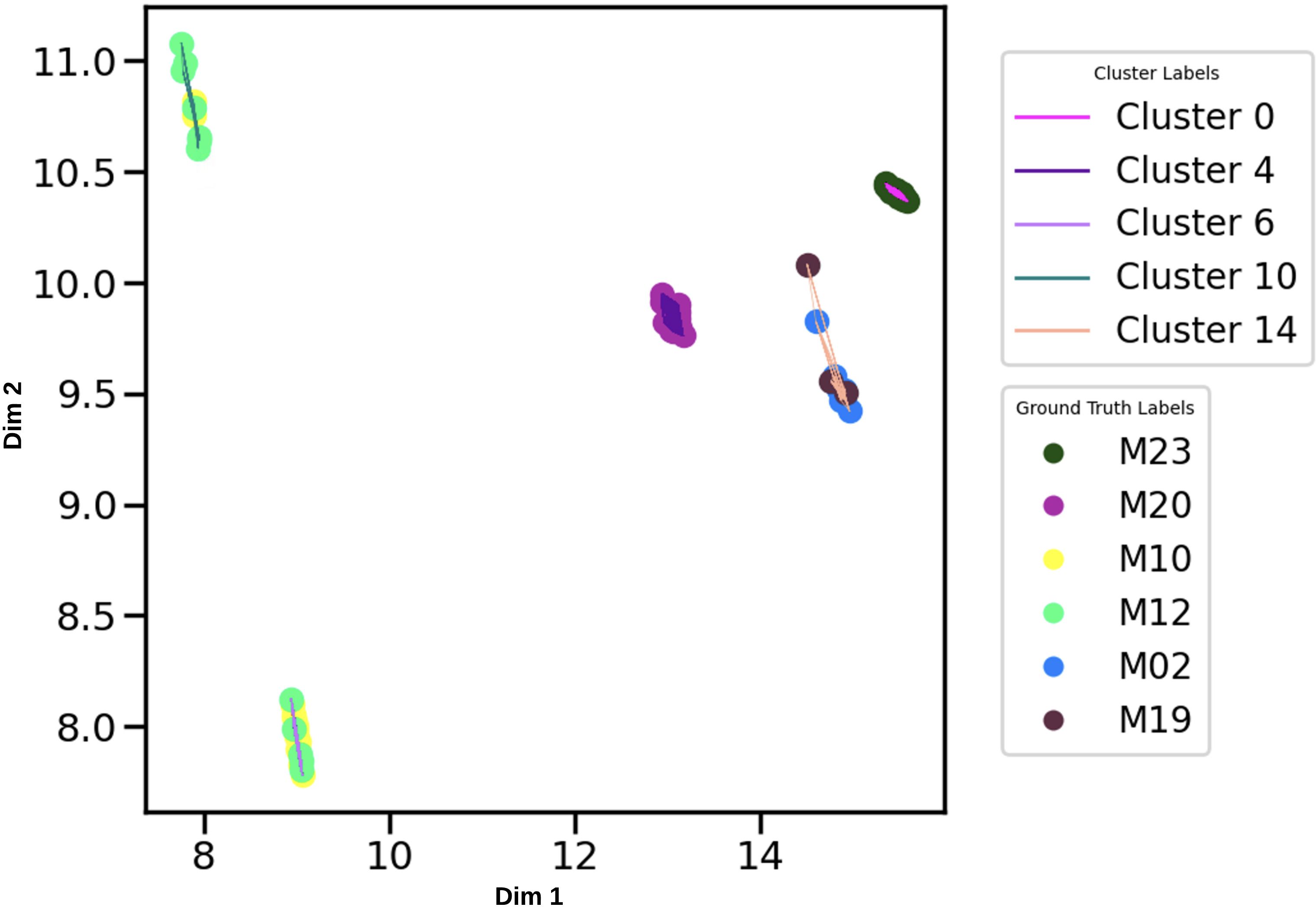
Figure 12. Filtered embedding for the 5 obtained clusters with minimum Convex Hull (CH) volume (top 5 clusters in Table 6, Clusters: 0, 4, 6, 10, and 14). For each of the 5 clusters, colored line is assigned as indicated in the legend at the top right (same colors used in Figure 11). Vocalizations of manatees in these clusters are presented as points with different colors as indicated in the legend at bottom right (same colors used in 9).

Figure 13

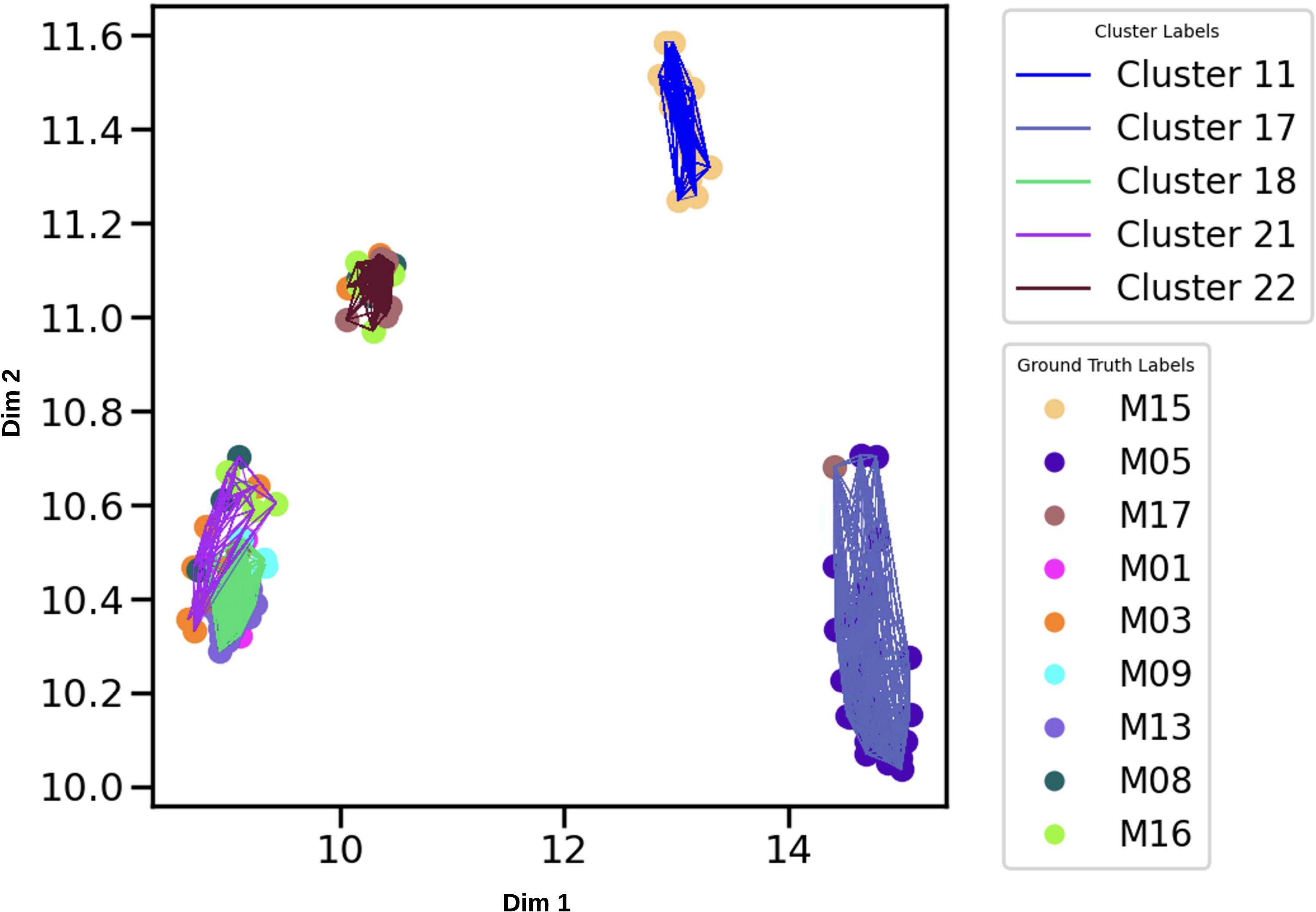
Figure 13. Filtered embedding for the 5 obtained clusters with maximum Convex Hull (CH) volume (bottom 5 clusters in Table 6, Clusters: 11, 17, 18, 21 and 22). For each of the 5 clusters, the colored line is assigned as indicated in the legend at top right (same colors used in Figure 11). Vocalizations of manatees in these clusters are presented as points with different colors as indicated in legend at bottom right (same colors used in 9).

Finally, Table 7 shows the biological information reorganized from Table 1 and the average vocalization F0 per individual on each cluster.

4 Discussion

This work compares two clustering methods for identifying the Greater Caribbean manatee. This continues the group’s work and builds upon previous works (Merchan et al., 2019) oriented towards unsupervised learning of manatee vocalizations. The newly proposed method is based on density clustering (HDBSCAN), and outperforms previously used clustering methods (KM and HC). It does so by providing an increased performance, between 10 and 20%, in most evaluation metrics according to external validation (Table 2). It is important to remark that more than half of the post-processing variants (SWT and STFT spectrogram representations) had close performance metrics across the board. Hence, later results are only presented with the Canny variant for the cluster quality test.

According to results in Experiment No.2, HDBSCAN using SWT presented a better performance in terms of both MPECNE and PCQ. This is probably due to the improved feature extraction capability granted by the SWT. Indeed, as mentioned earlier, SWT, by incorporating principles related to neural networks, such as the hierarchical feature scheme (denoted by the 2 layers of wavelet filters), work similarly. This without implementing a complex neural network training schema with learned features (pre-computed wavelet filter frequencies). This approach allows to obtain more fine-grained time-frequency resolution with less information loss in the high frequencies due to the versatility of wavelet filters (see Figure 7). Basically, the same vocalization is presented with additional harmonics in the upper frequencies in the post-processed SWT coefficients, when compared to STFT binary spectrograms.

Regarding the capability of identifying the number of clusters and its closeness to the ground truth (number of individuals manatee in a dataset), we observe the lowest error rate is achieved in Experiment No.1 with, HBDSCAN as the clustering method, with 16.620%, while the classical clustering methods (KM and HC) reached 27.617%, a difference of almost 10%. These results can be translated into the rounded capability of identifying ±3 or ±5 clusters depending on the method MAECNE scoring. Moreover, the homogeneity of such clusters can get as high as 0.7437 (HBDSCAN) compared to with 0.7451 using classical clustering methods with SWT. In terms of %PCQ, the average quality of such clusters can reach 77.282% with HBDSCAN (using MedCan post-processing) compared to 72.153% from HC using SWT with DAV evaluation metric (Table 2).

In general, the results of experiments No.1 and No.2 provide insights into the minimum expected performance in pseudo-random circumstances and the order of magnitude of error in relation to the number of vocalizations per cluster. This is confirmed when one looks at the resulting number of vocalizations per cluster, 10-50 and 30-50 for Experiment No.1, and No. 2, respectively.

Regarding the anticipated performance of our approach across various natural sound environments, selecting appropriate denoising methods and settings is crucial. Depending on the specific acoustic conditions present in each location, we employ techniques such as signal subspace, spectral subtraction, or Wiener filters (Ephraim and Trees, 1995). In general, when selecting the appropriate denoising approach and settings, the proposed approach obtained expected performance.

For the case of Experiment No. 2, where the number of possible manatees is kept constant and the number of vocalizations per cluster is in the 30 to 50 range, a decreased error rate of between 17.4 and 14.05% can be observed (%MPECNE in Table 4). This is further improved in Experiment No. 3 with the full dataset test (Table 5) where the error rate decreases even further, to 4.3%. Moreover, regarding of absolute error (MAECNE), the rounded identification capability stands between ±2 and ±3 with reduced ground truth clusters. This includes a homogeneity ranging between 0.7482 and 0.7811 (when analyzing datasets of 10 and 20 individuals) and as high as 0.8479 with the full dataset (Table 5).

Regarding the cluster quality analysis from Experiment No. 3, when organizing rows in ascendant order showed that most of the clusters with high quality are located in the upper rows, while the opposite happens for lower quality clusters. This occurrence can be observed in the convex hull plot, where very compact clusters are presented in Figure 12 and spread clusters in Figure 13.

However, four clusters of high quality are located in the lower rows, these correspond to the individual manatees with highest F0 variance (M05, M15, M19 and in Table 1). This could indicate that the Convex Hull volume could be used as a tool to evaluate cluster homogeneity in conjunction with additional tools to confirm that, although with a high volume, a cluster might belong to individuals with higher pitch variance.

In Figure 14 we can observe several vocalizations of a male juvenile (M15), a male adult (M12) and a female adult (M20). For instance, the male juvenile (M15) presents a high F0 variance. However, high F0 variance in also found in three female adults (M05, M19, M22). In the Supplementary Materials, spectrograms for each manatee in the database are presented.

Figure 14

Figure 14. Examples of vocalizations from juvenile, male and female individuals.

Furthermore, examining the cluster composition reveals that most clusters share common sexes and ages across individuals (e.g., clusters with only female adults or clusters with only male juveniles). However, in some cases we observed that some vocalizations of juvenile males are found in clusters where the dominant individual is a female, but both have a very similar F0 (M06 in Cluster 5), and another similar case where the dominant individual is a female (M11 in Cluster 9) while the rest of vocalizations belong to high pitch males, one of them being a juvenile.

5 Conclusions

In this paper, we proposed a new methodology for manatee identification and counting using vocalizations of underwater recordings through a clustering algorithm. This methodology serves as a tool for estimating of manatee populations acoustically. The methodology uses Scattering Wavelet Transform for signal representation, a non-linear dimensionality reduction algorithm, PaCMAP and a density-based clustering approach called HBDSCAN. This methodology obtained better results than a previous methodology presented by the authors using STFT spectrograms, PCA (a linear dimensionality reduction method) and classical clustering algorithms (K-means and Hierarchical clustering). The proposed methodology a reaches mean percentage of error estimating the number of individuals in a dataset of 14.05% and a success of correctly grouping the vocalizations manatee in a cluster of 83.75%. Further modeling should refine the interpretation of age and gender vocalizations classes for demographic studies.

Data availability statement

The raw data supporting the conclusions of this article will be made available by the authors, without undue reservation.

Ethics statement

The animal study was approved by Animal Care and Use Committee (ACUC), Smithsonian Tropical Research Institute (STRI). The study was conducted in accordance with the local legislation and institutional requirements.

Author contributions

FM: Conceptualization, Funding acquisition, Investigation, Methodology, Project administration, Resources, Supervision, Writing – original draft, Writing – review & editing. KC: Conceptualization, Data curation, Investigation, Methodology, Software, Visualization, Writing – original draft, Writing – review & editing. HP: Conceptualization, Investigation, Resources, Writing – original draft, Writing – review & editing. HG: Conceptualization, Data curation, Funding acquisition, Investigation, Methodology, Project administration, Resources, Supervision, Validation, Writing – original draft, Writing – review & editing. JS-G: Conceptualization, Data curation, Investigation, Methodology, Resources, Software, Supervision, Visualization, Writing – original draft, Writing – review & editing.

Funding

The author(s) declare financial support was received for the research, authorship, and/or publication of this article. This research was supported by the Secretaría Nacional de Ciencia Tecnología e Innnovacion (SENACYT-Panama) through contracts FID18-76, FID21-90, and FID23-106, and the Smithsonian Tropical Research Institute (STRI). The Sistema Nacional de Investigación (SNI), SENACYT-Panama supports research activities by FM, HP, JS-G, and HG.

Acknowledgments

We thank Jossio Guillen for unconditional field assistance and logistical support. We thank Alfredo Caballero and Roberto Gonzalez for their help installing the pen and Candy Real for providing transportation support. We also thank the board of AAMVECONA for renting access to the pier and electricity to observe the manatees. We thank the board of COOBANA R. L. banana company, particularly Chito Quintero, Diomedes Rodriguez and Dinora Beitia, for providing banana fruits at no cost for over two years. The authors acknowledge administrative support provided by CEMCIT-AIP, STRI and Universidad Tecnológica de Panamá (UTP).

Conflict of interest

The authors declare that the research was conducted in the absence of any commercial or financial relationships that could be construed as a potential conflict of interest.

Publisher’s note

All claims expressed in this article are solely those of the authors and do not necessarily represent those of their affiliated organizations, or those of the publisher, the editors and the reviewers. Any product that may be evaluated in this article, or claim that may be made by its manufacturer, is not guaranteed or endorsed by the publisher.

Supplementary Material

The Supplementary Material for this article can be found online at: https://www.frontiersin.org/articles/10.3389/fmars.2024.1416247/full#supplementary-material.

References

Ahmed M., Seraj R., Islam S. M. S. (2020). The k-means algorithm: A comprehensive survey and performance evaluation. Electronics 9, 1295. doi: 10.3390/electronics9081295

Crossref Full Text | Google Scholar

Andén J., Mallat S. (2014). Deep scattering spectrum. IEEE Trans. Signal Process. 62, 4114–4128. doi: 10.1109/TSP.2014.2326991

Crossref Full Text | Google Scholar

Andreux M., Angles T., Exarchakisgeo G., Leonardu R., Rochette G., Thiry L., et al. (2020b). Kymatio: Scattering transforms in python. J. Mach. Learn. Res. 21, 2256–2261.

Google Scholar

Andreux M., Exarchakis G., Leonarduzzi R. F., Angles T. (2020a). Kymatio:wavelet scattering transforms in python with gpu acceleration. Journal of Machine Learning Research. 21 (60), 1–6.

Google Scholar

Aragones L., Lawler I., Marsh H., Domning D., Hodgson A. (2012). “The role of sirenians in aquatic ecosystems,” in Sirenian Conservation (University Press of Florida, Florida USA), 4–11. doi: 10.2307/j.ctvx079z0

Crossref Full Text | Google Scholar

Bachofer F., Quénéhervé G., Zwiener T., Maerker M., Hochschild V. (2016). Comparative analysis of edge detection techniques for sar images. Eur. J. Remote Sens. 49, 205–224. doi: 10.5721/EuJRS20164912

Crossref Full Text | Google Scholar

Beecher M. D. (1988). Spectrographic analysis of animal vocalizations: implications of the “uncertainty principle. Bioacoustics 1, 187–208. doi: 10.1080/09524622.1988.9753091

Crossref Full Text | Google Scholar

Bellman R., Kalaba R. E. (1965). Dynamic programming and modern control theory Vol. 81 (Pennsylvania State University: Citeseer).

Google Scholar

Brady B., Ramos E. A., May-Collado L., Landrau-Giovannetti N., Lace N., Arreola M. R., et al. (2022). Manatee calf call contour and acoustic structure varies by species and body size. Sci. Rep. 12, 19597. doi: 10.1038/s41598-022-23321-7

PubMed Abstract | Crossref Full Text | Google Scholar

Caliński T., Harabasz J. (1974). A dendrite method for cluster analysis. Commun. Statistics-theory Methods 3, 1–27. doi: 10.1080/03610927408827101

Crossref Full Text | Google Scholar

Campello R. J., Moulavi D., Sander J. (2013). “Density-based clustering based on hierarchical density estimates,” in Advances in knowledge discovery and data mining (Berlin, Heidelberg: Springer), 160–172.

Google Scholar

Campello R. J., Moulavi D., Zimek A., Sander J. (2015). Hierarchical density estimates for data clustering, visualization, and outlier detection. ACM Trans. Knowl. Discovery Data (TKDD) 10, 1–51. doi: 10.1145/2733381

Crossref Full Text | Google Scholar

Canny J. (1986). A computational approach to edge detection. IEEE Trans. Pattern Anal. Mach. Intell. PAMI-8, 679–698. doi: 10.1109/TPAMI.1986.4767851

Crossref Full Text | Google Scholar

Cayton L. (2005). Algorithms for manifold learning. Univ. California at San Diego Tech. Rep. 12, 1.

Google Scholar

Contreras K., Merchan F., Poveda H., Guzmán H. M., Sanchez-Galan J. E. (2023). “Construction of a data integration platform for the passive monitoring of the Antillean manatee in Panama,” in 2023 IEEE Latin-American Conference on Communications (LATINCOM) (Panama City, Panama: IEEE), 1–6.

Google Scholar

Davies D. L., Bouldin D. W. (1979). A cluster separation measure. IEEE Trans. Pattern Anal. Mach. Intell. PAMI-1, 224–227. doi: 10.1109/TPAMI.1979.4766909

Crossref Full Text | Google Scholar

De Cheveigné A., Kawahara H. (2002). Yin, a fundamental frequency estimator for speech and music. J. Acoust. Soc. America 111, 1917–1930. doi: 10.1121/1.1458024

Crossref Full Text | Google Scholar

Deutsch J., Reid J. P., Bonde R., Easton D. E., Kochman H. I., O’Shea T. (2003). Seasonal movements, migratory behavior, and site fidelity of west Indian manatees along the Atlantic coast of the United States. Wildl. Monogr. 151, 1–77.

Google Scholar

Díaz-Ferguson E., Guzmán H. M., Hunter M. (2017). Genetic composition and connectivity of the west Indian Antillean manatee (Trichechus manatus manatus) in Panama. Aquat. Mamm. 43, 378–386. doi: 10.1578/AM.43.4.2017.378

Crossref Full Text | Google Scholar

Ephraim Y., Trees H. L. V. (1995). A signal subspace approach for speech enhancement. IEEE Trans. Speech Audio Process. 3, 251–266. doi: 10.1109/89.397090

Crossref Full Text | Google Scholar

Eppstein D., Paterson M. S., Yao F. F. (1997). On nearest-neighbor graphs. Discrete Comput. Geom. 17, 263–282. doi: 10.1007/PL00009293

Crossref Full Text | Google Scholar

Fowlkes E. B., Mallows C. L. (1983). A method for comparing two hierarchical clusterings. J. Am. Stat. Assoc. 78, 553–569. doi: 10.1080/01621459.1983.10478008

Crossref Full Text | Google Scholar

Guzman H. M., Condit R. (2017). Abundance of manatees in Panama estimated from side-scan sonar. Wildl. Soc. Bull. 41, 556–565. doi: 10.1002/wsb.793

Crossref Full Text | Google Scholar

Halkidi M., Vazirgiannis M. (2008). A density-based cluster validity approach using multirepresentatives. Pattern Recogn. Lett. 29, 773–786. doi: 10.1016/j.patrec.2007.12.011

Crossref Full Text | Google Scholar

Jensen J., Hendriks R. C., Heusdens R., Jensen S. H. (2005). “Smoothed subspace based noise suppression with application to speech enhancement,” in 2005 13th European Signal Processing Conference (Antalya, Turkey: IEEE), 1–4.

Google Scholar

Karim M. R., Beyan O., Zappa A., Costa I. G., Rebholz-Schuhmann D., Cochez M., et al. (2021). Deep learning-based clustering approaches for bioinformatics. Briefings Bioinf. 22, 393–415. doi: 10.1093/bib/bbz170

Crossref Full Text | Google Scholar

Kingma D. P., Ba J. (2014). Adam: A method for stochastic optimization. arXiv preprint arXiv:1412.6980.

Google Scholar

Lee D.-T. (1982). Medial axis transformation of a planar shape. IEEE Trans. Pattern Anal. Mach. Intell. PAMI-4, 363–369. doi: 10.1109/TPAMI.1982.4767267

Crossref Full Text | Google Scholar

Leland McInnes J. H., Astels S. (2017) in 06/26/2024.

Google Scholar

Liu K., Xiao K., Xiong H. (2017). “An image edge detection algorithm based on improved Canny,” in 2017 5th International Conference on Machinery, Materials and Computing Technology (ICMMCT 2017). (Beijing, China: Atlantis Press), 533–537.

Google Scholar

Liu Y., Li Z., Xiong H., Gao X., Wu J. (2010). “Understanding of internal clustering validation measures,” in 2010 IEEE International Conference on Data Mining (Sydney, NSW, Australia: IEEE), 911–916.

Google Scholar

Mallat S. (2012). “Group invariant scattering,” in Communications on Pure and Applied Mathematics, vol. 65. (New Jersey, United States: Wiley Online Library), 1331–1398.

Google Scholar

Martin E., Hans-Peter K., Jörg S., Xiaowei X. (1996). A density-based algorithm for discovering clusters in large spatial databases with noise. 96 (34), 226–231.

PubMed Abstract | Google Scholar

Mauch M., Dixon S. (2014). “Pyin: A fundamental frequency estimator using probabilistic threshold distributions,” in 2014 IEEE International Conference on Acoustics, Speech and Signal Processing (ICASSP) (Florence, Italy: IEEE), 659–663. doi: 10.1109/ICASSP.2014.6853678

Crossref Full Text | Google Scholar

McInnes L., Healy J., Astels S. (2017). hdbscan: Hierarchical density based clustering. (United States: Journal of Open Source Software) 2, 205. doi: 10.21105/joss.00205

Crossref Full Text | Google Scholar

Merchan F., Echevers G., Poveda H., Sanchez-Galan J. E., Guzman H. M. (2019). Detection and identification of manatee individual vocalizations in Panamanian wetlands using spectrogram clustering. J. Acoust. Soc. America 146, 1745–1757. doi: 10.1121/1.5126504

Crossref Full Text | Google Scholar

Merchan F., Guerra A., Poveda H., Guzman H. M., Sanchez-Galan J. E. (2020). Bioacoustic classification of Antillean manatee vocalization spectrograms using deep convolutional neural networks. Appl. Sci. 10, 3286. doi: 10.3390/app10093286

Crossref Full Text | Google Scholar

Mou Sue L., Chen D. H., Bonde R. K., O’Shea T. J. (1990). Distribution and status of manatees (Trichechus manatus) in Panama. Mar. Mammal Sci. 6, 234–241. doi: 10.1111/j.1748-7692.1990.tb00247.x

Crossref Full Text | Google Scholar

O’Shea T. J., Poché L. B. Jr. (2006). Aspects of underwater sound communication in Florida manatees (trichechus manatus latirostris). J. Mammal. 87, 1061–1071. doi: 10.1644/06-MAMM-A-066R1.1

Crossref Full Text | Google Scholar

Odom K. J., Araya-Salas M., Morano J. L., Ligon R. A., Leighton G. M., Taff C. C., et al. (2021). Comparative bioacoustics: a roadmap for quantifying and comparing animal sounds across diverse taxa. Biol. Rev. 96, 1135–1159. doi: 10.1111/brv.12695

Crossref Full Text | Google Scholar

Oyallon E., Zagoruyko S., Huang G., Komodakis N., Lacoste-Julien S., Blaschko M., et al. (2018). Scattering networks for hybrid representation learning. IEEE Trans. Pattern Anal. Mach. Intell. 41, 2208–2221. doi: 10.1109/TPAMI.34

PubMed Abstract | Crossref Full Text | Google Scholar

Preparata F. P., Shamos M. I., Preparata F. P., Shamos M. I. (1985). Convex hulls: extensions and applications. Comput. Geom.: Introduction, 150–184. doi: 10.1007/978-1-4612-1098-6

Crossref Full Text | Google Scholar

Rajoub B. (2020). “Characterization of biomedical signals: Feature engineering and extraction,” in Biomedical signal processing and artificial intelligence in healthcare (Amsterdam, Netherlands: Elsevier), 29–50. doi: 10.1016/B978-0-12-818946-7.00002-0

Crossref Full Text | Google Scholar

Ríos E., Merchan F., Higuero R., Poveda H., Sanchez-Galan J. E., Ferré G., et al. (2021). “Manatee vocalization detection method based on the autoregressive model and neural networks,” in 2021 IEEE Latin-American Conference on Communications (LATINCOM). (Santo Domingo, Dominican Republic: IEEE), 1–6.

Google Scholar

Ríos E., Merchan F., Poveda H., Sanchez-Galan J. E., Guzman H. M., Ferré G. (2023). Edge computing applied on real-time manatee detection using microcontrollers. In. Santo Domingo, Dominican Republic: 2023 IEEE Latin-American Conf. Commun. (LATINCOM). 1–6. doi: 10.1109/LATINCOM59467.2023.10361863

Crossref Full Text | Google Scholar

Rosenberg A., Hirschberg J. (2007). “V-measure: A conditional entropy-based external cluster evaluation measure. In,” in Proceedings of the 2007 Joint Conference on Empirical Methods in Natural Language Processing and Computational Natural Language Learning (Prague, Czech Republic: Association for Computational Linguistics), 410–420.

Google Scholar

Rousseeuw P. J. (1987). Silhouettes: a graphical aid to the interpretation and validation of cluster analysis. J. Comput. Appl. math. 20, 53–65. doi: 10.1016/0377-0427(87)90125-7

Crossref Full Text | Google Scholar

Rycyk A., Bolaji D. A., Factheu C., Kamla Takoukam A. (2022). Using transfer learning with a convolutional neural network to detect African manatee (trichechus Senegalensis) vocalizations. JASA Express Lett. 2, 121201. doi: 10.1121/10.0016543

Crossref Full Text | Google Scholar

Sousa-Lima R. S., Paglia A. P., Da Fonseca G. A. (2002). Signature information and individual recognition in the isolation calls of Amazonian manatees, Trichechus inunguis (mammalia: Sirenia). Anim. Behav. 63, 301–310. doi: 10.1006/anbe.2001.1873

Crossref Full Text | Google Scholar

Sousa-Lima R. S., Paglia A. P., da Fonseca G. A. (2008). Gender, age, and identity in the isolation calls of Antillean manatees (Trichechus manatus manatus). Aquat. mammals 34, 109–122. doi: 10.1578/AM.34.1.2008.109

Crossref Full Text | Google Scholar

Stowell D. (2022). Computational bioacoustics with deep learning: a review and roadmap. PeerJ 10, e13152. doi: 10.7717/peerj.13152

Crossref Full Text | Google Scholar

Stowell D., Plumbley M. D. (2014). Automatic large-scale classification of bird sounds is strongly improved by unsupervised feature learning. PeerJ 2, e488. doi: 10.7717/peerj.488

Crossref Full Text | Google Scholar

Turk M., Pentland A. (1991). Eigenfaces for recognition. J. Cogn. Neurosci. 3, 71–86. doi: 10.1162/jocn.1991.3.1.71

Crossref Full Text | Google Scholar

Umeed R., Niemeyer Attademo F. L., Bezerra B. (2018). The influence of age and sex on the vocal repertoire of the Antillean manatee (Trichechus manatus manatus) and their responses to call playback. Mar. Mammal Sci. 34, 577–594. doi: 10.1111/mms.12467

Crossref Full Text | Google Scholar

Van der Maaten L., Hinton G. (2008). Visualizing data using t-SNE. J. Mach. Learn. Res. 9, 2579–2605.

Google Scholar

Wang H., Bah M. J., Hammad M. (2019). Progress in outlier detection techniques: A survey. IEEE Access 7, 107964–108000. doi: 10.1109/ACCESS.2019.2932769

Crossref Full Text | Google Scholar

Wang Y., Huang H., Rudin C., Shaposhnik Y. (2020). Understanding how dimension reduction tools work: an empirical approach to deciphering t-SNE, UMAP, TriMAP, and PaCMAP for data visualization. arXiv preprint arXiv:2012.04456. 22, 1–73.

Google Scholar

Wang Y., Rudin C., Shaposhni Y. (2021). Pacmap: Large-scale dimension reduction technique preserving both global and local structure. J. Mach. Learn. Res.. 22 (201), 1–73.

Google Scholar