 Jiaxu Zhang
 Wei Cheng
 Phyllis Stabeno2
 Milena Veneziani
 Ryan M. McCabe
94% of researchers rate our articles as excellent or good
Learn more about the work of our research integrity team to safeguard the quality of each article we publish.
Find out more
ORIGINAL RESEARCH article
Front. Mar. Sci., 25 July 2024
Sec. Physical Oceanography
Volume 11 - 2024 | https://doi.org/10.3389/fmars.2024.1415021
This article is part of the Research TopicPhysical Processes in the Arctic Ocean and Their Effects on Climate and Marine EcosystemView all 8 articles
Ocean stratification on Arctic shelves critically influences nutrient availability, essential for primary production. However, discerning the changes in stratification and their drivers is challenging. Through the use of a high-resolution ocean–sea-ice model, this study investigates the variability in stratification within the northeastern Chukchi Sea over the period from 1987 to 2016. Our analysis, validated against available observations, reveals that summers with weak stratification are marked by a warmer water column that features a saltier upper layer and a fresher lower layer, thereby diminishing the vertical density gradient. In contrast, summers with strong stratification are characterized by a cooler column with a fresher upper layer and a saltier lower layer, resulting in an increased density gradient. This variability is primarily driven by the timing of sea-ice retreat and the consequent variations in meltwater flux, with early retreat leading to less meltwater and saltier surface conditions. This factor significantly outweighs the influence of changes in circulation and associated lateral freshwater transport driven by the Bering Strait inflow. We also find that the synchronization of sea-ice retreat and Bering Strait inflow intensity is linked to the timing and strength of the Aleutian Low’s westward shift from the Gulf of Alaska to the Aleutian Basin in the early winter. These insights are crucial for understanding nutrient dynamics and primary production in the region. Furthermore, monitoring sea-ice retreat timing could serve as a useful proxy for predicting subsequent summer stratification changes.
The Chukchi Sea stands as a remarkably productive region, representing the largest oceanic CO2 sink in the marginal coastal seas adjacent to the Arctic Ocean (Bates, 2006). Productivity in this region is intricately linked to the availability of light and nutrients, with the latter primarily supplied by the Pacific water inflow through the Bering Strait. The relatively cold and fresh Pacific Winter Water (PWW) is enriched in nutrients and supports under-ice production in early spring (Arrigo et al., 2014; Lowry et al., 2014), followed by a brief spring phytoplankton bloom after ice retreat. Recent studies have shown that the net primary production of the Chukchi Sea has almost doubled from 1998 to 2018 (Lewis et al., 2020), primarily due to an ∼50% increase in the advection of the Pacific water (Woodgate, 2018) that provides additional nutrients. However, the question of whether this growth in primary production will persist into the future remains a subject of debate, primarily due to the uncertainty of nutrient availability linked to the strength of water column stratification. On one hand, the continual freshening of the upper layer, driven by increased precipitation, river and glacier runoff, and sea-ice melt, reinforces stratification, thereby hindering the vertical mixing of nutrients from the lower layer that are vital for sustaining phytoplankton growth (Nummelin et al., 2016; Randelhoff et al., 2020). On the other hand, the projected expanding open water season as well as areas and an increase in storm frequency could result in wind events that upwell nutrients, supporting short summer blooms (Stabeno et al., 2020). Hence, achieving a comprehensive understanding of stratification is a critical component in predicting the future changes of primary production in the Chukchi Sea.
In addition to influencing primary production, the Chukchi Sea stratification plays an important role in shaping the thermohaline structure and freshwater budget downstream in the western Arctic basin (Pickart et al., 2019; Lin et al., 2021; MacKinnon et al., 2021; Zhang et al., 2023). After crossing the Bering Strait, the majority of the Pacific water masses enter the Canada Basin via Barrow Canyon at the northeastern end of the Chukchi Sea (NE Chukchi; Spall et al., 2018). They ventilate the upper halocline of the western Arctic Ocean with relatively warm and fresh Pacific Summer Water (PSW) during the summer, and the lower halocline with relatively cold and fresh PWW during the winter (Steele et al., 2004; Timmermans et al., 2017; Zhong et al., 2019). During the ice-covered season from November to June, the water column in the Chukchi Sea is single-layered, with cold and saline water, due to continuous ice formation. As the ice retreats from early to mid-July, the water column transitions to a two-layered structure, with cold and saline water remaining at the bottom and warmer, fresher waters overlying it (Woodgate et al., 2015; Stabeno et al., 2018). The water column returns to a single-layered structure from October to November with the reformation of ice. Both the seasonal and interannual variations in the stratification over the Chukchi Sea are partially controlled by the variability of the Pacific water from the source region and the modifications that occur as it traverses the Chukchi shelf (Danielson et al., 2014; Woodgate et al., 2015; Stabeno et al., 2018). The recent increase in Pacific water inflow and extended ice-free season has led to significant warming in the Chukchi Sea, particularly in the summer (Danielson et al., 2020), which has caused a thicker and warmer PSW layer in the western Arctic Ocean (Timmermans et al., 2018), posing a threat to the Arctic sea ice. Furthermore, as one of the freshwater sources of the western Arctic Ocean, the enhanced Pacific water inflow has contributed to the increase in freshwater content in the Beaufort Sea, which may have implications for global ocean circulation through its transport into the Atlantic Ocean (Proshutinsky et al., 2019; Zhang et al., 2021).
Despite significant progress in understanding the Chukchi Sea’s circulation pattern and water mass distributions in the past decade, considerable uncertainties remain regarding hydrographic changes that determine stratification, particularly on interannual scales, and their associated controlling processes. For instance, a shelf-wide warming was identified between 2014 and 2018 compared to earlier years, yet salinity changes during the same period did not follow a clear trend, though they exhibited organized spatial patterns (Danielson et al., 2020). In the eastern nearshore shelf, a freshening effect has been observed, likely associated with an increased freshwater transport from heightened Bering Strait inflow (Woodgate, 2018). Conversely, farther offshore in the northeast, central, and southwest portions of the shelf, near-surface salinities have been reported to be considerably higher than the climatology, a phenomenon that remains unexplained (Danielson et al., 2020). Another area of uncertainty relates to the relationship between the transport at the Bering Strait and the downstream NE Chukchi. Long-term moorings have shown that while the transport estimated at the Icy Cape section of the NE Chukchi correlates well with the Bering Strait transport seasonally, the interannual correlation is low (Stabeno et al., 2018). Even on seasonal timescales, an empirical orthogonal function analysis of mooring data shows a dominant mode of coherent transport between Barrow Canyon and the Bering Strait, while the second mode displays opposing flow between these two locations (Ovall et al., 2021). Finally, the role of winds in regulating the circulation and associated water mass transports over the Chukchi shelf and towards Barrow Canyon also remains uncertain. Multiple regional ocean models suggest that advection of the Pacific water dominates the circulation over the Chukchi shelf and through Barrow Canyon while local winds play a minor role (Winsor and Chapman, 2004; Spall, 2007; Spall et al., 2018), but others indicate that local winds play a more significant role. For example, Okkonen et al. (2019) suggest that the Barrow Canyon transport is correlated with seasonally-averaged regional winds through timing and pattern of sea ice retreat. Lu et al. (2022) suggest that short-term wind events could alter the salinity of the meltwater plume through similar mechanisms. Periodic upwelling of Atlantic Water onto the shelf interior through Barrow Canyon under southwestward winds, particularly during winter months, has also been well observed (Aagaard and Roach, 1990; Pickart et al., 2010; Ladd et al., 2016; Li et al., 2022).
A thorough investigation of the hydrography and stratification in the Chukchi region is impeded by limitations in existing observations. Ship-based surveys are restricted to a short season between July and September, while moorings, although able to provide year-round data, are sparse and often have no instrumentation in the top layers to avoid damage by sea ice (Stabeno et al., 2018). Moreover, the majority of existing observations only span the past decade, and long-term data is limited. High-resolution ocean-sea ice model simulations could provide complementary information. In this study, we use a global forced ocean and sea-ice model, Energy Exascale Earth System Model (E3SM), with regionally refined resolution over the Arctic and subarctic to study Chukchi Sea water mass properties and their seasonal to interannual variability. The model has 10 km horizontal resolution in the pan-Arctic region and 10–60 km resolution elsewhere. Compared with traditional regional high-resolution models (e.g., Spall et al., 2018), regionally refined models use unstructured meshes to focus resolution in regions of interest while allowing for the simulation of the global Earth System at the same time (Wang et al., 2018; Veneziani et al., 2022).
To understand the seasonal and interannual changes in ocean stratification on the Chukchi shelf, we analyze the variability of summer stratification and its associated hydrographic characteristics, as well as their controlling factors, using a high-resolution ocean-sea ice model. Our focus is on the Icy Cape area of the NE Chukchi Sea, which is downstream of the Bering Strait inflow and near Barrow Canyon, where the majority of Pacific water enters the basin. We begin by detailing the model and validating its simulation against available observations in Section 2. Next, we describe the hydrographic features of summers with weak and strong stratification compared to their climatology in Section 3, followed by the spatial patterns of these water mass signatures in Section 4. In Section 5, we investigate the controlling factors of these variations. We conclude our study with discussions in Section 6.
The model used in this study is the E3SM with active ocean and sea ice components and a regionally refined mesh over the pan-Arctic region, referred to as E3SM-Arctic-OSI (Veneziani et al., 2022). The model components include MPAS-Ocean and MPAS-Seaice, which are based on an unstructured horizontal mesh with horizontal resolution varying between 10 km in the pan-Arctic region and 10–60 km elsewhere (Supplementary Figure S1). Mesoscale eddy effects in the global domain are accounted for by using the Gent–McWilliams eddy parameterization (Gent and McWilliams, 1990), which has been made cell-size adaptive using a ramp-like function (resulting in the parameterization not being applied in the pan-Arctic and subpolar North Atlantic region). The vertical grid of MPAS-Ocean is structured and consists of 80 z-levels, with varying vertical resolutions from 2 m in the upper 10 m of the water column to 200 m at the ocean bottom. Over the Chukchi shelf, 13 vertical levels are used in the upper 46 m to provide a refined representation of the summer halocline. Vertical mixing is parameterized using the K-profile parameterization (Large et al., 1994), and no background vertical diffusivity is utilized.
To initialize the ocean model, we use the Polar Science Center Hydrographic Climatology (PHC3.0) January temperature and salinity field (updated from Steele et al., 2001). For the sea ice initial condition, we use a 1 m thick disk extending poleward of 60° latitude. Our simulation covers the period from 1958 to 2016 and is forced by the Japanese atmospheric reanalysis product, JRA55-do v1.3 (Tsujino et al., 2018). We restore sea surface salinity (SSS) to the monthly climatological values of PHC3.0, with an equivalent restoring timescale of 1 year. This 1-year timescale was chosen to benchmark the Atlantic Meridional Overturning Circulation (AMOC) strength, based on sensitivity tests with various restoring timescales, which indicated that a 1-year timescale provided the most reasonable AMOC strength. In a previous study, Veneziani et al. (2022) performed a global and pan-Arctic evaluation of E3SM-Arctic-OSI and found that many key metrics, such as sea ice, freshwater content, and Arctic gateway transports, were satisfactorily represented, though some aspects, like the upper 100 m ocean stratification within the deep Arctic basin interior, exhibited biases. While acknowledging the existence of mean biases in all model simulations, our study focuses on interannual variations and the characteristics of extremely weak and strong stratification cases, where mean states are removed. By comparing and contrasting these anomalies, we aim to provide insights into the mechanisms driving stratification changes in the NE Chukchi Sea. For the rest of the study, we analyze the last 30 years of the simulation from 1987 to 2016.
Our evaluation of the model’s performance in the Chukchi Sea begins by analyzing its circulation patterns (Figure 1B). We compare the model’s mean velocity field at 30 m with satellite-tracked drifter data, which were drogued at a depth of 25–35 m between 2012 and 2020 by the NOAA EcoFOCI program (Stabeno and McCabe, 2023). Despite the drifter data being seasonally skewed (only data in ice-free months from July to October are used), the model’s velocity field aligns well with the observed flow directions and strengths. Additionally, within the Icy Cape region of the NE Chukchi Sea (as indicated by the black box in Figure 1B), the model accurately captures the northeastward nearshore flow characteristic of the Alaska Coastal Current (ACC) and a generally clockwise flow further offshore at 30 m below the surface mixed layer, consistent with previous findings in observations (Stabeno et al., 2018; Lin et al., 2019).
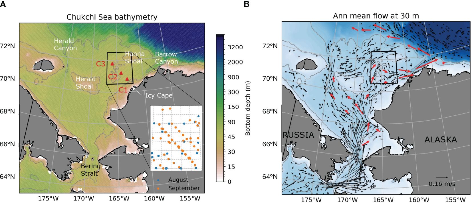
Figure 1 Map of the Chukchi Sea displaying bathymetry (A) and annual mean flow at 30 m (B), derived from the E3SM-Arctic-OSI simulation. (A) Thin gray contours denote isobaths at 40, 50, and 80 m. The red triangles represent the locations of the NOAA EcoFOCI Icy Cape moorings (C1–C3). The black box indicates the Icy Cape region, which is the focus area for mean calculations throughout this paper. The inset plot shows the locations of CTD casts conducted in August (blue dots) and September (orange dots) from 2010 to 2016 (see text for details). (B) Black vectors indicate simulated flow averaged over the period from 1987 to 2016. Red vectors indicate the mean Lagrangian velocity of drifters in each 1° latitude × 3° longitude box during ice-free seasons (Stabeno and McCabe, 2023).
We next focus on the Icy Cape region’s surface conditions by comparing sea surface temperature (SST) and sea ice concentration with the 1/4° monthly NOAA Optimum Interpolation SST (OISSTv2) reanalysis product (Reynolds et al., 2007) in Figure 2. The model adeptly reproduces monthly SST and sea ice concentration anomalies (with their mean annual cycles removed), showing a strong correlation with observed interannual variations (r = 0.83 for SST and r = 0.78 for sea ice concentration). However, the simulated variabilities in both SST and sea ice concentration are slightly more pronounced than observed, as suggested by the fitted regression lines having slopes less than 1 (Figures 2C, D).
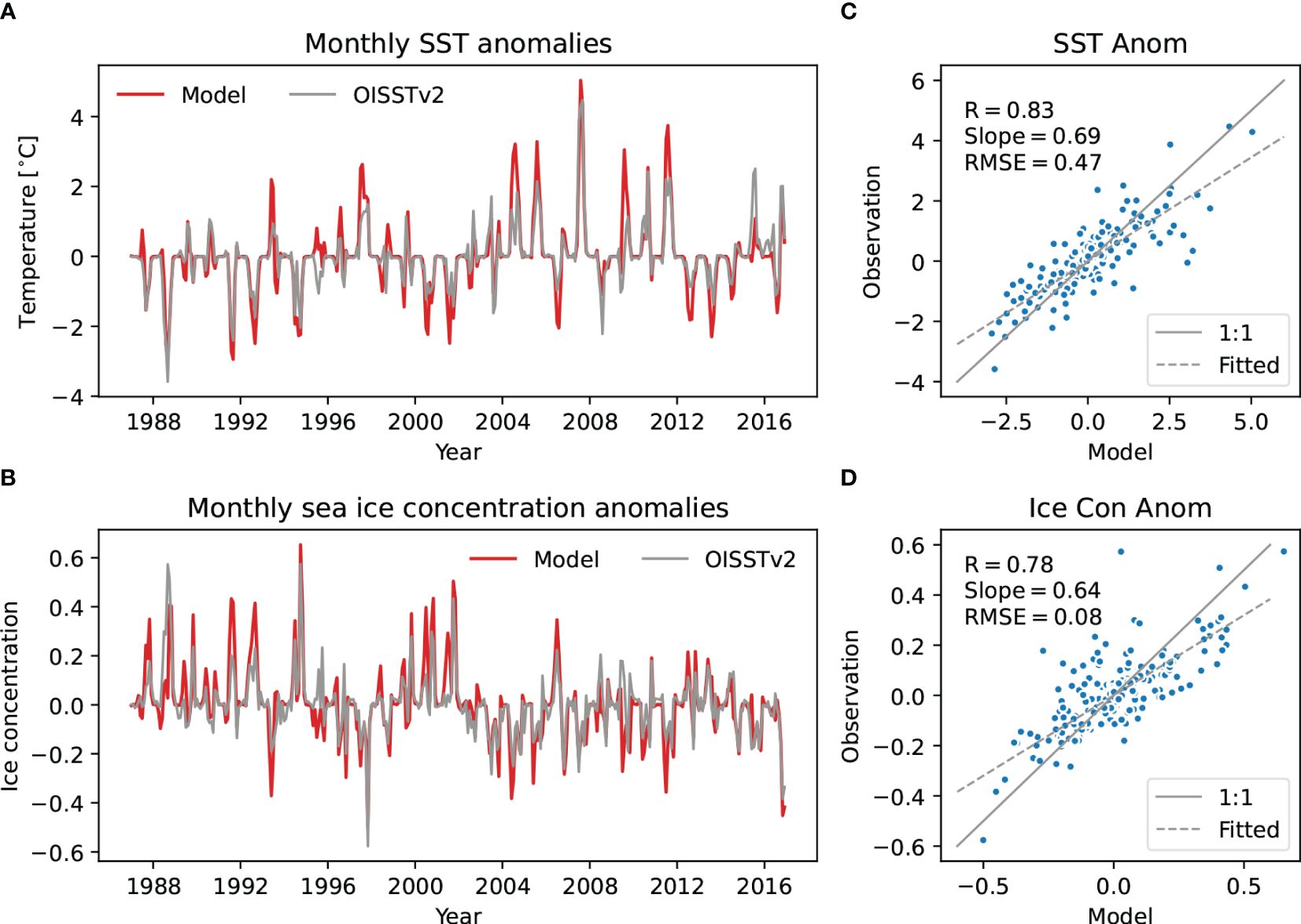
Figure 2 Comparison of monthly anomalies of sea surface temperature (SST; A and C) and sea-ice concentration (B, D) between the model and OISSTv2 reanalysis, averaged over the Icy Cape region. Anomalies are computed by removing individual climatological annual cycles from the monthly mean data. The left panels display time series, while the right panels depict point-to-point comparisons. In the right panels, the 1:1 line is depicted in solid gray, accompanied by statistical indicators including the correlation coefficient (R), fitted slope (shown by the dashed gray line), and root-mean-square error (RMSE).
We further compare the simulated near-bottom (46 m) temperature and salinity against data obtained from the NOAA EcoFOCI moorings along the Icy Cape section since 2010 (C1, C2, and C3, indicated by the red triangles in Figure 1A; Stabeno et al., 2018). Monthly anomalies are computed by removing the respective annual cycles of the period of 2010–2016. The model overall captures the observed interannual variability of the near-bottom temperatures (r = 0.74, p< 0.05), although it tends to slightly underestimate the variability at C1 (blue dots in Figure 3C). Additionally, summer peak temperatures at C1 is generally underestimated in the model, in agreement with Veneziani et al. (2022) where the model is found to underestimate the heat flux across Bering Strait with respect to observations. This coastal cold bias may stem from the model’s limited capability at the 10-km resolution to fully capture the warm ACC during summer, when the ACC can be very narrow and intense. But the model effectively replicates the interannual variability of the near-bottom salinity (r = 0.76, p< 0.05) (Figures 3B, D), indicating its ability to represent sea ice formation/brine rejection and retreat processes.
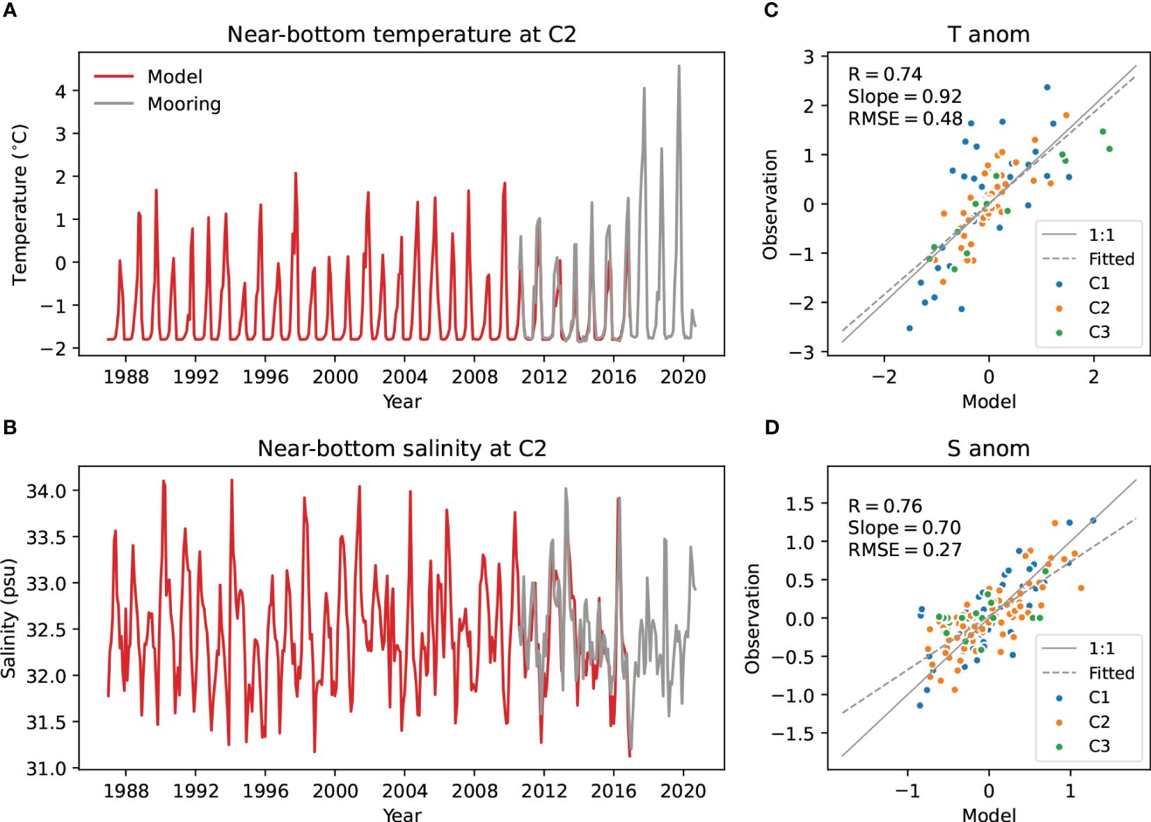
Figure 3 Comparison of monthly-mean near-bottom (46 m) temperature and salinity at the Icy Cape mooring locations, as indicated by triangles in Figure 1A. (A, B) Time series of C2, showcasing the best observational coverage. (C, D) A comparison of all available observational data from the three sites with corresponding model output spanning from 2010 to 2016. Monthly temperature and salinity anomalies are computed by removing the respective annual cycles of the 2010–2016 period.
To gain insight into the seasonal variations in stratification in the NE Chukchi Sea, we examine the monthly climatological vertical profiles of temperature, salinity, and buoyancy frequency in the Icy Cape region (Figure 4). The buoyancy frequency, defined as
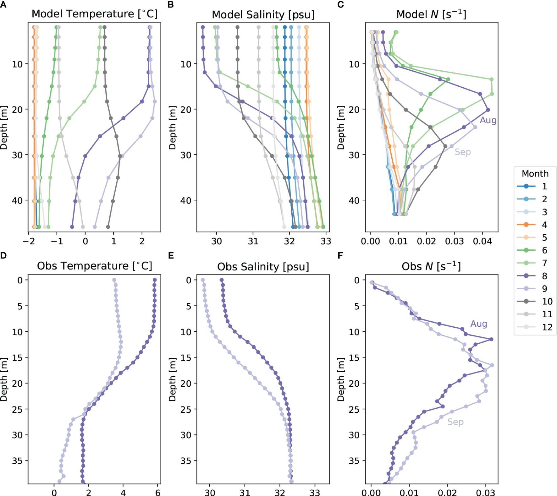
Figure 4 (A–C) Simulated climatological (1987–2016) profiles of temperature (A), salinity (B), and buoyancy frequency (C) averaged over the Icy Cape region. In temperature and salinity profiles, the markers along the lines indicate the depth corresponding to the bottom of grid cells, while for buoyancy frequency, the markers represent the grid centers used in calculations. (D, E) Averaged August and September profiles of temperature (D), salinity (E), and buoyancy frequency (F) derived from CTD casts conducted in this region between 2010 to 2016, with locations shown in Figure 1A. A compilation of 162 profiles has been employed to create these averages.
, where ρ is the potential density of seawater, is the reference seawater density of 1026 kg m−3 as used in the model, and ɡ is the gravitational acceleration, serves as our key metric for quantifying stratification.
Our analysis begins with examining seasonal changes from the model (Figure 4). The cold and frozen season in the NE Chukchi Sea shelf, extending from December to May, is characterized by temperatures near the freezing point of seawater and a well-mixed water column. Salinity gradually increases by about 1.3 psu during this period, indicative of the continuous formation of sea ice and brine rejection. Buoyancy frequency remains close to zero, reflecting the well-mixed nature of the water column. Starting in June, as sea ice melts and solar radiation intensifies, the upper layer warms and freshens more rapidly than the lower layer, leading to the formation of a two-layer structure. The upper layer reaches its maximum temperature and minimum salinity in August, after which it gradually undergoes cooling and salinification. Meanwhile, the lower layer continues to warm and freshen until October. Following these changes, the buoyancy frequency attains its maximum subsurface peak in July, which subsequently decreases while deepening over time. Starting in October, the water column undergoes cooling and salinification with thorough vertical mixing, eventually returning to its winter state.
We validate the model’s buoyancy profiles using available Conductivity, Temperature, and Depth (CTD) casts from the Icy Cape region, with 162 casts conducted between 2010 and 2016 and provided by NOAA’s EcoFOCI program (Mordy et al., 2023). Since these CTD observations predominantly cover the late summer, our comparison focuses on August and September profiles (see Figure 1A for locations). Although the CTD profiles are not evenly distributed temporally and spatially, with more frequent sampling nearshore than offshore, the observed maximum buoyancy frequency, where the pycnocline is defined, is generally centered around 15–20 meters in August and shifts deeper to 20–25 meters in September, aligning approximately with the model’s results (Figure 4F). This agreement in the vertical structure of stratification suggests that the model captures the basic characteristics of seasonal transitions in stratification. Therefore, we use it to further study the seasonal and interannual variability of these dynamics. We refer to the period from June to November, characterized by the two-layer structure, as the “summer” period and focus on this season for the rest of the paper.
We subsequently examine the interannual variability of the summer stratification and its associated hydrographic characteristics. We determine the annual maximum buoyancy frequency (Nmax) by first identifying the subsurface peak of N for individual months and then averaging these values over the summer season for each year. A higher value of Nmax indicates stronger stratification. We also calculate the depths at which Nmax occurs, namely the pycnocline depth, in a similar fashion. Figure 5 presents the time series of Nmax (red curve with an inverted y-axis) and the pycnocline depth (blue curve). It also includes time series of summer mean temperatures and salinities at both the surface and near-bottom (40 m) depths.
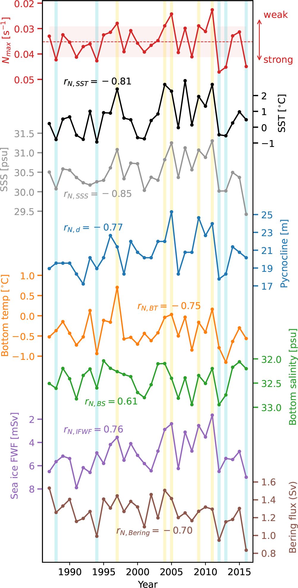
Figure 5 Time series showing simulated summer-mean stability and corresponding hydrographic properties in the Icy Cape region from 1987 to 2016. From top to bottom, the series includes maximum buoyancy frequency of the water column (Nmax); sea surface temperature; sea surface salinity; depth of the pycnocline; near-bottom temperature at 40 m; near-bottom salinity at 40 m; freshwater flux resulting from local sea ice melt; Bering Strait volume flux averaged from March to August. All summer-mean curves encompass the ice-free season from June to November except for the Bering Strait flux. Nmax is computed by first identifying the peak value of the water column for individual months and then averaging over the summer months for each year. The mean value of Nmax is represented by a dashed horizontal line, while the ±1σ range is indicated by the shaded band. These metrics have been used to define the years with weak versus strong stratification (as detailed in the text), which are highlighted by vertical yellow and blue shades, respectively. For ease of visual comparison, the y-axes of Nmax, near-bottom salinity, and sea-ice freshwater flux are inverted. Correlation coefficients between Nmax and individual curves are labeled. Vertical yellow shadings indicate weak stratification years, while vertical blue shadings indicate strong stratification years.
Notably, there is a negative correlation between the intensity of stratification Nmax and its depth (rN,D = −0.77, p< 0.05). Nmax is also negatively correlated with sea surface temperature and salinity (−0.81 and −0.85, respectively, both p< 0.05). In contrast, Nmax is negatively correlated with near-bottom temperature but positively correlated with near-bottom salinity (−0.75 and 0.61, respectively, both p< 0.05; note the inverted y-axis for bottom salinity). These results indicate that in the Icy Cape area, summers with weak stratification are associated with a warmer water column with a deeper pycnocline, featuring salty anomalies in the upper layer and fresh anomalies in the lower layer. Conversely, summers with strong stratification are characterized by colder temperatures across the water column and a shallower pycnocline, alongside fresh anomalies in the upper layer and salty anomalies in the lower layer.
The findings discussed previously might seem counterintuitive, as one would typically anticipate fresh upper-layer anomalies during warmer summers characterized by a greater influx of freshwater from melted ice and runoff (Woodgate et al., 2005). To further explore these hydrographic characteristics, we extend our analysis across the Chukchi Sea. We begin by reviewing climatological monthly maps of Chukchi Sea temperatures and salinities, superimposing the mean flow (see September as an example in Figure 6, and the entire summer in Supplementary Figure S2, S3). We find that, from June to November, the Chukchi Sea waters gradually warm from June to September, starting from the south and extending northward, followed by a cooling phase in October and November. This pattern of surface temperature evolution is closely aligned with the seasonal retreat and advance of sea ice (with a 15% concentration serving as the threshold for sea ice extent). A noteworthy aspect is the slight phase lag of about one month in water mass changes between the bottom and surface layers (Supplementary Figure S2).
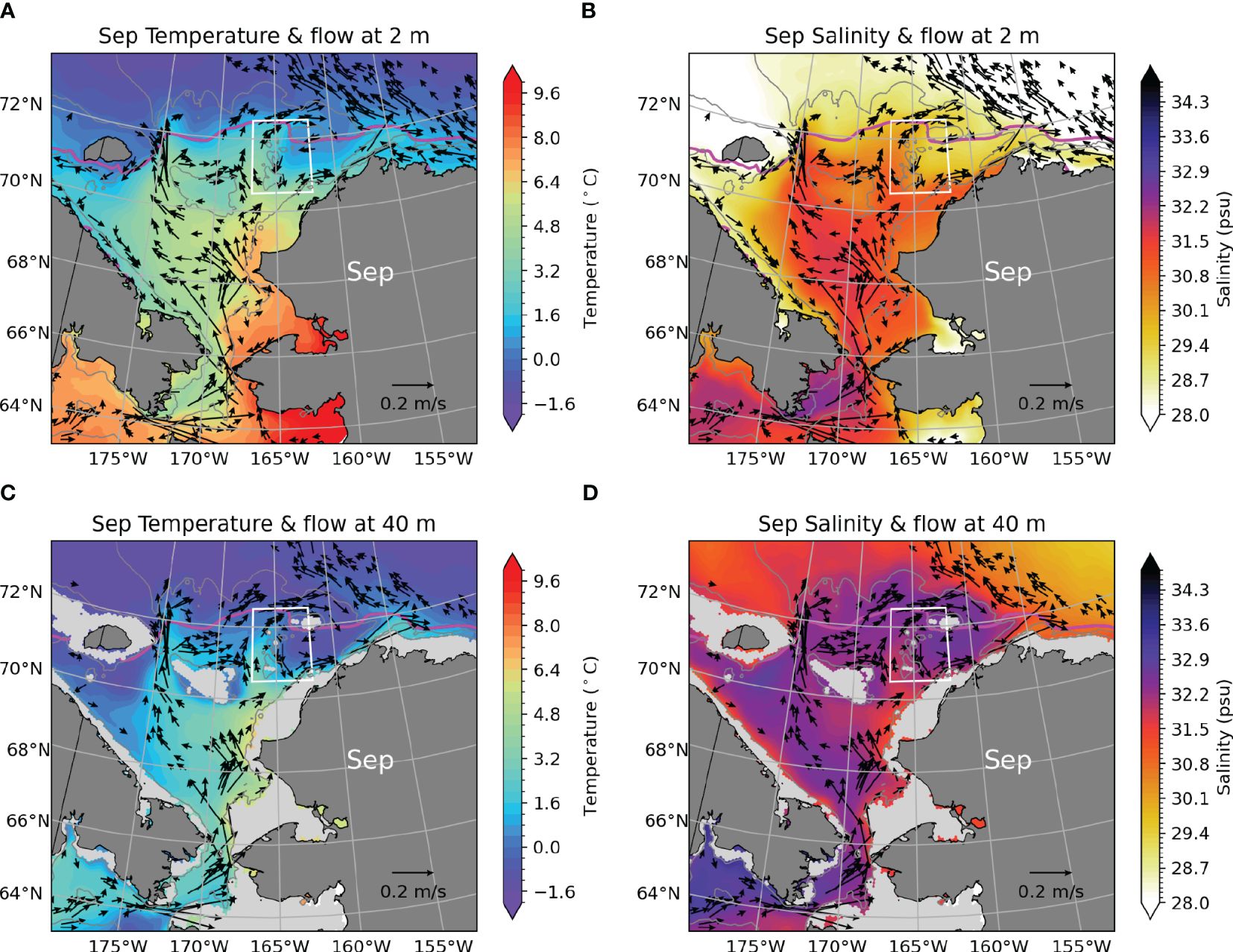
Figure 6 Climatological September temperature (left) and salinity (right) at near-surface (2 m; (A, B) and near-bottom (40 m; (C, D) depths. Vectors depict September mean flow at corresponding depths, subject to a minimum velocity threshold of 4 cm s−1. The white box in each subplot indicates the Icy Cape region.
However, the patterns of salinity are more intricate and intriguing (Supplementary Figure S3). Toward the end of winter (April–May), the entire shelf experiences thorough vertical mixing and its salinity reaches its annual maximum. Concurrently, the Bering Strait inflow and the waters along its pathways maintain relatively lower salinity, as ice formation is less active in the northern Bering Sea (except in polynias). As summer starts (June–July), the local melting of ice significantly freshens the upper layer across the shelf, while the lower layer preserves characteristics of cold, salty winter water. This process establishes a pronounced salinity gradient, creating a distinct two-layer structure. The Bering Strait inflow, with salinity levels intermediate between these two extremes, introduces relatively saline water to the upper layer and fresher water to the lower layer (Figures 6B, D), moderating the vertical salinity gradient along its path and consequently weakening stratification during summer. This finding is in line with the synthesized T-S diagram over the DBO5 section close to the head of Barrow Canyon in Pickart et al. (2019), their Figure 3), which illustrates that the salinity of Pacific-sourced water masses, including Alaskan Coastal Water and Bering Summer Water, is between those of the Melt Water and Winter Water masses.
To investigate the differences in hydrographic properties under weak and strong stratification conditions, we calculated the composite mean of upper layer temperature and salinity for years categorized by weak or strong summer stratification in the Icy Cape region. Weak stratification years are those where the maximum buoyancy frequency (Nmax) is more than one standard deviation (1σ) below its long-term mean (1987–2016) as shown in Figure 5 (specifically, years 1997, 2004, 2005, 2009, 2011 indicated by vertical yellow shading). Conversely, strong stratification is defined by Nmax exceeding the long-term mean by more than 1σ (namely, 1988, 1994, 2012, 2013, 2016 indicated by vertical blue shading).
Figures 7 and 8 display the deviations in composite mean sea surface temperature and salinity relative to their respective long-term averages. Results suggest that in conditions of weak stratification, there is a prevalent occurrence of warm and saline anomalies in the upper layer across the Chukchi shelf (Figure 7), despite Nmax being computed specifically for the NE Chukchi area. In contrast, strong stratification conditions are characterized by cooler and fresher anomalies (Figure 8). Interestingly, in both scenarios, the patterns of temperature and salinity anomalies exhibit a significant month-to-month consistency spanning across the Chukchi shelf towards the Arctic basin.
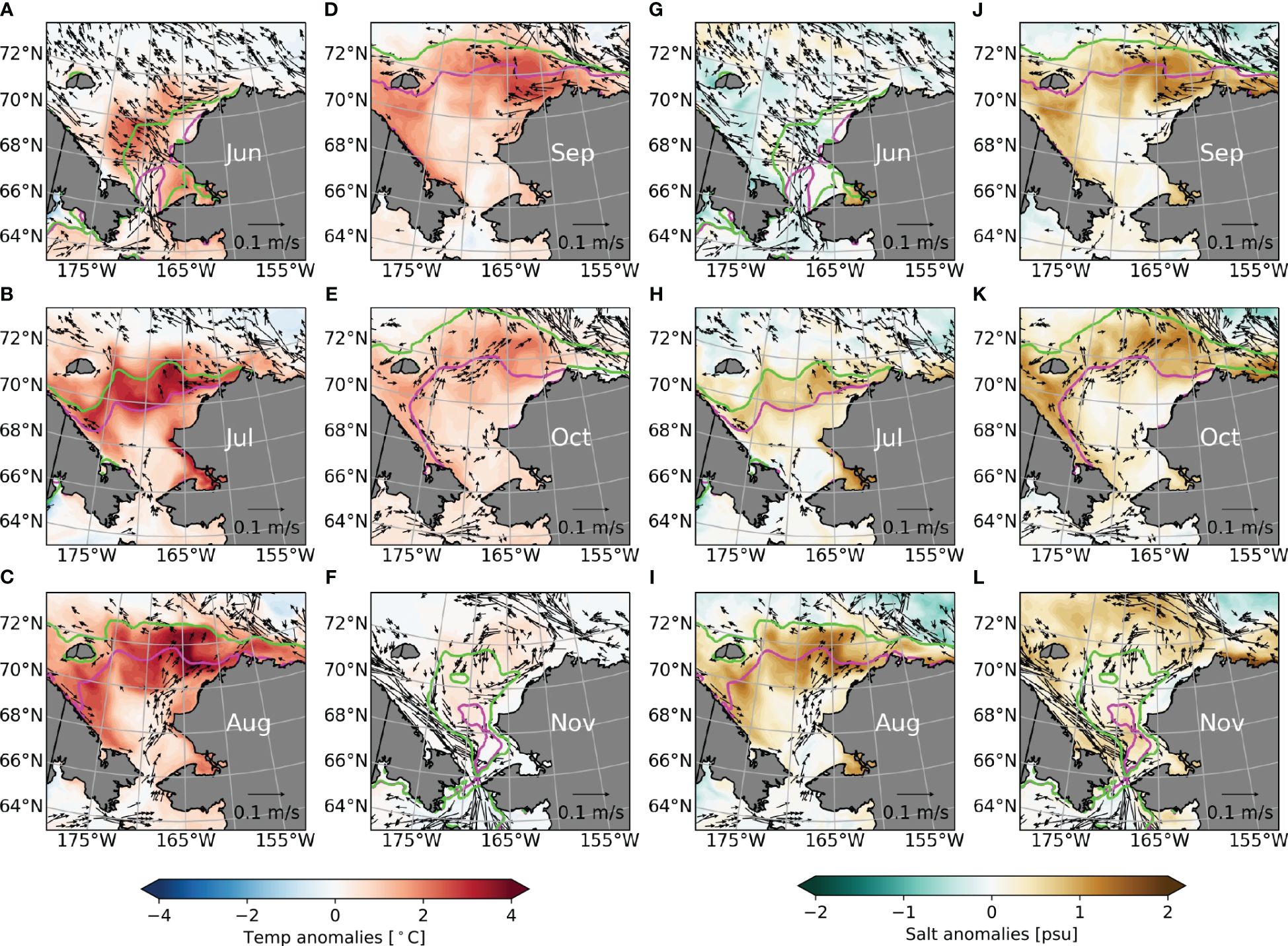
Figure 7 Composite map of sea surface anomalies in temperature (A–F) and salinity (G–L) during summers with weak stratification in the Chukchi Sea, relative to the 30-year climatology. Summers with weak stratification are defined as those instances when the buoyancy frequency Nmax is less than 1σ below the long-term mean based on Figure 5. For temperature and salinity values, refer to the colorbars located in the upper right and lower right, respectively. In each subplot, vectors indicate anomalous surface flow patterns, subject to a minimum threshold of 2 cm s−1. The magenta contour represents the average sea-ice extent (corresponding to 15% sea-ice concentration), while the green contour shows the sea-ice extent during summers with weak stratification.
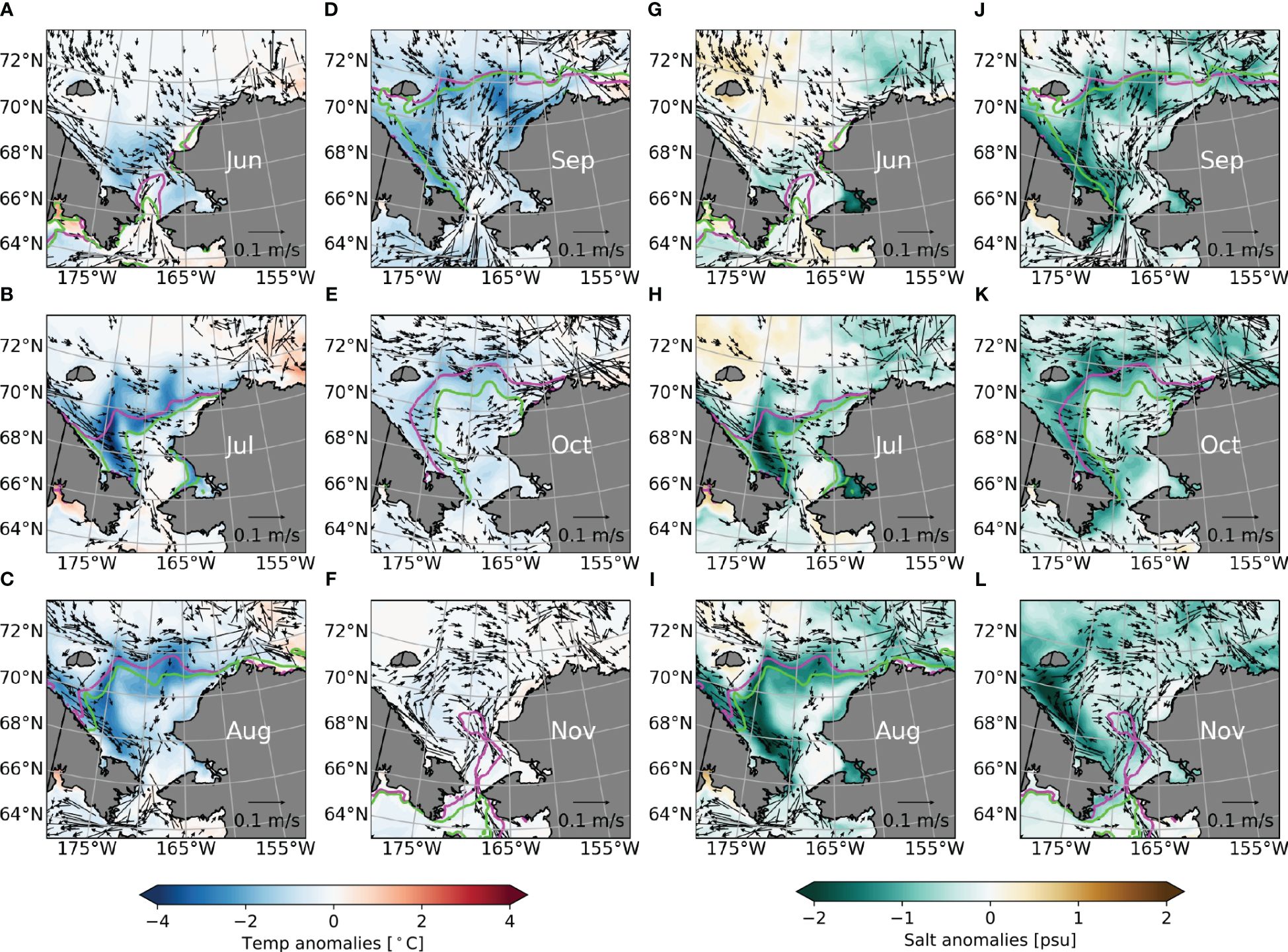
Figure 8 Same as Figure 7, but for summers with strong stratification. Summers with strong stratification are defined as those instances when the buoyancy frequency Nmax is greater than 1σ above the long-term mean based on Figure 5.
In the lower layer, the temperature and salinity anomalies are of smaller magnitudes compared to the upper layer, showing warm, fresh anomalies during weak stratification conditions and cold, saline anomalies during strong stratification conditions (Supplementary Figures S4, S5). These results align with the findings presented in Figure 5, where warmer summers are associated with a saltier upper layer and a fresher lower layer, while cooler summers correspond with a fresher upper layer and a saltier lower layer.
Next, we overlay sea-ice extent and anomalous ocean currents on the maps of temperature and salinity anomalies (Figures 7, 8). We notice that changes in sea-ice extent, as indicated by the band between the composite mean (green contour) and the climatological mean (magenta contour) in each subfigure, coincide with the strongest temperature and salinity anomalies. This consistency is most noticeable from July to October when the melting of sea ice is most significant. This alignment leads us to hypothesize that the timing of the sea ice retreat and associated meltwater flux could be an important factor that impacts changes in ocean stratification. Additionally, the intensity of the Bering Strait inflow varies between these two stratification scenarios. During periods of weak stratification, there is an enhanced influx from June to August, as evidenced by the anomalous northward surface flow vectors near the Bering Strait (Figure 7). In contrast, during strong stratification years, the northward transport around the Bering Strait is noticeably reduced (Figure 8). The roles of sea ice and Bering Strait inflow in these different scenarios will be explored in the next section.
In previous sections, we demonstrated a negative correlation between summer stratification in the NE Chukchi Sea and both SST and SSS (Section 3). Our findings indicate that periods of weak stratification are typically associated with unusually warm and saline conditions at the surface, while strong stratification corresponds with cooler and less saline conditions. Furthermore, we found that during weak stratification periods, the lower layer tends to exhibit warm and fresh characteristics, opposite to what happens during periods of strong stratification. Our investigations also uncover consistent, shelf-wide temperature and salinity anomaly patterns over time, including distinct sea-ice extent and flow patterns (Section 4). This section aims to explore the physical processes driving the seasonal and interannual variations in the stratification of the NE Chukchi Sea. We examine impact of the timing of sea-ice retreat and the resulting changes in freshwater flux, as well as changes in circulation and the associated transport of Pacific water.
We first investigate the dynamics of local sea ice and its direct impact on upper-layer salinity through meltwater contribution. Typically, sea-ice concentration and volume in the region starts to diminish in May and reaches its minimum in September (Supplementary Figure S7). In years characterized by weaker stratification, sea-ice concentration and volume decline faster, consistent with higher SSTs during these periods. This warmer ocean state would, on average, necessitate more time to reach the freezing point in the fall. In periods with weak stratification, the NE Chukchi Sea experiences a prolonged duration of ice concentrations below 20%, with up to three months ice-free conditions in August to October. By contrast, years of strong stratification exhibit a slower retreat and earlier formation of sea ice in the fall, leading to just one month with less than 20% ice concentration.
Despite the rapid decline of sea ice in the early summers of years with weak stratification, this phenomenon does not translate into an increased meltwater flux in the region. Rather, it causes a reduction in meltwater input, leading to a saltier upper layer. This is evidenced by the positive correlation between stratification strength and local sea-ice meltwater flux (purple curve in Figure 5; r = 0.76, p< 0.05) and elevated SSS (gray curve in Figure 5). This pattern implies that during years characterized by weak stratification, the early retreat of sea ice leads to a lack of ice available for melting during the peak warmth of July and August, likely due to the northward transport of sea ice prior to local melting. Conversely, in years marked by strong stratification, the delayed retreat of sea ice increases meltwater availability in the Icy Cape region, contributing to a fresher upper layer that amplifies the water column’s density gradient.
To investigate the variability of the Bering Strait inflow, we first compute its volume and freshwater flux and compare it to observational estimates derived from year-round moorings located at the Bering Strait (Woodgate and Peralta-Ferriz, 2021; Supplementary Figure S6). The simulation produces a long-term mean Bering Strait volume influx of 0.99 Sv (1 Sv ≡ 106 m3/s), closely aligning with observational estimates (0.97 ± 0.12 Sv). The mean freshwater flux is 75 mSv, within the observed range of 63–95 mSv (the higher estimate accounts for corrections for the ACC and surface layer/stratification). The model also shows notable consistency with observed interannual variability. However, it does not replicate the recently observed positive trend, a limitation also reported in other modeling studies (Clement Kinney et al., 2014).
Furthermore, we calculate a six-month running mean of the monthly Bering Strait volume flux for each year from 1987 to 2016, creating a time series of 30 points. This calculation is repeated six times, each time shifting the six-month window by one month, thereby producing six distinct time series. These series are correlated with the summer Nmax presented previously. The most pronounced correlation is found when the Bering influx precedes the summer Nmax by three months (the brown curve in Figure 5), yielding a correlation coefficient of r = −0.70 (p< 0.05). The three-month delay between the Bering Strait transport and its influence on the stratification at Icy Cape aligns with both observations (Stabeno et al., 2018) and prior modeling studies (Spall, 2007). Such a negative correlation is consistent with the composite results in Section 4, where years with weak stratification are associated with a robust Bering Strait inflow in early summer (Figure 7), and the opposite is true for years with strong stratification (Figure 8).
Up to this point, we have found that interannual fluctuations in sea-ice meltwater flux and Bering Strait flux are closely linked to variations in stratification at the Icy Cape. To further assess their respective contributions to stratification, we have calculated the heat and freshwater fluxes within the Icy Cape domain. The surface heat flux comprises the combined effects of shortwave, longwave, latent, and sensible heat fluxes, along with the heat flux resulting from sea-ice melting. Similarly, the surface freshwater flux is diagnosed as the sum of evaporation, precipitation, runoff, meltwater from sea ice, and the flux required to restore SSS to observed values. The lateral heat and freshwater fluxes are diagnosed as
and
respectively. Here, v represents the normal velocity, including both the mean flow and bolus velocity to account for eddy effects, T and S are temperature and salinity, is the reference salinity of 34.8 psu (Aagaard and Carmack, 1989; Woodgate et al., 2005), and H is the depth of the water column. All diagnoses are based on monthly outputs from the model.
The climatological annual cycle of heat flux in the Icy Cape region reveals a net heat gain from May to September, with a loss during the remaining months (solid curve in Figure 9A). Decomposition shows that this heat gain stems from both surface and lateral inputs, while heat loss primarily occurs through surface processes in the fall (solid curves in Figure 9C). Further analysis of the surface heat flux reveals that incoming shortwave radiation drives the slight heat gain in summer, while sensible, latent, and longwave radiation, along with heat used for sea-ice melting, contribute to significant heat loss in the fall (Figure 9E). In years with weak stratification, the system gains approximately 7.6 EJ (1 EJ ≡ 1018 Joules) more heat compared to the climatological mean (heat flux integration from May to September). About 60% of this increase is attributed to surface fluxes and 40% to lateral heat transport. This enhanced heat gain corresponds with higher summer temperatures at both surface and near-bottom levels (Figure 5). Conversely, during years with strong stratification, the system gains 10.7 EJ less heat than climatology, mostly due to diminished lateral heat transport. This results in cooling throughout the water column (Figure 5).
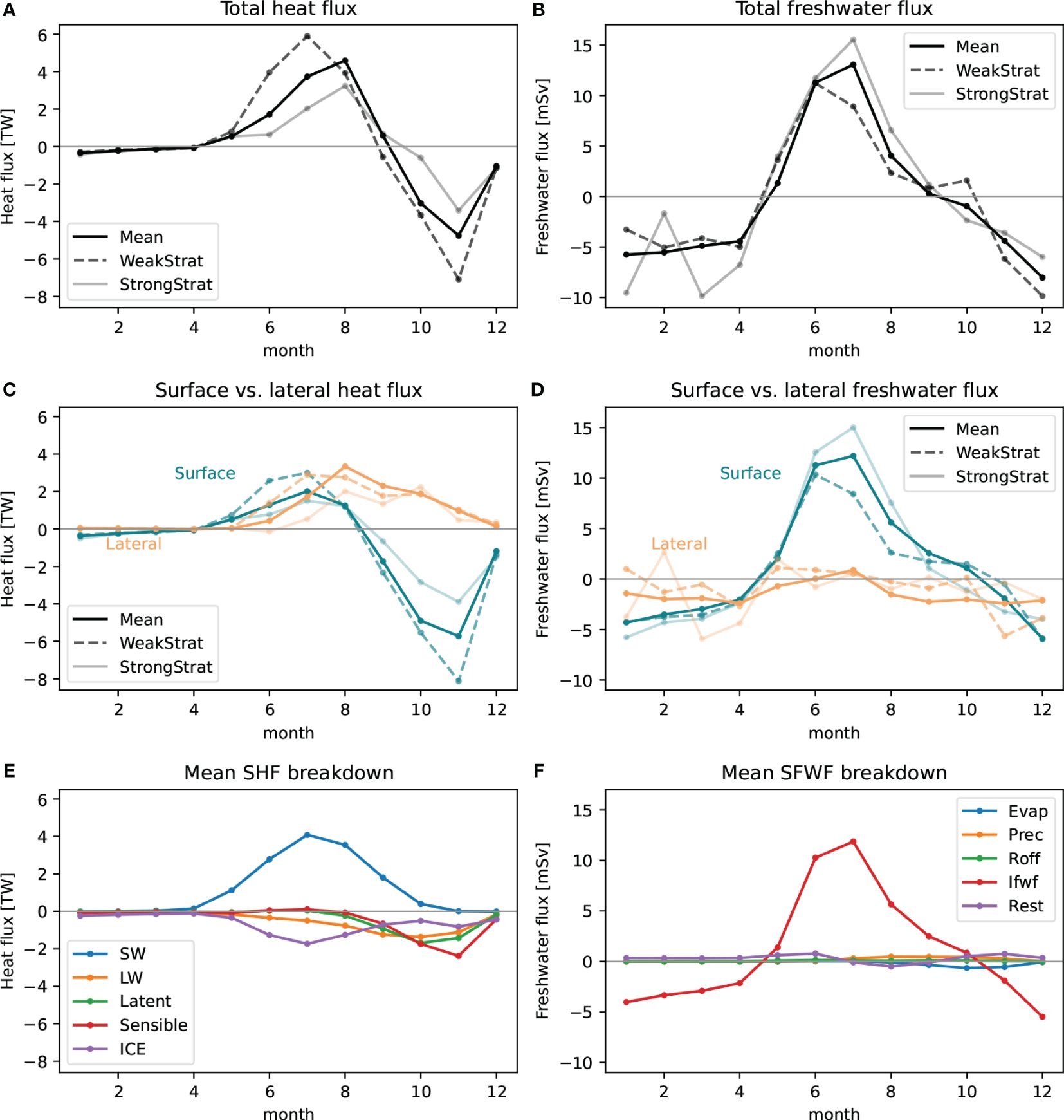
Figure 9 Annual cycles of heat and freshwater fluxes. (A, B) Total heat and freshwater flux of climatological mean (dark solid), years of weak stratification (dashed), and years of strong stratification (light solid). (C, D) Breakdown of the total heat and freshwater fluxes into their surface and lateral components. (E) Further breakdown of the surface heat flux into shortwave, longwave, latent, and sensible heat flux, as well as heat flux attributable to sea ice melting. (F) Further breakdown of the surface freshwater flux into contributions from evaporation, precipitation, river runoff, sea-ice freshwater flux, and the effect of restoring of surface salinity to observational values.
Regarding the climatological annual cycle of freshwater flux, the domain generally gains freshwater from May to September and loses it for the remainder of the year (solid curve in Figure 9B). This seasonal cycle is predominantly driven by surface flux, while lateral flux tends to lose freshwater (gain salt) and exhibits a milder seasonal variation (solid curves in Figure 9D). The primary contributor to the surface freshwater flux is sea-ice meltwater (Figure 9F).
During weak stratification years, the system experiences a reduction in total freshwater transport by 8.3 km3 from May to September relative to the climatological mean, with a 21.3 km3 decrease from surface transport partly offset by a 13.1 km3 increase in lateral transport. This decrease in total freshwater transport leads to higher salinity in the upper layer (evidenced by higher SSS in Figure 5). As the density gradient is more influenced by salinity than temperature in this region, this increase in upper-layer salinity results in a reduced vertical density gradient, hence weaker stratification. In contrast, strong stratification years see a 23.9 km3 increase in freshwater gain, with 12.1 km3 from surface flux and 11.8 km3 from lateral flux. This additional freshwater enhances the vertical density gradient, leading to stronger stratification.
Although it contributes little to the seasonal cycle of surface freshwater flux (Figure 9F), the surface restoring term affects its interannual variability. Sea-ice meltwater is the dominant factor in surface freshwater flux, but its variability is reduced by approximately 25% due to the restoring term (Supplementary Figure S8). This suggests that while the freshening effect from excess sea-ice meltwater during strong-stratification summers is somewhat mitigated by surface restoring, it remains the primary cause of strong stratification, and vice versa for weak-stratification summers.
In summary, our flux calculation suggests that the timing of sea-ice retreat and the consequent variations in meltwater flux are the primary factors driving interannual changes in stratification in the Icy Cape region. These findings highlight the predominance of meltwater flux in influencing stratification, overwhelming the effects of changes in circulation and associated lateral freshwater transport.
A natural follow-up question is: What factors drive the systematic changes in the timing of sea-ice retreat and Bering Strait inflow? In other words, why does an early sea-ice retreat typically coincide with enhanced Bering Strait inflow, and vice versa? To address this question, we next examine the surface winds over the Bering and Chukchi seas, which are notably influenced by the strengths and positions of the Siberian High, Beaufort High, and Aleutian Low pressure systems (Overland and Wang, 2010). From November through May, this region typically experiences strong south-to-southwestward winds, which are driven by a robust pressure gradient (Figure 10A). The Aleutian Low shifts westward from the Gulf of Alaska in November to the Aleutian Basin in December and subsequently intensifies (Supplementary Figure S9).

Figure 10 Sea level pressure (SLP) and 10-m wind patterns in the northern Bering and Chukchi seas, derived from the JRA55-do v1.3 dataset that was used to drive the model. (A) The climatological SLP and wind patterns for winter (November to May). (B) Composite map showing the anomalous SLP and wind patterns during winters of years with weak stratification, as defined in Section 4. (C) Similar to (B), but for years with strong stratification.
In years characterized by weak stratification in the NE Chukchi Sea, an underdeveloped Aleutian Low is observed in November, with a delayed westward shift until January (Supplementary Figure S9). This results in a significantly reduced pressure gradient and anomalous north-to-northeastward winds (Figure 10B), which advect warmer air from the south and facilitate a faster northward retreat of sea ice in spring and simultaneously promote a stronger northward flow through the Bering Strait. Conversely, during years with strong stratification, the Aleutian Low remains abnormally strong throughout the winter (Supplementary Figure S9), leading to more intense south-to-southwestward winds (Figure 10C) that advect cold air from the north and delay sea-ice retreat in spring and meanwhile hinder the northward Bering Strait transport. These findings align with previous research suggesting that the annual transport through Bering Strait is primarily set by the longitudinal displacement of the Aleutian Low and the associated changes in wind stress (Danielson et al., 2014).
To better understand the seasonal and interannual variability in stratification within the NE Chukchi Sea, an area crucial for supporting a rich marine ecosystem, we conducted an analysis using a hindcast simulation from a global ocean-sea ice model forced by JRA55-do. This model, featuring a refined 10 km resolution in the Arctic region and a 60 km resolution for the rest of the globe, covered the period from 1958 to 2016, and its last 30 years were used in our study. Our analysis, which included a comparison with available observations, focused on the Icy Cape region of the NE Chukchi Sea.
In our simulation, the NE Chukchi Sea exhibits pronounced seasonal hydrographic shifts, transitioning from a well-mixed state in winter (December to May) to a stratified two-layer structure in the warmer months (June to November), with peak stratification typically occurring in July. We found substantial interannual variability in stratification strength, which shows a strong negative correlation with both surface temperatures and salinities. During summers with weak stratification, the water column is generally warmer, featuring a saltier upper layer and a fresher lower layer, leading to a diminished vertical density gradient. In contrast, during summers with strong stratification, the water column is cooler, marked by a fresher upper layer and a saltier lower layer, resulting in a more pronounced density gradient.
Upon extending our analysis across the entire Chukchi shelf, we found that temperature and salinity anomalies exhibit significant consistency month-to-month, highlighting their links to both sea ice retreat and the intensity of Bering Strait inflow. Further quantification of heat and freshwater fluxes identified key factors influencing these variations. Notably, the interannual shifts in summer stratification within the NE Chukchi Sea are primarily driven by the timing of sea ice retreat and subsequent changes in meltwater flux. Specifically, an earlier retreat of sea ice leads to diminished meltwater influx during summer, engendering a saltier upper layer and consequently weaker stratification. This effect is more pronounced than any resulting from alterations in circulation (including an enhanced Bering Strait inflow) and the associated lateral freshwater transport. Furthermore, we found a concurrence between earlier sea ice retreat in the NE Chukchi and enhanced Bering Strait transport, and vice versa. This synchronized behavior is associated with the strength and location of the Aleutian Low pressure system, and timing of its westward shift from the Gulf of Alaska to the Aleutian Basin in early winter. The key findings have been summarized in Figure 11.
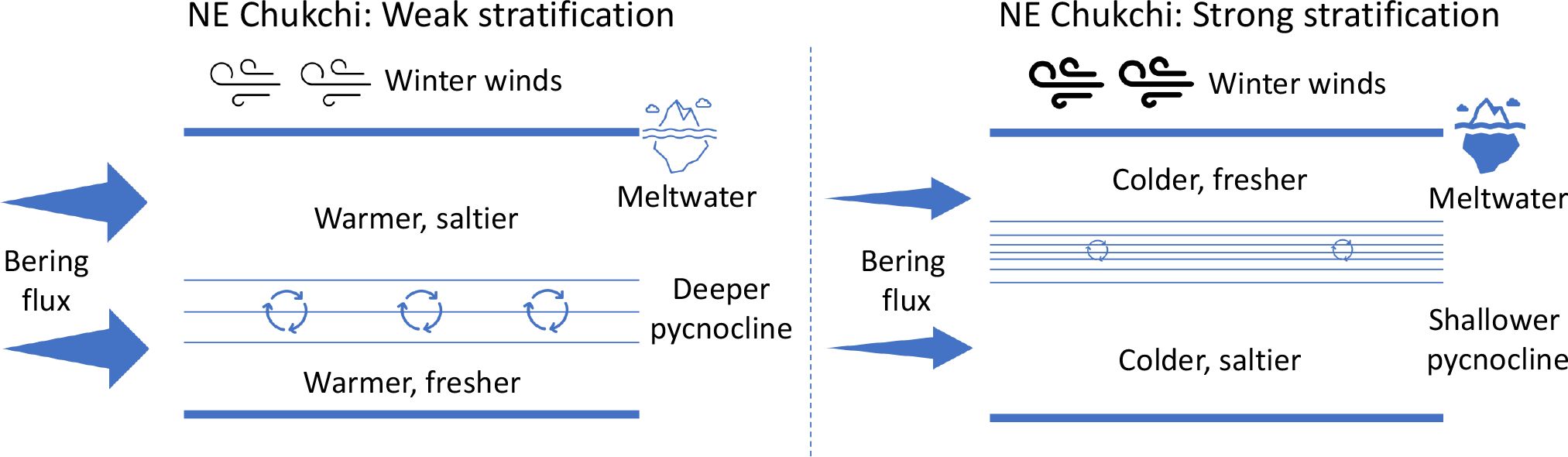
Figure 11 Schematic plot summarizing the hydrographic differences between weak and strong stratification summers in the NE Chukchi Sea and the associated controlling processes. During weak stratification summers, the water column is warmer with a saltier upper layer and a fresher lower layer, resulting in a diminished vertical density gradient. The opposite is observed during strong stratification summers. These differences are primarily driven by the timing of sea ice retreat and subsequent meltwater flux changes. An earlier sea ice retreat reduces meltwater influx, leading to a saltier upper layer and weaker stratification. This effect outweighs changes in circulation, including Bering Strait inflow. Additionally, the synchronization of early sea ice retreat and enhanced Bering Strait transport is linked to the strength and timing of the Aleutian Low’s westward shift from the Gulf of Alaska to the Aleutian Basin in early winter.
This study’s findings have profound implications for marine biology and ecosystems in the NE Chukchi Sea. On one hand, weak stratification promotes robust vertical mixing, which, during summers of weak stratification, enhances the upward transport of nutrients. Given that primary production in the Chukchi Sea is largely nutrient-driven, an increase in nutrient supplies could significantly bolster primary production. This correlation has been underscored by observational studies that link primary production in the Chukchi Sea directly to freshwater content variability (Yun et al., 2016). Moreover, weak stratification facilitates the influx of nutrient-rich Pacific water into the region, further enhancing the nutrient availability essential for primary production. On the other hand, our research also suggests that weak stratification corresponds with a deeper mixed layer and pycnocline, which could restrict light availability. Considering that various phytoplankton taxonomic groups (such as diatoms, cyanobacteria, cryptophytes) exhibit distinct responses to shifts in light availability, nutrients, and ambient temperatures (Finkel et al., 2016; Kremer et al., 2017), the interplay of weak stratification and a deeper mixed layer might favor certain phytoplankton groups (e.g., larger-sized phytoplankton) to thrive and possibly sustain a subsurface bloom beyond the spring bloom.
Our study underscores the controlling role of sea-ice retreat timing and its associated meltwater flux in dictating ocean stratification in the NE Chukchi Sea. Therefore, the timing of sea-ice retreat emerges as a valuable indicator for forecasting changes in summer stratification over seasonal time scales. However, future projections of stratification patterns in this region under climate change scenarios present a complex challenge. As the climate continues to warm, especially under the most aggressive greenhouse gas emission scenarios, we anticipate an earlier retreat of sea ice (Stroeve et al., 2007), a phenomenon likely to lead to relatively weak summer stratification. However, complicating this outlook is the expected intensification of the Aleutian Low under such warming conditions (Gan et al., 2017). An intensified Aleutian Low could delay sea-ice retreat and reduce Bering Strait inflow, as shown in our study, potentially resulting in stronger summer stratification in the region. These complexities highlight the need for continued research to refine our understanding and predictions of stratification dynamics in the rapidly changing Arctic environment.
The version of the E3SMv1 model used to run E3SM-Arctic-OSI is available on Zenodo (https://doi.org/10.5281/zenodo.5548434). The model data used for the analysis presented in this paper are also available through Zenodo (https://doi.org/10.5281/zenodo.5548528). The sea surface temperature and sea ice data of OISSTv2 reanalysis can be accessed through https://psl.noaa.gov/data/gridded/data.noaa.oisst.v2.highres.html. The NOAA EcoFOCI drifter and mooring data will be made available on request. The CTD casts, 2012–2019 over the Icy Cape region can be accessed through the following list: https://doi.org/10.25921/3fs3-5e91; https://doi.org/10.25921/fcag-rk21; https://doi.org/10.25921/zahv-5m85; https://doi.org/10.25921/3wq6-0k19; https://doi.org/10.25921/jcvz-0s37; https://doi.org/10.25921/eqva-az08; https://doi.org/10.25921/n4yv-xs68; https://doi.org/10.25921/bs4a-4a30; https://doi.org/10.25921/hyqy-hn70; https://doi.org/10.7284/907640; https://doi.org/10.18739/A22B8VC6F; https://doi.org/10.25921/3jk6-ds75. Older CTD data 2010–2012 can be accessed at NOAA NCEI, Accession Numbers 155761, 169502, and 169625.
JZ: Conceptualization, Data curation, Formal analysis, Investigation, Methodology, Visualization, Writing – original draft, Writing – review & editing. WC: Conceptualization, Funding acquisition, Investigation, Project administration, Resources, Supervision, Writing – original draft, Writing – review & editing. PS: Conceptualization, Data curation, Investigation, Methodology, Resources, Supervision, Writing – original draft, Writing – review & editing. MV: Formal analysis, Methodology, Software, Validation, Writing – original draft, Writing – review & editing. WW: Methodology, Resources, Supervision, Writing – original draft, Writing – review & editing. RM: Data curation, Methodology, Validation, Writing – original draft, Writing – review & editing.
The author(s) declare financial support was received for the research, authorship, and/or publication of this article. This publication was partially funded by the Cooperative Institute for Climate, Ocean, & Ecosystem Studies (CICOES) under NOAA Cooperative Agreement NA20OAR4320271, through CICOES’s Research Development Grants. This research was also supported by the Regional and Global Model Analysis (RGMA) component of the Earth and Environmental System Modeling (EESM) program of the U.S. Department of Energy’s Office of Science, as a contribution to the HiLAT-RASM project.
The authors thank Shaun Bell and Peggy Sullivan for their assistance in acquiring the NOAA EcoFOCI mooring data and the CTD data in the Icy Cape region. This is CICOES Contribution #2024–1361, NOAA PMEL Contribution #5575, EcoFOCI Contribution #1050.
The authors declare that the research was conducted in the absence of any commercial or financial relationships that could be construed as a potential conflict of interest.
All claims expressed in this article are solely those of the authors and do not necessarily represent those of their affiliated organizations, or those of the publisher, the editors and the reviewers. Any product that may be evaluated in this article, or claim that may be made by its manufacturer, is not guaranteed or endorsed by the publisher.
The Supplementary Material for this article can be found online at: https://www.frontiersin.org/articles/10.3389/fmars.2024.1415021/full#supplementary-material
Aagaard K., Carmack E. C. (1989). The role of sea ice and other fresh water in the Arctic circulation. J. Geophysical Research: Oceans 94, 14485–14498. doi: 10.1029/JC094iC10p14485
Aagaard K., Roach A. (1990). Arctic ocean-shelf exchange: Measurements in Barrow Canyon. J. Geophysical Research: Oceans 95, 18163–18175. doi: 10.1029/JC095iC10p18163
Arrigo K. R., Perovich D. K., Pickart R. S., Brown Z. W., van Dijken G. L., Lowry K. E., et al. (2014). Phytoplankton blooms beneath the sea ice in the Chukchi Sea. Deep Sea Res. Part II: Topical Stud. Oceanography 105, 1–16. doi: 10.1016/j.dsr2.2014.03.018
Bates N. R. (2006). Air-sea CO2 fluxes and the continental shelf pump of carbon in the Chukchi Sea adjacent to the Arctic Ocean. J. Geophysical Research: Oceans 111, C10013. doi: 10.1029/2005JC003083
Clement Kinney J., Maslowski W., Aksenov Y., de Cuevas B., Jakacki J., Nguyen A., et al. (2014). On the flow through Bering Strait: A synthesis of model results and observations. In: Grebmeier, J., Maslowski, W. (eds) The Pacific Arctic Region. Springer, Dordrecht. 167–198. doi: 10.1007/978-94-017-8863-2_7
Danielson S. L., Ahkinga O., Ashjian C., Basyuk E., Cooper L., Eisner L., et al. (2020). Manifestation and consequences of warming and altered heat fluxes over the Bering and Chukchi Sea continental shelves. Deep Sea Res. Part II: Topical Stud. Oceanography 177, 104781. doi: 10.1016/j.dsr2.2020.104781
Danielson S. L., Weingartner T. J., Hedstrom K. S., Aagaard K., Woodgate R., Curchitser E., et al. (2014). Coupled wind-forced controls of the Bering–Chukchi shelf circulation and the Bering Strait throughflow: Ekman transport, continental shelf waves, and variations of the Pacific–Arctic sea surface height gradient. Prog. Oceanography 125, 40–61. doi: 10.1016/j.pocean.2014.04.006
Finkel Z., Follows M., Irwin A. (2016). Size-scaling of macromolecules and chemical energy content in the eukaryotic microalgae. J. Plankton Res. 38, 1151–1162. doi: 10.1093/plankt/fbw057
Gan B., Wu L., Jia F., Li S., Cai W., Nakamura H., et al. (2017). On the response of the Aleutian low to greenhouse warming. J. Climate 30, 3907–3925. doi: 10.1175/JCLI-D-15-0789.1
Gent P. R., McWilliams J. C. (1990). Isopycnal mixing in ocean circulation models. J. Phys. Oceanography 20, 150–155. doi: 10.1175/1520-0485(1990)020<0150:IMIOCM>2.0.CO;2
Kremer C. T., Thomas M. K., Litchman E. (2017). Temperature-and size-scaling of phytoplankton population growth rates: Reconciling the Eppley curve and the metabolic theory of ecology. Limnology oceanography 62, 1658–1670. doi: 10.1002/lno.10523
Ladd C., Mordy C., Salo S., Stabeno P. (2016). Winter water properties and the Chukchi Polynya. J. Geophysical Research: Oceans 121, 5516–5534. doi: 10.1002/2016JC011918
Large W. G., McWilliams J. C., Doney S. C. (1994). Oceanic vertical mixing: A review and a model with a nonlocal boundary layer parameterization. Rev. geophysics 32, 363–403. doi: 10.1029/94RG01872
Lewis K., Van Dijken G., Arrigo K. R. (2020). Changes in phytoplankton concentration now drive increased Arctic Ocean primary production. Science 369, 198–202. doi: 10.1126/science.aay8380
Li S., Lin P., Dou T., Xiao C., Itoh M., Kikuchi T., et al. (2022). Upwelling of atlantic water in barrow canyon, chukchi sea. J. Geophysical Research: Oceans 127, e2021JC017839. doi: 10.1029/2021JC017839
Lin P., Pickart R. S., McRaven L. T., Arrigo K. R., Bahr F., Lowry K. E., et al. (2019). Water mass evolution and circulation of the northeastern Chukchi Sea in summer: Implications for nutrient distributions. J. Geophysical Research: Oceans 124, 4416–4432. doi: 10.1029/2019JC015185
Lin P., Pickart R. S., Våge K., Li J. (2021). Fate of warm Pacific water in the Arctic basin. Geophysical Res. Lett. 48, e2021GL094693. doi: 10.1029/2021GL094693
Lowry K. E., van Dijken G. L., Arrigo K. R. (2014). Evidence of under-ice phytoplankton blooms in the Chukchi Sea from 1998 to 2012. Deep Sea Res. Part II: Topical Stud. Oceanography 105, 105–117. doi: 10.1016/j.dsr2.2014.03.013
Lu K., Danielson S., Weingartner T. (2022). Impacts of short-term wind events on Chukchi hydrography and sea-ice retreat. Deep Sea Res. Part II: Topical Stud. Oceanography 199, 105078. doi: 10.1016/j.dsr2.2022.105078
MacKinnon J. A., Simmons H. L., Hargrove J., Thomson J., Peacock T., Alford M. H., et al. (2021). A warm jet in a cold ocean. Nat. Commun. 12, 2418. doi: 10.1038/s41467-021-22505-5
Mordy C. W., Bond N. A., Cokelet E. D., Deary A., Lemagie E., Proctor P., et al. (2023). Progress of fisheries-oceanography coordinated investigations in the Gulf of Alaska and Aleutian Passes. Oceanography 36, 94–100. doi: 10.5670/oceanog
Nummelin A., Ilicak M., Li C., Smedsrud L. H. (2016). Consequences of future increased Arctic runoff on Arctic Ocean stratification, circulation, and sea ice cover. J. Geophysical Research: Oceans 121, 617–637. doi: 10.1002/2015JC011156
Okkonen S., Ashjian C., Campbell R. G., Alatalo P. (2019). The encoding of wind forcing into the Pacific-Arctic pressure head, Chukchi Sea ice retreat and late-summer Barrow Canyon water masses. Deep Sea Res. Part II: Topical Stud. Oceanography 162, 22–31. doi: 10.1016/j.dsr2.2018.05.009
Ovall B., Pickart R. S., Lin P., Stabeno P., Weingartner T., Itoh M., et al. (2021). Ice, wind, and water: Synoptic-scale controls of circulation in the Chukchi Sea. Prog. Oceanography 199, 102707. doi: 10.1016/j.pocean.2021.102707
Overland J. E., Wang M. (2010). Large-scale atmospheric circulation changes are associated with the recent loss of Arctic sea ice. Tellus A: Dynamic Meteorology Oceanography 62, 1–9. doi: 10.1111/j.1600-0870.2009.00421.x
Pickart R. S., Nobre C., Lin P., Arrigo K. R., Ashjian C. J., Berchok C., et al. (2019). Seasonal to mesoscale variability of water masses and atmospheric conditions in Barrow Canyon, Chukchi Sea. Deep Sea Res. Part II: Topical Stud. Oceanography 162, 32–49. doi: 10.1016/j.dsr2.2019.02.003
Pickart R. S., Pratt L. J., Torres D. J., Whitledge T. E., Proshutinsky A. Y., Aagaard K., et al. (2010). Evolution and dynamics of the flow through Herald Canyon in the western Chukchi Sea. Deep Sea Res. Part II: Topical Stud. Oceanography 57, 5–26.
Proshutinsky A., Krishfield R., Toole J., Timmermans M.-L., Williams W., Zimmermann S., et al. (2019). Analysis of the Beaufort Gyre freshwater content in 2003–2018. J. Geophysical Research: Oceans 124, 9658–9689. doi: 10.1029/2019JC015281
Randelhoff A., Holding J., Janout M., Sejr M. K., Babin M., Tremblay J.-E., et al. (2020). Pan-Arctic Ocean primary production constrained by turbulent nitrate fluxes. Front. Mar. Sci. 7, 150. doi: 10.3389/fmars.2020.00150
Reynolds R. W., Smith T. M., Liu C., Chelton D. B., Casey K. S., Schlax M. G. (2007). Daily high-resolution-blended analyses for sea surface temperature. J. Climate 20, 5473–5496. doi: 10.1175/2007JCLI1824.1
Spall M. A. (2007). Circulation and water mass transformation in a model of the Chukchi Sea. J. Geophysical Research: Oceans 112, C05025. doi: 10.1029/2005JC003364
Spall M. A., Pickart R. S., Li M., Itoh M., Lin P., Kikuchi T., et al. (2018). Transport of Pacific water into the Canada Basin and the formation of the Chukchi Slope Current. J. Geophysical Research: Oceans 123, 7453–7471. doi: 10.1029/2018JC013825
Stabeno P. J., Kachel N., Ladd C., Woodgate R. (2018). Flow patterns in the eastern Chukchi Sea: 2010–2015. J. Geophysical Research: Oceans 123, 1177–1195. doi: 10.1002/2017JC013135
Stabeno P. J., McCabe R. M. (2023). Re-examining flow pathways over the Chukchi Sea continental shelf. Deep Sea Res. Part II: Topical Stud. Oceanography 207, 105243. doi: 10.1016/j.dsr2.2022.105243
Stabeno P. J., Mordy C. W., Sigler M. F. (2020). Seasonal patterns of near-bottom chlorophyll fluorescence in the eastern Chukchi Sea: 2010–2019. Deep Sea Res. Part II: Topical Stud. Oceanography 177, 104842. doi: 10.1016/j.dsr2.2020.104842
Steele M., Morison J., Ermold W., Rigor I., Ortmeyer M., Shimada K. (2004). Circulation of summer Pacific halocline water in the Arctic Ocean. J. Geophys. Res. 109, C02027. doi: 10.1029/2003JC002009
Steele M., Morley R., Ermold W. (2001). PHC: A global ocean hydrography with a high-quality Arctic Ocean. J. Climate 14, 2079–2087. doi: 10.1175/1520-0442(2001)014<2079:PAGOHW>2.0.CO;2
Stroeve J., Holland M. M., Meier W., Scambos T., Serreze M. (2007). Arctic sea ice decline: Faster than forecast. Geophysical Res. Lett. 34, L09501. doi: 10.1029/2007GL029703
Timmermans M. L., Marshall J., Proshutinsky A., Scott J. (2017). Seasonally derived components of the Canada Basin halocline. Geophys. Res. Lett. 44, 5008–5015. doi: 10.1002/2017GL073042
Timmermans M.-L., Toole J., Krishfield R. (2018). Warming of the interior Arctic Ocean linked to sea ice losses at the basin margins. Sci. Adv. 4, eaat6773. doi: 10.1126/sciadv.aat6773
Tsujino H., Urakawa S., Nakano H., Small R. J., Kim W. M., Yeager S. G., et al. (2018). JRA-55 based surface dataset for driving ocean–sea-ice models (JRA55-do). Ocean Model. 130, 79–139. doi: 10.1016/j.ocemod.2018.07.002
Veneziani M., Maslowski W., Lee Y. J., D’Angelo G., Osinski R., Petersen M. R., et al. (2022). An evaluation of the E3SMv1 Arctic ocean and sea-ice regionally refined model. Geoscientific Model. Dev. 15, 3133–3160. doi: 10.5194/gmd-15-3133-2022
Wang Q., Wekerle C., Danilov S., Wang X., Jung T. (2018). A 4.5 km resolution Arctic Ocean simulation with the global multi-resolution model FESOM 1.4. Geoscientific Model. Dev. 11, 1229–1255. doi: 10.5194/gmd-11-1229-2018
Winsor P., Chapman D. C. (2004). Pathways of Pacific water across the Chukchi Sea: A numerical model study. J. Geophysical Research: Oceans 109, C03002. doi: 10.1029/2003JC001962
Woodgate R. A. (2018). Increases in the Pacific inflow to the Arctic from 1990 to 2015, and insights into seasonal trends and driving mechanisms from year-round Bering Strait mooring data. Prog. Oceanography 160, 124–154. doi: 10.1016/j.pocean.2017.12.007
Woodgate R. A., Aagaard K., Weingartner T. J. (2005). A year in the physical oceanography of the Chukchi Sea: Moored measurements from autumn 1990–1991. Deep Sea Res. Part II: Topical Stud. Oceanography 52, 3116–3149. doi: 10.1016/j.dsr2.2005.10.016
Woodgate R. A., Peralta-Ferriz C. (2021). Warming and Freshening of the Pacific Inflow to the Arctic from 1990-2019 implying dramatic shoaling in Pacific Winter Water ventilation of the Arctic water column. Geophysical Res. Lett. 48, e2021GL092528. doi: 10.1029/2021GL092528
Woodgate R. A., Stafford K. M., Prahl F. G. (2015). A synthesis of year-round interdisciplinary mooring measurements in the Bering Strait, (1990–2014) and the RUSALCA years, (2004–2011). Oceanography 28, 46–67. doi: 10.5670/oceanog
Yun M., Whitledge T., Stockwell D., Son S., Lee J., Park J., et al. (2016). Primary production in the Chukchi Sea with potential effects of freshwater content. Biogeosciences 13, 737–749. doi: 10.5194/bg-13-737-2016
Zhang J., Cheng W., Steele M., Weijer W. (2023). Asymmetrically stratified beaufort gyre: mean state and response to decadal forcing. Geophysical Res. Lett. 50, e2022GL100457. doi: 10.1029/2022GL100457
Zhang J., Weijer W., Steele M., Cheng W., Verma T., Veneziani M. (2021). Labrador Sea freshening linked to Beaufort Gyre freshwater release. Nat. Commun. 12, 1229. doi: 10.1038/s41467-021-21470-3
Keywords: forced ocean-sea-ice (FOSI) model, hydrography, sea ice, vertical mixing, nutrient availability, Bering Strait inflow, Aleutian Low
Citation: Zhang J, Cheng W, Stabeno P, Veneziani M, Weijer W and McCabe RM (2024) Understanding ocean stratification and its interannual variability in the northeastern Chukchi Sea. Front. Mar. Sci. 11:1415021. doi: 10.3389/fmars.2024.1415021
Received: 09 April 2024; Accepted: 24 June 2024;
Published: 25 July 2024.
Edited by:
Peigen Lin, Shanghai Jiao Tong University, ChinaReviewed by:
Hiromichi Ueno, Hokkaido University, JapanCopyright © 2024 Zhang, Cheng, Stabeno, Veneziani, Weijer and McCabe. This is an open-access article distributed under the terms of the Creative Commons Attribution License (CC BY). The use, distribution or reproduction in other forums is permitted, provided the original author(s) and the copyright owner(s) are credited and that the original publication in this journal is cited, in accordance with accepted academic practice. No use, distribution or reproduction is permitted which does not comply with these terms.
*Correspondence: Jiaxu Zhang, amlheHV6aEB1dy5lZHU=
Disclaimer: All claims expressed in this article are solely those of the authors and do not necessarily represent those of their affiliated organizations, or those of the publisher, the editors and the reviewers. Any product that may be evaluated in this article or claim that may be made by its manufacturer is not guaranteed or endorsed by the publisher.
Research integrity at Frontiers
Learn more about the work of our research integrity team to safeguard the quality of each article we publish.