From apparent attenuation towards physics-based source terms – a perspective on spectral wave modeling in ice-covered seas

Numerical modeling of waves in sea ice covered regions of the oceans is important for many applications, from short-term forecasting and ship route planning up to climate modeling. In spite of a substantial progress in wave-in-ice research that took place in recent years, spectral wave models – the main tool for wave modeling at regional and larger scales – still don’t capture the underlying physics and have rather poor predictive skills. This article discusses recent developments in wave observations and spectral wave modeling in sea ice, identifies problems and shortcomings of the approaches used so far, and sketches future directions that, in the opinion of the author, have the potential to improve the performance of wave-in-ice models.

1 Introduction

The marginal ice zone (MIZ) is a transition zone between sea ice and the open ocean, a region of strong, complex interactions and feedbacks between the ocean, sea ice and atmosphere, challenging for numerical modeling and for conducting observations (Dumont, 2022; Horvat, 2022). The growing interest in MIZ processes in recent years manifests itself in increasing numbers of in situ, satellite-based and laboratory observational campaigns, as well as theoretical and numerical studies. The progress is substantial and multidirectional owing to interdisciplinary efforts of physicists, mathematicians, oceanographers, numerical modelers and many others. A crucial component of the MIZ system, often seen as one of its defining features, are sea ice–wave interactions. They have been studied for many years (Squire, 2018, 2020; Shen, 2022; Thomson, 2022), but most research has focused on just a narrow subset of phenomena involved. From among the main groups of processes accompanying wave evolution in sea ice – including wave generation by wind, energy dissipation, scattering, nonlinear wave–wave interactions, wave-induced ice stresses, kinematics and dynamics of ice floes, ice breaking by waves – scattering, viscous damping, as well as the net attenuation of wave energy in ice attracted most attention. Reviewing waves-in-ice research is far beyond the scope of this paper. Instead, it concentrates on spectral (phase-averaged) wave modeling, which, at least in the foreseeable future, is the only practically applicable method for wave simulations over regional and larger scales.

Spectral models are relatively efficient computationally, can be easily coupled with models of ocean circulation and/or atmosphere, and – in ice-free areas – are a well-established, reliable, versatile tool, applicable over a wide range of water depths, and wind and current conditions (see, e.g., Cavaleri et al., 2018, for a review). In many cases, satisfactory results are obtained with default model settings, without extensive calibration, provided that a suitable set of source terms is used. At present, we are very far from making spectral models comparably versatile in sea ice. Relatively crude parameterizations are used with the aim to reproduce the observed, highly variable attenuation rates, with coefficients that have to be fitted to a particular location and conditions – a procedure that limits the predictive power of models and ignores intricacies of the underlying physics. The goal of this paper is to discuss major problems and limitations of the recent research efforts directed at extending the applicability of spectral wave models to ice-covered regions, and to provide a perspective on promising future directions. It is a personal attempt of the author at organizing ideas that have been circulating within the wave-in-ice community in the last years and that, in many different variants, can be found in the studies cited throughout the paper.

2 Spectral wave models: the basics

The equation solved by spectral wave models describes evolution of the wave energy spectrum in a five-dimensional space $(t,x_1,x_2,f,\theta )$, where t denotes time, $(x_1,x_2)$ are horizontal coordinates, f is wave frequency and θ wave direction. In the absence of ambient currents we can, for the sake of simplicity, formulate this equation in terms of wave energy density E instead of wave action N (e.g., Holthuijsen, 2007); we have:

$\begin{array}{ll}\frac{DE}{Dt}=S_{in}+S_{nl}+S_{ds},& (1)\end{array}$

where $D/Dt=\partial /\partial t+c_{g,j}\partial /\partial x_j+c_f\partial /\partial f+c_{\theta }\partial /\partial \theta ,c_{g,j}$ is the group velocity in direction $x_j(j=1,2)$, and $c_f,c_{\theta }$ are propagation velocities in the spectral space $(f,\theta )$. The source terms on the right-hand side of (1) describe three groups of processes: wave energy input by wind S_in, energy transfer in the spectral space S_nl, and energy loss due to dissipation S_ds. Each of S_in, S_nl and S_ds can be a sum of several terms, representing different physical mechanisms of energy production, redistribution or dissipation, e.g., a linear and an exponential growth term contributing to S_in, triad and quadruplet wave–wave interactions, or whitecapping, bottom friction, and other dissipation mechanisms. Crucially, all source terms in (1) describe local changes of energy, that is, they are computed from the instantaneous energy spectrum $E(f,\theta )$, water depth, wind velocity, sea bottom roughness, and possibly other relevant variables in a given grid cell of the model. Due to spatial and temporal variations of these quantities, different combinations of source terms are ‘active’ in different areas of the geographic space and in different frequency and direction regions of the spectral space. This means that making inferences about individual source terms from observations of spatial changes of wave energy is very difficult, even in highly idealized conditions of stationary sea state $(\partial E/\partial t=0)$, no refraction $(c_{\theta }=0)$ and no currents $(c_f=0)$. The energy of a given spectral component at some point B in space depends not only on the energy of that component at a point A located at some distance d_AB in the up-wave direction, together with the total effect of all source terms integrated over the line AB, but also on energy spectra and source terms in a wide up-wave region (green-shaded area in Figure 1). The reason for that are wave–wave interactions S_nl, as well as other source terms, as many of them depend on spectral characteristics integrated over the entire spectrum or its subset (like, e.g., the mean wave steepness computed over frequency bands of width Δf). In short, the wind wave field over a given area develops as an entity and no individual spectral component can be analyzed in isolation from the others.

Figure 1

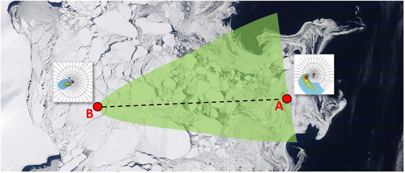
Figure 1 Wave propagation in the marginal ice zone. Background photo is a MODIS Terra image from April 23, 2022 (source: https://worldview.earthdata.nasa.gov/), showing a fragment of the MIZ along the eastern coast of Greenland. The cartoon in the foreground illustrates transformation of the wave energy spectra (insets) along a line AB oriented along the mean wave direction. In a ‘standard’ way, the apparent attenuation between A and B is computed from Equation (2), i.e., based on wave energy at A and B only; in reality, the spectrum at B is a net effect of wave energy production, redistribution and dissipation within the green-shaded area.

The above is true, of course, independently of whether sea ice is present at a given location or not. If it is present, however, the situation is particularly challenging as the list of variables that influence wave energy sources and sinks, and thus the dimensionality of a model’s parameter space, is much longer than in open water. It includes ice concentration, thickness and floe size distribution, top and bottom surface roughness, and a set of ice mechanical properties. Moreover, the presence of open-water patches, typical of the MIZ, means that waves propagate through a mosaic of (different types of) ice and water – a complex medium in which the net generation, propagation and dissipation of wave energy is likely different than in each individual component of that mixture alone. This complexity generally tends to be underappreciated by the wave-in-ice modeling community. The rest of this paper discusses challenges that it brings and possible ways out towards more reliable models.

3 Observations and interpretation of wave attenuation in sea ice

Waves in sea ice are measured using several different techniques, including, but not limited to, in situ observations by means of buoys or accelerometers placed on the ice (e.g., Squire and Moore, 1980; Cheng et al., 2017; Voermans et al., 2019; Kohout et al., 2020; Wahlgren et al., 2023), analysis of ship motion (e.g., Collins et al., 2015), remote observations from ships by stereo imaging (e.g., Smith and Thomson, 2019; Alberello et al., 2022) and from aircrafts by laser scanning (Sutherland and Gascard, 2016; Sutherland et al., 2018), satellite-based methods (e.g., Stopa et al., 2018a, b; Horvat et al., 2020; Brouwer et al., 2022; Huang and Li, 2023), or, recently, distributed acoustic sensing of seafloor cables (Smith et al., 2023). Taken together, the result of this observational effort is a large, very valuable body of data encompassing thousands of measured wave energy spectra. However, as will be argued below, several factors limit the usefulness of large parts of that data for formulating models of wave evolution in sea ice, independently of whether these models are data-based or physics-based. The associated problems can be broadly divided into two groups, the first one related to the determination of wave energy changes with distance, and the second – to the attribution of those changes to particular combinations of ice properties and forcing acting on it.

Many of the problems from the first group are related to the limited number of locations at which observations are made. Even extensive field campaigns (e.g., Cheng et al., 2017) are limited to a few data points. SAR- and other satellite-based studies rely on very-high resolution imagery, which typically has small spatial extent, so that often only a single energy spectrum per image can be derived (as, e.g., in Stopa et al., 2018b, who compared a single spectrum per satellite image with a corresponding open-ocean spectrum from a numerical wave model). As a result, analyses based on that data reduce to comparisons of spectra from two data points (notably, even if more than two buoys are used, they are often analyzed on a pairwise basis, as in, e.g., Cheng et al., 2017; Kohout et al., 2020; Montiel et al., 2022). If we denote those two locations by A and B, then the so-called apparent attenuation coefficient α_a is computed as (e.g., Stopa et al., 2018b; Kohout et al., 2020; Alberello et al., 2022; Montiel et al., 2022):

$\begin{array}{ll}{\alpha }_a=-\frac{\text{log }(E_B/E_A)}{d_{AB}},& (2)\end{array}$

where E_A and E_B denote the energy of a given spectral component at A and B, respectively, and d_AB is the distance between A and B (corrected for wave propagation direction). Thus, α_a represents the net change of the energy of that component along the line segment AB. As already discussed, this change depends on the sum of all processes shaping the energy spectra over a large area up-wave from B. Crucially, the assumption underlying Equation (2) is an exponential change of wave energy with distance x:

$\begin{array}{ll}dE/dx=-{\alpha }_{a}E.& (3)\end{array}$

Although many studies claim that observations consistently show exponential wave attenuation in sea ice, the solid observational evidence for Equation (3) is in fact rather limited. Only very few papers actually present least-square fits of Equation (3) to observational data – which, obviously, requires several data points that can be fitted. Even fewer studies consider alternative forms of dE/dx. Good fit with Equation (3) was reported for field data by Squire and Moore (1980) and most, but not all cases in Wadhams et al. (1988). Stopa et al. (2018a) found difficulties in fitting single exponential curves to their SAR-derived wave heights and opted for piecewise fitting instead, with two very different exponential curves close to the ice edge and deeper inside of the MIZ. Strong dependence of attenuation on distance from the ice edge was also found by Hošeková et al. (2020). Recently, Huang and Li (2023) fitted exponential curves to satellite-derived profiles of wave heights (consisting of more than 10 data points), but high scatter in their data makes it difficult to estimate whether other functional forms would provide a better fit. Also, both Stopa et al. (2018a) and Huang and Li (2023) analyzed changes of the total wave energy (i.e., significant wave height), so that nothing can be said about frequency-dependent attenuation based on their data. The evidence for linear attenuation, at least in some cases, was reported by Montiel et al. (2018) and Brouwer et al. (2022). Herman et al. (2019) found non-exponential attenuation in laboratory data. On theoretical grounds, some physical mechanisms of wave attenuation lead to an exponential change of wave energy with distance (e.g., scattering; Montiel et al., 2016), and some do not (e.g., turbulent dissipation in the under-ice boundary layer; Kohout et al., 2011; Herman, 2021). Thus, Equation (3) should not be seen as a universal attenuation model for sea ice, valid in all ice and forcing conditions.

It is often argued that even though individual physical processes affecting wave propagation in sea ice might produce non-exponential, spatially varying attenuation, their net effect over sufficiently large distances can be well approximated with an exponential curve (see, e.g., Shen, 2022). Considering the problems with the apparent attenuation described above, the urgent question is not whether this statement is true or not, but rather – even if it is true – whether such “long-distance attenuation” might be useful for spectral wave modeling. Is it a promising concept that might lead to improved predictive power of models, or to an improved understanding of sea ice and wave physics? It is very unlikely. Attenuation coefficients averaged over long distances, time periods and ice types might provide a stable estimate of an “effective” attenuation in a given area, as showed by Voermans et al. (2022), but it is hard to imagine how such an estimate, based on a single-transect approach and very specific assumptions (unidirectional waves, exponential attenuation, etc.), could be used to construct an input for a spectral wave model, i.e., a map of attenuation coefficients over a large area that must be valid for arbitrary wave directions and propagation paths under time-varying forcing. Such an approach might be useful for computing rough estimates of the MIZ width, or, possibly, for climate modeling, but definitely not at synoptic and similar time scales, when the goal is to reproduce details of a single weather event and to capture changes in attenuation related, e.g., to a sudden ice breakup (Collins et al., 2015; Ardhuin et al., 2020) or temporal variability of wind speed and direction. Rabault et al. (2024) demonstrated recently how sensitive wave evolution in sea ice is to short-term fluctuations of sea ice properties and forcing.

In fact, the usage of apparent attenuation computed over large distances makes the problems from the second group mentioned above even worse. The larger the distance over which the apparent attenuation is computed, the more likely the assumption of homogeneous conditions is violated (the size of the green area in Figure 1 increases), the larger the number of factors that potentially contribute to the net wave evolution, and the more difficult it is to collect relevant data on ice properties, without which the observed net attenuation rates cannot be interpreted in any way useful for formulating ice-related source terms. On top of all that, long-distance attenuation can be measured only when attenuation rates are sufficiently low so that the wave energy at both ends of the analyzed profile is higher than the noise level associated with the measuring technique used. This is particularly problematic for short waves and may lead to various spurious effects in the estimated attenuation rates (e.g., Thomson et al., 2021).

4 Spectral wave modeling in sea ice

If sea ice is present in a given grid cell of a spectral wave model, several terms in the energy balance Equation (1) might change, depending on ice type and properties. On the left-hand side of Equation (1), if the dispersion relation differs from that valid in open water, the group velocity is different and, if ice properties vary in space, c_θ is nonzero leading to refraction. Hence, $D_{\text{ice}}E/Dt$ replaces $DE/Dt$. On the right-hand side of Equation (1), the modifications are twofold. First, the form of all three groups of source terms might be different in ice-covered and ice-free areas. Second, new source terms might be necessary to represent physical processes specific for sea ice, which are absent in open water. We have:

$\begin{array}{ll}\frac{D_{\text{ice}}E}{Dt}=(1-A)(S_{\text{in}}+S_{\text{nl}}+S_{\text{ds}})+A(S_{\text{in},\text{ice}}+S_{\text{nl},\text{ice}}+S_{\text{ds},\text{ice}}+S_{\text{sc},\text{ice}}+S_{\text{dsi},\text{ice}}),& (4)\end{array}$

where A denotes ice concentration, $S_{\text{in},\text{ice}}$, $S_{\text{nl},\text{ice}}$ and $S_{\text{ds},\text{ice}}$ are analogous to $S_{\text{in}}$, $S_{\text{nl}}$ and $S_{\text{ds}}$, i.e., represent wind input, wave–wave interactions and dissipation in ice by processes analogous to those present in open water (e.g., deep-water wave breaking), $S_{\text{sc},\text{ice}}$ denotes a source term representing scattering, and $S_{\text{dsi},\text{ice}}$ is a group of source terms describing all ice-specific dissipation mechanisms (e.g., viscous dissipation, floe breaking, floe collisions, etc.). An assumption behind Equation (4), made in essentially all spectral-modeling studies, is that the net effect of all physical processes modifying the energy spectrum in an area (a model grid cell) covered with a mosaic of ice and water can be computed as a linear combination of contributions from ice and water, disregarding their subgrid-scale spatial pattern. Another assumption is that $S_{\text{in},\text{ice}}$, $S_{\text{nl},\text{ice}}$ and $S_{\text{dsi},\text{ice}}$ are simply scaled versions of $S_{\text{in}}$, $S_{\text{nl}}$ and $S_{\text{ds}}$, respectively, that is:

$\begin{array}{ll}\frac{D_{\text{ice}}E}{Dt}=(1-A+a_{\text{in}}A)S_{\text{in}}+(1-A+a_{\text{nl}}A)S_{\text{nl}}+(1-A+a_{\text{ds}}A)S_{\text{ds}}+A(S_{\text{sc},\text{ice}}+S_{\text{dsi},\text{ice}}),& (5)\end{array}$

where a_in, a_nl and a_ds are constant coefficients. Usually, they are treated in a binary manner, i.e., they are assigned a value of 0 or 1, which amounts to switching the respective processes on or off (e.g., Rogers et al., 2016; Liu et al., 2020). For instance, the default setting in SWAN is $a_{in}=0$ and $a_{ds}=a_{nl}=1$ (SWAN Team, 2022), and in WaveWatchIII $a_{in}=a_{ds}=0$ and $a_{nl}=1$ (WAVEWATCH III Development Group, 2019). Generally, treating a_in, a_nl, a_ds as binary switches reflects our limited understanding of the underlying physics. Recently, acknowledging the fact that the wind input over ice is likely reduced compared to that over open water, but not zero (see, e.g., Rogers et al., 2016), Cooper et al. (2022) arbitrarily set a_in = 0.5 and showed that locally generated waves have a considerable impact on wave evolution in the MIZ. Based on theoretical arguments, Herman and Bradtke (2024) argued for a_in = 0.56, a_nl = a_ds = 1 in fetch-limited, strongly forced waves in coastal polynyas with frazil streaks, and demonstrated that this combination of source terms allows to reproduce observed wave growth patterns there. Importantly, they also showed that, in a general case, a_in is not a constant, but depends on wave frequency and wind speed.

As for the ice-specific source terms, physics-based parameterizations suitable for direct implementation in spectral wave models have been formulated for energy-redistribution by scattering ($S_{\text{sc},\text{ice}}$; Meylan and Bennetts, 2018), with some serious limitations as discussed in (Montiel et al., 2024); for turbulent, floe-size dependent dissipation in the under-ice boundary layer (Herman, 2021); and for flexural and viscoelastic damping (see Shen, 2022, and references therein). In most applications, however, the net $S_{\text{dsi},\text{ice}}$ is parameterized as a simple power series $S_{sc,\text{ice}}=c_g{\alpha }_{\text{ice}}E$ with ${\alpha }_{\text{ice}}={\sum }_n{\alpha }_n{f}^n$ and one or more coefficients α_n different from zero (α_n are either constant or dependent on ice thickness, see, e.g., Rogers et al., 2018a, Rogers et al., 2018b, for an overview). The values of n predicted by theoretical models of individual physical processes generally tend to be much higher than observed ones, which usually lie in the range 2<n<4 (Meylan et al., 2018).

5 A simple numerical experiment

Let us consider a very simple numerical experiment, in which the apparent attenuation coefficients are computed from the results of a few runs of a spectral wave model set up for an idealized, one-dimensional MIZ (Figure 2; details of simulations can be found in the Supplementary Material). The model is run N_r = 6 times with arbitrarily set values a_in = 0.5 (as in Cooper et al., 2022), $a_{\text{nl}}=a_{\text{d}\text{s}}=1$ and ${\alpha }_{\text{ice}}\sim f^5$, for very weak, moderate and strong wind forcing. For each one of the N_r resulting wave energy profiles $E(x_1,f)$, a series of α_a values is computed from Equation (2), for varying d_AB. As can be seen (color points in Figure 2), in spite of the very small number of cases tested, a remarkably broad cloud of α_a values is obtained, depending on input energy spectra, wind speed and, crucially, “measurement” locations. Without doubt, N_r is too small for any statistical analysis, and the results are sensitive to the particular model settings used. Nevertheless, this simple example provides very instructive insights. First, at all frequencies ${\alpha }_a<{\alpha }_{\text{ice}}$, and the differences tend to increase with increasing d_AB: the further points A and B are from each other, the poorer approximation of α_ice is obtained from α_a. Thus, the upper envelope of α_a values seems to provide a better estimate of α_ice than the mean. When the mean α_a over all observations is used, the resulting slope of the ${\overline{\alpha }}_a(f)$ curve is much lower than α_ice (3.2 versus 5.0 in our example). α_a is close to α_ice only for swell waves with very narrow directional and frequency spreading, and at small distances. Notably, as each of the S_in, S_nl and S_ds terms has its own spectral characteristics, different frequency bands have different sensitivity to the “action” of these terms, which in turn influences differences between α_ice and α_a.

Figure 2

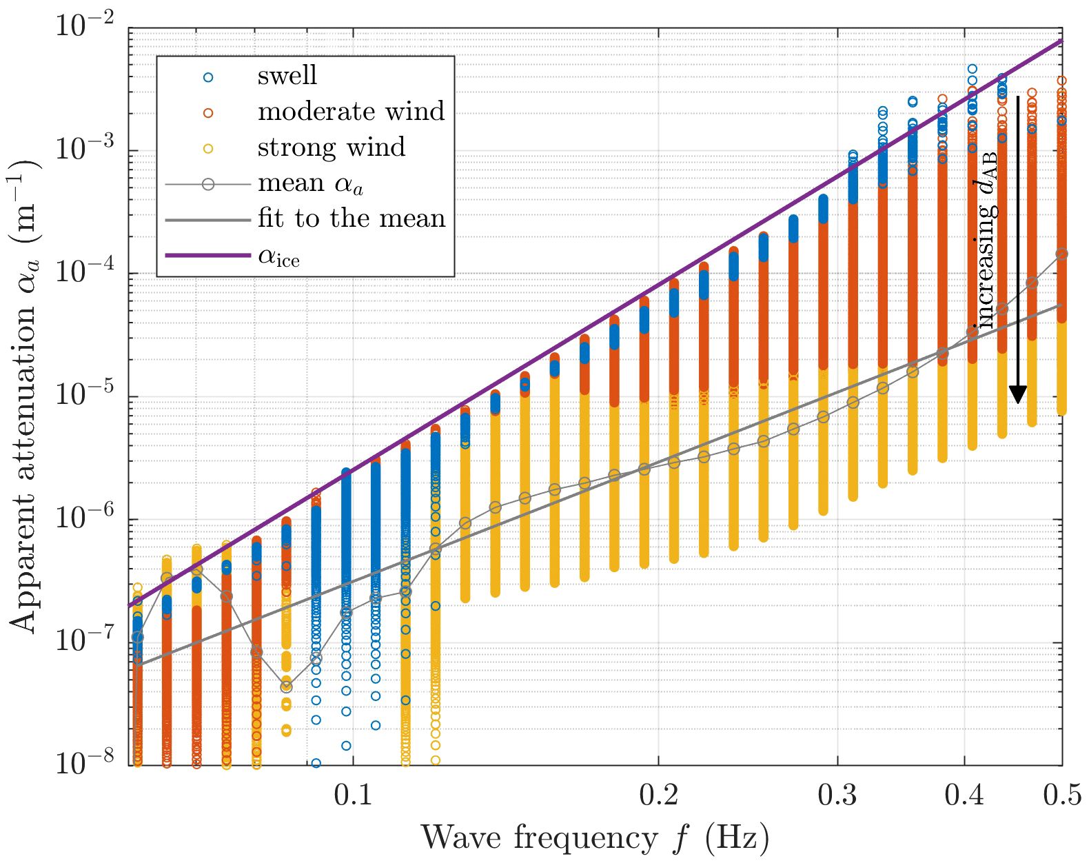
Figure 2 Apparent attenuation “observed” in the results of a simple, one-dimensional spectral wave model run with a constant ice concentration and wind speed, as described in the Supplementary Information. There are seven model runs grouped into three wind speed classes. Color circles represent α_a computed as in Equation (2), between point A at the model boundary and point B located at distance d_AB between 500 m and 500 km from A. The mean ${\overline{\alpha }}_a(f)$ is shown with gray circles, and the gray line is a least-square fit to ${\overline{\alpha }}_a(f)$; it has a slope 3.2. The thick violet line shows ${\alpha }_{ice}(f)$ used in the S_ice term in the model. Note that the clouds of points of different colors overlap.

Considering the complexity present in this highly idealized case, it is easy to imagine how difficult is an inverse task of finding α_ice based on measured spectra from just two points (e.g., Rogers et al., 2016), with incomplete data on ice properties, and the unknown form of S_ice, a_in, a_nl, a_ds and possibly several other terms on the right-hand-side of Equation (5).

6 Discussion: towards more versatile wave models for ice-covered seas

Remarkably, many of the problems described so far have been identified already in 1980s (e.g., Wadhams et al., 1988). The fact that after more than three decades of research we are still far from solving them suggests that a change of perspective might be necessary, because our efforts so far – in spite of many successes – have led to only limited improvements in the performance of spectral models in sea ice. Undoubtedly, one of the most important factors limiting the progress is the lack or incompleteness of information on ice properties accompanying wave measurements. In many cases, ice concentration is the only known variable, possibly combined with some estimates of ice type and thickness. Thus, laboratory-and model-supported estimates of the relevant model parameters seem particularly valuable (e.g., Cheng et al., 2018; Herman et al., 2019, and many others), as are insights from coupled wave–ice models (e.g., Boutin et al., 2018; Roach et al., 2019, 2020). Obviously, however, the models are only as good as the parameterizations used in them.

Based on our wave-in-ice modeling experience so far, it seems reasonable to formulate the following guidelines for further research:

● There are no reasons to assume that just one physical mechanism of wave energy attenuation in ice dominates over others. The often repeated question “scattering or dissipation?” is misleading. Although our understanding of processes accompanying wave evolution in sea ice is far from complete, we do have enough evidence to acknowledge that both scattering and several different dissipative processes lead to wave energy attenuation in sea ice, in proportions that depend on ice and forcing conditions, i.e., vary in space and time. Moreover, energy input and wave–wave interactions do play a role as well, especially when ice concentration A<1 (see Herman and Bradtke, 2024, for an example of a net wave growth in ice). Thus, it is generally more appropriate to speak of wave evolution rather than wave attenuation in sea ice.

● Accordingly, calibrating models representing a single physical process to observations should be avoided, especially if it requires setting unrealistic values to physically meaningful coefficients (ice bottom roughness, shear modulus, etc.). Many researchers, including the author of this paper, have done that in spite of being fully aware of the flaws of this approach (e.g., Cheng et al., 2017; Herman, 2021). Instead, we should try to constrain values of coefficients based on dedicated, theory-supported laboratory and field observations, and thus estimate the relative contribution of a given process to the total observed energy dissipation under a given combination of conditions. The works by Boutin et al. (2018); Voermans et al. (2019), or Smith and Thomson (2020) are very good examples of this approach.

● Theoretical models describing physical mechanisms of wave energy dissipation in sea ice are often judged by the value of the power n (in the relationship ${\alpha }_{\text{ice}}\sim f^n$) they predict, and $n\gg 4$ is considered an argument against a given physical process as a candidate to explain the observed attenuation (Meylan et al., 2018). Vice versa, models predicting 2<n<4 are regarded as promising. However, this reasoning disregards, first, the difference between the apparent attenuation α_a and the ice-related attenuation α_ice, which might have different frequency dependence (recall the numerical experiment above), and second, the fact that the physical process described by a given model might account for just a small fraction of the total observed attenuation. Thus, at least some models with relatively high n might be much better than their value of n suggests.

● Depending on the relative contributions of all source terms on the right-hand side of Equation (5), the shape of the resulting attenuation curves might be different. In situations when linear processes (e.g. scattering) dominate, exponential attenuation can be expected, but there is no reason why this shape should be universal. It is quite remarkable how strong the wave-in-ice community’s attachment towards exponential attenuation is. The treatment of turbulent dissipation under the ice is a very good example. Turbulence is an inherently nonlinear process. Nevertheless, in their seminal paper Liu and Mollo-Christensen (1988) attempted to account for it by simply replacing the molecular viscosity of water with a constant eddy viscosity, disregarding the dependence of the latter on flow conditions, that is, in this case, on wave amplitude. Kohout et al. (2011) showed that nonlinear ice–water drag leads to non-exponential attenuation, but decided to approximate the resulting wave profiles with exponential curves. Later, Stopa et al. (2016) and Boutin et al. (2018) used a nonlinear model, with an attenuation coefficient dependent on wave energy through its dependence on the amplitude of wave orbital velocity, but failed to recognize that nonlinearity in the analysis and interpretation of their results. Crucially, as noted earlier, spectral models do not rely on any assumptions about the form of the “long distance” attenuation, and any functional form of the ice-related source terms, including their linear or nonlinear dependence on wave energy, can be handled without problems.

● More attention should be directed towards wave generation and wave–wave interactions in (partial) ice cover. Only very few studies concentrate on the theory of wave growth (Zhao and Zhang, 2020) and nonlinear energy transfer (Polnikov and Lavrenov, 2007; Pierce et al., 2024) in sea ice, in spite of clear evidence that these processes are important, especially under high-wind conditions (Li et al., 2015; Cooper et al., 2022; Herman and Bradtke, 2024).

● The difference between α_a and α_ice must be taken into account by calibration of spectral wave models to observational data. The task is to find the functional form and values of parameters not only of the $S_{\text{dsi},\text{i}}$ term, but all terms on the right-hand side of Equation (5). The fact that so far this is done for just a small subset of parameters, with others arbitrarily kept constant, explains the very large scatter of fitted α_ice values in model calibration studies (e.g., Rogers et al., 2016). The high number of dimensions of the parameter space is the major challenge that cannot be avoided, independently of whether physics-based or data-based (Rogers et al., 2021; Yu et al., 2022) models are used.

The last point on the list brings us back to the issue of observational data necessary to face the challenges. The experience so far shows, not surprisingly, that even in simple laboratory settings many different combinations of adjustable coefficients can reproduce observations if those are limited to profiles of wave amplitude (Herman et al., 2019). Thus, observations of apparent attenuation are useful for model validation, whereas model development seems feasible only with dedicated measurements of possibly large number of variables collected under relatively straightforward conditions and informed by theory.

Data availability statement

The original contributions presented in the study are included in the article/Supplementary Material. Further inquiries can be directed to the corresponding author.

Author contributions

AH: Conceptualization, Funding acquisition, Project administration, Visualization, Writing – original draft, Writing – review & editing.

Funding

The author(s) declare financial support was received for the research, authorship, and/or publication of this article. This work has been financed by Polish National Science Centre project no. 2022/47/B/ST10/01129 (“Sea ice, waves and turbulence – from laboratory scale to improved large-scale modeling”).

Acknowledgments

We acknowledge the use of imagery from the NASA Worldview application (https://worldview.earthdata.nasa.gov), part of the NASA Earth Observing System Data and Information System (EOSDIS).

Conflict of interest

The author declares that the research was conducted in the absence of any commercial or financial relationships that could be construed as a potential conflict of interest.

Publisher’s note

All claims expressed in this article are solely those of the authors and do not necessarily represent those of their affiliated organizations, or those of the publisher, the editors and the reviewers. Any product that may be evaluated in this article, or claim that may be made by its manufacturer, is not guaranteed or endorsed by the publisher.

Supplementary material

The Supplementary Material for this article can be found online at: https://www.frontiersin.org/articles/10.3389/fmars.2024.1413116/full#supplementary-material

References

Alberello A., Bennetts L., Onorato M., Vichi M., MacHutchon K., Eayrs C., et al. (2022). Three-dimensional imaging of waves and floes in the marginal ice zone during a cyclone. Nat. Commun. 13, 4590. doi: 10.1038/s41467-022-32036-2

PubMed Abstract | CrossRef Full Text | Google Scholar

Ardhuin F., Otero M., Merrifield S., Grouazel A., Terrill E. (2020). Ice breakup controls dissipation of wind waves across Southern Ocean sea ice. Geophys. Res. Lett. 47, e2020GL087699. doi: 10.1029/2020GL087699

CrossRef Full Text | Google Scholar

Boutin G., Ardhuin F., Dumont D., Sévigny C., Girard-Ardhuin F., Accensi M. (2018). Floe size effect on wave–ice interactions: possible effects, implementation in wave model, and evaluation. J. Geophys. Res. 123, 13622. doi: 10.1029/2017JC013622

CrossRef Full Text | Google Scholar

Boutin G., Lique C., Ardhuin F., Rousset C., Talandier C., Accensi M., et al. (2020). Towards a coupled model to investigate wave–sea ice interactions in the Arctic marginal ice zone. Cryosphere 14, 709–735. doi: 10.5194/tc-14-709-2020

CrossRef Full Text | Google Scholar

Brouwer J., Fraser A., Murphy D., Wongpan P., Alberello A., Kohout A., et al. (2022). Altimetric observation of wave attenuation through the Antarctic marginal ice zone using ICESat-2. Cryosphere 16, 2325–2353. doi: 10.5194/tc-16-2325-2022

CrossRef Full Text | Google Scholar

Cavaleri L., Abdalla S., Benetazzo A., Bertotti L., Bidlot J.-R., Breivik Ø., et al. (2018). Wave modelling in coastal and inner seas. Prog. Oceanogr. 167, 164–233. doi: 10.1016/j.pocean.2018.03.010

CrossRef Full Text | Google Scholar

Cheng S., Rogers W., Thomson J., Smith M., Doble M., Wadhams P., et al. (2017). Calibrating a viscoelastic sea ice model for wave propagation in the Arctic fall marginal ice zone. J. Geophys. Res. 122, 8740–8793. doi: 10.1002/2017JC013275

CrossRef Full Text | Google Scholar

Cheng S., Tsarau A., Evers K.-U., Shen H. (2018). Floe size effect on gravity wave propagation through ice covers. J. Geophys. Res. 124, 320–334. doi: 10.1029/2018JC014094

CrossRef Full Text | Google Scholar

Collins C., Rogers W., Marchenko A., Babanin A. (2015). In situ measurements of an energetic wave event in the Arctic marginal ice zone. Geophys. Res. Lett. 42, 1863–1870. doi: 10.1002/2015GL063063

CrossRef Full Text | Google Scholar

Cooper V., Roach L., Thomson J., Brenner S., Smith M., Meylan M., et al. (2022). Wind waves in sea ice of the western Arctic and a global coupled wave–ice model. Phil. Trans. R. Soc A 380, 20210258. doi: 10.1098/rsta.2021.0258

CrossRef Full Text | Google Scholar

Dumont D. (2022). Marginal ice zone dynamics: history, definitions and research perspectives. Phil. Trans. R. Soc A 380, 20210253. doi: 10.1098/rsta.2021.0253

CrossRef Full Text | Google Scholar

Herman A. (2021). Spectral wave energy dissipation due to under-ice turbulence. J. Phys. Oceanogr. 51, 1177–1186. doi: 10.1175/JPO-D-20-0171.1

CrossRef Full Text | Google Scholar

Herman A., Bradtke K. (2024). Fetch-limited, strongly forced wind waves in waters with frazil and grease ice – spectral modelling and satellite observations in an Antarctic coastal polynya. J. Geophys. Res. 129, e2023JC020452. doi: 10.1029/2023JC020452

CrossRef Full Text | Google Scholar

Herman A., Cheng S., Shen H. (2019). Wave energy attenuation in fields of colliding ice floes. Part 2: A laboratory case study. Cryosphere 13, 2901–2914. doi: 10.5194/tc-13-2901-2019

CrossRef Full Text | Google Scholar

Holthuijsen L. (2007). Waves in oceanic and coastal waters (Cambridge, UK: Cambridge Univ. Press), 387 pp.

Google Scholar

Horvat C. (2022). Floes, the marginal ice zone and coupled wave–sea-ice feedbacks. Phil. Trans. R. Soc A 380, 20210252. doi: 10.1098/rsta.2021.0252

CrossRef Full Text | Google Scholar

Horvat C., Blanchard-Wrigglesworth E., Petty A. (2020). Observing waves in sea ice with ICESat-2. Geophys. Res. Lett. 47, e2020GL087629. doi: 10.1029/2020GL087629

CrossRef Full Text | Google Scholar

Hošeková L., Malila M., Rogers W., Roach L., Eidam E., Rainville L., et al. (2020). Attenuation of ocean surface waves in pancake and frazil sea ice along the coast of the Chukchi Sea. J. Geophys. Res. 125, e2020JC016746. doi: 10.1029/2020JC016746

CrossRef Full Text | Google Scholar

Huang B., Li X.-M. (2023). Wave attenuation by sea ice in the Arctic marginal ice zone observed by spaceborne SAR. Geophys. Res. Lett. 50, e2023GL105059. doi: 10.1029/2023GL105059

CrossRef Full Text | Google Scholar

Kohout A., Meylan M., Plew D. (2011). Wave attenuation in a marginal ice zone due to the bottom roughness of ice floes. Ann. Glaciol. 52, 118–122. doi: 10.3189/172756411795931525

CrossRef Full Text | Google Scholar

Kohout A., Smith M., Roach L., Williams G., Montiel F., Williams M. (2020). Observations of exponential wave attenuation in Antarctic sea ice during the PIPERS campaign. Ann. Glaciol. 61, 196–209. doi: 10.1017/aog.2020.36

CrossRef Full Text | Google Scholar

Li J., Kohout A., Shen H. (2015). Comparison of wave propagation through ice covers in calm and storm conditions. Geophys. Res. Lett. 42, 5935–5941. doi: 10.1002/2015GL064715

CrossRef Full Text | Google Scholar

Liu A., Mollo-Christensen E. (1988). Wave propagation in a solid ice pack. J. Phys. Oceanogr. 18, 1702–1712. doi: 10.1175/1520-0485(1988)018<1702:WPIASI>2.0.CO;2

CrossRef Full Text | Google Scholar

Liu Q., Rogers W., Babanin A., Li J., Guan C. (2020). Spectral modeling of ice-induced wave decay. J. Phys. Oceanogr. 50, 1583–1604. doi: 10.1175/JPO-D-19-0187.1

CrossRef Full Text | Google Scholar

Meylan M., Bennetts L. (2018). Three-dimensional time-domain scattering of waves in the marginal ice zone. Phil. Trans. R. Soc A 376, 20170334. doi: 10.1098/rsta.2017.0334

CrossRef Full Text | Google Scholar

Meylan M., Bennetts L., Mosig J., Rogers W., Doble M., Peter M. (2018). Dispersion relations, power laws, and energy loss for waves in the marginal ice zone. J. Geophys. Res. 123, 3322–3335. doi: 10.1002/2018JC013776

CrossRef Full Text | Google Scholar

Montiel F., Kohout A., Roach L. (2022). Physical drivers of ocean wave attenuation in the marginal ice zone. J. Phys. Oceanogr. 52, 889–906. doi: 10.1175/JPO-D-21-0240.1

CrossRef Full Text | Google Scholar

Montiel F., Meylan M., Hawkins S. (2024). Scattering kernel of an array of floating ice floes: application to water wave transport in the marginal ice zone. Proc. R. Soc A 480, 20230633. doi: 10.1098/rspa.2023.0633

CrossRef Full Text | Google Scholar

Montiel F., Squire V., Bennetts L. (2016). Attenuation and directional spreading of ocean wave spectra in the marginal ice zone. J. Fluid Mech. 790, 492–522. doi: 10.1017/jfm.2016.21

CrossRef Full Text | Google Scholar

Montiel F., Squire V., Doble M., Thomson J., Wadhams P. (2018). Attenuation and directional spreading of ocean waves during a storm event in the autumn Beaufort Sea marginal ice zone. J. Geophys. Res. 123, 5912–5932. doi: 10.1029/2018JC013763

CrossRef Full Text | Google Scholar

Pierce M., Liu Y., Yue D. (2024). Sum-frequency triad interations among surface waves propagating through an ice sheet. J. Fluid Mech. 980, A45. doi: 10.1017/jfm.2024.44

CrossRef Full Text | Google Scholar

Polnikov V., Lavrenov I. (2007). Calculation of the nonlinear energy transfer through the wave spectrum at the sea surface covered with broken ice. Oceanology 47, 334–343. doi: 10.1134/S0001437007030058

CrossRef Full Text | Google Scholar

Rabault J., Halsne T., Carrasco A., Korosov A., Voermans J., Bohlinger P., et al. (2024). In-situ observations of strong waves in ice amplitude modulation with a 12-hour period: a likely signature of complex physics governing waves in ice attenuation? arXiv. doi: 10.48550/arXiv.2401.07619

CrossRef Full Text | Google Scholar

Roach L., Bitz C., Horvat C., Dean S. (2019). Advances in modeling interactions between sea ice and ocean surface waves. J. Adv. Mod. Earth Syst. 11, 4167–4181. doi: 10.1029/2019MS001836

CrossRef Full Text | Google Scholar

Rogers W., Meylan M., Kohout A. (2018a). Frequency distribution of dissipation of energy of ocean waves by sea ice using data from Wave Array 3 of the ONR “Sea State” field experiment (USA: Naval Research Laboratory), 32 pp. Tech. Rep. NRL/MR/7322–18-9801.

Google Scholar

Rogers W., Meylan M., Kohout A. (2021). Estimates of spectral wave attenuation in Antarctic sea ice, using model/data inversion. Cold Regions Sci. Tech. 182, 103198. doi: 10.1016/j.coldregions.2020.103198

CrossRef Full Text | Google Scholar

Rogers W., Posey P., Li L., Allard R. (2018b). Forecasting and hindcasting waves in and near the marginal ice zone: wave modeling and the ONR “Sea State” field experiment (USA: Naval Research Laboratory), 183 pp. Tech. Rep. NRL/MR/7320–18-9786.

Google Scholar

Rogers W., Thomson J., Shen H., Doble M., Wadhams P., Cheng S. (2016). Dissipation of wind waves by pancake and frazil ice in the autumn Beaufort Sea. J. Geophys. Res. 121, 7991–8007. doi: 10.1002/2016JC012251

CrossRef Full Text | Google Scholar

Shen H. (2022). Wave-in-ice: theoretical bases and field observations. Phil. Trans. R. Soc A 380, 20210254. doi: 10.1098/rsta.2021.0254

CrossRef Full Text | Google Scholar

Smith M., Thomson J. (2019). Ocean surface turbulence in newly formed marginal ice zones. J. Geophys. Res. 124, 1382–1398. doi: 10.1029/2018JC014405

CrossRef Full Text | Google Scholar

Smith M., Thomson J. (2020). Pancake sea ice kinematics and dynamics using shipboard stereo video. Ann. Glaciol. 61, 1–11. doi: 10.1017/aog.2019.35

CrossRef Full Text | Google Scholar

Smith M., Thomson J., Baker M., Abbott R., Davis J. (2023). Observations of ocean surface wave attenuation in sea ice using seafloor cables. Geophys. Res. Lett. 50, e2023GL105243. doi: 10.1029/e2023GL105243

CrossRef Full Text | Google Scholar

Squire V. (2018). A fresh look at how ocean waves and sea ice interact. Phil. Trans. R. Soc A 376, 20170342. doi: 10.1098/rsta.2017.0342

CrossRef Full Text | Google Scholar

Squire V. (2020). Ocean wave interactions with sea ice: A reappraisal. Annu. Rev. Fluid Mech. 52, 37–60. doi: 10.1146/annurev-fluid-010719-060301

CrossRef Full Text | Google Scholar

Squire V., Moore S. (1980). Direct measurement of the attenuation of ocean waves by pack ice. Nature 283, 366–368. doi: 10.1038/283365a0

CrossRef Full Text | Google Scholar

Stopa J., Ardhuin F., Girard-Ardhuin F. (2016). Wave climate in the Arctic 1992–2014: seasonality and trends. Cryosphere 10, 1605–1629. doi: 10.5194/tc-10-1605-2016

CrossRef Full Text | Google Scholar

Stopa J., Ardhuin F., Thomson J., Smith M., Kohout A., Doble M., et al. (2018a). Wave attenuation through an Arctic marginal ice zone on 12 October 2015. 1. Measurement of wave spectra and ice features from Sentinel 1A. J. Geophys. Res. 123. doi: 10.1029/2018JC013791

CrossRef Full Text | Google Scholar

Stopa J., Sutherland P., Ardhuin F. (2018b). Strong and highly variable push of ocean waves on Southern Ocean sea ice. Proc. Nat. Acad. Sci. 115, 5861–5865. doi: 10.1073/pnas.1802011115

CrossRef Full Text | Google Scholar

Sutherland P., Brozena J., Rogers W., Doble M., Wadhams P. (2018). Airborne remote sensing of wave propagation in the marginal ice zone. J. Geophys. Res. 123, 4132–4152. doi: 10.1029/2018JC013785

CrossRef Full Text | Google Scholar

Sutherland P., Gascard J.-C. (2016). Airborne remote sensing of ocean wave directional wavenumber spectra in the marginal ice zone. Geophys. Res. Lett. 43, 5151–5159. doi: 10.1002/2016GL067713

CrossRef Full Text | Google Scholar

SWAN Team (2022). SWAN Cycle III, version 41.45, Scientific and Technical Documentation (Delft, Netherlands: Delft University of Technology, Faculty of Civil Engineering and Geosciences).

Google Scholar

Thomson J. (2022). Wave propagation in the marginal ice zone: connections and feedback mechanisms within the air–ice–ocean system. Phil. Trans. R. Soc A 380, 20210251. doi: 10.1098/rsta.2021.0251

CrossRef Full Text | Google Scholar

Thomson J., Hošeková L., Meylan M., Kohout A., Kumar N. (2021). Spurious rollover of wave attenuation rates in sea ice caused by noise in field measurements. J. Geophys. Res. 126, e2020JC016606. doi: 10.1029/2020JC016606

CrossRef Full Text | Google Scholar

Voermans J., Babanin A., Thomson J., Smith M., Shen H. (2019). Wave attenuation by sea ice turbulence. Geophys. Res. Lett. 46, 6796–6803. doi: 10.1029/2019GL082945

CrossRef Full Text | Google Scholar

Voermans J., Xu X., Babanin A. (2022). Validity of the wave stationarity assumption on estimates of wave attenuation in sea ice: toward a method for wave–ice attenuation observations at global scales. J. Glaciol. 69, 803–810. doi: 10.1017/jog.2022.99

CrossRef Full Text | Google Scholar

Wadhams P., Squire V., Goodman D., Cowan A., Moore S. (1988). The attenuation rates of ocean waves in the marginal ice zone. J. Geophys. Res. 93, 6799–6818. doi: 10.1029/JC093iC06p06799

CrossRef Full Text | Google Scholar

Wahlgren S., Thomson J., Biddle L., Swart S. (2023). Direct observations of wave–sea ice interactions in the Antarctic marginal ice zone. J. Geophys. Res. 128, e2023JC019948. doi: 10.1029/2023JC019948

CrossRef Full Text | Google Scholar

WAVEWATCH III Development Group (2019). User Manual and System Documentation of WAVEWATCH III, version 6.07 (College Park, MD, USA: NOAA/NWS/NCEP/MMAB), 466 pp.

Google Scholar

Yu J., Rogers W., Wang D. (2022). A new method for parameterization of wave dissipation by sea ice. Cold Regions Sci. Tech. 199, 103582. doi: 10.1016/j.coldregions.2022.103582

CrossRef Full Text | Google Scholar

Zhao X., Zhang C. (2020). A theoretical model of wind-wave growth over an ice-covered sea. Boundary Layer Meteorol. 178, 1–19. doi: 10.1007/s10546-020-00552-7

CrossRef Full Text | Google Scholar