Machine learning-based modeling of chl-a concentration in Northern marine regions using oceanic and atmospheric data

Chl-a concentration is one of the key characteristics of marine areas related to photosynthesis, along with oxygen levels and water salinity. Most studies focus on estimating chl-a concentration in closed water bodies, rivers, and coastal areas of the tropical and temperate Earth belts and are therefore limited to specific regions and also require direct measurements and chemical analysis to obtain precise information about marine environmental conditions. Remote sensing techniques and spatial modeling aim to offer tools for rapid and global analysis of climate and ecological changes. In this study, we aim to develop a machine learning (ML)-based approach to estimate chlorophyll-a concentration when satellite data are unavailable. To provide physical parameters that may influence the predicted variable (chl-a concentration), we combined satellite observations from MODIS with geophysical Weather Research & Forecasting (WRF) and Nucleus for European Modelling of the Ocean (NEMO) models. Classical ML and deep learning (DL) algorithms were compared and analyzed for their ability to extract key biogeochemical patterns in the Barents Sea. The proposed approach allows us to forecast chl-a concentration for the next 8 days based on spatial features and measurements from preceding days. The best R² metric achieved was 0.578 using a LightGBM algorithm, confirming the applicability of the developed solution to map the northern marine region even in cases where MODIS observations are unavailable for the preceding period due to insufficient illumination and dense cloud cover.

1 Introduction

Chlorophyll-a (Chl-a) in water is a systemic climate indicator because the pigment is directly related to the functioning of photosynthetic organisms, reflecting the level of photosynthetic activity and the potential of water areas to sequester greenhouse gases from the atmosphere. At the same time, the growth and development of chlorophyll-containing organisms in aquatic environments may vary due to changes in the characteristics of aquatic areas and changes in climatic conditions, particularly temperature regime (Dvoretsky et al., 2023; Pereira et al., 2023). There are methods for estimating chlorophyll concentrations in water using drifting buoys and spot measurements (Hill et al., 2022). However, while these methods are effective for point-based studies, they may not be practical for large-scale monitoring over large areas. Satellite remote sensing allows for large-scale assessment of chl-a concentration, providing continuous monitoring of aquatic ecosystem functioning with a focus on the carbon balance of territories.

Traditional approaches to Chl-a prediction have relied on the use of multivariate statistical regression models that relate remotely sensed data to actual Chl-a measurements (Martinez et al., 2020). Usually, these algorithms use reflectances in chlorophyll-a-associated bands of light, derived from low-level satellite products, and classical ML regression algorithms for modeling (Hu et al., 2021). In modern applications, deep learning algorithms have become the preferred modeling method. This includes heuristics, convolution-based approaches (Ye et al., 2021), and time series forecasting methods that have become widely used for different water bodies’ assessment (Rajaee and Boroumand, 2015; Cho and Park, 2019; Shamshirband et al., 2019).

The northern seas, including the Barents Sea, are the subject of intensive oceanographic and ecological research (Alvarez-Fernandez and Riegman, 2014; Alvera-Azcárate et al., 2021). However, the analysis of Chl-a in these regions is limited by the peculiarities of the northern climate. One of the main difficulties in monitoring chl-a concentrations in the northern oceans, as well as other indices derived from optical sensor measurements, is the limited availability of satellite data. In northern latitudes, most of the year is characterized by short days or even total darkness due to the polar night. Even during the months when sunlight is available, its intensity is insufficient to provide adequate illumination underwater due to the low angle of incidence of the rays. In addition, part of the sea surface is covered by ice in winter, which severely limits the availability of data. As ice melting is a long process, even at the end of the polar night, data cannot be obtained from a large area of the sea surface. Moreover, a dense cloud cover is typical for these regions.

The vast majority of works on prediction of chlorophyll concentration using remote sensing in marine waters are currently presented for tropical and temperate Earth belts, where satellite data are well available (Rousseaux and Gregg, 2017; Cen et al., 2022). Because of the above limitations, the analysis and prediction of chlorophyll concentration in the waters of the North Pole are mainly based on in situ measurements (Desmit et al., 2020), which allow studies only for localized regions. Only a small number of works focused on the determination of chlorophyll concentration in the regions of the north and south poles of the Earth on the basis of remote sensing data. For example, Zhang et al. (2023) propose to use space-based lidar measurements as an alternative data source for predicting chl-a concentration in polar regions. Machine learning approaches have been successfully applied and proven effective in related fields such as environmental, agricultural (Van Klompenburg et al., 2020; Guo et al., 2021, 2022, 2023), and forestry (Illarionova et al., 2022) studies.

Simulation-based approaches exist to estimate chl-a concentrations, one of which is the mechanistic site-based emulation of a global ocean biogeochemical model (MEDUSA) (Hemmings et al., 2015) that can be coupled to the Nucleus for European Modelling of the Ocean (NEMO) (Madec et al., 2017) state-of-the-art ocean model. This method uses statistical and functional relationships with NEMO outputs to estimate the chl-a concentration at the ocean surface. The approach integrates 1-D simulators and statistical uncertainty quantification to predict surface chlorophyll levels based on model parameters. This increases the efficiency of comprehensive parametric analyses, thereby improving the accuracy and reliability of global ocean biogeochemical models such as NEMO. While this approach is expected to yield more accurate predictions compared to the machine learning method, it is also characterized by increased computational complexity and higher time requirements.

To address the existing limitations, this paper proposes a method for predicting 8-day averaged chl-a concentrations in marine areas based on ocean and atmospheric weather data. As a reference data, we use chlorophyll-a measurements derived from the Moderate Resolution Imaging Spectroradiometer (MODIS). We combine Weather Research & Forecasting (WRF), NEMO, and MODIS data to create a new set of features for developing machine learning algorithms further. These data sources are preferred because they provide clues for further predictions, even in the absence of information from spectral satellite observations. The experiments involve two approaches focusing on pixel-based and patch-based forecasting. Machine learning methods based on gradient boosting and deep learning algorithms are considered. The research is carried out for the waters of the Barents Sea.

2 Materials and methods

2.1 Study area

The region of interest covers the Barents Sea and Kara Sea. This area is characterized by distinctive patterns in the dynamics of atmospheric and oceanic processes, which are determined by the geographical location and special properties of the region (Smedsrud et al., 2013). The average depth of the Barents Sea is twice that of the Kara Sea, and the average depth of the Kara Sea is approximately 110 m. The Barents Sea is usually warm and saline enough (due to the circulation of Atlantic currents) to never freeze in winter. On the other hand, the Kara Sea is frozen in winter and covered by thick ice (sometimes reaching 5 m deep). Close to land, there is a strong freshwater outflow and possible biogens that could affect microbial growth. The Novaya Zemlya archipelago influences atmospheric dynamics and produces gusts of cold wind directed towards the continent. During the months of October to February, there is a polar night and the flux of solar radiation is almost zero.

Chl-a concentration values were extracted for the period from 1 January 2019 to 31 December 2022 for an area between the values 23.0° to 71.0° East and 63.0° to 78.0° North. The spatial areas containing the coordinates of the points for which variable values are available from the atmospheric numerical simulation model (WRF) and the ocean numerical simulation model (NEMO) are shown in Figure 1. The intersection of these areas represents the region of interest.

Figure 1

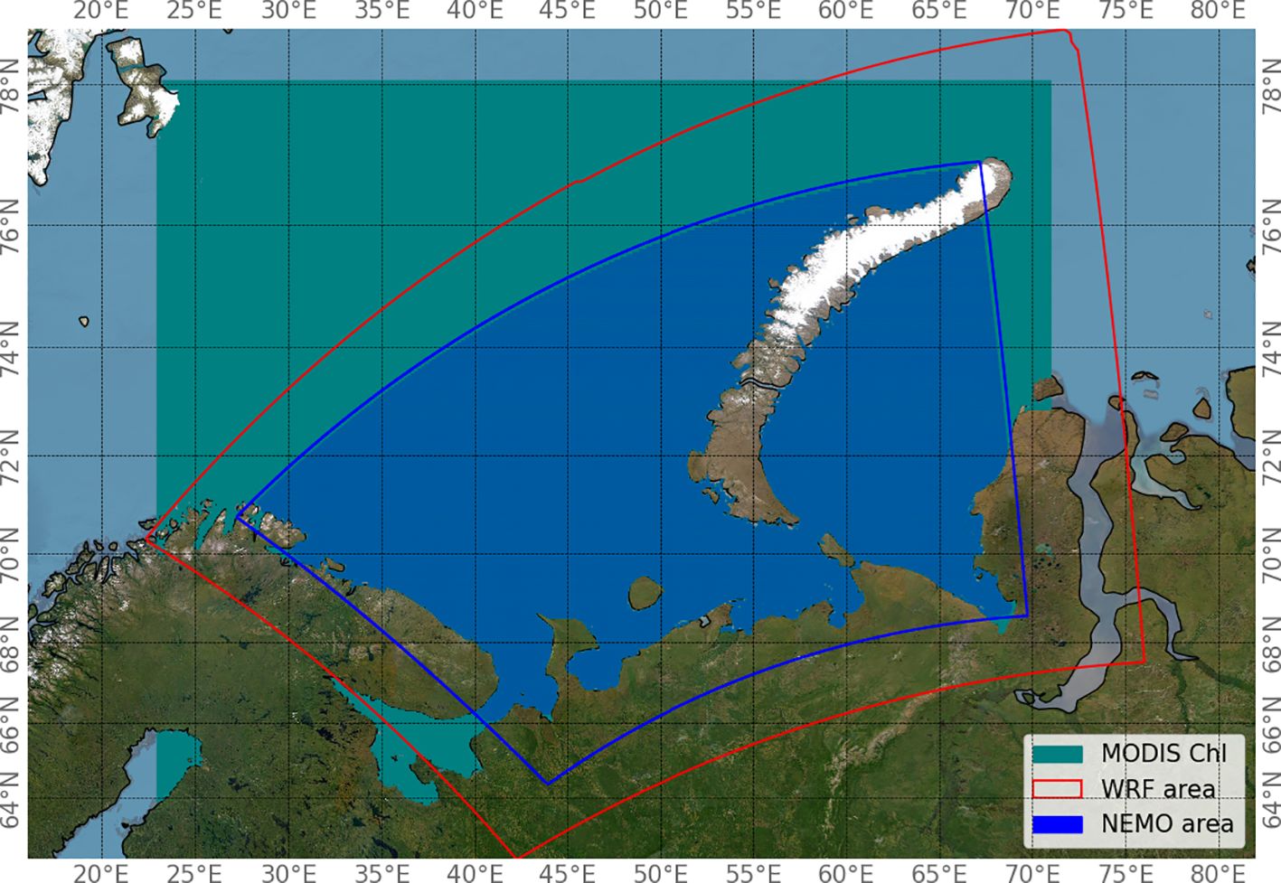
Figure 1 Study area, MODIS spatial data loading domains, and WRF and NEMO simulation domains.

2.2 Data collection

We created a dataset from the outputs of numerical models that we had previously computed—atmospheric numerical simulation based on the WRF (Skamarock et al., 2019) model and ocean numerical simulation based on the NEMO (Madec et al., 2017) model—in order to train the machine learning model to forecast chl-a concentration. Coordinated modeling of ocean and atmosphere can provide coordinated dataset with less mutual numerical instabilities. Furthermore, the data provided by the numerical models are of relatively high spatial resolution compared to the Global Forecast System (GFS) National Centers for Environmental Prediction, National Weather Service, NOAA, U.S. Department of Commerce (2015) and Glorys–Mercator’s ocean data analysis and forecast European Union-Copernicus Marine Service (2016), which are used as initial and boundary conditions for the numerical simulations. Moreover, there is a successful example (Verezemskaya et al., 2021) of configuration of these two particular models in the northern latitudes done in relatively high resolution 1/12° based on the NEMO ORCA12 grid (Barnier et al., 2015). This modeling makes it possible to take into account the influence of additional data, such as the characteristics of atmospheric and ocean dynamic processes on forecasting the concentration of chlorophyll-a.

Chl-a concentration values are derived from the free database of Ocean Biology Distributed Active Archive Center (OB.DAAC) NASA’s Ocean Biology Processing Group (2024), which is based on observations from MODIS. It comprises aggregated satellite Chl-a values in mg/m³, calculated using a combination of color index (CI) (Hu et al., 2019) and ocean color (OC) (O’Reilly and Werdell, 2019) algorithms from an empirical relationship derived from measurements of Chl-a and the blue to green reflectance ratio (R_rs). Geospatial data are available with a pixel size of 4,638 m. In this paper, we get 8-day daily averages of Chl-a from OB.DAAC. The data are presented as two-dimensional arrays of values recorded in netCDF (.nc) format.

A numerical modeling dataset for the atmosphere was obtained using WRF version 4.4.2. WRF is a state-of-the-art atmosphere model designed for both research and numerical weather prediction that allows extensive configuration (Skamarock et al., 2019). As the initial and boundary conditions, the model uses the open source GFS product in the 1/4° resolution. Outputs were calculated in the region of interest from the early 2019 through the end of 2022. We created a local domain configuration and computed the output of the WRF model for the period of interest. The computations took approximately 2 weeks on 360 cores. Outputs contain arrays of 2D and 3D variables with hourly resolution data packed into netCDF files. Every WRF file before preprocessing contains 96 timesteps—24 for the ocean model forcing of the previous day and 72-h forecast. For convenience, data were interpolated from the computational grid to the MODIS grid. WRF files contain the following variables:

● SWDNB—shortwave solar radiation flux near surface,

● LWDNB—longwave solar radiation flux near surface,

● T2—temperature of the air at the height of 2 m,

● RAINNC—accumulated total precipitation near surface,

● U10—U component of the wind speed at a height of 10 m,

● V10—V component of the wind speed at a height of 10 m,

● P—atmospheric pressure at a height of 2 m,

● ALBEDO—albedo coefficient of the surface, and

● Q2—specific air humidity at a height of 2 m.

Numerical modeling dataset of the ocean was calculated with the NEMO (Madec et al., 2017) ocean model version 4.0 with the Drakkar configuration that is created as a joint effort between leading European ocean research facilities (Barnier et al., 2015). This configuration is widely used in the ocean modeling community for high-resolution ocean modeling (Rieck et al., 2015; Verezemskaya et al., 2021). The ocean model was additionally tuned for the region of interest. As initial and boundary conditions for the ocean NEMO uses Glorys and as a forcing (atmospheric boundary conditions), it uses previously computed WRF data. The spatial resolution of the domain is approximately 3–4 km 1/12° and outputs are written every hour. Outputs are represented on the computational grid ORCA12 (Barnier et al., 2015). Local domain configuration and interpolated atmosphere forcing WRF were prepared to run the NEMO ocean model. The calculations took approximately 1 week of CPU time on 128 cores. Data were later interpolated to the MODIS grid, same as the atmosphere model for convenience of use. Outputs are netCDF files with 3D variables that were cut to 2D variables (near surface level values). For the dataset, the following variables are used:

● sosstsst—temperature of the sea water near surface,

● sosaline—salinity of the sea water near surface,

● vozocrtx—U component of currents near surface, and

● vomecrty—V component of currents near surface.

Compared to MODIS data, the unique advantage of WRF and NEMO may be in time scale and the spatial continuity. In order to keep data sources related to each other and because of the daily resolution of MODIS Chl-a data, we took 0-, 24-, 48-, and 72-h time steps of our predictions for WRF and 0- and 24-h time steps for NEMO.

In addition, data on sea ice concentration available in the National Snow and Ice Data Center (Fetterer et al., 2017) database were used. Concentration values were used for data analysis.

2.3 Data preprocessing

The WRF and NEMO numerical simulation data were interpolated onto a grid in a geographic coordinate system corresponding to the MODIS Chl-a product coordinate grid. The preprocessed data were combined into a set of netCDF (.nc) files. Each file in the set contains daily mean chlorophyll concentration values over an 8-day period; NEMO model predictions for days 0, 1, 2, and 3; and WRF model predictions for days 0 and 1. The day with index 0 was taken as the day before this 8-day period. Only points within the NEMO simulation area (the region within the blue border in Figure 1) were used for analysis and modeling.

Time-independent spatial attributes were also used: latitude, longitude, and shortest distance to the coastline, which was calculated for each point within the region of interest. The later dataset was packed into daily files with an 8-day step. The total amount of features was 40, among them:

● 18 WRF features (2 values for each of the 9 features: days 0 and 1),

● 16 NEMO features (4 values for each of the 4 features: days 0, 1, 2, and 3),

● lat—latitude,

● lon—longitude,

● water_depth—water depth,

● coast_dist—shortest distance to the coastline,

● doy—day of the year, and

● chlor_a_prev—Chl-a of the preceding days.

A file structure of the resulting dataset is shown in Figure 2 to illustrate the principle of combining NEMO and WRF modeling data with MODIS data. Figure 3 shows the average number of missing Chl-a values for the region of interest as well as the number of points with high ice concentration (greater than 50%). As can be seen from the figure, the data for the region of interest are completely missing for the months from October to February. These months are the period of insufficient illumination for observations in the visible optical range. For this reason, these months are completely absent from the dataset we collected. Ice formation in the study area begins in November and continues until February, and beginning from March, ice melting occurs. It can be observed that for regions with high ice concentration, observations for chlorophyll concentration values are missing. The remaining omissions are due to other reasons, notably cloud cover.

Figure 2

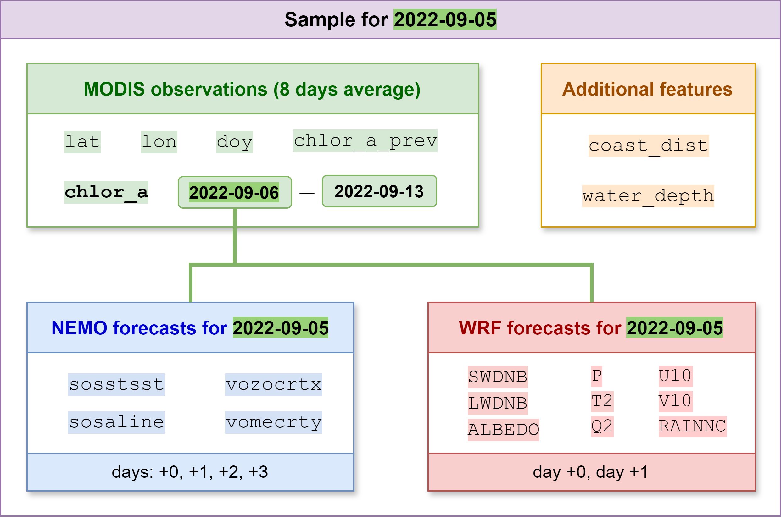
Figure 2 Example of a merged dataset file for a specific observation date.

Figure 3

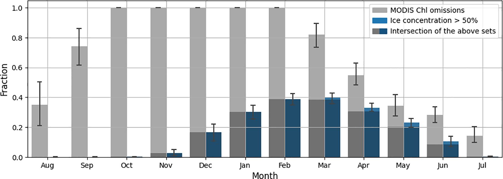
Figure 3 Average proportions of missed MODIS Chl-a values and high ice concentration values in the region of interest by month for the period January 2019 through December 2022.

Figure 4 shows examples of MODIS chlorophyll-a observations extracted for specific dates in 2021 in 32-day increments. By comparing these plots with the distance of the points from the coastline (Figure 5), it is clear that high chlorophyll concentrations are characteristic of coastal areas. It has been long observed in the field that the majority of the world’s most productive marine ecosystems are found within coastal environments and owe their productivity, diversity, and wealth of life to their terrestrial adjacency (Bierman et al., 2011). This increase in concentration near the coasts is related to various processes occurring on land, such as biogenic runoff (Anderson et al., 2002). Such factors were not taken into account in the configuration of the WRF and NEMO simulations though NEMO accounts for freshwater runoff for nonbiological variables (for example, salinity). As this work evaluates the possibility of predicting chlorophyll concentration based on weather and atmospheric data, such other contributions are beyond the scope of this study. For further investigation, we limited the upper limit of the chlorophyll concentration to a value of 10 mg/m³, which is typical for coastal lines of marine areas (Schalles, 2006).

Figure 4

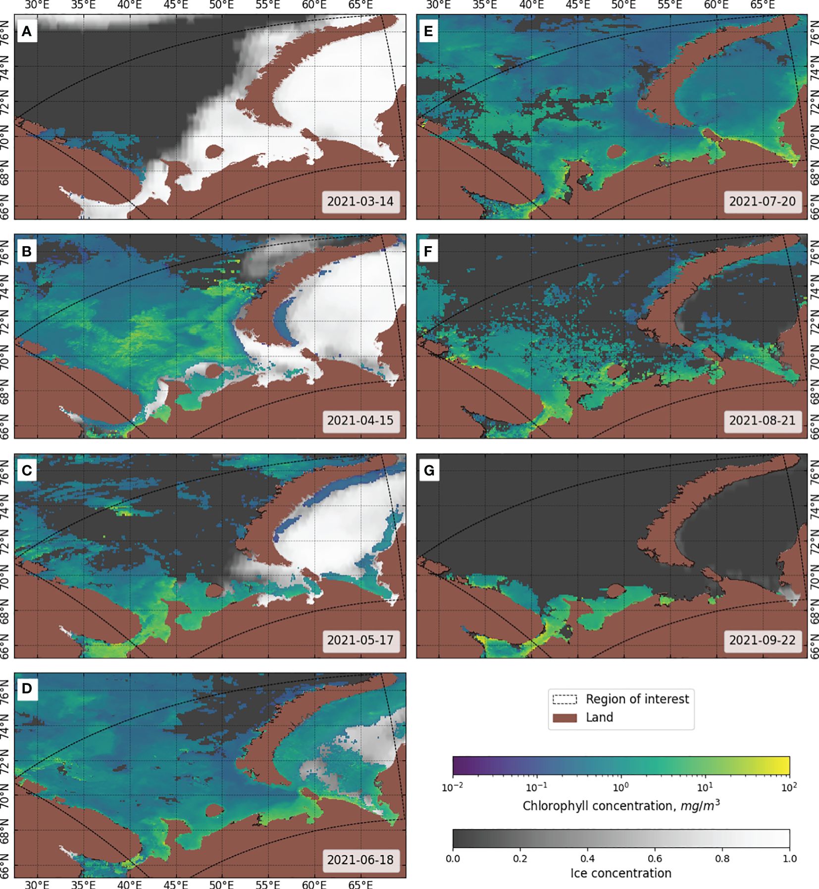
Figure 4 Examples of MODIS 8-day mean Chl-a and single-day ice concentration observations in the study area for the year 2021 in 32-day increments. (A) 14 March, (B) 15 April, (C) 17 May, (D) 18 June, (E) 20 July, (F) 21 August, (G) 22 September.

Figure 5

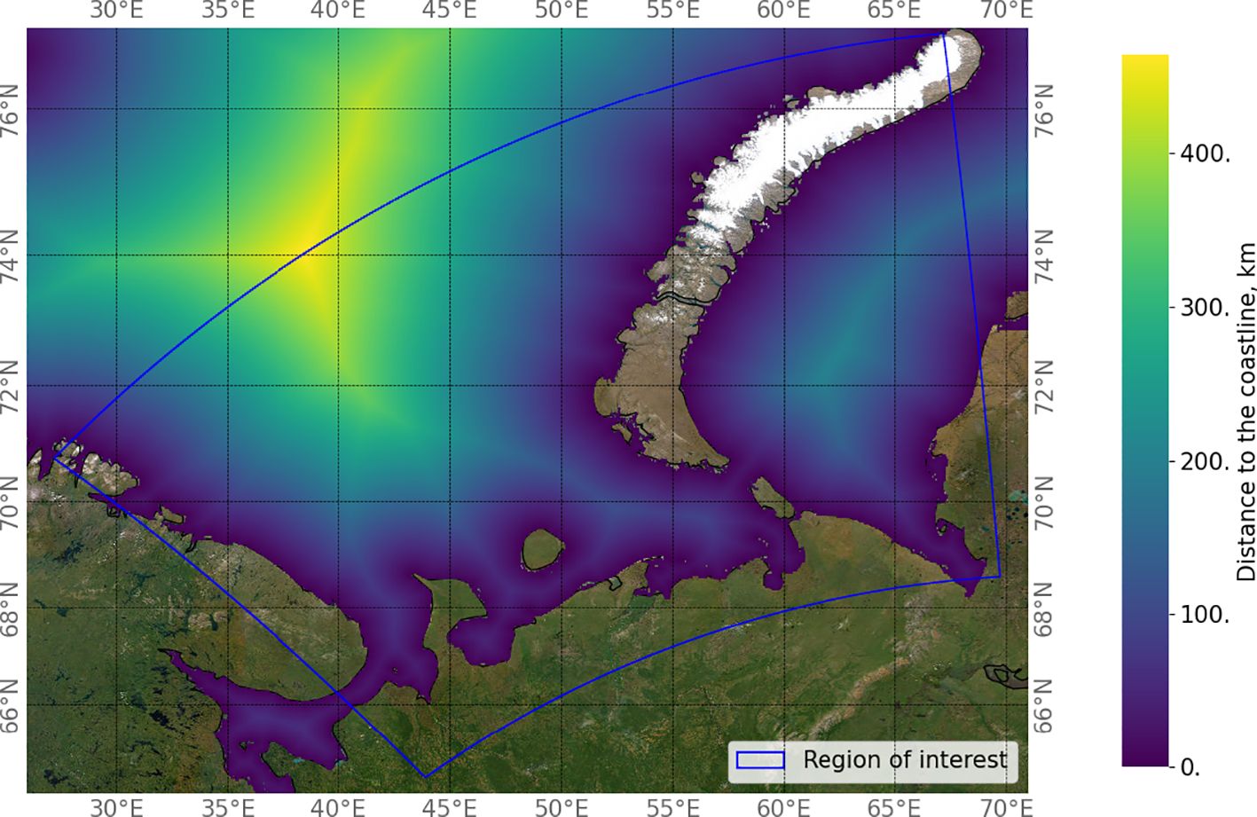
Figure 5 Shortest distance to the coastline in the region of interest.

In this paper, a split into training and test samples was performed to train and evaluate machine learning models using a dataset for each coordinate of the region of interest. The dataset is represented by 102 snapshots, each corresponding to a different 8-day interval and containing numerical values for spatially distributed variables at points in the region of interest, comprising over 130k unique coordinates (latitude and longitude pairs). Data for the time period from 1 January 2019 to 30 June 2022 were used to train the model, and data from 1 July 2022 to 31 December 2022 were used for testing. We have followed the common practice of choosing the test period for predictive models at the end of the time interval, which prevents data leakage from the future for estimating the model’s predictive ability for the new period. Figure 6 shows the distribution of chlorophyll concentration values for the interval from 0 to 10 mg/m³.

Figure 6

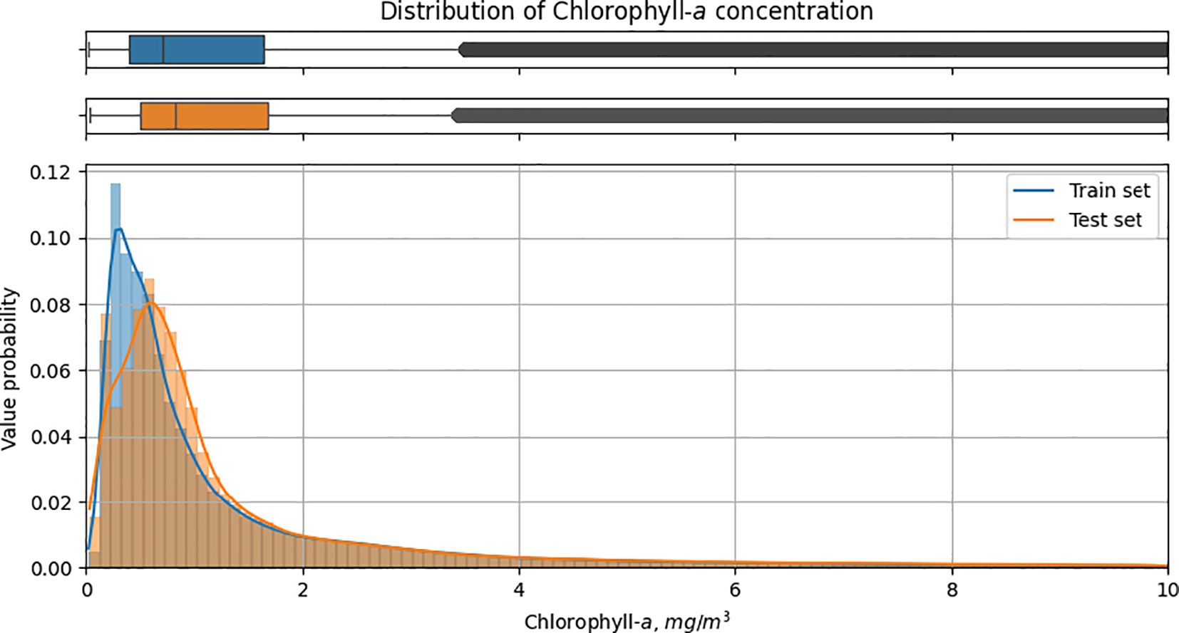
Figure 6 Distribution of chl-a concentration values for the interval from 0 to 10 mg/m³ in train and test sets.

2.4 Machine learning and deep learning methods

The paper compares the performance of classical machine learning algorithms and the neural network approach.

2.4.1 LightGBM

LightGBM’s (Ke et al., 2017) implementation of the gradient boosting decision tree method was used as the classical machine learning algorithm. One of the most important capabilities of LightGBM is its ability to handle missing values in features, both in the training period and in the prediction period. When Chl-a of preceding days is used as one of the input features for the model, missing data are inevitably observed for a large number of coordinates. Therefore, when using this feature, we excluded from training all coordinates where the preceding value is unknown. At the same time, when making predictions for the region of interest, we use all its coordinates regardless of the presence of gaps in the preceding values. In the case of the gradient boosting machine, if there are no gaps in the training data, the gaps in the test data follow the majority direction for the decision tree (the direction with the largest number of observations). The following parameters of the LightGBM model were used: number of boosted trees equal to 100, learning rate equal to 0.1, and tree depth without limit. An important parameter of the framework used is the “class weighting”, which allows us to perform a probability calibration of the model; it adjusts the weights inversely proportional to the frequencies of the target continuous values in the input data. The gradient boosting model was trained to make pixel-by-pixel predictions. The data were converted to a tabular format, where each row corresponds to the values of the features in a single coordinate.

2.4.2 Resnet-18

A neural network model based on the ResNet-18 (He et al., 2016) architecture was developed and trained using the PyTorch library. This architecture has proven to be effective for environmental spatial forecasting creation (Cheng et al., 2022; Shadrin et al., 2024). The aim of this study was to solve the regression problem. Therefore, the model was input with spatial data in the form of patches of 33 × 33 pixels, and the model was trained to predict the value of chlorophyll concentration in the center pixel of the patch. All values input to the model were scaled using min–max normalization. For land coordinates, feature values defined for sea coordinates only were set to −1. Gaps in the previous chlorophyll concentration values were filled by interpolation. Then, only those patches were selected for the model that contained at least one water pixel and had no gaps for any value. To improve the robustness of the model, instead of partitioning each file into patches with a fixed grid, new offsets were generated for each training epoch to slice the patches. The ResNet-18 model architecture was adapted to handle the input data, with the number of input channels equal to the number of features. An Adam optimizer with an initial learning rate of 10⁻³ and a step scheduler, which reduced the learning rate by a multiplier of 0.2 every 10 epochs, was chosen to optimize the learning process. The mean squared error was used as a loss function. The model training process was performed for 50 epochs with patch updates and batch size equal to 256.

2.5 Evaluation metrics

To assess the quality of model forecasts, a comparison is made between actual data and forecasted values. For regression tasks, the following set of metrics is often used: MAE (mean absolute error), RMSE (root mean square error), MAPE (mean absolute percentage error), and R² (coefficient of determination). All metrics were calculated in the per-pixel format. If ${\widehat{y}}_i$ is the predicted value of the ith pixel, $y_i$ is the corresponding true value and ${\overline{y}}_i$ is the arithmetic mean of all $y_i$, then RMSE (Equation 1), MAE (Equation 2), MAPE (Equation 3), and R² (Equation 4), estimated for n pixels, are determined as follows:

$\begin{array}{ll}RMSE(y,\widehat{y})=\sqrt{\frac{1}{n}{\displaystyle \sum _{i=1}^n{(y_i-{\widehat{y}}_i)}^2}}& (1)\end{array}$

$\begin{array}{ll}MAE(y,\widehat{y})=\frac{1}{n}{\displaystyle \sum _{i=1}^n|y_i-{\widehat{y}}_i|}& (2)\end{array}$

$\begin{array}{ll}MAPE(y,\widehat{y})=\frac{1}{n}{\displaystyle \sum _{i=1}^n\frac{\left|y_i-{\widehat{y}}_i\right|}{y_i}}& (3)\end{array}$

$\begin{array}{ll}{R}^2=1-\frac{{\displaystyle {\sum }_{i=1}^n{(y_i-{\widehat{y}}_i)}^2}}{{\displaystyle {\sum }_{i=1}^n{(y_i-{\overline{y}}_i)}^2}}& (4)\end{array}$

3 Results

3.1 Training of the models

The goal of the study is to develop an approach to forecast chl-a concentration for the next 8 days based on available atmospheric, oceanic, and remote sensing data. MODIS measurements of the chl-a concentration were selected as reference data for model development and its quality assessment. Moreover, MODIS data from the preceding period are used as features to forecast chl-a concentration for the succeeding days. The presence of dense cloud cover justifies the consideration of not only visible remote sensing measurements collected by the MODIS satellite but also data from NEMO and WRF models to generate additional features for analysis. These data include modeled measurements of atmospheric and oceanic systems for several upcoming days. The total number of features was 40. In addition to MODIS, WRF, and NEMO, an additional feature related to the distance to the coast and the day of the year is considered. The change in the quality of model performance when excluding some attributes from the training set, particularly the value of chlorophyll concentration for the previous period and the distance to the shore, was assessed.

Two machine learning approaches were employed to process the collected data. The first approach utilized a classical machine learning algorithm, LightGBM, which was applied to process individual pixels without considering their context. In contrast, the deep neural network approach incorporates the spatial distribution of neighboring pixels into consideration.

The change in the values of error and R² metric during Resnet-18 model training is presented in Figure 7. Loss and R² converge, and the fluctuations in their values are due to the fact that a new grid is generated at each epoch for training and validation to extract patches from the data snapshots. The R² value (0.687) of the validation measure is significantly higher than that of the test on the whole region (0.406) because the validation metric is calculated on a randomly selected set of patches sliced with a step equal to the patch size, while for the test, all possible patches are used with a step of 1 pixel.

Figure 7

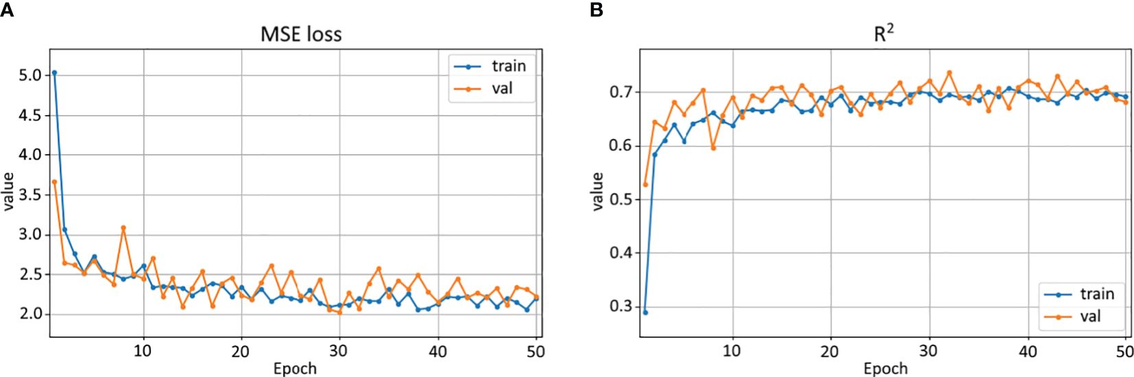
Figure 7 MSE loss and R² versus epoch during the Resnet-18 model training. (A) MSE loss, (B) R².

3.2 Assessing the quality of models

Experiments with different input features were conducted for these two machine learning models, and the resulting metrics are presented in Table 1 for the test dates. The median value serves as a baseline, representing the performance of a prediction strategy where all samples are assigned the median value of the chl-a concentration in the train set. As expected, this baseline approach yields relatively high errors across all metrics. A negative R² value of –0.191 indicates the complexity in the distribution of target variables.

Table 1

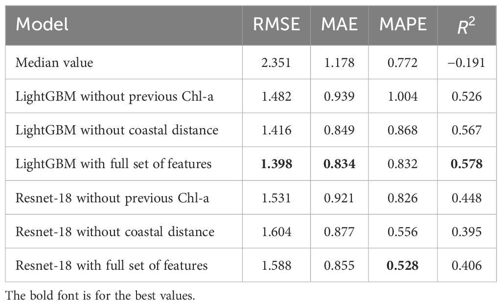
Table 1 Experimental results for the chl-a concentration estimation on the test subset using different models.

Using the full set of features in the LightGBM model gives the most favorable results, with the lowest RMSE equal to 1.398, MAE equal to 0.834, and the highest R² equal to 0.578, indicating superior predictive performance compared to other models. In particular, the Resnet-18 model with the full set of features shows competitive performance compared to its LightGBM counterpart. In particular, it achieves the lowest MAPE equal to 0.528, indicating its effectiveness in reducing prediction errors and maintaining consistency across different data points. Moreover, even the weakest of the presented deep learning models showed better MAPE values than any of the presented variations of classical machine learning models. The simultaneous deterioration of R² and improvement of MAPE when moving from classical learning models to deep learning models suggests that the model loses explanatory power but achieves greater predictive accuracy, which may indicate the greater practical utility of the model for making accurate predictions. For the LightGBM model, the standard deviations for all metrics were calculated from 20 runs of training the model with different random states. The following standard deviation values were obtained: σ(RMSE) = 8.2 × 10⁻³, σ(MAE) = 6.8 × 10⁻³, σ(MAPE) = 0.018, and σ(R²) = 4.9 × 10⁻³, which confirms the statistical significance of the results obtained. The achieved values of the R² metric are comparable to the values obtained for the northern marine regions by Zhang et al. (2023).

3.3 Feature importance analysis

We analyzed the feature importance for the classical machine learning model in the setup with all available features. The conducted study is intended to improve explainability of the achieved results and to help in further studies. Feature importance derived from LightGBM is shown in Figure 8. Latitude and longitude are among the most significant features. The reason is the strong correlation between distance to the coastal line and chl-a concentration. Generally, the higher chlorophyll concentration occurs near the particular regions of the shore. However, latitude and longitude are more informative features than just a coastal distance due to patterns in biochemical conditions associated with marine currents and other processes. U and V components of the wind speed at a height of 10 m also affect the model’s forecasting. It allows assessing the spread velocity and direction of flows in upcoming days. One of the most important attributes is atmospheric pressure, the influence of which on chlorophyll is complex. It can be assumed that changes in pressure lead to changes in weather conditions and illumination, which affect phytoplankton growth and plant photosynthesis. Nevertheless, the joint contribution of the all selected features is significant for the ultimate results.

Figure 8

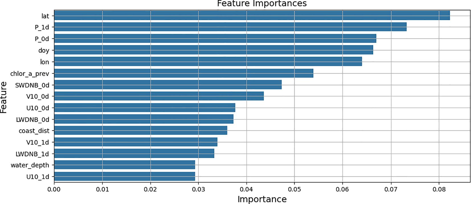
Figure 8 Feature importances (15 features with the highest importance values).

3.4 Visualization of the results

The visual assessment results for the best LightGBM and best Resnet-18 models are shown in Figures 9, 10, respectively. The results are presented for similar data to allow comparison of the results of the two approaches. The absolute error is calculated by subtracting the ground truth Chl-a values from the predicted Chl-a values.

Figure 9

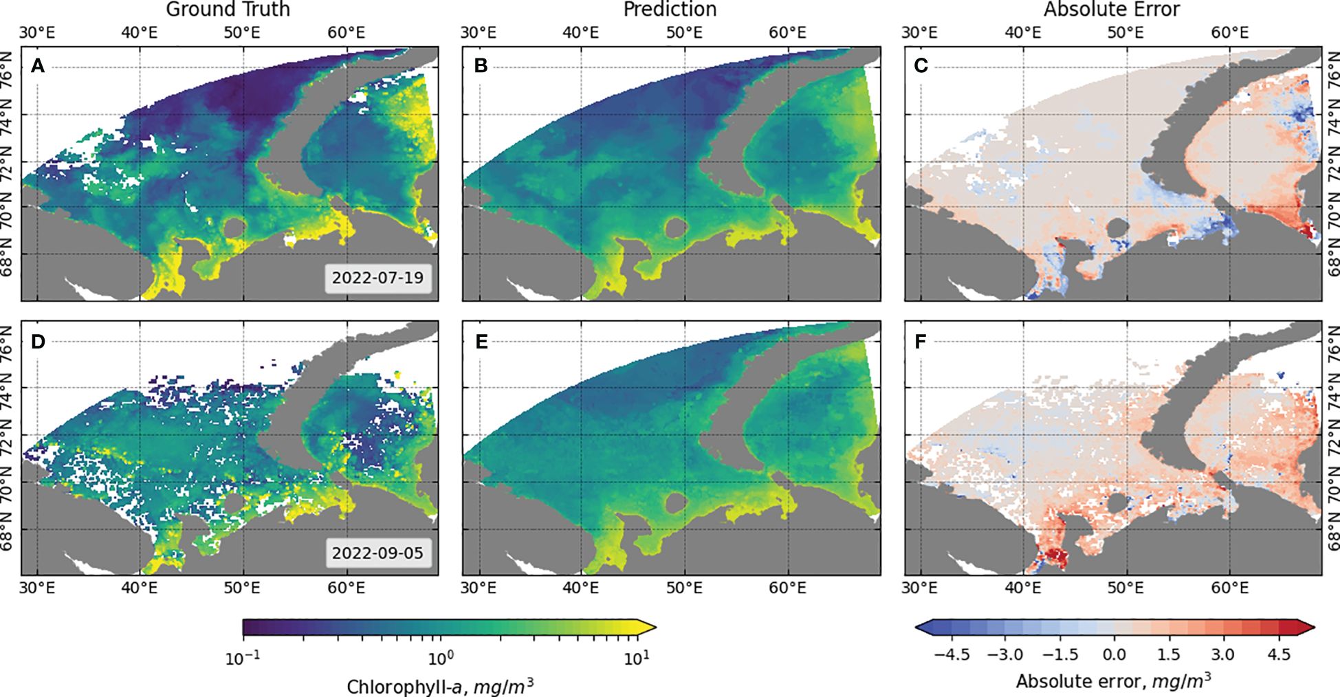
Figure 9 Comparison of ground truth and LightGBM model predicted values of Chl-a for individual snapshots from the data. (A) Ground truth, (B) prediction, and (C) absolute error for 8 days starting 19 July 2022, and (D) ground truth, (E) prediction, and (F) absolute error for 8 days starting 5 September 2022.

Figure 10

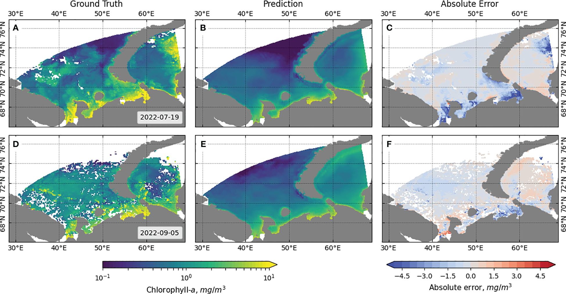
Figure 10 Comparison of ground truth and Resnet-18 model predicted values of Chl-a for individual snapshots from the data. (A) Ground truth, (B) prediction, and (C) absolute error for 8 days starting 19 July 2022, and (D) ground truth, (E) prediction, and (F) absolute error for 8 days starting 5 September 2022.

It can be observed that the ML-based model performs well in identifying clusters of points with high chlorophyll concentration, but at the same time, it tends to predict, on average, higher values than the actual values, especially in the coastal region. In contrast, the DL-based algorithm has a smaller error over a larger area of the region of interest and provides more accurate predictions for areas further from the coast, but misses areas of high concentration and predicts lower values than the actual values. The reduction in the number of points for which prediction is performed in the region of interest in the case of the DL model is due to the operation of the algorithm for selecting the patches fed to the model input: patches that do not contain gaps in the 33 × 33 square surrounding the pixel with the target Chl-a value are selected. On the border of this region, some pixels do not contain the values of NEMO variables.

4 Discussion

In the geo-spatial tasks, the spatial context usually plays a vital role (Illarionova et al., 2021). Therefore, we compared two approaches that involve or ignore it. The main advantage of the classical machine learning model is its faster training and inference process in comparison with deep neural network. Moreover, the shorter amount of tunable parameters makes it easier to develop an ML-based approach. Although DL-based solutions require a finer adjustment, in various geo-spatial tasks, they have proven to outperform the classical approaches.

Despite the continuous improvement of MODIS products and remote sensing tools in general, there are uncertainties and biases in the data acquisition process. The quality is strongly influenced by the angle of coverage and the angle of incident light (Barnes and Hu, 2016) and other factors. In addition, as the final chlorophyll concentration values are determined from an empirical relationship, some additional discrepancies are possible. It has been repeatedly shown that the credibility of MODIS chlorophyll concentration products in offshore waters is poor and significantly overestimated (Darecki and Stramski, 2004; Harshada et al., 2021). Therefore, the error of remotely sensed chlorophyll concentration data in coastal waters is very large and, in fact, MODIS Chl-a for these regions characterizes the concentration of terrestrial suspended particulates rather than the true chlorophyll concentration. Alternative data sources can complement and improve the accuracy of satellite-derived chlorophyll estimates. In situ measurements from oceanographic buoys, research vessels, and autonomous underwater vehicles provide direct observations of chlorophyll concentration at specific locations. In addition, high-resolution models that integrate physical and biological processes can simulate chlorophyll distribution based on environmental parameters.

Our study presents an approach to predict chlorophyll concentration in marine waters using a model based on ocean and atmospheric dynamics data. A major advantage of this approach is that, although the model is trained on satellite-derived chlorophyll data, the input parameters of the model are not sensitive to the illumination conditions of the input data. This allows us to continue forecasting in conditions where satellite data would have limited availability due to cloud cover or short day length in winter. At the same time, the approach presented can be used to create a model trained on more accurate data.

There are several considerations when evaluating the generalization ability of the machine learning model used. First, machine learning models are expected to generalize effectively as the size of the model and training dataset increases. The NEMO ocean model at high spatial resolution (approximately 3 km) presents significant computational challenges when applied to extensive regions such as the entire Arctic. These challenges arise from mesoscale instabilities and numerical drift of WRF and NEMO models from reference values in the middle of the study area. The primary issue is the need to validate and consistently run the ocean model to avoid significant deviations from in situ and satellite data. To address model drift, statistical corrections such as nudging are required. Similar procedures are required for the atmospheric model, including ensuring model stability based on initial and boundary conditions, and maintaining physical consistency with observations within the study area.

In addition to the challenges associated with numerical modeling for creating large datasets, it is important to discuss the generalizability of the machine learning model to new geographical regions. A common approach for spatiotemporal analysis involves training the model on data from one specific region and then testing it on data from another region. Conducting such experiments can provide further insight into the model’s ability to adapt to new geographical regions. A promising avenue is to explore the optimal amount of additional data required to support such adaptation. However, these experiments were beyond the scope of the current research, which primarily focused on temporal robustness (forecasting for new dates for the same region) rather than spatial robustness (forecasting for the same dates for different regions) of the developed algorithm. Future studies could address these limitations to explore the generalizability of the approach in different geographical contexts, considering both spatial and temporal components.

5 Conclusion

In this study, we explored and developed a machine learning-based solution for predicting chl-a concentration in northern marine regions. This environmental parameter is crucial for a comprehensive understanding of the interactions between the atmosphere and ocean. Traditional methods rely mostly on local measurements and may not be suitable for spatiotemporal analysis of vast regions. Therefore, we integrated NEMO and WRF modeling data into our solution, which proved to be effective for reconstructing satellite-based chlorophyll-a measurements when spectral remote sensing is limited due to polar night or cloud cover.

The Barents Sea was selected as the study area due to its unique environmental properties, particularly the presence of warm Atlantic water leading to largely ice-free conditions throughout the year. Using the collected dataset for this region, we conducted a series of experiments to determine the most relevant approach for estimating chl-a concentration. The LightGBM model achieved the highest accuracy with an R² value of 0.578. However, in terms of the MAPE metric, the Resnet-18 model outperformed the LightGBM with a value of 0.527 (compared to 0.831 for LightGBM).

Among the most important features for concentration prediction were longitude and latitude, wind speed, and atmospheric pressure. In future studies, this proposed approach can be expanded to include other northern waters and incorporate additional biogeochemical characteristics. Overall, estimating chl-a concentrations based on spatiotemporal modeling can serve as a reliable indicator of ecological conditions in vast regions.

Data availability statement

The raw data supporting the conclusions of this article will be made available by the authors, without undue reservation.

Author contributions

MA: Conceptualization, Data curation, Formal analysis, Investigation, Methodology, Software, Visualization, Writing – original draft. SI: Conceptualization, Formal analysis, Investigation, Methodology, Supervision, Writing – original draft. DS: Conceptualization, Formal analysis, Supervision, Writing – original draft. VI: Data curation, Formal analysis, Writing – original draft. VV: Data curation, Formal analysis, Supervision, Writing – original draft. EB: Conceptualization, Funding acquisition, Project administration, Supervision, Validation, Writing – original draft.

Funding

The author(s) declare financial support was received for the research, authorship, and/or publication of this article. The work was supported by the Analytical center under the RF Government (subsidy agreement 000000D730321P5Q0002, Grant No. 70-2021-00145 02.11.2021).

Conflict of interest

The authors declare that the research was conducted in the absence of any commercial or financial relationships that could be construed as a potential conflict of interest.

The author(s) declared that they were an editorial board member of Frontiers, at the time of submission. This had no impact on the peer review process and the final decision.

Publisher’s note

All claims expressed in this article are solely those of the authors and do not necessarily represent those of their affiliated organizations, or those of the publisher, the editors and the reviewers. Any product that may be evaluated in this article, or claim that may be made by its manufacturer, is not guaranteed or endorsed by the publisher.

References

Alvarez-Fernandez S., Riegman R. (2014). Chlorophyll in north sea coastal and offshore waters does not reflect long term trends of phytoplankton biomass. J. Sea Res. 91, 35–44. doi: 10.1016/j.seares.2014.04.005

CrossRef Full Text | Google Scholar

Alvera-Azcárate A., van der Zande D., Barth A., Troupin C., Martin S., Beckers J.-M. (2021). Analysis of 23 years of daily cloud-free chlorophyll and suspended particulate matter in the greater north sea. Front. Mar. Sci. 8. doi: 10.3389/fmars.2021.707632

CrossRef Full Text | Google Scholar

Anderson D. M., Glibert P. M., Burkholder J. M. (2002). Harmful algal blooms and eutrophication: nutrient sources, composition, and consequences. Estuaries 25, 704–726. doi: 10.1007/BF02804901

CrossRef Full Text | Google Scholar

Barnes B. B., Hu C. (2016). Dependence of satellite ocean color data products on viewing angles: A comparison between seawifs, modis, and viirs. Remote Sens. Environ. 175, 120–129. doi: 10.1016/j.rse.2015.12.048

CrossRef Full Text | Google Scholar

Barnier B., Blaker A., Biastoch A., Böning C. W., Coward A., Deshayes J., et al. (2015). Drakkar: Developing high resolution ocean components for european earth system models. Clivar Exchanges 65, 18–21.

Google Scholar

Bierman P., Lewis M., Ostendorf B., Tanner J. (2011). A review of methods for analysing spatial and temporal patterns in coastal water quality. Ecol. Indic. 11, 103–114. doi: 10.1016/j.ecolind.2009.11.001

CrossRef Full Text | Google Scholar

Cen H., Jiang J., Han G., Lin X., Liu Y., Jia X., et al. (2022). Applying deep learning in the prediction of chlorophyll-a in the east China sea. Remote Sens. 14, 5461. doi: 10.3390/rs14215461

CrossRef Full Text | Google Scholar

Cheng X., Zhang W., Wenzel A., Chen J. (2022). Stacked resnet-lstm and coral model for multi-site air quality prediction. Neural Computing Appl. 34, 13849–13866. doi: 10.1007/s00521-022-07175-8

CrossRef Full Text | Google Scholar

Cho H., Park H. (2019). “Merged-lstm and multistep prediction of daily chlorophyll-a concentration for algal bloom forecast,” in IOP) Conference Series: Earth and Environmental Science, (Bristol, England: IOP). Vol. 351. 012020. doi: 10.1088/1755-1315/351/1/012020

CrossRef Full Text | Google Scholar

Darecki M., Stramski D. (2004). An evaluation of modis and seawifs bio-optical algorithms in the baltic sea. Remote Sens. Environ. 89, 326–350. doi: 10.1016/j.rse.2003.10.012

CrossRef Full Text | Google Scholar

Desmit X., Nohe A., Borges A. V., Prins T., De Cauwer K., Lagring R., et al. (2020). Changes in chlorophyll concentration and phenology in the north sea in relation to de-eutrophication and sea surface warming. Limnology Oceanography 65, 828–847. doi: 10.1002/lno.11351

CrossRef Full Text | Google Scholar

Dvoretsky V. G., Vodopianova V. V., Bulavina A. S. (2023). Effects of climate change on chlorophyll a in the barents sea: A long-term assessment. Biology 12, 119. doi: 10.3390/biology12010119

PubMed Abstract | CrossRef Full Text | Google Scholar

European Union-Copernicus Marine Service (2016). Global ocean 1/12ř physics analysis and forecast updated daily. doi: 10.48670/MOI-00016

CrossRef Full Text | Google Scholar

Fetterer F., Knowles K., Meier W., Savoie M., K W. A. (2017). Sea ice index, version 3. doi: 10.7265/N5K072F8

CrossRef Full Text | Google Scholar

Guo Y., Chen S., Li X., Cunha M., Jayavelu S., Cammarano D., et al. (2022). Machine learning-based approaches for predicting spad values of maize using multi-spectral images. Remote Sens. 14, 1337. doi: 10.3390/rs14061337

CrossRef Full Text | Google Scholar

Guo Y., Fu Y., Hao F., Zhang X., Wu W., Jin X., et al. (2021). Integrated phenology and climate in rice yields prediction using machine learning methods. Ecol. Indic. 120, 106935. doi: 10.1016/j.ecolind.2020.106935

CrossRef Full Text | Google Scholar

Guo Y., Xiao Y., Hao F., Zhang X., Chen J., de Beurs K., et al. (2023). Comparison of different machine learning algorithms for predicting maize grain yield using uav-based hyperspectral images. Int. J. Appl. Earth Observation Geoinformation 124, 103528. doi: 10.1016/j.jag.2023.103528

CrossRef Full Text | Google Scholar

Harshada D., Raman M., Jayappa K. (2021). Evaluation of the operational chlorophyll-a product from global ocean colour sensors in the coastal waters, south-eastern arabian sea. Egyptian J. Remote Sens. Space Sci. 24, 769–786. doi: 10.1016/j.ejrs.2021.09.005

CrossRef Full Text | Google Scholar

He K., Zhang X., Ren S., Sun J. (2016). “Deep residual learning for image recognition,” in 2016 IEEE Conference on Computer Vision and Pattern Recognition (CVPR). (New York City, USA: IEEE) 770–778. doi: 10.1109/CVPR.2016.90

CrossRef Full Text | Google Scholar

Hemmings J., Challenor P. G., Yool A. (2015). Mechanistic site-based emulation of a global ocean biogeochemical model (medusa 1.0) for parametric analysis and calibration: an application of the marine model optimization testbed (marmot 1.1). Geoscientific Model. Dev. 8, 697–731. doi: 10.5194/gmd-8-697-2015

CrossRef Full Text | Google Scholar

Hill V., Light B., Steele M., Sybrandy A. L. (2022). Contrasting sea-ice algae blooms in a changing arctic documented by autonomous drifting buoys. J. Geophysical Research: Oceans 127, , e2021JC017848. doi: 10.1029/2021jc017848

CrossRef Full Text | Google Scholar

Hu C., Feng L., Guan Q. (2021). A machine learning approach to estimate surface chlorophyll a concentrations in global oceans from satellite measurements. IEEE Trans. Geosci. Remote Sens. 59, 4590–4607. doi: 10.1109/TGRS.2020.3016473

CrossRef Full Text | Google Scholar

Hu C., Feng L., Lee Z., Franz B. A., Bailey S. W., Werdell P. J., et al. (2019). Improving satellite global chlorophyll a data products through algorithm refinement and data recovery. J. Geophysical Research: Oceans 124, 1524–1543. doi: 10.1029/2019JC014941

CrossRef Full Text | Google Scholar

Illarionova S., Nesteruk S., Shadrin D., Ignatiev V., Pukalchik M., Oseledets I. (2021). “Object-based augmentation for building semantic segmentation: Ventura and santa rosa case study,” in Proceedings of the IEEE/CVF International Conference on Computer Vision. New York City, USA: IEEE 1659–1668.

Google Scholar

Illarionova S., Shadrin D., Tregubova P., Ignatiev V., Efimov A., Oseledets I., et al. (2022). A survey of computer vision techniques for forest characterization and carbon monitoring tasks. Remote Sens. 14, 5861. doi: 10.3390/rs14225861

CrossRef Full Text | Google Scholar

Ke G., Meng Q., Finley T., Wang T., Chen W., Ma W., et al. (2017). “Lightgbm: A highly efficient gradient boosting decision tree,” in Advances in neural information processing systems, vol. 30 . Eds. Guyon I., Luxburg U. V., Bengio S., Wallach H., Fergus R., Vishwanathan S., Garnett R. (Curran Associates, Inc, New York City, USA).

Google Scholar

Madec G., Bourdallé-Badie R., Bouttier P.-A., Bricaud C., Bruciaferri D., Calvert D., et al. (2017). Nemo ocean engine. France: Notes du Pôle de modélisation de l'Institut Pierre-Simon Laplace.

Google Scholar

Martinez E., Gorgues T., Lengaigne M., Fontana C., Sauzède R., Menkes C., et al. (2020). Reconstructing global chlorophyll-a variations using a non-linear statistical approach. Front. Mar. Sci. 7. doi: 10.3389/fmars.2020.00464

CrossRef Full Text | Google Scholar

NASA’s Ocean Biology Processing Group (2024). Near-surface concentration of chlorophyll-a. USA: NASA Goddard Space Flight Center. Available at: https://oceandata.sci.gsfc.nasa.gov/directdataaccess/Level-3%20Mapped/Aqua-MODIS.

Google Scholar

National Centers for Environmental Prediction, National Weather Service, NOAA, U.S. Department of Commerce (2015). Ncep gfs 0.25 degree global forecast grids historical archive. Boulder, Colorado, USA: Research Data Archive at the National Center for Atmospheric Research, Computational and Information Systems Laboratory. doi: 10.5065/D65D8PWK

CrossRef Full Text | Google Scholar

O’Reilly J. E., Werdell P. J. (2019). Chlorophyll algorithms for ocean color sensors - oc4, oc5 & oc6. Remote Sens. Environ. 229, 32–47. doi: 10.1016/j.rse.2019.04.021

PubMed Abstract | CrossRef Full Text | Google Scholar

Pereira H., Picado A., Sousa M. C., Brito A. C., Biguino B., Carvalho D., et al. (2023). Effects of climate change on aquaculture site selection at a temperate estuarine system. Sci. Total Environ. 888, 164250. doi: 10.1016/j.scitotenv.2023.164250

PubMed Abstract | CrossRef Full Text | Google Scholar

Rajaee T., Boroumand A. (2015). Forecasting of chlorophyll-a concentrations in south san francisco bay using five different models. Appl. Ocean Res. 53, 208–217. doi: 10.1016/j.apor.2015.09.001

CrossRef Full Text | Google Scholar

Rieck J. K., Böning C. W., Greatbatch R. J., Scheinert M. (2015). Seasonal variability of eddy kinetic energy in a global high-resolution ocean model. Geophysical Res. Lett. 42, 9379–9386. doi: 10.1002/2015GL066152

CrossRef Full Text | Google Scholar

Rousseaux C. S., Gregg W. W. (2017). Forecasting ocean chlorophyll in the equatorial pacific. Front. Mar. Sci. 4. doi: 10.3389/fmars.2017.00236

CrossRef Full Text | Google Scholar

Schalles J. F. (2006). Optical remote sensing techniques to estimate phytoplankton Chlorophyll A concentrations in coastal (Dordrecht: Springer Netherlands), 27–79. doi: 10.1007/1-4020-3968-9_3

CrossRef Full Text | Google Scholar

Shadrin D., Illarionova S., Gubanov F., Evteeva K., Mironenko M., Levchunets I., et al. (2024). Wildfire spreading prediction using multimodal data and deep neural network approach. Sci. Rep. 14, 2606. doi: 10.1038/s41598-024-52821-x

PubMed Abstract | CrossRef Full Text | Google Scholar

Shamshirband S., Jafari Nodoushan E., Adolf J. E., Abdul Manaf A., Mosavi A., Chau K.-w. (2019). Ensemble models with uncertainty analysis for multi-day ahead forecasting of chlorophyll a concentration in coastal waters. Eng. Appl. Comput. Fluid Mechanics 13, 91–101. doi: 10.1080/19942060.2018.1553742

CrossRef Full Text | Google Scholar

Skamarock W. C., Klemp J. B., Dudhia J., Gill D. O., Liu Z., Berner J., et al. (2019). A description of the advanced research wrf version 4. NCAR tech. note ncar/tn-556+ str 145. doi: 10.5065/1dfh-6p97

CrossRef Full Text | Google Scholar

Smedsrud L. H., Esau I., Ingvaldsen R. B., Eldevik T., Haugan P. M., Li C., et al. (2013). The role of the barents sea in the arctic climate system. Rev. Geophysics 51, 415–449. doi: 10.1002/rog.20017

CrossRef Full Text | Google Scholar

Van Klompenburg T., Kassahun A., Catal C. (2020). Crop yield prediction using machine learning: A systematic literature review. Comput. Electron. Agric. 177, 105709. doi: 10.1016/j.compag.2020.105709

CrossRef Full Text | Google Scholar

Verezemskaya P., Barnier B., Gulev S. K., Gladyshev S., Molines J.-M., Gladyshev V., et al. (2021). Assessing eddying (1/12) ocean reanalysis glorys12 using the 14-yr instrumental record from 59.5 n section in the atlantic. J. Geophysical Research: Oceans 126, e2020JC016317. doi: 10.1029/2020JC016317

CrossRef Full Text | Google Scholar

Ye H., Tang S., Yang C. (2021). Deep learning for chlorophyll-a concentration retrieval: A case study for the pearl river estuary. Remote Sens. 13, 3717. doi: 10.3390/rs13183717

CrossRef Full Text | Google Scholar

Zhang Z., Chen P., Zhong C., Xie C., Sun M., Zhang S., et al. (2023). Chlorophyll and poc in polar regions derived from spaceborne lidar. Front. Mar. Sci. 10. doi: 10.3389/fmars.2023.1050087

CrossRef Full Text | Google Scholar