Regional tidal modeling on the European coast using tide gauges and satellite altimetry

The study investigates sea-level measurements along the coastal area of Europe for the 60-year (1961–2020) time span. Linear and quadratic modeling of tide gauge measurements showed an almost positive rate of trend of sea-level rise (0.09 to 3.6 mm/yr) and low acceleration (−0.05 to 0.40 mm/yr²). A least-squares harmonic estimation tidal modeling was carried out to estimate frequency (cycles per day) for a certain period. The smaller and higher tidal frequencies of these stations indicate their stability in terms of their surface variation. We used the 1993–2020 satellite altimetry data from the nearest grid points of the tide gauge station. The correlation coefficient between observed and satellite altimetry (lowest 0.53 and highest 0.93) varies at each station. This happens because of many factors that can affect the large difference in the sea-level trend between the satellite-derived and tide gauge results. Finally, to implement a global reference system for physical heights, the offshore topographic slope direction and slope range with contour spacing from the sea to the associated coastline were analyzed using bathymetry data. The abrupt change in slope from the coastline toward the sea can be seen toward the east, west, and southeast on the European coast. This is also an important factor that affects the variation of sea level.

1 Introduction

The rise of sea levels worldwide in coastal areas can lead to mega floods (Buchanan et al., 2017; Taherkhani et al., 2020; Ansari, 2022; Ezer, 2023). This kind of sea-level rise is a global issue, which threatens coastal human population and infrastructure. The cost of socioeconomic losses also includes degradation of soil and water quality, agriculture source reduction, and damage to infrastructure (Ghazali et al., 2018; Balogun and Adebisi, 2021). Therefore, the prediction of sea-level variation as accurately as possible is important for the economic growth of communities belonging to the coastal region.

Tide gauge data play an important role and provide a long-term record of sea level at a temporal scale at the installation location. Although these stations can provide data at a very precise level, they are sparse due to the unequal distribution and relative measurement concerning the solid Earth (Cipollini et al., 2017). Tide gauge measurements are affected because of the subsidence of land and the rise in an estimation requirement of vertical land motion to understand the change in absolute sea level (Holgate et al., 2013; Ansari and Bae, 2021; Balogun and Adebisi, 2021). The variation of sea level of ~10–20 cm on a large global scale occurred because of a tectonic process in the last 100 Ma (Haq and Schutter, 2008; Müller et al., 2008; Miller et al., 2011; Mey et al., 2016; Young et al., 2022). Approximately 26,500 years ago, one of the lowest sea levels existed during the last glacial maximum (He et al., 2022). The global rise of sea level exceeded 122 cm, which is greater than the present-day estimation (Lambeck, 2014). Scientists noticed rapid variation in mean sea level in the last 200 years or so since the industrial era started. This is presumably related to greenhouse gas emissions (Shaw and Mukherjee, 2022). The rise of sea level and expansion of water occurred because of ocean/global warming (He et al., 2022). The glaciers of mountains are melting due to an increase in air temperature, which contributes to the rising of sea level with the freshwater inputs in the oceans.

The sea-level observations in coastal areas have been monitored by a tide gauge network for decades. Tide prediction, port operation, and datum definition are the great motivations behind establishing this network. Moreover, change in sea level at different temporal and spatial scales is to be understood by the researchers working in the fields of oceanography, geodesy, seismology, metrology, and hydrology. In addition, sea-level rise adversely affects hydrocarbon production from offshore areas. Therefore, the study of sea-level rise will have a far-reaching implication in petroleum production studies. The tide gauge observations are biased by regional processes that can be linear or non-linear in the decades of timescale. The glacial isostatic adjustment and accumulation of interseismic tectonic strain are the part of linear process, while non-linear includes earthquake or their post-seismic relaxation (Cazenave and Nerem, 2004; Emery and Aubrey, 2012). To understand these, it is necessary to consider high-quality data and correct the modeling process for sea-level analysis (Zhao et al., 2019; Ansari et al., 2020).

Although the mean sea-level trend with a timescale of long-term data has been well investigated, very few address the issue of sea-level acceleration in detail (Table 1). In this study, we investigated sea-level variation from 1961 to 2020 along ~68,000-km-long European coast by applying observations from the Permanent Service for Mean Sea Level (PSMSL; www.psmsl.org, Figure 1). The study area includes the coastlines of Finland, Sweden, Norway, Iceland, England, the Netherlands, France, Spain, Portugal, Italy, Greece, western Turkey, and Georgia. The main objective of this study is to examine the long-term trend of relative sea-level change in the north, south, and west European coasts at a regional scale.

Table 1

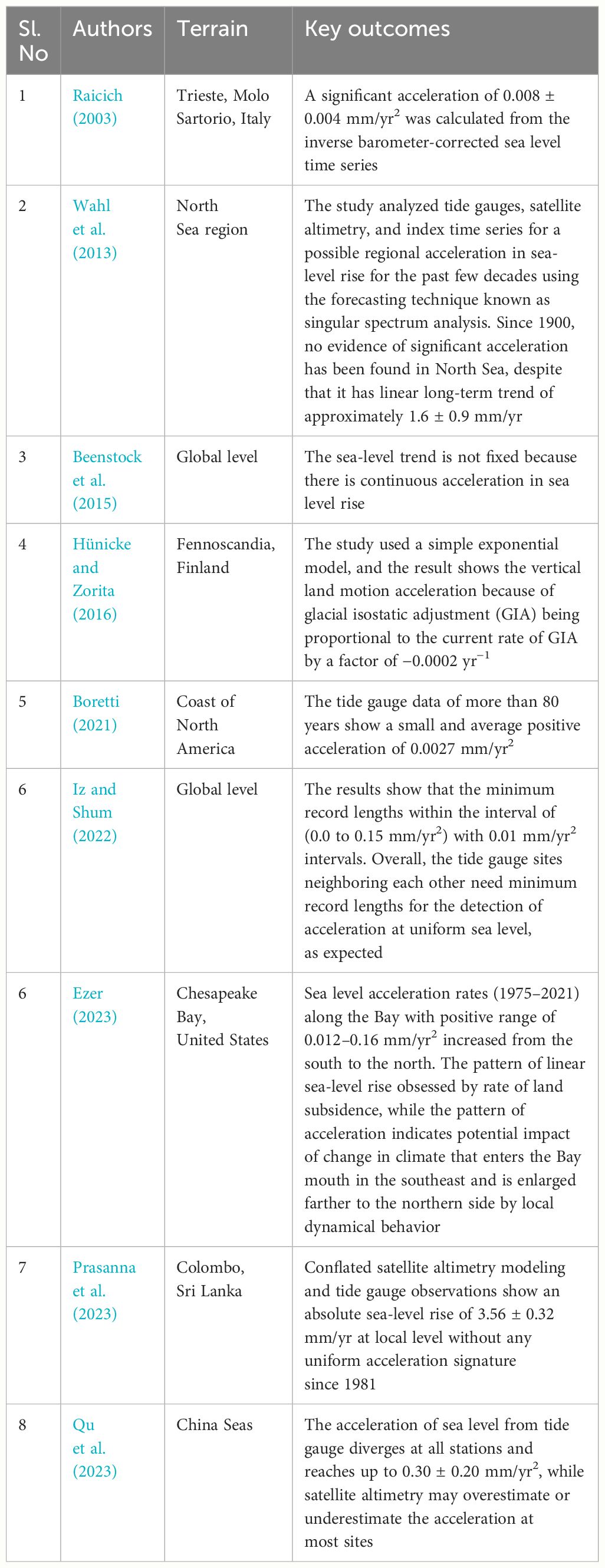
Table 1 Review of studies that used rate of acceleration of tide gauge measurements.

Figure 1

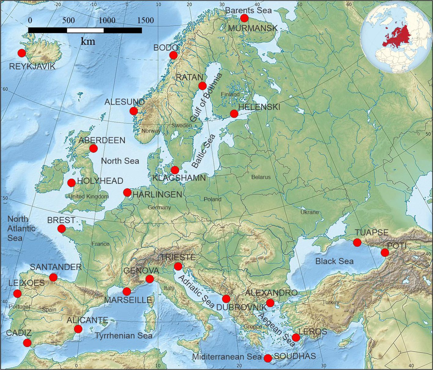
Figure 1 Location of the 24 selected tide gauge stations on European coast for the present study. The Permanent Service for Mean Sea Level (PSMSL) observation along the coastal area has been studied during 1961–2020 A.D. and satellite altimetry data during 1993–2020. No data are available before 1993.

PSMSL data provide monthly and annual records, in which the former data look more complete than the latter one. This is because annual records only can be used when 11 or 12 months of complete data are available. Hence, we selected only monthly data for the current study and focused on updated sea-level activities from 1961 to 2020. We used minimum records of the required length to detect the potential of uniform acceleration using quadratic modeling. The global tide gauge records measured at relative sea level oscillate with many periodicities. These important periodicities because of the oscillating behavior in the absence of major gaps or any perturbing events can be investigated using the relative sea-level data for >60 years or up to quasi 60 years (Parker, 2016). The general subsidence or uplift, any additional change in height, and vertical tide gauge velocities generate top-down (periodic) variation in the relative sea level. In the current study, to determine the effects periodically on sea-level measurements, we used the harmonic analysis (HA) method and prediction with least-squares estimation (Section 2). This periodic approach effectively detects and separates the low-frequency variation of sea level from tide gauge records and eliminates their confounding effects during the detection of sea-level acceleration.

It is more challenging to measure regional sea level within a smaller area compared to computing global sea level. It happens because ocean variability is generally larger on regional scales due to redistribution effects like wind (Breili et al., 2017). Here, the redistribution effect of wind refers to the presence and deployment of wind. Furthermore, altimetry measurement at the regional level is more sensitive regarding errors, often negligible when estimating the global average. This is possible because of ocean tide model error, orbital error, and the corrections in the sea state (Beckley et al., 2007). The satellite altimetry system used several satellites and improved the technique of sea-level monitoring at global sea-level changes since 1993. This is a very good technique for understanding the influence of water surface, real-time marine development, and the effect of local sea level (Araújo, 2022). Satellite altimetry is the main technique for measuring and mapping of topography of the sea surface and changes in sea level over the past 25 years. In the current study, gridded daily sea-level data were used, and an analysis with tide gauge observations was carried out. The satellite altimetry data from the European coast were collected from Global Ocean Gridded L4 Sea Surface Heights and Derived Variables Reprocessed Copernicus Climate Change Service (von Schuckmann et al., 2021; C3S, 2023). In the current study, the multi-mission satellite altimetry data were utilized to examine the absolute sea level variability at an absolute level on the European coast covering (20°N to 80°N and 10°W to 50°E) January 1993 to December 2020.

The global reference system implementation for physical heights of the International Height Reference System (IHRS) is a big task and needs wide scientific community support. The curves and depths of lower-level terrain are referred to as bathymetry in a wide sense. Generally, the digital bathymetric model (DBM) is used to determine marine topography for small areas (e.g., Klenke and Schenke, 2002; Hell, 2011). Prediction of bathymetry is a standard method in ocean mapping at regional and global scales (e.g., Amante and Eakins, 2008). With the first launch of the Seasat mission in 1978 by the USA, sea surface height undulations caused by the gravimetric method effects of underwater topography with satellite-based timers initiated have been remotely measured (Born et al., 1979). The development of multi-beam echo sounders in recent decades has greatly improved the efficiency, accuracy, and spatial resolution of mapping the shoreline and the ocean floor topography. The bathymetric dataset is based on the General Bathymetric Chart of the Oceans (GEBCO) global bathymetric grids developed in 2019 through The Nippon Foundation-GEBCO Seabed 2030 Project. It is a collaboration between the Nippon Foundation (Japan) and the GEBCO. In April 2023, the GEBCO_2023 Grid was made available. It offers elevation data in meters for the entire world in a grid with 15-arc-second intervals. With 43,200 rows and 86,400 columns, it has 3,732,480,000 data points worldwide. The elevations in meters at the center of grid cells are referenced by the data values, which are pixel-center registered (Internet ref-2). Toolbox plugin is used to find the slope direction and the amount. Contours of 100-m spacing are generated from the 3D data to generate the continental shelf-to-slope pattern. In the current study, the offshore topographic slope direction and slope ranges with contour spacing from the sea to the coastline associated with the study region are specified.

The results and discussion of the present study such as linear and quadratic, modeling of tide gauge using the 1961–2020 data, HA, and satellite altimetry analysis of the 1993–2020 data along with the bathymetric detail are explained in Section 3.

2 Tide gauge modeling

The slope of sea-level rise and its acceleration are studied using linear and quadratic fitting of long-term measurements. Suppose the given time series of sea-level measurement is given by S_t at a time t. The slope can be estimated by a linear fit (Parker, 2018):

$\begin{array}{ll}{S}_t=at+b& (1)\end{array}$

Constants a and b are applied to understand the slope average sea level during the period of observation. This is a classic approach that needs long-term recorded data (60 years in this study) to avoid the multi-decadal oscillation from peak to valley (Parker et al., 2013). For acceleration of sea-level rise, we need to fit the data in a quadratic form:

$\begin{array}{ll}{S}_t=\frac{1}{2}c{t}^2+dt+e& (2)\end{array}$

Here, c, d, and e are constants, with c representing the acceleration. This quadratic fitting is also known as parabolic fitting and allows estimating the acceleration of sea level in a certain period. Although such an analysis can provide the average acceleration of the tide gauge, only the second-order coefficient is not perfectly sufficient to understand the periodic variation. Therefore, a more complicated analysis is required to understand the sea-level changes. Thus, we used the least-squares harmonic estimation based on the principle of the HA method to determine the periodic effect on sea-level measurements. The functional model using tidal components has been developed as per Equation 3, known as frequencies on the sea-level data (Horn, 1960).

$\begin{array}{ll}h(t)=Ho+{\displaystyle \sum _{i=1}^k({\text{A}}_i\cos {\omega }_{i}t+B_i\sin {\omega }_{i}t)}& (3)\end{array}$

Here, h(t) indicates sea level tide gauge height at instant time with the respective predefined datum; Ho indicates height of mean sea level at time t; A_i and B_i are Fourier coefficients, which vary from 1 to some finite number k; ω_i indicates angular frequency. To determine the tidal component, a functional model by the least-squares method can be stated by Equation 4 (Erkoç and Doğan, 2022):

$\begin{array}{ll}l=Ax+\varepsilon with\varepsilon \approx (0,{\sigma }_0^2{P}^{-1})& (4)\end{array}$

$\begin{array}{ll}\left[\begin{array}{c}{h}_1\\ h_2\\ :\\ :\\ h_n\end{array}\right]=\left[\begin{array}{cccccc}1& \cos {\omega }_1{t}_1& sin{\omega }_1{t}_1& \text{....}& \cos {\omega }_m{t}_1& sin{\omega }_m{t}_1\\ :& :& :& \text{....}& :& :\\ :& :& :& \text{....}& :& :\\ 1& \cos {\omega }_1{t}_n& sin{\omega }_1{t}_n& \text{....}& \cos {\omega }_m{t}_n& sin{\omega }_m{t}_n\end{array}\right]\times \left[\begin{array}{c}{H}_0\\ A_1\\ B_1\\ :\\ :\\ A_m\\ B_m\end{array}\right]+\varepsilon & (5)\end{array}$

Here, A is the state observation matrix, l is the observation vector, and x is the unknown vector to be estimated. The random error is given by the vector ɛ having mean zero and a priori variance connected with a weight matrix P, ${\sigma }_0^2$ is the estimate of variance. The number of observations is given by n and tidal components by m. Using weighted least-squares estimation of the solution as per Equation 5, one can state like Equation 6 (Zhou et al., 2019):

$\begin{array}{ll}x={(A^{T}PA)}^{-1}(A^{T}Pl)& (6)\end{array}$

Satellite altimetry measures the height of the sea surface above the datum or benchmark, whereas the benchmark of the tide gauge is on the land near the instrument. The sea level altimetry measures the sea level with the geoidal reference, and the sea surface height is measured from a reference ellipsoid (Armitage et al., 2016). The tide gauge measures the relative sea level, corresponding to the benchmark elevation. Hence, for comparison, both PSMSL and satellite altimetry time series were subtracted after estimation from their given time series. After that, we obtained two newly generated time series, which are fundamentally deviations from their average. Applied mathematical techniques used for the current study are as follows (Ansari et al., 2022a; Ansari et al., 2022b):

$\begin{array}{ll}{\text{PSMSL}}_{\text{New}}=\text{PSMSL}-\text{mean} (\text{PSMSL})& (7)\end{array}$

$\begin{array}{ll}{\text{Satellite Altimetry}}_{\text{New}}=\text{Satellite Altimetry}-\text{mean} (\text{Satellite Altimetry})& (8)\end{array}$

Both new time series of the PSMSL and the satellite altimetry were extracted and are compared in Section 3.3.

3 Results and discussions

3.1 Linear and quadratic modeling

The sea-level variation and its irregularity along the European coasts were investigated using tide gauge datasets from 24 stations (Figure 1). The linear and quadratic Equations 1 and 2 were used, and data were fitted in their respective forms using the least-squares approach. Only eight stations were plotted in Figure 2 to save space (full list in Table 2). The fitting line and curve of measured data were analyzed with time to recognize the six-decadal oscillation of velocity and acceleration.

Figure 2

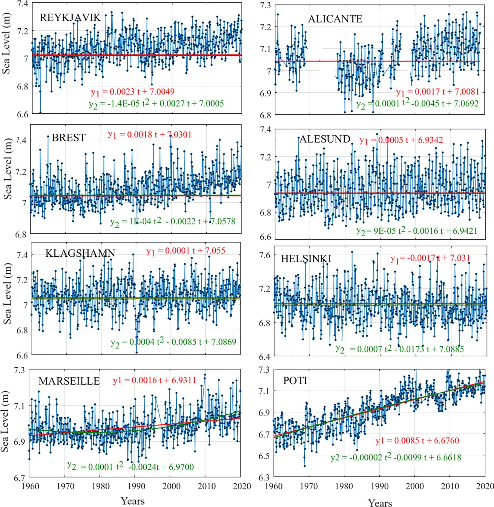
Figure 2 The 60-year-long tide gauge observation modeling using linear and quadratic approaches at eight sites along the European coastal area.

Table 2

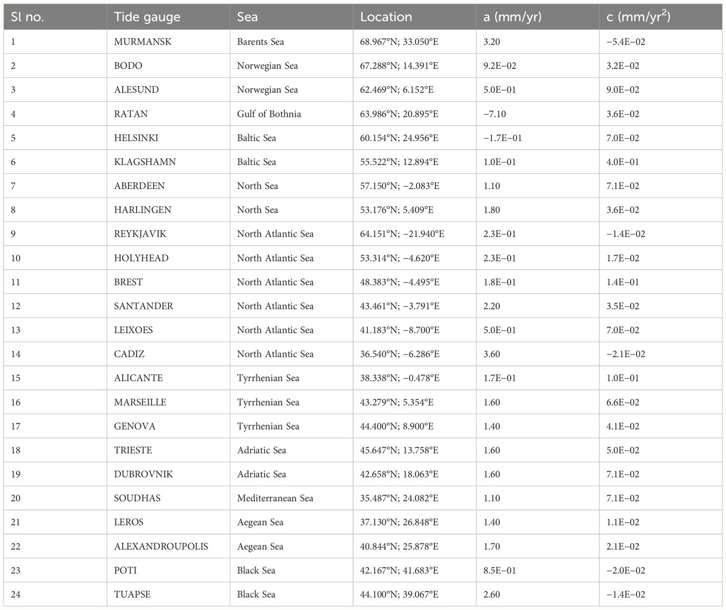
Table 2 The real-time sea-level observations from 24 tide gauge stations and their rare change.

The results show positive trends for almost every station (except RATAN and HELSINKI), but they have differences in rates of sea level rise (0.09 to 3.6 mm/yr) and acceleration (−5.4E−02 to 4.0E−01 mm/yr²). A rising trend in sea level with a minor rate of changes was observed at almost all tide gauge stations. The station MURMANSK, located in the coastal area of Barents Sea at the North of BODO, was connected with the Arctic Sea. We noticed that the sea-level trend increased to 3.2 mm/yr and had an acceleration of ~−0.054 mm/yr². Fu et al. (2021) analyzed variation in absolute sea level based on data from tide gauge measurements and multi-mission satellite altimetry in the Arctic during 1993–2018. They found that the trend of absolute sea levels ranged from −2.00 to 6.88 mm/yr except in the central region of the Arctic Ocean. The negative trend was mainly located in the high-latitude areas, while shallow water depth (<1 km) showed a positive trend. It has been noticed that the satellite-derived average secular absolute trend has been approximately 2.53 ± 0.42 mm/yr in the Arctic region (Fu et al., 2021). In this period (1993–2018), the tide gauge minimum value was in 1995 (~−10 SLA/cm) and the maximum in 2003 and 2017 (~10 SLA/cm). Here, SLA stands for sea level anomalies (SLA), which describes the difference between the actual sea surface height (SSH) and the mean sea surface height (MSSH). To analyze the vertical land motion (VLM) effect on sea-level change in the Arctic Sea, Fu et al. (2021) used a total of 11 global navigation satellite system (GNSS) stations for vertical displacement of which six were located near the tide gauge stations. The results showed that VLM ranges at ±10 cm at most of the stations. Ignoring the influences of atmospheric pressure, wind influence, and other factors of metrology, the absolute variability of sea level can be separated into the component of VLM and its changes relative to the crust along the Arctic Sea coast (Fu et al., 2021).

Stations BODO and ALESUND from the coastal area of the Norwegian Sea (Norway) show a 0.09 and 0.5 mm/yr increasing rate from 1960 to 2020, respectively. Breili et al. (2017) used tide gauge data from 1960 to 2010 and sea-level rates in the Norwegian Sea. They found that the rates range from 0.9 to 3.0 mm/yr with ±0.6 mm/yr uncertainty. These authors’ weighted average rise of sea-level calculation along the Norwegian coast was 2.0 ± 0.6 mm/yr. This rising rate was like the 20th-century global mean sea-level rise stated by the Intergovernmental Panel on Climate Change (IPCC, 2023). As per IPCC, during 1901–2010, the rise of global mean sea level reached 0.19 m (0.17 to 0.21 m). The VLM because of glacial isostatic adjustment (GIA) is a significant component of Norwegian relative sea-level change. GIA occurred because of crustal deformation, past loss of ice mass, and associated changes in the Earth’s gravity field. It has been seen that the VLM acceleration because of GIA in Norway is proportional to the present GIA rate factor of −0.0002 yr⁻¹ (Hünicke and Zorita, 2016). This rate is very low; hence, it can be assumed that the GIA effect on sea level along the Norwegian coast is constant and does not play any significant role on a continental time scale.

We included two stations, ABERDEEN and HARLINGEN, from the coastal area of the North Sea and found that the rising rates are 1.1 and 1.8 mm/yr, respectively, at those locations. As per our study, there is very low acceleration (0.071 mm/yr² at ABERDEEN and 0.036 mm/yr² at HARLINGEN), which is negligible. Wahl et al. (2013) studied the 1850–2011 data from the North Sea region and presented three time-series indices by taking the mean GIA-corrected tide gauge measurements for each year. Including GIA, their study of the relative change in sea level was based on VLM, which arises from tectonic movements, subsidence caused by ground fluid withdrawal, and geologic processes on regional and local scales. The time series were studied by Wahl et al. (2013). These researchers used singular spectrum analysis techniques and estimated regional sea-level acceleration in the last few decades. Although their estimated rate of linear trend was ~1.6 ± 0.9 mm/yr, there was no evidence of significant acceleration in the North Sea region. Stations (REYKJAVIK, HOLYHEAD, BREST, SANTANDER, LEIXOES, and CADIZ) located in the coastal area of the North Atlantic Sea were studied (Table 2). Although all these stations located at different parts of the North Atlantic Sea showed positive trends of sea-level rise, the rates of trends are low. Boers (2021) studied the circulation of Atlantic meridional overturning and found it in a stable condition in the last century. Their claim was based on salinity and surface temperature data across the Atlantic Ocean basin.

The SOUDHAS station located in the coastal area of the Mediterranean Sea shows a rise of trend of ~1.1 mm/yr with 0.007 mm/yr² of acceleration, showing near-stability in the water surface. The nearest other two stations, LEROS and ALEXANDROUPOLIS, at the coastal area of the Aegean Sea show a rise of trend of ~1.4 and 1.7 mm/yr, respectively. Several studies conducted in the Aegean Sea and the Mediterranean Sea in different timescales showed positive trends of sea-level measurement except for Vigo et al. (2005), who estimated a negative trend of ~−0.6 mm/yr for the 1993–2003 dataset. Cazenave et al. (2002) used tide gauge data in the Aegean Sea and estimated a sea-level trend of ~0.62 mm/yr during 1993–1998. A quick rise in sea level was observed during the 1990s induced by both mass components and steric sea level. In succeeding decades, it lost its increasing rates due to the steric sea level. Galassi and Spada (2014) forecasted the sea-level measurements for 2040–2050 relative to the 1990–2000 measurements. Their result for the Aegean Sea suggests an increase in water level between 14 and 27.5 cm. Tsimplis et al. (2011) combined steric sea-level records in the Mediterranean Sea during 1945–2002 and an atmospheric forcing model during the period of 1958–2001. Their results showed a negative trend across the Mediterranean Sea, especially in the eastern Mediterranean Basin; it varied from −0.9 to 0 mm/yr. Bonaduce et al. (2016) noticed a positive trend of 2.44 ± 0.5 mm/yr in the Mediterranean basin using data from tide gauge and satellite altimetry observations from 1993 through 2012. Taibi and Haddad (2019) used the 1993–2015 data and estimated a significant trend of 1.48 to 8.72 mm/yr. Although the collision between Arabian, Eurasian, and African plates generates very complex microplate regimes in the Mediterranean Sea especially relative to VLM, Peltier (2000) estimated motion of VLM ± 0.1/0.2 mm/yr in the Mediterranean Sea region including the Black Sea area. Therefore, the influence of GIA can be ignored in terms of tectonic movements (Garcia et al., 2007). The Aegean Sea may have a slightly different tendency than the global tendency because of the input of freshwater (Talley et al., 2011). This made the Aegean sea level different from others like the Mediterranean and the Black Sea because of salinification, with the faster rate of heating affecting the steric sea level (Talley et al., 2011). The area of the Aegean Sea is rapidly deforming and seismically active. In the region including Greece and western Turkey, several destructive earthquakes have occurred in the last several years to be stated in order to make a meaningful sentence. The subduction of the African block northward occurred in this region, which uplifted Crete Island (the north side of the Hellenic Arc) (Rahl et al., 2004).

Stations TRIESTE and DUBROVNIK are located in the coastal area of the Adriatic Sea and show a sea level rising trend of ~1.6 mm/yr. The Adriatic Sea assists as a sample where derived observation ensemble modeling of sea level is imperative for consistent forecasts of induced cyclone-driven wind floods in Venice and other coastal cities along the northern coast of the Adriatic Sea. The long-term multidecadal fluctuations of sea-level excesses in the Mediterranean Sea have been seen in long-term tide gauge observations, such as since the 1930s Trieste site and other northern sites of the Adriatic. Raicich (2003) recognized the extreme frequency declines in Trieste tide gauge measurements from 1940 to 2000, without a clear trend of tidal intensity. In contrast, Masina and Lamberti (2013) recognized a small increment in the sea-level magnitude excesses in the northern Adriatic Sea, which was connected with a strengthening of the bora wind during the 1990s. Lionello et al. (2021) stated that the flooding frequency resulting from storm surges has enlarged in Venice, since the mid-20th century, although they related this to the relative sea level rise effect rather than to the continued storminess trend. At inter-annual time scales, extreme sea-level changes are correlated with the oscillation in the North Atlantic Ocean (Masina and Lamberti, 2013), even after the elimination of the annual mean sea-level signal. According to Cid et al. (2016), the Gulf of Gabes in Tunisia and the Adriatic and Aegean coasts underwent a very high number of extreme events in sea level every year from 1948 to 2013. The western coast of the Black Sea is most exposed to storm surges (Bresson et al., 2018). Deltas, low elevation, and sinking land regions too have high flood risks during these extreme events (Hereher, 2015; Grases et al., 2020; Ferrarin et al., 2021).

3.2 Least-squares harmonic estimation tidal modeling

We made a 60-year (1961 to 2020) time-series plot of three tide gauge stations, BODO, BREST, and SOUDHAS (Figure 3), which are located in the Norwegian, North Atlantic, and Mediterranean Sea, respectively. The black dots in Figure 3 show sea level height, and the blue lines are the HA-estimated tidal models. Here, the Fourier coefficients, A_i and B_i, were chosen up to 8 to model the tide gauge. It is clear from the modeled data that the sea level of the Norwegian Sea (BODO) constantly varied between 6.8 and 7. 2 m in the 60 years. The BREST station in the North Atlantic Sea shows variation from 7.0 to 7.2 m with some increment. The SOUDHAS in the Mediterranean varies from 6.98 to 7.14 m with some increment. The results show that the level of water gains its top value during the months of summer months from June to September. In general, the meteorological force impact is attributed especially to pressure in the atmosphere, which decreases to its lowest levels during the summer months (Sultan et al., 2000; Afshar-Kaveh et al., 2020). In contrast, when the atmospheric pressure reaches its highest levels at the time of winter, the height of water generally becomes the lowest due to the inverse relationship between the sea surface and meteorological elements. The variations in the water level are mainly connected with the astronomical tidal phenomenon. The frequency of the main diurnal tidal parameters (cycles per day) is estimated from the tide gauge stations (Table 3). The smaller and higher tidal frequencies of these stations indicate their stability in terms of the sea-surface variation. For example, if any station is in an inland sea, it shows smaller tide parameters. Here in these three stations, no significant difference in tidal parameters has been seen, which indicates that their stability in terms of tidal variation is almost the same. The records of sea level displayed a maximum annual tidal variation of ~4.32 m, from 1.66 to −2.66 m. Generally, the maximum range of tides is noted during the spring tide, and during the neap tide, the range of tides hardly exceeds approximately 2.5 m. To underrate the accuracy of HA, we estimated the residual values from observed and modeled data. The residual plot with the thresholds of the observed HA-modeled data at these stations is shown in Figure 4, which varies from −0.2 to 0.2 m. The histogram plot of residuals ranges from −0.2 to 0.2 m, and their approximation is almost a normal distribution. Here, the mean of error is close to or almost equivalent to zero; therefore, the modeled results can be recognized as an unbiased estimation as per the rule of standard normal distribution. Finally, we can conclude that the error distribution predicted by HA modeling is more reasonable. Further study of the Taylor correlation coefficients between observed and HA-modeled tide gauges along with satellite altimetry is discussed in Section 3.3.

Figure 3

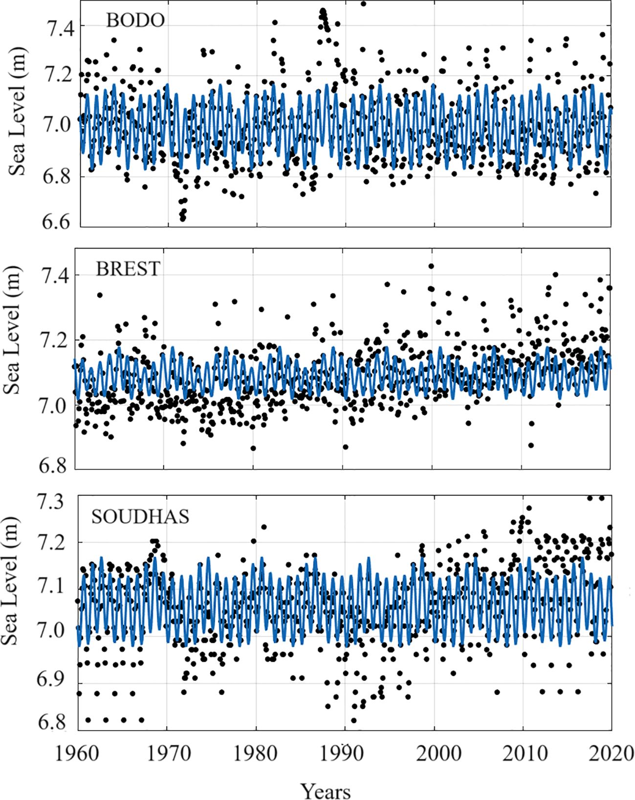
Figure 3 Least-squares harmonic estimation tidal modeling of 60-year tide gauge measurements time series in European coast.

Table 3

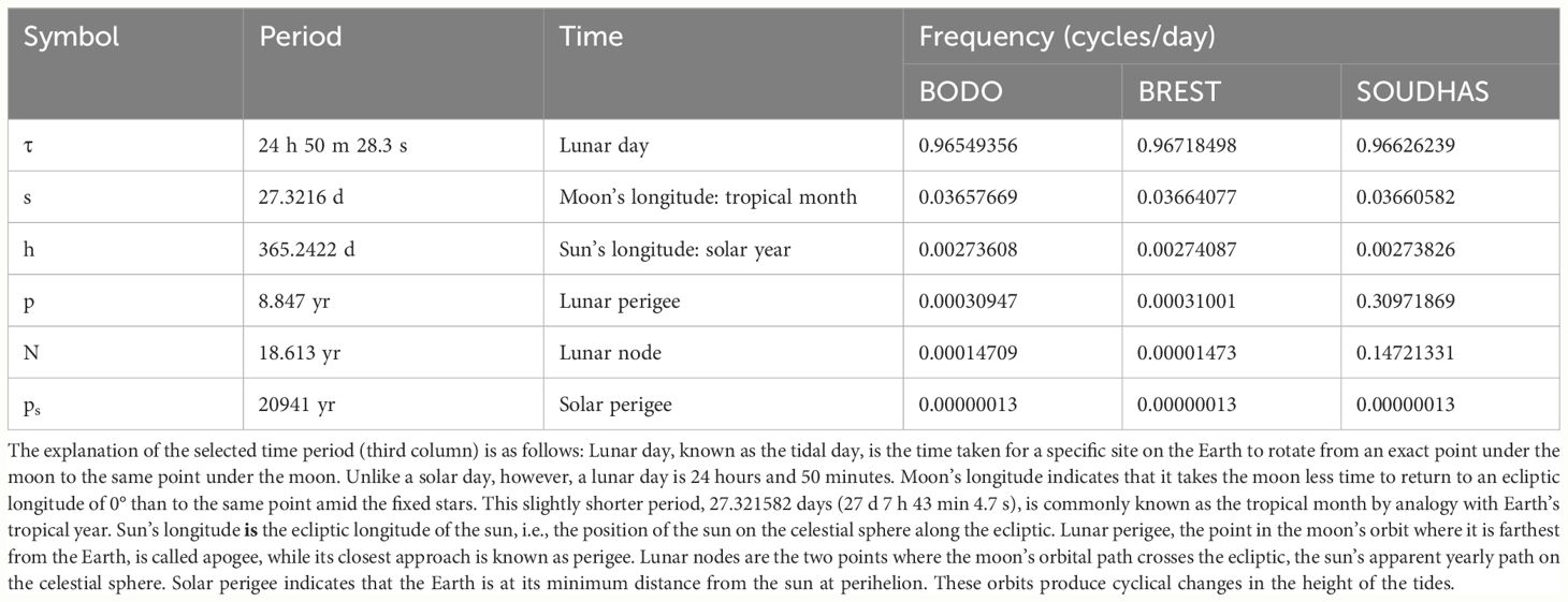
Table 3 Fundamental estimated tidal frequencies in certain time periods.

Figure 4

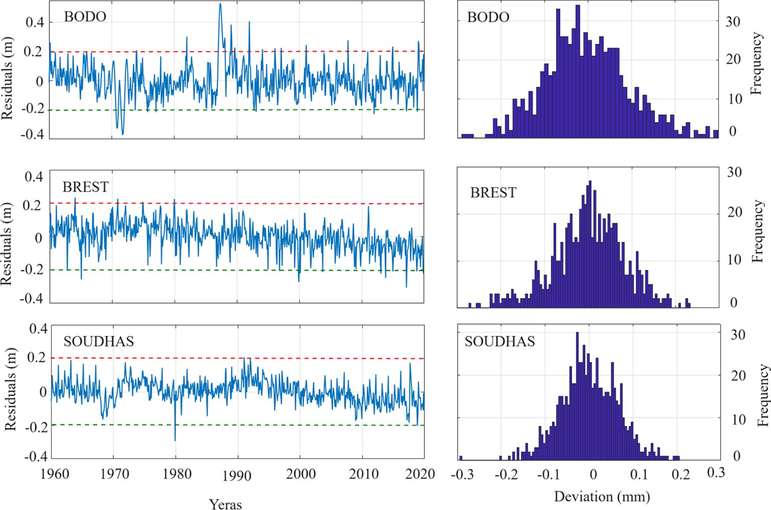
Figure 4 Residuals plot with threshold value (−0.4 to 0.4) and the histogram of residuals for tide gauge station (selected in Figure 3).

3.3 Satellite altimetry and sea-level topography

The sea-level measurements of tide gauges are recorded relative to benchmarks in the ground such as datum. Hence, it is possible that the inclusion of some kind of vertical ground motion can affect the local level. The sea-level measurements taken by satellite altimetry were measured concerning geocentric reference and not affected by vertical land motion. To validate the altimetry observations with tide gauge records, a comparative analysis was performed. The sea-level trend was estimated for each tide gauge by comparison of the closest grid point of satellite altimetry using Equation 7 and 8 for six stations (Figure 5). The derived PSMSL tide gauge data are plotted with blue lines, while the satellite altimetry is shown with orange lines. In Figure 5, the observation time period during the years (1993–2020) is displayed by the horizontal axis, and the tide gauge measurement (satellite altimetry and PSMSL) deviation from the mean values is shown by the vertical axis. Although the physical trend looks the same in both time series, they have low agreements in a few cases and exhibit distinct variations. To understand more detail between PSMSL tide gauge and satellite altimetry, we used the Taylor correlation plots (Figure 6). Moreover, we used HA and predicted new modeled time series of PSMSL tide gauge measurements. In Figure 6, SA indicates the correlation coefficient between observed satellite altimetry and PSMSL tide gauge, while FT indicates the correlation coefficient between HA predicted PSMSL tide gauge and measured PSMSL tide gauge. The results of correlation coefficients between the PSMSL tide gauge and others (satellite altimetry and HA tide gauge) at each station vary; some of them have low correlation, while others have high correlation. For example, at MURMANSK, the satellite altimetry and PSMSL tide gauge have the lowest correlation coefficient (0.42), while at HARLINGEN, the satellite altimetry and PSMSL tide gauge have the highest magnitude (0.80). Note that the tide gauge measurements reflect a relative change in sea level and that absolute sea level changes are captured by satellite altimetry. Many factors can affect the big differences in the trend of sea level between the tide gauge and the satellite-derived result. For example, the satellite data with low precision in the coastal zones and the effective data influence coverages of satellite altimetry (Fu et al., 2021). We compared the trend of sea level between the station of the tide gauge and the closest grid satellite-derived product. Theoretically, the error is possible between them if they have a large distance. Therefore, the distance influence should not be ignored. The correlation coefficient between the HA-predicted and observed tide gauges also varies for each station. For example, at TRIESTE, the correlation coefficient is the lowest (0.53), while at HELENSKI, it is the highest (0.93). The Fourier coefficients A_i and B_i predict that the tide gauge time series above the coefficients are neglected. In the HA, the time series with a high standard deviation (STD) shows the highest correlation coefficient, and that with the lowest STD displays the smallest coefficient (STD indicated as black points in Figure 6).

Figure 5

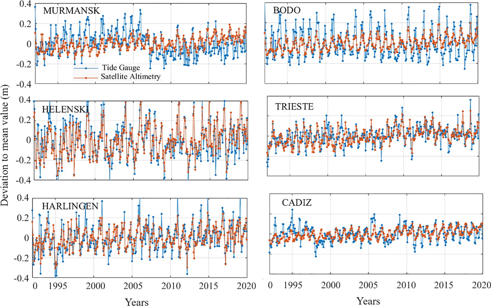
Figure 5 The comparative analysis between the newly estimated time series of both satellite altimetry (1993–2020) and Permanent Service for Mean Sea Level (PSMSL) tide gauge datasets at six sites.

Figure 6

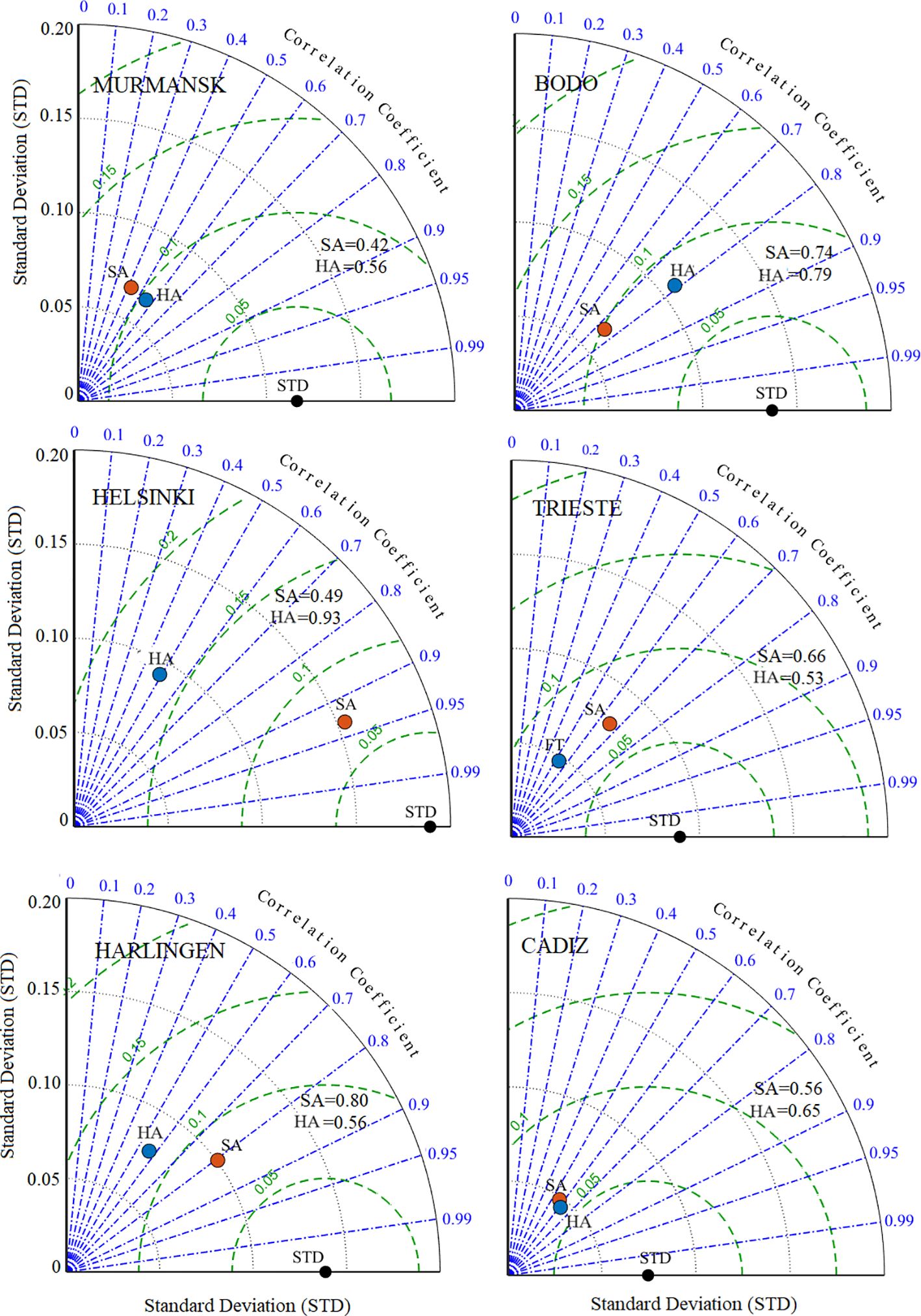
Figure 6 Taylor correlation coefficient plot among Permanent Service for Mean Sea Level (PSMSL), satellite altimetry (SA), and harmonic analysis (HA) molded time series (1993–2020).

Bathymetric data were downloaded from Internet ref-1 at an extension of 28°N–78°N and 30°W–55°E to determine the deposition pattern in marine depressions and ridges as well as the slope direction of undulating terrain. These 3D data were processed in the ArcGIS 10.8.1 (ESRI, 2020) platform. The offshore topographic slope direction and slope range with contour spacing from the sea to the associated coastline are shown in Figure 7. The figure shows the slope direction map about the aspect slope map in NE and E directions. The ridges were predicted to have multi-slope directions. In the offshore regions, multidirectional ridges were noticed. The depressed land may be indicated by the flat topography. The area with a steep slope toward the sea was defined by the close-spaced contours. The ridges with multidirectional slopes were identified by patches of contours on the seafloor (Figure 8). The slope changes to moderate/steep toward the east, west, and southeast as per the Digital Elevation Model (DEM)-based contour map. There can be an abrupt change in slope from the coastline toward the sea.

Figure 7

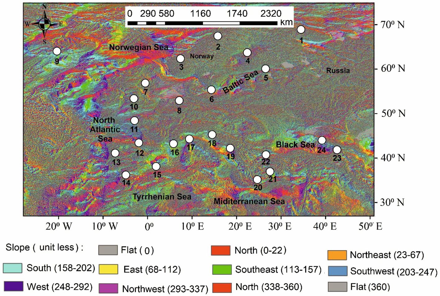
Figure 7 Map of slope direction derived from undersea DEM data. Multi-slope directions of slope analysis are available for both onshore and offshore topography.

Figure 8

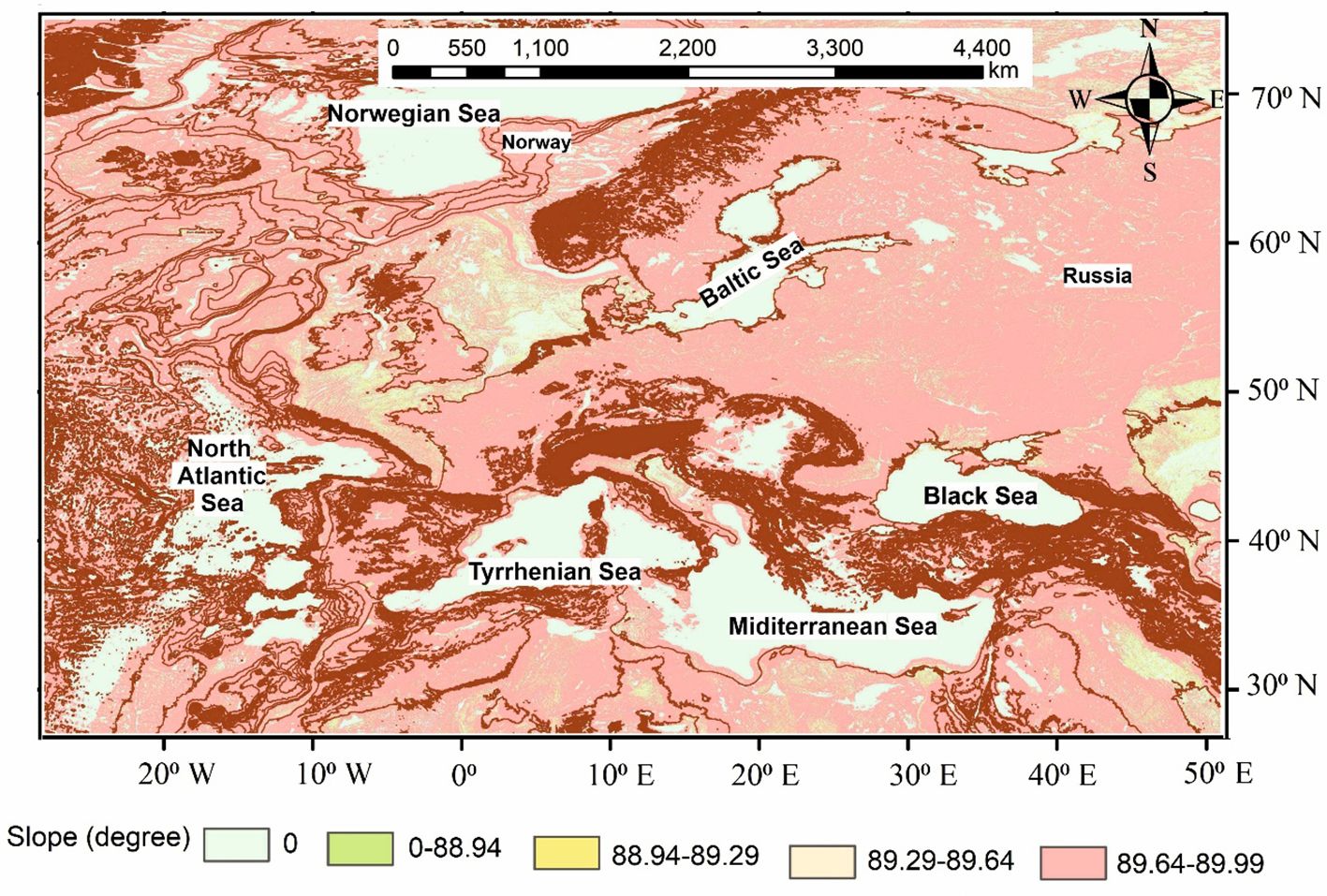
Figure 8 Detailed contour mapping with slope amount (0°–90°) and degree at 100-m intervals on land and underwater.

4 Conclusions

The study investigated tide gauge observation along the European coast during the 60-year period (1961–2020). A total of 24 stations were included in the current study, which are located at the coastal areas of different seas such as the Barents Sea, Gulf of Bothnia, Norwegian Sea, North Sea, North Atlantic Sea, Baltic Sea, Tyrrhenian Sea Mediterranean Sea, Aegean Sea, and Black Sea along ~68,000 km of the European coast. The study points out an almost positive rate of trend of sea-level rise at almost all stations. The results showed that the sea-level trend increased to 3.2 mm/yr and accelerated ~−0.054 mm/yr² along the Arctic Sea coast. Along the Norwegian Sea, increasing rates of 0.09 and 0.5 mm/yr were observed during our selected period (1960 to 2020). It was seen that the GIA effect on sea level along the Norwegian coast is constant and does not play a significant role on a continental time scale. The rising rates were from the coastal area of the North Sea and were found to vary from 1.1 to 1.8 mm/yr with low to very low acceleration (0.036–0.071 mm/yr²). The station located in the coastal area of the Mediterranean Sea shows a rise of trend of ~1.1 mm/yr with 0.007 mm/yr² of acceleration, showing near stability in the water surface. The coastal area of the Aegean Sea shows a rise of trend of ~1.4–1.7 mm/yr. The Aegean Sea may have a slightly different tendency than the global tendency because of the input of freshwater. The area of the Aegean Sea is a rapidly deforming and seismically active region. Stations located in the Adriatic Sea’s coastal area show a rising sea-level trend of ~1.6 mm/yr. The Adriatic Sea assists as a sample where derived observation ensemble modeling of sea level is imperative for consistent forecasts of induced cyclone-driven wind floods in Venice and coastal cities along the northern coast of the Adriatic Sea.

The regional tidal model is estimated by utilizing the tide gauge stations, and a comparative analysis was carried out. The histogram plot of residuals between observed and HA-modeled values ranges from −0.2 to 0.2 m, and their approximation shows almost a normal distribution. This can be inferred that the error distribution predicted by HA modeling is more reasonable. This kind of modeling provides primary information and possibility for the coastal area of Europe. Also, the determination of tidal parameters on the coast of selected seas is significant from many viewpoints such as big coastal buildings (energy facilities, port, etc.), tourist facilities, biodiversity, and fishing. Particularly, during the time of new building construction, tidal parameters must be considered by engineers to avoid tidal damage. The satellite altimetry data (1993–2020) from the nearest grid points have been used, and studying their relationship with tide gauge observations has been attempted. The correlation coefficients among the tide gauge, tidal modeling, and satellite altimetry are not high. This shows that the global near-shore regions’ sea level information is imperfect or, at least, the resolution and accuracy at temporal and spatial levels need to be upgraded.

Data availability statement

Publicly available datasets were analyzed in this study. This data can be found here: https://psmsl.org/data/.

Author contributions

KA: Writing – original draft, Writing – review & editing. JW: Writing – review & editing. KW: Writing – review & editing. MB: Writing – review & editing. SM: Writing – review & editing.

Funding

The author(s) declare financial support was received for the research, authorship, and/or publication of this article. The research was funded by the Warsaw University of Technology within the Excellence Initiative: Research University (IDUB) program.

Acknowledgments

We thank PSMSL and Satellite Altimetry agencies for providing public access to data used in the current study.

Conflict of interest

The authors declare that the research was conducted in the absence of any commercial or financial relationships that could be construed as a potential conflict of interest.

Publisher’s note

All claims expressed in this article are solely those of the authors and do not necessarily represent those of their affiliated organizations, or those of the publisher, the editors and the reviewers. Any product that may be evaluated in this article, or claim that may be made by its manufacturer, is not guaranteed or endorsed by the publisher.

Abbreviations

C3S, Copernicus Climate Change Service; DMB, digital bathymetric model; DEM, Digital Elevation Model; GEBCO, General Bathymetric Chart of the Oceans; GIA, glacial isostatic adjustment; GIS, Geographical Information System; GNSS, global navigation satellite system; HA, harmonic analysis; IHRS, International Height Reference System; IPCC, Intergovernmental Panel on Climate Change; MSSH, mean sea surface height; PSMSL, Permanent Service for Mean Sea Level; SA, satellite altimetry; SLA, sea level anomalies; SSH, sea surface height; TG, tide gauge; VLM, vertical land motion

References

Afshar-Kaveh N., Nazarali M., Pattiaratchi C. (2020). Relationship between the Persian Gulf sea-level fluctuations and meteorological forcing. J. Mar. Sci. Eng. 8, 285. doi: 10.3390/jmse8040285

CrossRef Full Text | Google Scholar

Amante C., Eakins B. W. (2008). E TOPO1 1Arc-MinuteGlobalReliefModel: Procedures, Data Sources and Analysis (Boulder, Colorado: National Geophysical Data Center, NESDIS, NOAA and U.S. Department of Commerce). Available online at: http://www.ngdc.noaa.gov/mgg/global/global.html (Accessed Apr.30, 2011).

Google Scholar

Ansari K., Bae T. S., Inyurt S. (2020). Global positioning system interferometric reflectometry for accurate tide gauge measurement: Insights from South Beach, Oregon, United States, Acta Astronautica 173, 356–362. doi: 10.1016/j.actaastro.2020.04.060

CrossRef Full Text | Google Scholar

Ansari K. (2022). Modelling and spectral analysis of sea-level trend over Indian coastal area. Mar. Geophys. Res. 43, 1–9. doi: 10.1007/s11001-022-09468-y

CrossRef Full Text | Google Scholar

Ansari K., Bae T. S. (2021). Modelling and mitigation of real-time sea level measurement over the coastal area of Japan. Mar. Geophys. Res. 42, 1–15. doi: 10.1007/s11001-021-09460-y

CrossRef Full Text | Google Scholar

Ansari K., Seok H. W., Jamjareegulgarn P. (2022a). Quasi zenith satellite system-reflectometry for sea-level measurement and implication of machine learning methodology. Sci. Rep. 12, 21445. doi: 10.1038/s41598-022-25994-6

PubMed Abstract | CrossRef Full Text | Google Scholar

Ansari K., de Oliveira-Junior J. F., RidoutJamjareegulgarn P. (2022b). Spatial changes of ocean circulation along the coast of Gulf of Thailand using tide gauge measurements. IEEE Access 10, 130795–130805. doi: 10.1109/ACCESS.2022.3229212

CrossRef Full Text | Google Scholar

Araújo M. A. (2022). Sea level changes: the data available at the PSMSL and SONEL and the results of satellite altimetry. 1–19. doi: 10.21203/rs.3.rs-2383126/v1

CrossRef Full Text | Google Scholar

Armitage T. W., Bacon S., Ridout A. L., Thomas S. F., Aksenov Y., Wingham D. J. (2016). Arctic sea surface height variability and change from satellite radar altimetry and GRACE 2003–2014. J. Geophys. Res.: Oceans 121, 4303–4322. doi: 10.1002/2015JC011579

CrossRef Full Text | Google Scholar

Available online at: https://download.gebco.net/ (Accessed 12-Dec-2023). Internet ref-1.

Google Scholar

Available online at: https://www.gebco.net/data_and_products/gridded_bathymetry_data/#global (Accessed 12-Dec-2023). Internet ref-2.

Google Scholar

Balogun A. L., Adebisi N. (2021). Sea level prediction using ARIMA, SVR and LSTM neural network: assessing the impact of ensemble Ocean-Atmospheric processes on models’ accuracy. Geom. Natural Hazards Risk 12, 653–674. doi: 10.1080/19475705.2021.1887372

CrossRef Full Text | Google Scholar

Beckley B. D., Lemoine F. G., Luthcke S. B., Ray R. D., Zelensky N. P. (2007). A reassessment of global and regional mean sea level trends from TOPEX and Jason-1 altimetry based on revised reference frame and orbits. Geophys. Res. Lett. 34, 1–5. doi: 10.1029/2007GL030002

CrossRef Full Text | Google Scholar

Beenstock M., Felsenstein D., Frank E., Reingewertz Y. (2015). Tide gauge location and the measurement of global sea level rise. Environ. Ecol. Stat 22, 179–206. doi: 10.1007/s10651-014-0293-4

CrossRef Full Text | Google Scholar

Boers N. (2021). Observation-based early-warning signals for a collapse of the Atlantic Meridional Overturning Circulation. Nat. Climate Change 11, 680–688. doi: 10.1038/s41558-021-01097-4

CrossRef Full Text | Google Scholar

Bonaduce A., Pinardi N., Oddo P., Spada G., Larnicol G. (2016). Sea-level variability in the Mediterranean Sea from altimetry and tide gauges. Climate Dynam. 47, 2851–2866. doi: 10.1007/s00382-016-3001-2

CrossRef Full Text | Google Scholar

Boretti A. (2021). Nonlinear absolute sea-level patterns in the long-term-trend tide gauges of the East Coast of North America. Nonlinear Eng. 10, 1–15. doi: 10.1515/nleng-2021-0001

CrossRef Full Text | Google Scholar

Born G. H., Dunne J. A., Lame D. B. (1979). Seasat mission overview. Science 204, 1405–1406. doi: 10.1126/science.204.4400.1405

PubMed Abstract | CrossRef Full Text | Google Scholar

Breili K., Simpson M. J., Nilsen J.E.Ø. (2017). Observed sea-level changes along the Norwegian Coast. J. Mar. Sci. Eng. 5, 29. doi: 10.3390/jmse5030029

CrossRef Full Text | Google Scholar

Bresson É., Arbogast P., Aouf L., Paradis D., Kortcheva A., Bogatchev A., et al. (2018). On the improvement of wave and storm surge hindcasts by downscaled atmospheric forcing: application to historical storms. Natural Hazards Earth Sys. Sci. 18, 997–1012. doi: 10.5194/nhess-18-997-2018

CrossRef Full Text | Google Scholar

Buchanan M. K., Oppenheimer M., Kopp R. E. (2017). Amplification of flood frequencies with local sea level rise and emerging flood regimes. Environ. Res. Lett. 12, 064009. doi: 10.1088/1748-9326/aa6cb3

CrossRef Full Text | Google Scholar

C3S (2023). Global Ocean Gridded L4 Sea Surface Heights and Derived Variables Reprocessed Copernicus Climate Change Service (Accessed 12 Nov 2023).

Google Scholar

Cazenave A., Bonnefond P., Mercier F., Dominh K., Toumazou V. (2002). Sea level variations in the Mediterranean Sea and Black Sea from satellite altimetry and tide gauges. Global Planet. Change 34, 59–86. doi: 10.1016/S0921-8181(02)00106-6

CrossRef Full Text | Google Scholar

Cazenave A., Nerem R. S. (2004). Present-day sea level change: Observations and causes. Rev. Geophys. 42, 1–20. doi: 10.1029/2003RG000139

CrossRef Full Text | Google Scholar

Cid A., Menéndez M., Castanedo S., Abascal A. J., Méndez F. J., Medina R. (2016). Long-term changes in the frequency, intensity and duration of extreme storm surge events in southern Europe. Climate Dynam. 46, 1503–1516. doi: 10.1007/s00382-015-2659-1

CrossRef Full Text | Google Scholar

Cipollini P., Calafat F. M., Jevrejeva S., Melet A., Prandi P. (2017). Monitoring sea level in the coastal zone with satellite altimetry and tide gauges. Integr. study mean sea level its components. 58, 35–59. doi: 10.1007/978-3-319-56490-6_3

CrossRef Full Text | Google Scholar

Emery K. O., Aubrey D. G. (2012). Sea levels, land levels, and tide gauges (Woods Hole, MA, USA: Springer Science & Business Media).

Google Scholar

Erkoç M. H., Doğan U. (2022). Regional tidal modelling using tide gauges and satellite altimetry data in south-west coast of Turkey. KSCE J. Civil Eng. 26, 4052–4061. doi: 10.1007/s12205-022-0320-1

CrossRef Full Text | Google Scholar

ESRI (2020). ArcGIS Desktop: Release 10 (Redlands, CA: Environmental Systems Research Institute).

Google Scholar

Ezer T. (2023). Sea level acceleration and variability in the Chesapeake Bay: past trends, future projections, and spatial variations within the Bay. Ocean Dynam. 73, 23–34. doi: 10.1007/s10236-022-01536-6

CrossRef Full Text | Google Scholar

Ferrarin C., Bajo M., Benetazzo A., Cavaleri L., Chiggiato J., Davison S., et al. (2021). Local and large-scale controls of the exceptional Venice floods of November 2019. Prog. Oceanogr. 197, 102628. doi: 10.1016/j.pocean.2021.102628

CrossRef Full Text | Google Scholar

Fu Y., Feng Y., Zhou D., Zhou X. (2021). Absolute sea level variability of Arctic Ocean in 1993–2018 from satellite altimetry and tide gauge observations. Acta Oceanol. Sinica. 40, 76–83. doi: 10.1007/s13131-021-1820-4

CrossRef Full Text | Google Scholar

Galassi G., Spada G. (2014). Sea-level rise in the Mediterranean Sea by 2050: Roles of terrestrial ice melt, steric effects and glacial isostatic adjustment. Global Planet. Change 123, 55–66. doi: 10.1016/j.gloplacha.2014.10.007

CrossRef Full Text | Google Scholar

Garcia D., Vigo I., Chao B. F., Martinez M. C. (2007). Vertical crustal motion along the Mediterranean and Black Sea coast derived from ocean altimetry and tide gauge data. Pure Appl. Geophys. 164, 851–863. doi: 10.1007/s00024-007-0193-8

CrossRef Full Text | Google Scholar

Ghazali N. H. M., Awang N. A., Mahmud M., Mokhtar A. (2018). Impact of sea level rise and tsunami on coastal areas of north-West Peninsular Malaysia. Irrig. Drain. 67, 119–129. doi: 10.1002/ird.2244

CrossRef Full Text | Google Scholar

Grases A., Gracia V., García-León M., Lin-Ye J., Sierra J. P. (2020). Coastal flooding and erosion under a changing climate: implications at a low-lying coast (Ebro Delta). Water 12, 1–26. doi: 10.3390/w12020346

CrossRef Full Text | Google Scholar

Haq B. U., Schutter S. R. (2008). A chronology of Paleozoic sea-level changes. Science 322, 64–68. doi: 10.1126/science.1161648

PubMed Abstract | CrossRef Full Text | Google Scholar

He X., Montillet J. P., Fernandes R., Melbourne T. I., Jiang W., Huang Z. (2022). Sea level rise estimation on the pacific coast from Southern California to Vancouver Island. Remote Sens. 14, 4339. doi: 10.3390/rs14174339

CrossRef Full Text | Google Scholar

Hell B. (2011). Mapping bathymetry: From measurement to applications. Stockholm, Sweden: Department of Geological Sciences, Stockholm University.

Google Scholar

Hereher M. E. (2015). Coastal vulnerability assessment for Egypt’s Mediterranean coast. Geom. Natural Hazards Risk 6, 342–355. doi: 10.1080/19475705.2013.845115

CrossRef Full Text | Google Scholar

Holgate S. J., Matthews A., Woodworth P. L., Rickards L. J., Tamisiea M. E., Bradshaw E., et al. (2013). New data systems and products at the permanent service for mean sea level. J. Coast. Res. 29, 493–504. doi: 10.2112/JCOASTRES-D-12-00175.1

CrossRef Full Text | Google Scholar

Horn W. (1960). Some recent approaches to tidal problems. Int. Hydrogr. Rev. 65–88.

Google Scholar

Hünicke B., Zorita E. (2016). Statistical analysis of the acceleration of Baltic mean sea-level rise 1900–2012. Front. Mar. Sci. 3. doi: 10.3389/fmars.2016.00125

CrossRef Full Text | Google Scholar

IPCC, Core Writing Team (2023). “Climate Change 2023: Synthesis Report, Summary for Policymakers,” in Contribution of Working Groups I, II and III to the Sixth Assessment Report of the Intergovernmental Panel on Climate Change. Eds. Lee H., Romero J. (IPCC, Geneva, Switzerland).

Google Scholar

Iz H. B., Shum C. K. (2022). Minimum record length for detecting a prospective uniform sea level acceleration at a tide gauge station. All Earth 34, 8–15. doi: 10.1080/27669645.2022.2045697

CrossRef Full Text | Google Scholar

Klenke M., Schenke H. W. (2002). A new bathymetric model for the central Fram Strait. Mar. Geophys. Res. 23, 367–378. doi: 10.1023/A:1025764206736

CrossRef Full Text | Google Scholar

Lambeck K. (2014). “Of moon and land, ice and strand: sea level during glacial cycles,” in Of moon and land, ice and strand, 1–86. Rome, Italy: Accademia Nazionale dei Lincei. Available at: https://www.torrossa.com/en/resources/an/3048121.

Google Scholar

Lionello P., Barriopedro D., Ferrarin C., Nicholls R. J., Orlić M., Raicich F., et al. (2021). Extreme floods of Venice: characteristics, dynamics, past and future evolution. Natural Hazards Earth Sys. Sci. 21, 2705–2731. doi: 10.5194/nhess-21-2705-2021

CrossRef Full Text | Google Scholar

Müller R. D., Sdrolias M., Gaina C., Steinberger B., Heine C. (2008). Long-term sea-level fluctuations driven by ocean basin dynamics. Science 319, 1357–1362. doi: 10.1126/science.115154

PubMed Abstract | CrossRef Full Text | Google Scholar

Masina M., Lamberti A. (2013). A nonstationary analysis for the Northern Adriatic extreme sea levels. J. Geophys. Res.: Oceans 118, 3999–4016. doi: 10.1002/jgrc.20313

CrossRef Full Text | Google Scholar

Mey J., Scherler D., Wickert A. D., Egholm D. L., Tesauro M., Schildgen T. F., et al. (2016). Glacial isostatic uplift of the European Alps. Nat. Commun. 7, 13382. doi: 10.1038/ncomms13382

PubMed Abstract | CrossRef Full Text | Google Scholar

Miller K. G., MouNtaiN G. S., WriGht J. D., Browning J. V. (2011). A 180-million-year record of sea level and ice volume variations from continental margin and deep-sea isotopic records. Oceanography 24, 40–53. doi: 10.5670/oceanog

CrossRef Full Text | Google Scholar

Parker A. (2016). Sea level rise and land subsidence contributions to the signals from the tide gauges of China. Nonlinear Eng. 5, 115–122. doi: 10.1515/nleng-2015-0033

CrossRef Full Text | Google Scholar

Parker A. (2018). Sea level oscillations in Japan and China since the start of the 20th century and consequences for coastal management-Part 2: China pearl river delta region. Ocean Coast. Manage. 163, 456–465. doi: 10.1016/j.ocecoaman.2018.12.031

CrossRef Full Text | Google Scholar

Parker A., Saleem M. S., Lawson M. (2013). Sea-level trend analysis for coastal management. Ocean Coast. Manage. 73, 63–81. doi: 10.1016/j.ocecoaman.2012.12.005

CrossRef Full Text | Google Scholar

Peltier W. R. (2000). “ICE4G (VM2) glacial isostatic adjustment corrections,” in Sea Level Rise: History and Consequences. Eds. Douglas B. C., Kearney M. S., Leatherman S. P. (Academic Press, San Diego).

Google Scholar

Prasanna H. M. I., Gunathilaka M. D. E. K., Iz H. B. (2023). Sea level variability at Colombo, Sri Lanka inferred from the conflation of satellite altimetry and tide gauge measurements 51 (2), 205–214. doi: 10.4038/jnsfsr.v51i2.10713

CrossRef Full Text | Google Scholar

Qu Y., Jevrejeva S., Wang S. (2023). Unraveling regional patterns of sea level acceleration over the China Seas. Remote Sens. 15, 4448. doi: 10.3390/rs15184448

CrossRef Full Text | Google Scholar

Rahl J., Fassoulas C., Brandon M. T. (2004). “Exhumation of high-pressure metamorphic rocks within an active convergent margin,” in Crete, Greece: A field guide. In Field Trip Guidebook for the 32nd International Geological Congress. Eds. Guerrieri L., Rischia I., Serva L. (Italian Agency for the Environmental Protection and Technical Services, Rome), 1–36.

Google Scholar

Raicich F. (2003). Recent evolution of sea-level extremes at Trieste (Northern Adriatic). Continent. Shelf Res. 23, 225–235. doi: 10.1016/S0278-4343(02)00224-8

CrossRef Full Text | Google Scholar

Shaw R., Mukherjee S. (2022). The development of carbon capture and storage (CCS) in India: A critical review. Carbon Capt. Sci. Technol. 2, 100036. doi: 10.1016/j.ccst.2022.100036

CrossRef Full Text | Google Scholar

Sultan S. A. R., Moamar M. O., El-Ghribi N. M., Williams R. (2000). Sea level changes along the Saudi coast of the Arabian Gulf. Available online at: http://nopr.niscair.res.in/handle/123456789/25532.

Google Scholar

Taherkhani M., Vitousek S., Barnard P. L., Frazer N., Anderson T. R., Fletcher C. H. (2020). Sea-level rise exponentially increases coastal flood frequency. Sci. Rep. 10, 6466. doi: 10.1038/s41598-020-62188-4

PubMed Abstract | CrossRef Full Text | Google Scholar

Taibi H., Haddad M. (2019). Estimating trends of the Mediterranean Sea level changes from tide gauge and satellite altimetry data, (1993–2015). J. Oceanol. Limnol. 37, 1176–1185. doi: 10.1007/s00343-019-8164-3

CrossRef Full Text | Google Scholar

Talley L., Pickard G., Emery W. J., Swift J. (2011). Descriptive Physical Oceanography: An Introduction. 6th ed (Boston, MA: Academic Press).

Google Scholar

Tsimplis M., Spada G., Marcos M., Flemming N. (2011). Multi-decadal sea level trends and land movements in the Mediterranean Sea with estimates of factors perturbing tide gauge data and cumulative uncertainties. Global Planet. Change 76, 63–76. doi: 10.1016/j.gloplacha.2010.12.002

CrossRef Full Text | Google Scholar

Vigo I., Garcia D., Chao B. F. (2005). Change of sea level trend in the Mediterranean and Black seas. J. Mar. Res. 63, 1085–1100. doi: 10.1357/002224005775247607

CrossRef Full Text | Google Scholar

von Schuckmann K., Le Traon P. Y., Smith N., Pascual A., Djavidnia S., Gattuso J. P., et al. (2021). Copernicus marine service ocean state report, issue 5. J. Operat. Oceanogr. 14, 1–185. doi: 10.1080/1755876X.2021.1946240

CrossRef Full Text | Google Scholar

Wahl T., Haigh I. D., Woodworth P. L., Albrecht F., Dillingh D., Jensen J., et al. (2013). Observed mean sea level changes around the North Sea coastline from 1800 to present. Earth-Sci. Rev. 124, 51–67. doi: 10.1016/j.earscirev.2013.05.003

CrossRef Full Text | Google Scholar

Young A., Flament N., Williams S. E., Merdith A., Cao X., Müller R. D. (2022). Long-term Phanerozoic sea level change from solid Earth processes. Earth Planet. Sci. Lett. 584, 117451. doi: 10.1016/j.epsl.2022.117451

CrossRef Full Text | Google Scholar

Zhao J., Fan Y., Mu Y. (2019). Sea level prediction in the Yellow Sea from satellite altimetry with a combined least squares-neural network approach. Mar. geodesy 42, 344–366. doi: 10.1080/01490419.2019.1626306

CrossRef Full Text | Google Scholar

Zhou X., Yang Y., Chen H., Ouyang W., Fan W. (2019). A modified Least Square harmonics estimation method and comparative analysis of established full periodicity models. Earth Space Sci. 6, 2160–2179. doi: 10.1029/2019EA000750

CrossRef Full Text | Google Scholar