Abstract
Antarctic krill (Euphausia superba) is a harvested species that has an important role in the Southern Ocean food web. Knowledge on the demography of Antarctic krill is necessary for a better understanding of the distribution of life stages and their relation with predator species. In addition, such information is essential for krill fisheries management by CCAMLR (Commission on the Conservation of Antarctic Marine Living Resources). A large part of the Indian sector of the Southern Ocean is understudied and large-scale krill surveys of this region are scarce. Therefore, a survey was carried out during the austral summer of 2018/2019 on board RV Kaiyo-maru in the region from 80 to 150˚E. Krill was collected using a Rectangular Midwater Trawl (RMT). Previous studies suggest that part of the Antarctic krill population resides in the upper surface of the water column, but traditional trawls and echosounders have not been able to fully investigate this stratum due to sampling constraints. To overcome this knowledge gap, the upper surface (0-2 m) was sampled using a Surface and Under Ice Trawl (SUIT) in addition to the standard survey net. Results show that there were differences in the horizontal and vertical distribution of post-larval krill between the area west and east of approximately 120˚E. These differences coincided with variation in environmental properties. Early calyptopis larvae were found throughout the survey area. Their relatively low numbers suggested ongoing spawning that started early in the season. Juveniles were found mainly in the western side of the sampling area and large densities of this developmental stage were found to reside in the upper two meters of the water column. The quantitative estimation of krill in the upper surface indicated that undersampling this part of the population may influence estimates of, for example, recruitment.
1 Introduction
Knowledge of the population dynamics of Antarctic krill (Euphausia superba) is required to understand spatial and temporal variability in population structure and the biological characteristics of the species (Hill et al., 2006). Length- and/or stage-frequency distributions are necessary for estimating spawning biomass and recruitment indices or for modelling predator-prey interactions and ecosystem functioning (Hill et al., 2006; Kinzey et al., 2019; Wang et al., 2021), and, in relation to vertical and horizontal migration patterns, help to interpret results from acoustic surveys (Pauly et al., 2000; Jarvis et al., 2010; Cox et al., 2022; Abe et al., 2023). As Antarctic krill (hereafter “krill”) is a harvested species, such information facilitates the effective management of stocks (Siegel, 2005; Hill et al., 2006; Nicol and Brierley, 2010). In addition, it is necessary for understanding the effects of potential fisheries not only on the krill population (Hill et al., 2006), but also on dependent predator species. Krill fishing currently occurs only in the Atlantic sector of the Southern Ocean, but historically also in the Pacific and Indian Sectors. Although fishing for krill has not been conducted in the latter area since 1995, precautionary catch limits are still established annually (CCAMLR, 2021).
Compared to the Atlantic sector, the Indian Sector of the Southern Ocean is an understudied region regarding the abundance, distribution and ecology of its biota. The region west of approximately 90˚E, including the Prydz Bay region (Figure 1), has been investigated more extensively (e.g. Miller, 1985; Hosie et al., 1988; Miquel, 1991; Pakhomov, 1995; Kawaguchi et al., 2010), with usually a special interest for krill due to its importance in the food web and its commercial interest. These studies have provided information regarding the horizontal and vertical distribution of various life stages of the krill population using trawls and/or acoustics, and provide an idea of variation found in this distribution (e.g. Miller, 1985; Miquel, 1991; Jarvis et al., 2010; Cox et al., 2022). Diel Vertical Migration (DVM) was observed in some studies (Jarvis et al., 2010; Piccolin et al., 2020; Cox et al., 2022), while no difference in day/night catches were found in some others (Miller, 1985; Miquel, 1991). Jarvis et al. (2010) suspected that part of the population was likely residing in the upper 20 m of the water column which could not be detected using acoustic methods. As DVM was observed, krill were suspected to occupy this upper layer particularly during the night (Jarvis et al., 2010; Cox et al., 2022).
Figure 1

The main map (A) shows locations of predetermined (round points) and target (crosses) RMT stations during expedition KY1804 of RV Kaiyo-maru in the Indian sector of the Southern Ocean. A predetermined and a target haul was conducted at station 140 (red star). Red and light orange points indicate stations where post-larval Antarctic krill (Euphausia superba) were collected, but only at the red points there were sufficient numbers to obtain a length-frequency distribution. Black points indicate stations where no post-larval krill were caught. The inserted map (B) shows the pre-determined positions of RMT stations (grey dots) in relation to the sea-ice concentrations (% cover per 10 km grid) at the time of the survey, which were derived from the Advanced Microwave Scanning Radiometer-2 (AMSR-2) onboard the GCOM-W1 satellite, and were provided during the survey by the Arctic Data Archive System (ADS) of the National Institute of Polar Research, Japan (https://ads.nipr.ac.jp/dataset/A20170123-003). SACCF = Southern Antarctic Circumpolar Current Front, SB = the Southern Boundary of the Antarctic Circumpolar Current and ASF = Antarctic Slope Front. The dotted line indicates the division between Legs 1 and 2. The other inserted map (C) highlights CCAMLR Statistical Division 58.4.1 in relation to the predetermined RMT station grid. The Prydz Bay region was marked with a red dot.
Distribution patterns of life stages in the region west of 90˚E could partly be explained by oceanographic features, although results vary among studies. Natural boundaries, such as the Antarctic divergence, a region where upwelling of high-salinity water occurs, and the East Wind Drift have been suggested by some studies as the northern limit of post-larval krill distribution (Miller, 1985; Hosie et al., 1988) or as a separation between different stocks (Mackintosh, 1973; Pakhomov, 2000). Other studies suggested an influence of gyre systems on krill distribution (Pakhomov, 2000; Kawaguchi et al., 2010), although evidence of krill concentration due to circulation patterns was not always found (Miller, 1985). This may be due to inter-annual variation in circulation patterns in the entire Indian sector (Bryantsev et al., 1991; Pakhomov, 1995). Furthermore, some studies concluded that krill concentrated along the shelf break or that the increased abundance of post-larval krill in the south indicates a close association to the sea-ice edge (Miller, 1985). It is thus likely that factors influencing krill distribution are complex and influenced by bathymetry, currents and sea-ice dynamics, with large geographical and seasonal variation (Miller, 1985; Jarvis et al., 2010; Kawaguchi et al., 2010).
The part of the Indian sector from 80 to 150˚E, which corresponds to the boundaries of CCAMLR Statistical Division 58.4.1 (Figure 1), has been investigated less extensively. Results of the ‘Discovery’ investigations suggested that krill were abundant between 80 and 120˚E and extended far north in some areas (beyond 60˚S), while krill was scarce between 120 and 150˚E and only found further south (Marr, 1962; Mackintosh, 1973). Similar findings of a more coastal distribution of krill in the east (east of 120˚E), and a wider latitudinal distribution in the west, was found during the BROKE (Baseline Research on Oceanography, Krill and the Environment) expedition in 1996, which was the last large-scale survey particularly designed for investigating E. superba (Nicol et al., 2000a). Differences in physical conditions were found between east and west of the survey area (Nicol et al., 2000b). Fronts associated with the eastward flowing Antarctic Circumpolar Current (ACC) turn southward in the eastern part of the area, resulting in the fronts lying closer together and closer to the Antarctic Slope Front (Figure 1), which is associated with the westward flowing Antarctic Slope Current (ASC) (Bindoff et al., 2000; Yamazaki et al., 2024).
Given the varying results on krill distribution patterns in the more regularly investigated area of the Indian sector (region west of 90˚E), repeated surveys in the rest of this sector are essential to further elucidate distribution patterns, relationships with environmental properties and potentially annual and seasonal variation. Therefore, a multidisciplinary ecosystem survey was conducted in the area between 80 and 150˚E with RV Kaiyo-maru in 2018/2019, during which main objectives were to estimate krill biomass and to perform oceanographic observations in the area (Murase et al., in review)1. The survey’s short name is KY1804 (the fourth survey of Kaiyo-maru in Japanese fiscal year 2018).
The aim of this study is to make a general assessment of krill demography in the eastern Indian sector of the Southern Ocean during KY1804, and to gain knowledge on the vertical and horizontal distribution of the species. Distribution patterns are expected to vary among different life stages. Data on krill demography were collected on a predetermined grid of sampling stations with a Rectangular Midwater Trawl (RMT) and from target RMT catches that were conducted for the identification of species within echosigns recorded by an echosounder. Since standard trawls and acoustics do not sample the surface (Jarvis et al., 2010; Atkinson et al., 2012), the krill population occupying the upper two meters of the water column was additionally investigated using a Surface and Under Ice Trawl (SUIT). The surface waters are expected to be occupied by a notable part of the population. With this dedicated surface water sampling, we aim to increase our knowledge regarding the distribution of various life stages, in order to understand the consequences of undersampling this stratum for the biology of the species, and the understanding of Southern Ocean ecosystems.
2 Materials and methods
2.1 Sampling
Krill was collected during the KY1804 survey on board RV Kaiyo-maru (2942 GT, Fisheries Agency of Japan), which was conducted in the eastern Indian sector of the Southern Ocean between 80 and 150˚E (west and east borders of CCAMLR Statistical Division 58.4.1), and approximately 60 and 66˚S (Murase et al., in review). Specifically, the southern boundary was set at either the sea-ice edge or the 2000 m isobath. The latter is usually used as an approximate position of the shelf break in the Indian sector. The northern boundary was set approximately 120 nautical miles (222 km) to the north of the southern boundary although the distance varied among track lines. The survey was divided into two legs. Leg 1 was conducted from 15 December 2018 to 7 January 2019 during which sampling was performed from west to east (80 to 120˚E) and Leg 2 was conducted from 26 January to 23 February 2019 during which sampling was performed from east to west (150 to 125˚E). All net sampling was conducted in open water.
Standard double oblique tows were conducted at 43 predetermined stations on eight transects using a multiple opening and closing RMT 1 + 8 (Baker et al., 1973; Roe and Shale, 1979), from the near surface (15-20 m depth) to 200 m depth (Figure 1; Supplementary Table S1). The RMT samples the upper 10 to 15 meters in the wake of the ship, where the surface water is displaced by the moving vessel and the ship’s propellers (Everson and Bone, 1986; Methot, 1986; Flores et al., 2012, 2014). Therefore, although the RMT net is hauled up to the surface, it is presumed to undersample the upper 10-15 m. The RMT has been considered a standard sampling gear for krill by CCAMLR since 2000 (Siegel et al., 2004). The RMT 1 and RMT 8 are two nets mounted on top of each other which have mouth openings of 1 m2 and 8 m2, and mesh sizes of 0.33 mm and 4.5 mm, respectively. The vessel’s speed was 2.5 knots (3.7 km/h) during the tow. Wire speeds during paying out and hauling were 0.7 to 0.8 m/sec and 0.3 m/sec, respectively. Distance between the stations was approximately 30 nautical miles. Of the 24 stations sampled during Leg 1, four were conducted during night-time (between sun set and sun rise) and 20 were conducted during day-time (between sun rise and sun set). Of the 19 stations conducted during Leg 2, 14 stations were conducted during the night and five were conducted during the day (Supplementary Table S1). The allocation of day- and night-time stations was arbitrary because it was difficult to predetermine the exact timing of the tows due to the comprehensive research program. In addition to predetermined stations, targeted tows were performed at the target depth, based on information from the echosounder (Abe et al., 2023; Figure 1). Target hauls were conducted at 33 stations (Supplementary Table S2). In a few instances, multiple aggregations were targeted in the same tow.
Horizontal tows at the upper two meters of the water column were performed using a SUIT (Van Franeker et al., 2009) at 27 stations located in the vicinity of predetermined RMT stations (Supplementary Table S3). The SUIT consisted of a 2 x 2 m steel frame with two nets attached. The first net was a 7 mm half-mesh commercial shrimp net attached over 1.5 m width. The rear 3 m of this shrimp net was lined with 0.3 mm plankton gauge. The second net was a 0.3 mm mesh plankton net, attached over 0.5 m width of the frame. The net was towed with 200 m wire at a constant speed of 2.5 to 3 kn, shearing out of the wake of the ship. Filtered water volume was measured during trawling using an Acoustic Doppler Current Profiler (ADCP, Nortek, Norway) mounted in the SUIT-net frame. Of the 16 stations sampled during Leg 1, 11 were conducted during day-time and five were conducted during night-time. During Leg 2, nine out of the 11 stations sampled were conducted during the day, and two during the night (Supplementary Table S3). In the western part of the study area, RMT and SUIT sampling was conducted further north compared to the eastern part due to sea-ice cover in the area (Figure 1). During the expedition, stations were numbered ascending regardless of the type of gear deployed, which is why numbering is not always consecutive. Numbers do, however, increase with the progression of time in both legs, so higher numbers were given to stations conducted later in time.
2.2 Krill density, stage, and length
After trawling, krill was sorted from the catch. In samples containing less than 150 krill, all individuals were staged and measured. For larger catches, a random subsample of at least 150 individuals was measured and staged. This random subsample was taken by splitting the sample one or multiple times using a Motoda box-type plankton sample splitter. On some occasions the catches were extremely large, and a 1-L sub-sample was taken with a measuring cup from a large container holding the catch, which was stirred until the sub-sample was collected. Due to time constrains, RMT 1 and SUIT samples were usually immediately preserved on 10% sodium tetraborate decahydrate-buffered formalin after trawling, and measurements and staging were done at the home laboratories, while RMT 8 samples were processed directly on board. It should be kept in mind that preservation can lead to shrinkage, which was estimated at 7.5% for post-larval krill (Quetin and Ross, 2003).
The standard length 1 (S1) was measured from the tip of the rostrum to the posterior end of the uropods (Mauchline, 1980). The maturity stage of post-larval krill was determined according to Makarov and Denys (1981). Briefly, Makarov and Denys (1981) distinguish one sub-adult female stage (F2) and five adult female stages (F3A to F3E) of which F3D are regarded as gravid, having a swollen thorax and abdominal segments due to enlarged ovaries, and F3E are regarded as spent, also having a swollen thorax and abdominal segments but with empty internal body cavities. Three stages of sub-adult males are distinguished (M2A to M2C), having different stadia of developing petasmas, and two stages of adults males (M3A and M3B), with fully developed petasmas and without or with fully developed spermatophores, respectively (Makarov and Denys, 1981). Krill that had lost one pair of post-lateral spines from their telson (Fraser, 1936), but did not show sexual characteristics yet (Makarov and Denys, 1981) were defined as juveniles. Larvae were staged according to Kirkwood (1982), distinguishing 12 developmental stages, namely nauplius I-II, metanauplius, calyptopis I-III (CI to CIII) and furcilia I-VI (FI to FVI).
Length-frequency distribution was based on 1-mm increments. Because the SUIT’s shrimp net undersampled krill smaller than 20 mm (Siegel, 1986; Flores et al., 2012; Schaafsma et al., 2016), the densities per station were calculated using the data of the plankton net for krill smaller than 20 mm and from the shrimp net for krill of 20 mm and larger. A similar undersampling of krill <20 mm occurs in the RMT 8 net, while the RMT 1 net likely undersampled krill ≥20 mm (Siegel, 1986). However, as only larvae <5 mm were collected using RMT 1, all post-larval krill data from the RMT 8 was used in predetermined hauls, indicating that there may be a slight underestimation in the numbers of krill <20 mm. One exception was station 23, were FVI larvae and juveniles were collected using the RMT 1 net, while there was almost no krill in the RMT 8 net. For this station, the data from the RMT 1 net was used, indicating that there may be some underestimation of the numbers of krill ≥20 mm. For the target hauls, only results for post-larval krill were reported based on data from the RMT 8 net.
Results regarding larvae are presented separately, except for the abundance and distribution of FVI, since the length distribution of this stage largely overlaps with that of the juveniles and other furcilia stages were almost absent during the survey. The average number of krill per length class as collected by the SUIT was calculated by dividing the sum of volumetric densities per station by the number of stations. For the dominant life stages, the average size of krill was compared per station to obtain an indication of seasonal growth during the time of sampling, or to assess the potential presence of multiple spawning populations/events. These differences were investigated using an ANOVA followed by a non-parametric Tukey’s HSD test. Statistical tests were performed with the R software, version 4.2.1 (R Core Team, 2022). Maps were generated using Quantarctica, version 3.22 (Matsuoka et al., 2021).
3 Results
3.1 General abundance from predetermined stations
In the epipelagic depth layer (15-200 m), the larval krill population consisted mainly of the stages CI, CII and CIII (Figure 2A), with mean densities of 3.45 ± 7.7, 1.33 ± 3.8 and 0.12 ± 0.6 ind. 1000 m-3, respectively. CI larvae occurred throughout the sampling area. FII larvae (37.6 ind. 1000 m-3) occurred only at station 35, while FVI larvae only occurred at station 23.
Figure 2
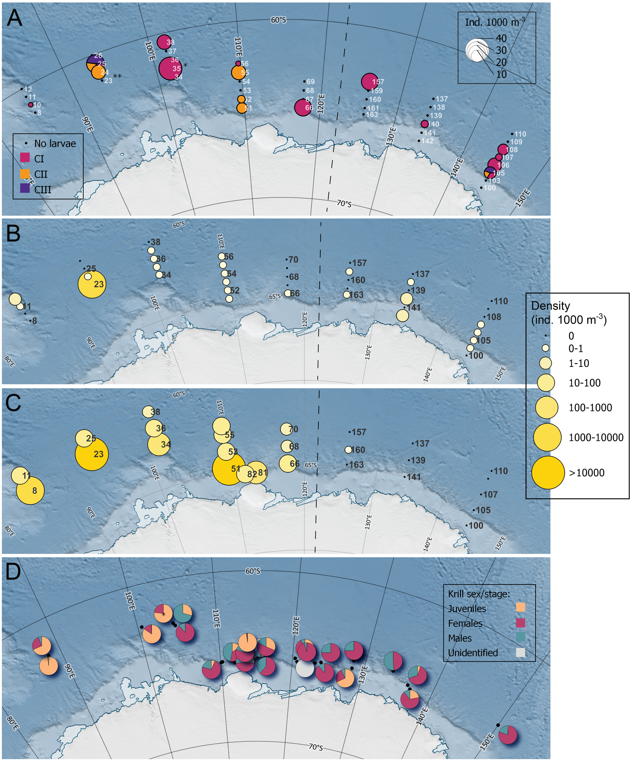
(A) Distribution and density of calyptopis larvae (CI, CII and CIII) of Antarctic krill Euphausia superba, collected using a Rectangular Midwater Trawl (RMT) at predetermined stations in the Indian sector of the Southern Ocean. * indicates the only location were furcilia II larvae were collected. ** indicates the only location were furcilia VI larvae were collected. Furcilia larvae were not taken into account in the depicted densities. (B) Volumetric density (ind. 1000 m-3) of post-larval Antarctic krill per predetermined station collected at 15-200 m depth using the RMT. (C) Volumetric density (ind. 1000m-3) of post-larval Antarctic krill per station collected at 0-2 m depth using the Surface and Under Ice Trawl. Note that not all stations numbers are depicted in maps (B, C). (D) The proportional sex/developmental stage composition of Antarctic krill per targeted RMT station. For visibility, the charts were slightly dodged. The black points show the actual sampling location. The dotted lines indicate the division between Legs 1 and 2.
The number of post-larval krill from the epipelagic layer was very low. The initially calculated average density was 0.27 ind. 1000 m-3, based on RMT 8 catches (Urabe et al., in review)2. Taking into account the large number of post-larval krill collected with the RMT 1 at station 23, the epipelagic contained, on average, 106.81 ± 690.43 ind. 1000 m-3. This includes the small numbers of FVI collected at station 23 (1.6% of the catch). No krill were collected at 19 predetermined RMT stations.
The upper two meters of the water column contained, on average, 2457.02 ± 9031.34 ind. 1000 m-3 krill. This includes FVI larvae which were present in low numbers in the upper surface (1.6% of the population in this stratum). The number of krill collected in the upper two meters of the water column largely exceeded the average number of krill collected using the predetermined RMT (Figures 2B, C). Given the difference in size of the depth layers investigated and to aid comparison with echosounder results, the krill biomass, and both volumetric and areal densities per station are presented for both nets in Table 1. With one exception, the krill occupied the upper surface only in the waters west of 120˚E (Figure 2C).
Table 1
| Station | Volumetric density (ind. 1000 m-3) |
Areal density (ind. 100 m-2) |
Wet mass (g 100 m-2) |
|||
|---|---|---|---|---|---|---|
| RMT | SUIT | RMT | SUIT | RMT | SUIT | |
| 8 | 0 | 3925.21 | 0 | 785.04 | 0 | 119.00 |
| 10 | 0 | 0 | 0 | |||
| 11 | 0.23 | 31.88 | 4.55 | 6.38 | 2.76 | 0.61 |
| 12 | 3.03 | 60.65 | 10.37 | |||
| 23 | 4581.29 | 44144.14 | 91625.73 | 8828.83 | 4437.98 | 882.15 |
| 24 | 0.11 | 2.24 | 0.58 | |||
| 25 | 0 | 43.01 | 0 | 8.60 | 0 | 0.35 |
| 26 | 0 | 0 | 0 | |||
| 34 | 0.21 | 155.56 | 4.28 | 31.11 | 1.00 | 3.14 |
| 35 | 0.37 | 7.35 | 0.44 | |||
| 36 | 0.33 | 23.66 | 6.62 | 4.73 | 1.43 | 0.50 |
| 37 | 0.06 | 1.18 | 0.12 | |||
| 38 | 0 | 5.03 | 0 | 1.01 | 0 | 0.09 |
| 51 | 0.13 | 17898.92 | 2.61 | 3579.78 | 0.13 | 294.82 |
| 52 | 0.27 | 5.40 | 1.30 | |||
| 53 | 0.25 | 45.08 | 5.08 | 9.02 | 2.29 | 0.57 |
| 54 | 0.12 | 2.36 | 3.07 | |||
| 55 | 0.23 | 16.57 | 4.52 | 3.31 | 5.08 | 0.45 |
| 56 | 0.08 | 20.00 | 1.60 | 4.00 | 0.16 | 0.50 |
| 66 | 0.07 | 12.39 | 1.43 | 2.48 | 1.86 | 0.27 |
| 67 | 0 | 0 | 0 | |||
| 68 | 0 | 2.51 | 0 | 0.50 | 0 | 0.04 |
| 69 | 0 | 0 | 0 | |||
| 70 | 0 | 3.14 | 0 | 0.63 | 0 | 0.10 |
| 81 | 101.30 | 20.26 | 2.22 | |||
| 82 | 17.89 | 3.58 | 0.45 | |||
| 100 | 0 | 0 | 0 | 0 | 0 | 0 |
| 103 | 0.04 | 0.80 | 0.4 | |||
| 105 | 0.65 | 0 | 12.93 | 0 | 11.07 | 0 |
| 106 | 0.51 | 10.29 | 5.76 | |||
| 107 | 0.13 | 0 | 2.63 | 0 | 39.49 | 0 |
| 108 | 0 | 0 | 0 | |||
| 109 | 0 | 0 | 0 | 0 | 0 | 0 |
| 110 | 0 | 0 | 0 | 0 | 0 | 0 |
| 137 | 0 | 0 | 0 | 0 | 0 | 0 |
| 138 | 0.22 | 4.33 | 3.03 | |||
| 139 | 0 | 0 | 0 | 0 | 0 | 0 |
| 140 | 2.43 | 48.57 | 68.26 | |||
| 141 | 0 | 0 | 0 | 0 | 0 | 0 |
| 142 | 1.98 | 39.63 | 23.14 | |||
| 157 | 0 | 0 | 0 | 0 | 0 | 0 |
| 159 | 0.07 | 1.37 | 1.09 | |||
| 160 | 0 | 0.74 | 0 | 0.15 | 0 | 0.01 |
| 161 | 0 | 0 | 0 | |||
| 163 | 0.06 | 0 | 1.16 | 0 | 0.7 | 0 |
Volumetric density, areal densities and wet mass of Antarctic krill (Euphausia superba) per predetermined station collected in the 15-200 m depth layer using RMT (Rectangular Midwater Trawl) and the 0-2 m depth layer using SUIT (Surface and Under Ice Trawl).
It should be noted that post-larval krill densities were derived from the RMT 8 net, except for station 23 where krill were only collected in the RMT 1 net. Densities may include small numbers of furcilia VI, sizes of which overlapped with those of juveniles.
3.2 Developmental stage distribution
At 21 predetermined RMT stations 10 or less individuals were caught. At only four predetermined RMT stations there were a sufficient number of individuals to establish a length-frequency distribution. At two of these stations, located on the two most western transect lines of the sampling area, the catch was dominated by juveniles (Supplementary Figure S1). At two stations east of 130˚E one catch (station 140) was dominated by gravid females (F3D) and adult males (M3B), while the other (station 142) was dominated by sub-adult females and males (Supplementary Figure S1).
Krill were collected during 36 target RMT hauls at 26 different stations. Of these hauls, 28 contained more than 20 individuals which were used for length-frequency distribution. The size structure of krill sampled varied across the survey area (Figure 2D). The length-frequency distribution of target hauls showed unimodal and bimodal peaks (Figures 3, 4). With some exceptions, the first peak usually consisted of juveniles and sub-adults males (M2A) and females (F2), while the second peak was often dominated by gravid females (F3D) and adults males (M3B). Some samples or peaks consisted of adult, non-gravid females (F3B and F3C) and late-stage sub-adult males (M2B and M2C). Small numbers of spent females (F3E) occurred only occasionally. Juveniles dominated the catches in 9 out of 16 measured stations conducted west of 120 ˚E, which all sampled the upper 15-50 m of the water column (Figures 2D, 3; Supplementary Table S4). East of 120 ˚E, juveniles dominated at 2 out of 12 measured stations, one that sampled the upper 15-50 m and one that sampled below 300 m deep (Figure 4). Sub-adult and adult female and male krill occurred throughout the water column (Figures 3, 4).
Figure 3

Length and stage distribution of Antarctic krill (Euphausia superba) at target RMT stations from trawls conducted west of 120 ˚E where >20 individuals could be measured. Trawls were conducted between 15 and 50 m depth (light grey headings), or between 50 and 75 m depth (grey headings). At some stations, multiple aggregations were collected during a single tow, indicated by plots with the same station number.
Figure 4

Length and stage distribution of Antarctic krill (Euphausia superba) at target RMT stations from trawls conducted east of 120 ˚E where >20 individuals could be measured. Trawls were conducted between 15 and 50 m depth (light grey headings) or between 200 and 600 m depth (dark grey headings). At some stations, multiple aggregations were collected during a single tow, indicated by plots with the same station number.
The vast majority of, mainly post-larval, krill collected in the upper two meters of the water column were juveniles (92%), followed by early sub-adult females (F2B, 2.7%) and males (M2A1, 2.1%). The other stages were present in low numbers (Supplementary Table S5). Length-frequency distributions were similar across stations. An average length-frequency is shown in Figure 5. Late gravid (F3D) and spent (F3E) females were completely absent in the surface waters.
Figure 5
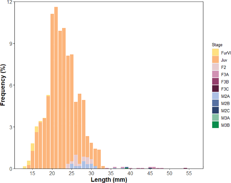
Average length-frequency distribution of Antarctic krill (Euphausia superba) in the upper two meters of the water column collected using the Surface and Under Ice Trawl.
3.3 Krill size comparison
The average size of juveniles in the SUIT hauls ranged between 17.8 and 23.8 mm per station (Figure 6A; Supplementary Table S6). Although there were significant differences between some stations ((F13,616269 = 1264, p = < 0.0001), differences were not consistently higher or lower with seasonal progression (Figure 6A). The average size of juveniles in the target RMT hauls ranged from 21.1 to 36.3 mm, which was much a wider range compared to the average size of juveniles collected in the surface using the SUIT. Generally, the average size of juveniles per target station with >20 individuals increased as time progressed, but showed smaller krill again at station 64 after which size proceeded to increase with the progression of time (Figure 6B). Juveniles were significantly larger at stations 32 and 44 compared to station 64 (F12, 980 = 219.9, p < 0.0001, Tukey HSD: p <0.006), although sampling was conducted five and eight days earlier, respectively. Stations 18 to 44 were conducted north of 64˚S, in the vicinity of the ice edge. At these stations, the average size of juvenile increased from 21.1 mm to 27.7 mm in 7 days. The average size of two aggregations sampled at station 18 (averaging 21.1 and 24.1 mm) were significantly different from each other (F12, 980 = 219.9, p < 0.0001, Tukey HSD: p <0.0001). Stations 64 onwards were conducted near the shelf break (Figure 6B). The average size of the juveniles collected at these stations increased from 23.6 to 36.3 mm in 48 days. The juveniles at station 515 were, on average, significantly larger compared to juveniles at all other stations (F12, 980 = 219.9, p < 0.0001, Tukey HSD: p < 0.002).
Figure 6
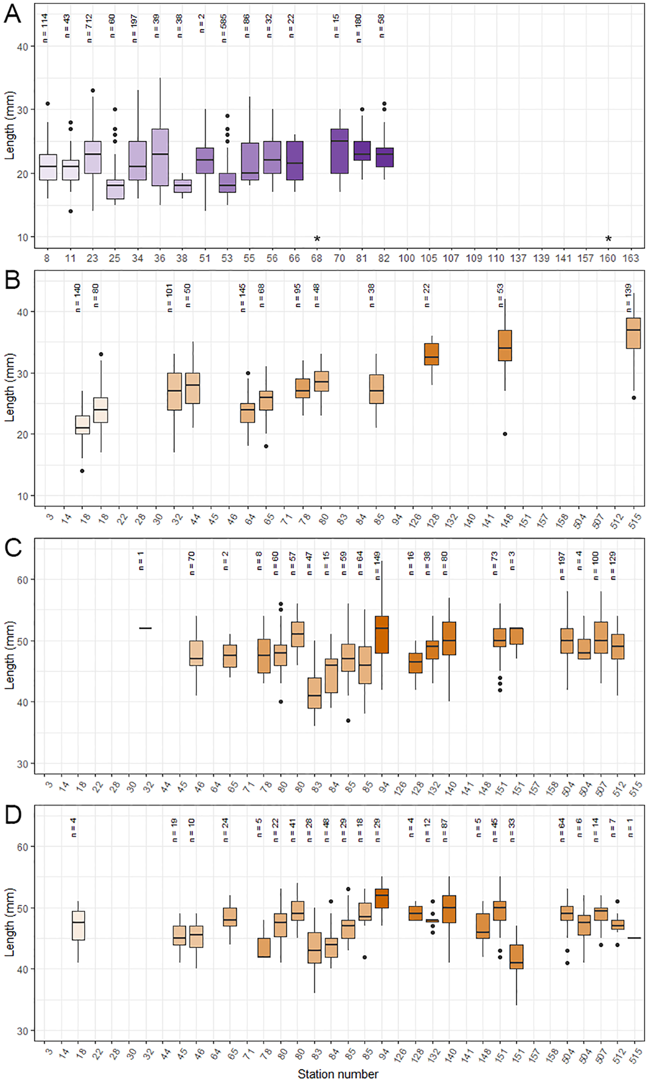
Average size per station of (A) juvenile Antarctic krill (Euphausia superba) collected in the 0-2 m depth layer using SUIT, (B) juvenile krill collected at target RMT hauls, (C) gravid females (F3D) collected at target RMT hauls and (D) adult male (M3B) collected at target RMT hauls. At some stations, multiple aggregations were collected during a single tow, indicated by the same station number. Station numbers are ascending with time, so the x-axis reflects seasonal progression. The colour gradients represent longitude, with colours transitioning from light to dark going from west to east. n is the number of individuals measured. The horizontal black lines show the median length in a station. The upper and lower limits of the squares indicated the 25th and 75th percentile. The upper and lower limits of the vertical line indicate the minimum and maximum length of juveniles in a station. Dots represent the true minimum and maximum lengths, but are numerically distant (percentile ± the interquartile range) from the other data points and therefore considered outliers. * indicates stations with low number of Antarctic krill for which no length measurements could be established; blank stations totally lacked krill.
There were no distinct patterns in the average size of gravid females (F3D) in the target RMTs (Figure 6C). Gravid females at station 83 were significantly smaller than the ones at all other stations (F10,949 = 36.67, p = < 0.0001, Tukey p < 0.0001). The gravid females of stations 46, 80 and 85 were significantly smaller than the ones at some other stations (F10,949 = 36.67, p = < 0.0001, Tukey p < 0.04). Two gravid female aggregations collected during a single RMT tow at station 80 differed significantly from each other in average size (F10,949 = 36.67, p = < 0.0001, Tukey p < 0.0001). For adult males (M3B) some increase in average size seems to occur over periods of time, but this was not as consistent as with the juveniles and more variation was present (Figure 6D). Adults males at stations 83, 84 and 151 were significantly smaller than individuals at all other stations, except for from station 45 and each other (F12,474 = 42.01, p = < 0.0001, Tukey p < 0.001). Two adult male aggregations collected during a single RMT tow at station 151 differed significantly from each other in average size (F12,474 = 42.01, p = < 0.0001, Tukey p < 0.0001).
4 Discussion
4.1 Krill distributional patterns
Our study showed that a significant part of the krill population resided in the upper surface of the water column, which is not sampled by conventional trawls or echosounders. Although such upper-surface dwelling of mainly juveniles has been suspected (e.g. Jarvis et al., 2010; Atkinson et al., 2012), our study provides a quantitative estimate of density and length-frequency distribution of this part of the krill stock in the Indian sector of the Southern Ocean. The actual part of the stock in the undersampled surface layer may even be larger than the stock size estimated by SUIT, since the densities in the 0-2 m depth layer will likely gradually decrease to the densities as found below 15 m (Schaafsma et al., 2024).
The number of krill in the epipelagic layer, estimated using predetermined RMT catches, was low compared to the numbers encountered in the nets during BROKE (Nicol et al., 2000b). In contrast to the net data, echosounder data collected during our survey suggests that the total biomass of krill in the 20-200 m depth stratum was similar during KY1804 and BROKE (Pauly et al., 2000; Abe et al., 2023). Potential reasons for a lack of krill in the predetermined RMT hauls can be net avoidance or, more likely, the concentration of krill in aggregations, which were simply not encountered enough in the sampling design. This is a common caveat in net-based sampling of schooling or swarming species (Mackintosh, 1973; Watkins, 2000; Nicol and Brierley, 2010).
The echosounder estimates of areal biomass densities reported from our survey showed that the horizontal distribution of krill seemed to vary between the areas west and east of 120˚E (Abe et al., 2023). In the west, echosounder data found krill relatively evenly distributed despite variation in latitude among transect lines sampled, with a peak in krill density at the transect furthest west (80˚E) (Abe et al., 2023). In the east, highest densities seemed to occur close to the shelf break, south of the southern boundary of the Antarctic Circumpolar Current, with the exception of the echosounder transect furthest east (150˚E) where high densities occurred along the entire transect (Abe et al., 2023). This distribution pattern is similar to those found in January to March during the Discovery expeditions (Mackintosh, 1973) and the BROKE expedition (Nicol et al., 2000b).
During BROKE, the differences in horizontal post-larval krill distribution between west and east were attributed to the more southward intrusion of warmer water in the eastern side of the sampling area, resulting from the southeastward flow of the ACC in the region, constraining the krill habitat closer to the coast (Bindoff et al., 2000; Nicol et al., 2000b). Such a geographic east-west difference in surface temperature was even more pronounced during the KY1804 expedition (Urabe et al., in review; Yamazaki et al., 2024). The temperature at the western side of the sampling area was generally between 0 and 1°C, with a few exceptions at the southernmost stations of certain transects were temperatures below 0°C occurred. At the eastern side of the sampling area, negative temperatures, down to -1.5°C, were found at the southern half of the transects, while temperatures in the northern half of the transects were generally higher than 1°C. Other environmental variables may have contributed to differences in distribution. The chlorophyll a concentration during our study was, on average, somewhat higher in the east than it was in the west, and retreating sea ice occurred more northernly on the western side of the sampling area while it already retreated to the vicinity of the shelf or beyond on the eastern side (Figure 1; Urabe et al., in review; Yamazaki et al., 2024).
The temperature differences between both sides of the sampling area, as well as the wider sea-ice extent resulting from transportation of formed sea ice found in the west, may be attributed to a series of subgyres, with several warmer water currents flowing southward and colder waters from the ASC flowing northward, in the region between 80 and 130˚E (Yamazaki et al., 2020; Hirano et al., 2021). The gyres are united with the ACC that travels in close proximity to the continental shelf (Yamazaki et al., 2020). In concurrence with conclusions from previous studies, differences in the population structure of post-larval krill between the areas west and east of 120˚E are likely a result of a combination of seasonality and physical factors, including time of sea-ice cover. The time gap between sampling in Leg 1 and 2 may have had an additional influence on distribution patterns. Growth and development may alter the vertical distribution of krill because the trade-off between food availability, energy budget and predation risk changes (Lampert, 1989; Quetin et al., 1996).
4.2 Krill size and developmental stage distribution
The number of individuals that could be measured from the predetermined RMT hauls was generally too small to obtain a reliable length-frequency distribution, which limited the analysis of temporal and spatial patterns in the distribution of different life stages in the 15-200 m depth layer. Target RMT hauls were mainly conducted to investigate the composition of acoustically detected targets and were performed opportunistically across a variety of locations and depths. These data on the horizontal and vertical distributions are thus, inherently biased (Watkins, 1999; Nicol et al., 2000b; Abe et al., 2023). However, combined with the SUIT net and acoustics, they can provide some information on distribution patterns of different life stages.
Target RMT hauls indicated that juveniles were often more dominant in the krill catches from the western side of the sampling area compared to the eastern side of the sampling area during our study (Figures 2D, 3, 4), which was similar to the findings of BROKE (Nicol et al., 2000b). This dominance of juveniles mainly occurred in the upper 15-50 m of the water column, with the exception of one deeper station in the eastern side of the sampling area. This corresponds with the findings from the surface water sampling which provided further evidence that juveniles remained close to the surface in this region, as the SUIT catches consisted mainly of juveniles. This upper surface dwelling occurred on the western side of the sampling area, and almost no krill was encountered in this stratum in the east (Figure 2C).
Patterns in horizontal distribution were only observed for post-larval krill, and perhaps for late stage furcilia on the verge of developing into juveniles. Predetermined RMT 1 hauls indicated that, during KY1804, younger calyptopis larval krill were distributed more evenly throughout the sampling area with densities ranging from 1.5 to 37.6 ind. 1000 m-3 (Figure 2A; Matsuno et al., in review)3. CI larvae were present in relatively small numbers throughout the sampling area during our survey, while stations with CII and CIII larvae occurred in various regions. This is different from results from BROKE, where very high larval densities were encountered in the eastern part of the sampling area with a mean density of 3186 ind. 1000 m-3, and numbers were much lower west of 120˚E (Nicol et al., 2000b). Calyptopis stages were found throughout the survey area during BROKE, while early furcilia stages were mainly found in the east, which was attributed to seasonal progression (Nicol et al., 2000b).
Based on predetermined RMT 1 hauls, the CI larvae were encountered between 17 December and 13 February during our survey, indicating that spawning occurred between 17 November and 31 January, assuming that the developmental time of CI larvae is between 13 and 30 days depending on conditions that may influence development such as temperature (Ikeda, 1984; Jia et al., 2014). CIII larvae occurred from 21 December to 31 January, indicating spawning potentially between 19 October and 18 December, assuming a developmental time between 40 and 63 days (Ikeda, 1984; Spiridonov, 1995; Jia et al., 2014). Considering the low numbers of larvae, the presence of gravid females in the target RMT hauls throughout the survey area and the almost total absence of spent females in these catches, this timing suggests that spawning occurred quite early (Spiridonov, 1995) and had not yet peaked. This could explain the low density of larvae compared to the findings of BROKE, which was conducted later in the season and during which high numbers in the east were mainly collected in the whole of March (Nicol et al., 2000b). During BROKE, gravid females were mainly found in targeted trawls conducted in the region west of 120˚E while spent females were mainly found in the east, which could also be attributed to seasonal progression (Nicol et al., 2000b).
Results from target RMTs did not indicate a distinct temporal pattern in the size of gravid females indicating that their size remained similar throughout the survey (Figure 6C). This corresponds to earlier findings and can be due to a lack of growth because of energy investment in reproduction (Nicol et al., 2000b). Also similar to findings of previous studies (Nicol et al., 2000b), adult males showed some growth, although this was not consistent throughout the study area (Figure 6D). This could be a result of different populations sampled, a reflection of differences in feeding conditions or due to an increased energy investment in reproduction.
The size of juvenile krill twice increased with time in the 15-50 m depth layer sampled during target RMT hauls (Figure 6B). Assuming that these juveniles originate from two spawning populations or spawning events, and their increase in size comes from natural growth, the two groups would have been growing with 0.94 mm day-1 in the more northern stations and with 0.21 mm day-1 at the more southern stations, located near the shelf break. Although this latter rate can be considered realistic, the former growth rate is much higher than maximum growth rates recorded (Atkinson et al., 2006; Tarling et al., 2006). It, therefore, seems likely that, at least in the part of the sampling area where transects were located north of ~62˚S, juveniles originated from multiple spawning events. Alternatively, the juveniles may have originated from various locations, which could have resulted in different growth rates due to variable environmental conditions experienced.
The juveniles in the upper surface were all relatively small and their size remained similar over time and space, in contrast to the increasing size of juveniles from the target RMTs over time (Figure 6A). This may, again indicate various origins of the juveniles collected, perhaps resulting from the series of subgyres found in the area (Yamazaki et al., 2020). It may also indicate a small scale, gradual change in vertical distribution range within this developmental stage, with the vertical distribution range increasing with increasing size. Such a small-scale change in distribution was also suggested for furcilia larvae/age class 0 juveniles during winter (Schaafsma et al., 2016). Although these were caught under ice and their relationship with the environment is likely very different, such changes may be a result of similar mechanisms, such as saving energy by passive sinking, the speed of which increases with increasing size (Kils, 1982). However, further research is necessary to test such a hypothesis, especially since a previous study indicated that the vertical distribution of krill recruits (age 1+) depends on season (Pakhomov, 1995). In addition, it should be noted that krill were only collected in the surface during Leg 1, while length comparisons encompassed both legs for the target RMT catches.
4.3 Consequences of undersampling of the surface
The previously assumed distributional patterns of particularly juveniles may have been based on an incomplete picture. For example, several studies suggested a trend of younger individuals remaining south of the shelf break during summer, while older animals reside further offshore, north of the shelf break (Siegel, 1988; Lascara et al., 1999; Nicol et al., 2000b; Atkinson et al., 2008). However, the potential distribution in the upper surface waters was not taken into account in these studies. Knowledge on the presence of krill in the upper surface would aid in understanding smaller-scale and larger-scale distribution processes. For example, the aforementioned migration of different life-stages and the potential relation with oceanographic features such as gyres, that might aid in moving on- and off-shelf. Another example are circumpolar advection patterns that are expected to be greatly influenced by behavioural patterns (Hofmann et al., 1998; Murphy et al., 2004; Atkinson et al., 2008).
Length-frequency distributions of krill are often used to calculate an estimated recruitment value, which is used as a parameter in management models (Butterworth et al., 1991; Constable and de la Mare, 1996) and to assess the success of spawning in a certain year (Watkins, 1999). Because of the small numbers of krill collected in the predetermined RMT hauls, it was not possible to make an estimation for recruitment that is comparable to numbers from previous studies. Results from the SUIT sampling indicate that recruitment indices can be biased because obtained data is not fully representative of the entire stock due to the spatial segregations of life stages (Siegel and Loeb, 1995).
4.4 Knowledge gaps and future research
More information on the potential presence of DVM of krill is desirable to fully understand the consequences of the undersampling of the surface layer on biomass estimates and recruitment indices, as it cannot be excluded that surface krill move into water layers within the detection range of echosounders during certain times of the day. Analysis of the SUIT data provided some indication that DVM of E. superba was occurring during the survey, but the number of day and night hauls was unevenly distributed throughout the sampling area, potentially biasing comparison (Schaafsma et al., 2024). In addition, no obvious DVM patterns was found in the echosounder data (Abe et al., 2023). Thus, although this could be a result of krill performing only a shallow DVM, data collected during the survey does not provide conclusive evidence on the presence or absence of DVM. A similar conclusion was drawn from analyses performed on data collected during BROKE (Pauly et al., 2000).
It is important to note that very few krill was collected in the upper surface in the western side of the sampling area (Figures 2B, 6A). Therefore, it would be useful to increase knowledge on when and where juvenile krill accumulate in this layer, and to investigate the potential relationship with environmental and/or biological variables. This includes the distribution of juveniles in ice-covered waters, as sea ice was still present in the area at the time of sampling and is known to affect the distribution of various life stages (Flores et al., 2012). Such information would help to understand if a sampling bias occurs when parts of the potential krill habitat are not sampled (Quetin and Ross, 2003), and to assess if estimates of calculated recruitment indices are representative. For example, an underestimation of recruitment in the Antarctic Peninsula region was suspected in the Palmer LTER study (Quetin and Ross, 2003), which might be explained by undersampling of surface juveniles. In addition, although recruitment has been positively correlated with various aspects of sea-ice dynamics such as late sea-ice retreat (Siegel and Loeb, 1995) or an August maximum sea-ice extent (Quetin and Ross, 2003), a better understanding of relationships between successful spawning years and environmental variables or changes in transport mechanisms may have been hampered by a inaccurate estimation of the density of krill per year class (Siegel and Loeb, 1995; Watkins, 1999). Such knowledge would aid in understanding of natural variability of krill stocks (Siegel and Loeb, 1995) and the potential consequences of climate warming (Quetin and Ross, 2003).
More knowledge regarding the distribution of krill in the upper surface may also aid in understanding the distribution of top predator species. For example, a relationship between the distribution of 13-34 mm krill and the foraging grounds of humpback whales Megaptera novaeangliae has been demonstrated in the Antarctic Peninsula region (Santora et al., 2010). During our survey, humpback whales were also more abundant in the western side of the sampling area compared to the eastern side (Hamabe et al., 2024). In addition, depending on the method used, krill consumption by humpback whales exceeded the total krill biomass as established by echosounder data (Abe et al., 2023; Hamabe et al., 2024). This might be explained by the exclusion of a part of the krill stock in the biomass estimate, although juveniles would contribute less to total krill biomass compared to the same number of adults. A lack of knowledge on the distribution of krill in the upper surface may also explain discrepancies between stomach contents and net samples, as found in diet studies such as for the minke whale Balaenoptera acutorostrata (Ichii and Kato, 1991). The diet of this species has been found to regularly contain large proportions of one-year-old juvenile krill depending on the region of occurrence (Ichii and Kato, 1991; Ichii et al., 1998).
Statements
Data availability statement
The raw data supporting the conclusions of this article will be made available by the authors, without undue reservation.
Ethics statement
The manuscript presents research on animals that do not require ethical approval for their study.
Author contributions
FS: Conceptualization, Formal analysis, Investigation, Methodology, Project administration, Visualization, Writing – original draft. RD: Formal analysis, Investigation, Methodology, Writing – review & editing. KM: Formal analysis, Funding acquisition, Supervision, Writing – review & editing. RS: Formal analysis, Investigation, Writing – review & editing. SD: Investigation, Writing – review & editing. MR: Investigation, Writing – review & editing. HS: Investigation, Supervision, Writing – review & editing. RM: Investigation, Supervision, Writing – review & editing. JF: Conceptualization, Funding acquisition, Writing – review & editing, Methodology. HM: Conceptualization, Funding acquisition, Investigation, Methodology, Project administration, Supervision, Writing – review & editing.
Funding
The author(s) declare that financial support was received for the research, authorship, and/or publication of this article. The KY1804 survey was supported by the Institute of Cetacean Research, the Japan Fisheries Research and Education Agency, and the Fisheries Agency of Japan. Antarctic research by Wageningen Marine Research is commissioned by the Netherlands Ministry of Agriculture, Nature and Food Quality (LNV) which funded this research under its Statutory Research Task Nature & Environment WOT-04-009-047.04.
Acknowledgments
We are very grateful to the officers, crew, and colleague researchers onboard RV Kaiyo-maru for their indispensable assistance with the biological sampling. Thanks to André Meijboom and Oliver Bittner (Wageningen Marine Research) for assistance with SUIT krill sample analysis, to Giulia Castellani (Alfred Wegener Institute) for processing ADCP data, and to Michiel van Dorssen (M. van Dorssen Metaalbewerking) for technical support using SUIT.
Conflict of interest
The authors declare that the research was conducted in the absence of any commercial or financial relationships that could be construed as a potential conflict of interest.
Publisher’s note
All claims expressed in this article are solely those of the authors and do not necessarily represent those of their affiliated organizations, or those of the publisher, the editors and the reviewers. Any product that may be evaluated in this article, or claim that may be made by its manufacturer, is not guaranteed or endorsed by the publisher.
Supplementary material
The Supplementary Material for this article can be found online at: https://www.frontiersin.org/articles/10.3389/fmars.2024.1411130/full#supplementary-material
Footnotes
1.^Murase, H., Abe, K., Schaafsma, F. L., and Katsumata, K. Overview of the multidisciplinary ecosystem survey in the eastern Indian sector of the Southern Ocean (80–150°E) by the Japanese research vessel Kaiyo-maru in the 2018–19 austral summer (KY1804 survey). Progr. Oceanogr.
2.^Urabe, I., Matsuno, K., Sugioka, R., Driscoll, R., Driscoll, S., Schaafsma, F. L., et al. Spatio-temporal changes in the macrozooplankton community in the eastern Indian sector of the Southern Ocean during austral summer: comparison between 1996 and 2018/2019. Progr. Oceanogr.
3.^Matsuno, K., Sugioka, R., Maeda, Y., Driscoll, R., Schaafsma, F. L., Yamaguchi, A., et al. Spatial changes in the mesozooplankton and population structure of dominant species in the eastern Indian sector of the Southern Ocean during austral summer 2018/2019. Progr. Oceanogr.
References
1
Abe K. Matsukura R. Yamamoto N. Amakasu K. Nagata R. Murase H. (2023). Biomass of Antarctic krill (Euphausia superba) in the eastern Indian sector of the Southern Ocean (80–150°E) in the 2018–19 austral summer. Progr. Oceanogr.218, 103107. doi: 10.1016/j.pocean.2023.103107
2
Atkinson A. Nicol S. Kawaguchi S. Pakhomov E. Quetin L. Ross R. et al . (2012). Fitting Euphausia superba into Southern Ocean food-web models: a review on data sources and their limitations. CCAMLR Sci.19, 219–245.
3
Atkinson A. Shreeve R. S. Hirst A. G. Rothery P. Tarling G. A. Pond D. W. et al . (2006). Natural growth rates in Antarctic krill (Euphausia superba): II. Predictive models based on food, temperature, body length, sex, and maturity stage. Limnol. Oceanogr.51, 973–987. doi: 10.4319/lo.2006.51.2.0973
4
Atkinson A. Siegel V. Pakhomov E. A. Rothery P. Loeb V. Ross R. M. et al . (2008). Oceanic circumpolar habitats of Antarctic krill. Mar. Ecol. Prog. Ser.362, 1–8. doi: 10.3354/meps07498
5
Baker A. D. C. Clarke M. R. Harris M. J. (1973). The N.I.O. combination net (RMT 1 + 8) and further developments of rectangular midwater trawls. J. Mar. Biol. Assoc. UK53, 167–184. doi: 10.1017/S0025315400056708
6
Bindoff N. L. Rosenberg M. A. Warner M. J. (2000). On the circulation and water masses over the Antarctic continental slope and rise between 80 and 150˚E. Deep-Sea Res. II47, 2299–2326. doi: 10.1016/S0967-0645(00)00038-2
7
Bryantsev V. A. Kovalenko L. A. Bibik V. A. (1991). “Hydrometeorological bases for forecasting of the Antarctic krill, Euphausla superba Dana, distribution and biomass in the Cooperation Sea,” in Document WG-KRILL-91/43 (CCAMLR, Hobart, Australia), 1–6.
8
Butterworth D. S. Punt A. E. Basson M. (1991). “A simple approach for calculating the potential yield of krill from biomass survey results,” in Selected Scientific Papers (SC-CAMLR-SSPI8) (CCAMLR, Hobart, Australia), 207–217.
9
CCAMLR (2021). Available online at: https://www.ccamlr.org/en/fisheries/krill (Accessed 11 December 2023).
10
Constable A. J. de la Mare W. K. (1996). A generalized model for evaluating yield and the long-term status of fish stocks under conditions of uncertainty. CCAMLR Sci.3, 31–54.
11
Cox M. J. Macauley G. Brasier M. J. Burns A. Johnson O. J. King R. et al . (2022). Two scales of distribution and biomass of Antarctic krill (Euphausia superba) in the eastern sector of the CCAMLR Division 58.4.2 (55˚E to 80˚E). PloS One17, e0271078. doi: 10.1371/journal.pone.0271078
12
Everson I. Bone D. G. (1986). Effectiveness of the RMT8 system for sampling krill (Euphausia superba) swarms. Polar Biol.6, 83–90. doi: 10.1007/BF00258257
13
Flores H. Hunt B. P. V. Kruse S. Pakhomov E. A. Siegel V. Van Franeker J. A. et al . (2014). Seasonal changes in the vertical distribution and community structure of Antarctic macrozooplankton and micronekton. Deep-Sea Res. I84, 127–141. doi: 10.1016/j.dsr.2013.11.001
14
Flores H. Van Franeker J. A. Siegel V. Haraldsson M. Strass V. Meesters E. H. W. G. et al . (2012). The association of Antarctic krill Euphausia superba with the under-ice habitat. PloS One7, e31775. doi: 10.1371/journal.pone.0031775
15
Fraser F. C. (1936). On the development and distribution of the young stages of krill (Euphausia superba). Discovery Rep.14, 3–190. doi: 10.5962/bhl.part.3886
16
Hamabe K. Miyashita T. Nagata R. Sasaki H. Murase H. (2024). Abundance of humpback whales in the eastern Indian sector of the Southern Ocean in 2018/19 using opportunistic sighting survey data with a note on the occurrence of other cetaceans. Progr. Oceanogr.226, 103296. doi: 10.1016/j.pocean.2024.103296
17
Hill S. L. Murphy E. J. Reid K. Trathan P. N. Constable A. J. (2006). Modelling Southern Ocean ecosystems: krill, the food-web, and the impacts of harvesting. Biol. Rev. Cam. Philos. Soc81, 581–608. doi: 10.1017/S1464793106007123
18
Hirano D. Mizobata K. Sasaki H. Murase H. Tamura T. Aoki S. (2021). Poleward eddy-induced warm water transport across a shelf break off Totten Ice Shelf, East Antarctica. Commun. Earth Environ.2, 153. doi: 10.1038/s43247-021-00217-4
19
Hofmann E. E. Klinck J. M. Locarnini R. A. Fach B. A. Murphy E. J. (1998). Krill transport in the Scotia Sea and environs. Antar Sci.10, 406–415. doi: 10.1017/S0954102098000492
20
Hosie G. W. Ikeda T. Stolp M. (1988). Distribution, abundance and population structure of the Antarctic krill (Euphausia superba) in the Prydz Bay region, Antarctica. Polar Biol.8, 213–224. doi: 10.1007/BF00443453
21
Ichii T. Kato H. (1991). Food and daily food-consumption of Southern minke whales in the Antarctic. Polar Biol.11, 479–487. doi: 10.1007/BF00233083
22
Ichii T. Shinohara N. Fujise Y. Nishiwaki S. Matsuoka K. (1998). Interannual changes in body fat condition index of minke whales in the Antarctic. Mar. Ecol. Progr. Ser.175, 1–12. doi: 10.3354/meps175001
23
Ikeda T. (1984). Development of the larvae of the Antarctic krill (Euphausia superba Dana) observed in the laboratory. J. Exper. Mar. Biol. Ecol.75, 107–117. doi: 10.1016/0022-0981(84)90175-8
24
Jarvis T. Kelly N. Kawaguchi S. Van Wijk E. Nicol S. (2010). Acoustic characterisation of the broad-scale distribution and abundance of Antarctic krill (Euphausia superba) off East Antarctica (30-80˚E) in January-March 2006. Deep-sea Res. II57, 916–933. doi: 10.1016/j.dsr2.2008.06.013
25
Jia Z. Virtue P. Swadling K. M. Kawaguchi S. (2014). A photographic documentation of the development of Antarctic krill (Euphausia superba) from egg to early juvenile. Polar Biol.37, 165–179. doi: 10.1007/s00300-013-1420-7
26
Kawaguchi S. Nicol S. Virtue P. Davenport S. R. Casper R. Swadling K. M. et al . (2010). Krill demography and large-scale distribution in the Western Indian Ocean sector of the Southern Ocean (CCAMLR Division 58.4.2) in Austral summer of 2006. Deep-Sea Res. II57, 934–947. doi: 10.1016/j.dsr2.2008.06.014
27
Kils U. (1982). Swimming behaviour, swimming performance and energy balance of Antartic krill, Euphausia superba. Biomass Sci. Ser.3, 1–121.
28
Kinzey D. Watters G. M. Reiss C. S. (2019). Estimating recruitment variability and productivity in Antarctic krill. Fish. Res.217, 98–107. doi: 10.1016/j.fishres.2018.09.027
29
Kirkwood J. M. (1982). A Guide to the Euphausiacea of the Southern Ocean (Kingston: ANARE Research Notes 1, Australian Antarctic Division), 4.
30
Lampert W. (1989). The adaptive significance of diel vertical migration of zooplankton. Funct. Ecol.3, 21–27. doi: 10.2307/2389671
31
Lascara C. M. Hofmann E. E. Ross R. M. Quetin L. B. (1999). Seasonal variability in the distribution of Antarctic krill, Euphausia superba, west of the Antarctic Peninsula. Deep-Sea Res. I46, 951–984. doi: 10.1016/S0967-0637(98)00099-5
32
Mackintosh N. A. (1973). Distribution of post-larval krill in the Antarctic. Discovery Rep.36, 95–156.
33
Makarov R. R. Denys C. J. (1981). Stages of sexual maturity of Euphausia superba Dana. Biomass Handb.11, 2–13.
34
Marr J. (1962). The natural history and geography of the Antarctic krill (Euphausia superba Dana). Discovery Rep.32, 37–123.
35
Matsuoka K. Skoglund A. Roth G. De Pomereu J. Griffiths H. Headland R. et al . (2021). QuAntarctica, an integrated mapping environment for Antarctica, the Southern Ocean, and sub-Antarctic islands. Environ. Modell. Software140, 105015. doi: 10.1016/j.envsoft.2021.105015
36
Mauchline J. (1980). The biology of mysids and euphausiids. Adv. Mar. Biol.18, 681.
37
Methot R. D. (1986). Frame trawl for sampling pelagic juvenile fish. California Coop. Ocean. Fish. Investig. Rep.27, 267–278.
38
Miller D. G. M. (1985). The South African SIBEX I cruise to the Prydz Bay regio. S. Afr. J. Antarct. Res.15, 33–41.
39
Miquel J. C. (1991). Distribution and abundance of post-larval krill (Euphausia superba Dana) near Prydz Bay in summer with reference to environmental conditions. Antarc. Sci.2, 279–292. doi: 10.1017/S0954102091000342
40
Murphy E. J. Thorpe S. E. Watkins J. L. Hewitt R. (2004). Modeling the krill transport pathways in the Scotia Sea: spatial and environmental connections generating the seasonal distribution of krill. Deep-Sea Res. II51, 1435–1456. doi: 10.1016/j.dsr2.2004.06.019
41
Nicol S. Brierley A. S. (2010). Through a glass less darkly—New approaches for studying the distribution, abundance and biology of Euphausiids. Deep-Sea Res. II57, 496–507. doi: 10.1016/j.dsr2.2009.10.002
42
Nicol S. Kitchener J. King R. Hosie G. de la Mare W. K. (2000b). Population structure and condition of Antarctic krill (Euphausia superba) of East Antarctica (80-150˚E) during the Austral summer of 1995/1996. Deep-Sea Res. II47, 2489–2517. doi: 10.1016/S0967-0645(00)00033-3
43
Nicol S. Pauly T. Bindoff N. L. Strutton P. G. (2000a). BROKE” a biological/oceanographic survey of the coast of East Antarctica (80-150˚E) carried out in January-March 1996. Deep-Sea Res. II47, 2281–2298. doi: 10.1016/S0967-0645(00)00026-6
44
Pakhomov E. A. (1995). Demographic studies of Antarctic krill Euphausia superba in the Cooperation and Cosmonaut Seas (Indian sector of the Southern Ocean). Mar. Ecol. Progr. Ser.119, 45–61. doi: 10.3354/meps119045
45
Pakhomov E. A. (2000). Demography and life cycle of Antarctic krill, Euphausia superba, in the Indian sector of the Southern Ocean: long-term comparison between coastal and open-ocean regions. Can. J. Fish. Aq. Sci.57, 68–90. doi: 10.1139/f00-175
46
Pauly T. Nicol S. Higginbottom I. Hosie G. Kitchener J. (2000). Distribution and abundance of Antarctic krill (Euphausia superba) off East Antarctic (80-150˚E) during the austral summer of 1995/1996. Deep-Sea Res. II47, 2465–2488. doi: 10.1016/S0967-0645(00)00032-1
47
Piccolin F. Pitzschler L. Biscontin A. Kawaguchi S. Meyer B. (2020). Circadian regulation of diel vertical migration (DVM) and metabolism in Antarctic krill Euphausia superba. Sci. Rep.10, 16796. doi: 10.1038/s41598-020-73823-5
48
Quetin L. B. Ross R. M. (2003). Episodic recruitment in Antarctic krill Euphausia superba in the Palmer LTER study region. Mar. Ecol. Progr. Ser.259, 185–200. doi: 10.3354/meps259185
49
Quetin L. B. Ross R. M. Frazer T. K. Haberman K. L. (1996). Factors affecting distribution and abundance of zooplankton, with an emphasis on Antarctic krill, Euphausia superba. Antarc. Res. Ser.70, 357–371. doi: 10.1029/AR070p0357
50
R Core Team (2022). R: A language and environment for statistical computing (Vienna, Austria: R Foundation for Statistical Computing).
51
Roe H. S. J. Shale D. M. (1979). A new multiple rectangular midwater trawl (RMT 1 + 8M) and some modifications to the institute of oceanographic sciences' RMT 1 + 8. Mar. Biol.50, 283–288. doi: 10.1007/BF00394210
52
Santora J. A. Reis C. S. Loeb V. J. Veit R. R . (2010). Spatial association between hotspots of baleen whales and demographic patterns of Antarctic krill Euphausia superba suggests size-dependent predation. Mar. Ecol. Progr. Ser.405, 255–269. doi: 10.3354/meps08513
53
Schaafsma F. L. David C. Pakhomov E. A. Hunt B. P. V. Lange B. A. Flores H. et al . (2016). Size and stage composition of age class 0 Antarctic krill (Euphausia superba) in the ice-water interface layer during winter/early spring. Polar Biol.39, 1515–1526. doi: 10.1007/s00300-015-1877-7
54
Schaafsma F. L. Matsuno K. Driscoll R. Sasaki H. Van Regteren M. Driscoll S. et al . (2024). Zooplankton communities at the sea surface of the eastern Indian sector of the Southern Ocean during the austral summer of 2018/2019. Progr. Oceanogr.226, 103303. doi: 10.1016/j.pocean.2024.103303
55
Siegel V. (1986). Untersuchungen zur biologie des Antarkischen krill, Euphausia superba, in bereich der Bransfield Strabe und angrenzender Gebiete. Mitt. aus dem Instit. für Seefischerei der Bundesforschungsanstalt für Fischerei38, 1–244.
56
Siegel V. (1988). “A concept of seasonal variation of krill (Euphausia superba) distribution and abundance west of the Antarctic Peninsula,” in Antarctic Ocean and resources variability. Ed. SahrhageD. (Springer-Verlag, Berlin), 219–230.
57
Siegel V. (2005). Distribution and population dynamics of Euphausia superba: summary of recent findings. Polar Biol.29, 1–22. doi: 10.1007/s00300-005-0058-5
58
Siegel V. Kawaguchi S. Ward P. Litvinov F. Sushin V. Loeb V. et al . (2004). Krill demography and large-scale distribution in the southwest Atlantic during Janury/February 2000. Deep Sea Res. II51, 1253–1273. doi: 10.1016/j.dsr2.2004.06.013
59
Siegel V. Loeb V. (1995). Recruitment of Antarctic krill Euphausia superba and possible causes for its variability. Mar. Ecol. Progr. Ser.123, 45–56. doi: 10.3354/meps123045
60
Spiridonov V. A. (1995). Spatial and temporal variability in reproductive timing of Antarctic krill (Euphausia superba Dana). Polar Biol.15, 161–174. doi: 10.1007/BF00239056
61
Tarling G. A. Shreeve R. S. Hirst A. G. Atkinson A. Pond D. W. Murphy E. J. et al . (2006). Natural growth rates in Antarctic krill (Euphausia superba): I. Improving methodology and predicting intermoult period. Limnol. Oceanogr.51, 959–972. doi: 10.4319/lo.2006.51.2.0959
62
Van Franeker J. A. Flores H. Van Dorssen M. (2009). “The surface and under ice trawl (SUIT),” in Frozen desert alive. Ed. FloresH. (Groningen, The Netherlands: University of Groningen), 181–188.
63
Wang R. Song P. L. Y. Lin L. (2021). An integrated, size-structure stock assessment of Antarctic krill, Euphausia superba. Front. Mar. Sci.8. doi: 10.3389/fmars.2021.710544
64
Watkins J. L. (1999). A composite recruitment index to describe interannual changes in the population structure of Antarctic krill at South Georgia. CCAMLR Sci.6, 71–84.
65
Watkins J. (2000). “Sampling krill—direct sampling,” in Krill Biology, Ecology and Fisheries. Ed. EversonI. (Blackwell Science, Oxford), 8–19.
66
Yamazaki K. Aoki S. Shimada K. Kobayashi T. Kitade Y. (2020). Structure of the subpolar gyre in the Australian-Antarctic basin derived from Argo floats. J. Geophys. Res.: Oceans125, e2019JC015406. doi: 10.1029/2019JC015406
67
Yamazaki K. Katsumata K. Hirano D. Nomura D. Sasaki H. Murase H. et al . (2024). Revisiting circulation and water masses over the East Antarctic margin (80–150°E). Progr. Oceanogr.225, 103285. doi: 10.1016/j.pocean.2024.103285
Summary
Keywords
Euphausiids, length-frequency, population structure, developmental stage, surface sampling, horizontal distribution, vertical distribution
Citation
Schaafsma FL, Driscoll R, Matsuno K, Sugioka R, Driscoll S, van Regteren M, Sasaki H, Matsukura R, van Franeker JA and Murase H (2024) Demography of Antarctic krill (Euphausia superba) from the KY1804 austral summer survey in the eastern Indian sector of the Southern Ocean (80 to 150˚E), including specific investigations of the upper surface waters. Front. Mar. Sci. 11:1411130. doi: 10.3389/fmars.2024.1411130
Received
02 April 2024
Accepted
25 July 2024
Published
23 August 2024
Volume
11 - 2024
Edited by
Kunio T. Takahashi, National Institute of Polar Research, Japan
Reviewed by
Erica Jarvis Mason, National Oceanic and Atmospheric Administration, United States
Franki Perry, University of Exeter, United Kingdom
Updates
Copyright
© 2024 Schaafsma, Driscoll, Matsuno, Sugioka, Driscoll, van Regteren, Sasaki, Matsukura, van Franeker and Murase.
This is an open-access article distributed under the terms of the Creative Commons Attribution License (CC BY). The use, distribution or reproduction in other forums is permitted, provided the original author(s) and the copyright owner(s) are credited and that the original publication in this journal is cited, in accordance with accepted academic practice. No use, distribution or reproduction is permitted which does not comply with these terms.
*Correspondence: Fokje L. Schaafsma, fokje.schaafsma@wur.nl
†Present address: Ryan Driscoll, National Oceanography Centre, Southampton, United Kingdom; Sara Driscoll, National Oceanography Centre, Southampton, United Kingdom; Marin van Regteren, Eneco, Rotterdam, Netherlands
Disclaimer
All claims expressed in this article are solely those of the authors and do not necessarily represent those of their affiliated organizations, or those of the publisher, the editors and the reviewers. Any product that may be evaluated in this article or claim that may be made by its manufacturer is not guaranteed or endorsed by the publisher.