The impact of simulated total surface current velocity observations on operational ocean forecasting and requirements for future satellite missions

Operational forecasts rely on accurate and timely observations and it is important that the ocean forecasting community demonstrates the impact of those observations to the observing community and its funders while providing feedback on requirements for the design of the ocean observing system. One way in which impact of new observations can be assessed is through Observing System Simulation Experiments (OSSEs). Various satellite missions are being proposed to measure Total Surface Current Velocities (TSCV). This study uses OSSEs to assess the potential impact of assimilating TSCV observations. OSSEs have been performed using two global ocean forecasting systems; the Met Office’s (MetO) Forecasting Ocean Assimilation Model and the Mercator Ocean International (MOI) system. Developments to the individual systems, the design of the experiments and results have been described in two companion papers. This paper provides an intercomparison of the OSSEs results from the two systems. We show that global near surface velocity analysis root-mean-squared-errors (RMSE) are reduced by 20-30% and 10-15% in the MetO and MOI systems respectively, we also demonstrate that the percentage of particles forecast to be within 50 km of the true particle locations after drifting for 6 days has increased by 9%/7%. Furthermore, we show that the global subsurface velocities are improved down to 1500m in the MetO system and down to 400m in the MOI system. There are some regions where TSCV assimilation degrades the results, notably the middle of the gyres in the MetO system and at depth in the MOI system. Further tuning of the background and observation error covariances are required to improve performance in these regions. We also provide some recommendations on TSCV observation requirements for future satellite missions. We recommend that at least 80% of the ocean surface is observed in less than 4 to 5 days with a horizontal resolution of 20 to 50 km. Observations should be provided within one day of measurement time to allow real time assimilation and should have an accuracy of 10 cm/s in the along and across track direction and uncertainty estimates should be provided with each measurement.

1 Introduction

Operational ocean forecasting systems such as those coordinated through the OceanPredict program (OceanPredict, 2024) rely on observations. These observations are routinely combined with model information using data assimilation techniques to produce realistic initial conditions from which to launch forecasts, and to produce historical reanalyses. Ocean forecasts and reanalyses are used by many downstream users, for instance to provide information for safe and efficient marine navigation, improved search and rescue operations, modelling of oil spills, renewable energy operations and defence applications. They are also used in the context of coupled weather forecasting at short and seasonal timescales.

Since operational forecasts are reliant on accurate and timely observations (Davidson et al., 2019), it is important that the OceanPredict community demonstrates the impact of those observations to the observing community and its funders. It is also important that the OceanPredict community feeds its requirements into the design of enhancements to the ocean observing system. For these reasons, the Observing System Evaluation Task Team (OSEval-TT) was set up as part of OceanPredict (and its predecessors). The OSEval-TT has produced regular summaries of the impact of observations, for example Oke et al. (2015a); Fujii et al. (2019) and Oke et al. (2015b). As well as these overview summaries of impacts of observations, the OSEval-TT has produced Observation Impact Statements (OISs) which aim to summarise the impact of a particular observing system on operational forecasting systems. It is important that these OISs be based on evidence from multiple (at least two) forecasting systems since the impact is usually dependent on the details of the model, data assimilation and other aspects of the forecasting systems. A recent example by Martin et al. (2020) described the impact of satellite sea surface salinity data, relying largely on results from Observing System Experiments (OSEs) using the Met Office (MetO) and Mercator Ocean International (MOI) operational ocean forecasting systems. The present paper aims to provide an OIS for Total Surface Current Velocity (TSCV) data.

Ocean currents are an area of particular interest for many users. Accurate ocean currents at global scales can benefit ship routing and offshore operations, marine safety, modelling advection of nutrients and pollutants and our understanding of large-scale ocean circulation. Despite their importance, there are currently no direct observations of ocean surface currents with global coverage and the present network is inadequate for constraining the global TSCVs. Several satellites with the capability to measure TSCVs have been proposed to plug this gap in the ocean observation network, these include SKIM (Ardhuin et al., 2019), SEASTAR (Gommenginger et al., 2019), WaCM (Rodríguez et al., 2019) and ODYSEA (Torres et al., 2023). The European Space Agency Assimilation of TSCV (ESA A-TSCV¹) project has performed Observing System Simulation Experiments (OSSEs) using the MetO and MOI ocean forecasting systems to demonstrate the potential impact of assimilating satellite measurements of TSCV from a SKIM like satellite. A detailed description of those forecasting systems, the OSSEs carried out and the results showing the impact of assimilating TSCV data is provided in Waters et al. (2024) and Mirouze et al. (2024). The aim of this paper is to provide a comparison of those results and an overall summary of the likely impact satellite TSCV observations would have on operational ocean forecasts. We also provide a set of requirements for satellite TSCV observations from future missions for use within global ocean prediction systems.

The methodology and design of the experiments used in this study are described in section 2. In section 3 we will demonstrate the impact of TSCV assimilation on the surface and subsurface currents and on the temperature, salinity and sea surface height fields. We outline a set of requirements for satellite TSCV observations for global ocean prediction systems in section 4 and in section 5 we provide some overall conclusions.

2 Materials and methods

The OSSEs used in the A-TSCV project assimilate synthetic observations generated from a high-resolution model run, referred to as the Nature Run (NR). Synthetic observations were generated for the standard observing systems assimilated operationally: in situ profiles of temperature and salinity, satellite along-track altimeter sea surface height (SSH) data from various platforms, satellite sea-ice concentration (SIC) data and satellite sea surface temperature (SST) data. These were generated from a 1/12^th degree NEMO 3.1 free model run with a temperature and salinity bias correction, forced using operational ECMWF atmospheric fields (Gasparin et al., 2018). The pseudo-observations have realistic sampling and error characteristics (Gasparin et al., 2019). In addition, synthetic observations of TSCV were generated from the NR using the SKIMulator tool (Gaultier and Ubelmann, 2024). The TSCV observations used in this study have a 270km wide swath and 5 km resolution in the along and across track directions. An example of the SKIM coverage for the Atlantic during a 24-hour period is shown in Figure 1. Two versions were assimilated here: one set with only the mapping error (~3 cm/s) associated with the conversion from radial velocities to currents in the north and east directions (A-TSCV_No_err in Table 1); and one set which also included some of the errors associated with the SKIM instrument design (A-TSCV_Instr_err in Table 1). Figure 1 shows an example of the SKIM instrument errors in the Eastward and Northward direction on one day. Note that the instrument error is largest close to the nadir in the Eastward component and at the edge of swath in the Northward component, and the instrument errors are overall larger in the Eastward direction. Both the A-TSCV_No_err and A-TSCV_Instr_err experiments assimilate the standard observing systems as well as the TSCV data. The experiments performed are summarised in Table 1 and include a control experiment which assimilated the standard observing systems but no velocity observations. These were carried out for the period January to December 2009 with the assessment carried out between the 25^th of February and 30^th of December to allow the impact of TSCV assimilation to spin-up. Full details of the spin ups and other details for the various experiments are provided in Waters et al. (2024) and Mirouze et al. (2024).

Figure 1

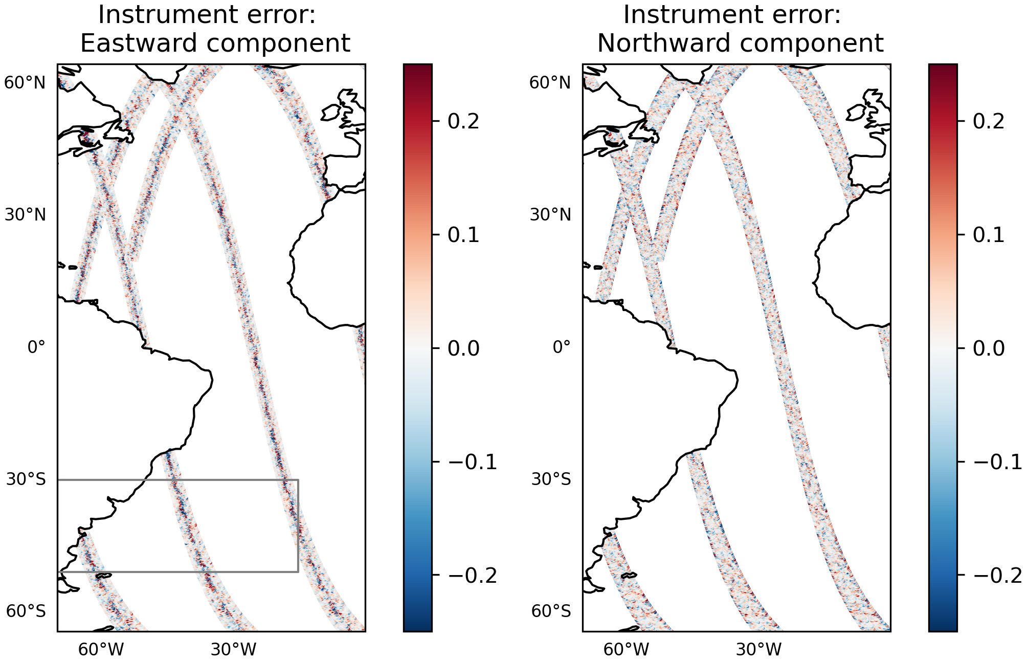
Figure 1 The along swath instrument error (m/s) of the synthetic SKIM TSCVs in the Eastward (left) and Northward (right) direction for the 22^nd of January 2009 shown for the Atlantic region. The grey box in the left plot indicates the South Atlantic Western Boundary region used to calculate the statistics in Figure 6.

Table 1

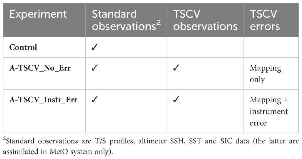
Table 1 Experiment names and the observations assimilated in each one.

A summary of the characteristics of the MetO and MOI forecasting systems used in the A-TSCV OSSEs is given in Table 2. Both the MetO and MOI ocean forecasting systems use the NEMO 3.6 model (Madec et al., 2022) and the OSSEs carried out here were at 1/4° horizontal resolution, with a top model level representative of the upper 1 m of the ocean and were forced with ERA5 atmospheric data. The data assimilation schemes are different. The MetO system uses a multivariate incremental 3DVar-FGAT (first-guess-at-appropriate-time) scheme based on the NEMOVAR code with a one-day time window (Waters et al., 2015). Waters et al. (2024) provide a detailed description of the velocity background error covariances used in the MetO system. The background error covariances are specified by defining a field of background error standard deviations and background error correlation length-scales, where the vertical correlation scales at the surface are dependent on the locally defined mixed layer depth for that day. The MOI system uses a SEEK filter with a fixed basis (the background error covariances are estimated from the mesoscale variability in a historical model run) and has a 7-day time window (Lellouche et al., 2018). A key difference in the two systems is the representation of the multivariate balance in the background error covariances. The multivariate balances are important because they control how information from the velocities is propagated to other model variables. The MetO system uses linearized physical balances to represent the multivariate balance in the background error covariance (Weaver et al., 2005). The balanced relationships are linearized around the daily background model state (meaning they are flow dependent). Water mass conservation is used for temperature-salinity balance, hydrostatic balance is used for SSH balance and geostrophy is used for velocity balance. Meanwhile the MOI system uses multivariate balances derived from the statistics of anomalies from a historical model run. The approach used in the MOI system has the potential benefit of being able to capture multivariate correlations which are not represented by the balanced relationships used in the MetO system, for example ageostrophic velocity balances. However, they have the disadvantage of being climatological estimates and they may include spurious noise if not localized carefully. Idealised experiments where single TSCV innovations are assimilated at locations in the Gulf Stream and Equatorial Atlantic show quite different behaviours in the MetO and MOI system (see Supplementary Figures 1, 2). The vertical propagation of the velocity increments tends to be deeper in the MOI system and in the Equatorial Atlantic the MOI velocity increment reverses sign below 50m depth. The horizontal spread is similar in the Gulf Stream for both systems but we see larger horizontal spread in the Equatorial Atlantic for the MetO system. The magnitude of the velocity increments is larger in the MOI system mainly due to the time window differences. The differences in the structure of the velocity increments reflects differences in the background error covariances used in the two systems. As described in Table 2, the MOI and MetO experiments used different observation thinning for the synthetic SKIM TSCV observations. The MetO system retained one in four of the observations in the along-track and across-track directions (resulting in a 20 km resolution for the thinned data), whereas the MOI system retained one in two in the across-track direction with no thinning in the along-track direction. The MOI system therefore assimilates more of the data (which are at a higher resolution than the model grid).

Table 2

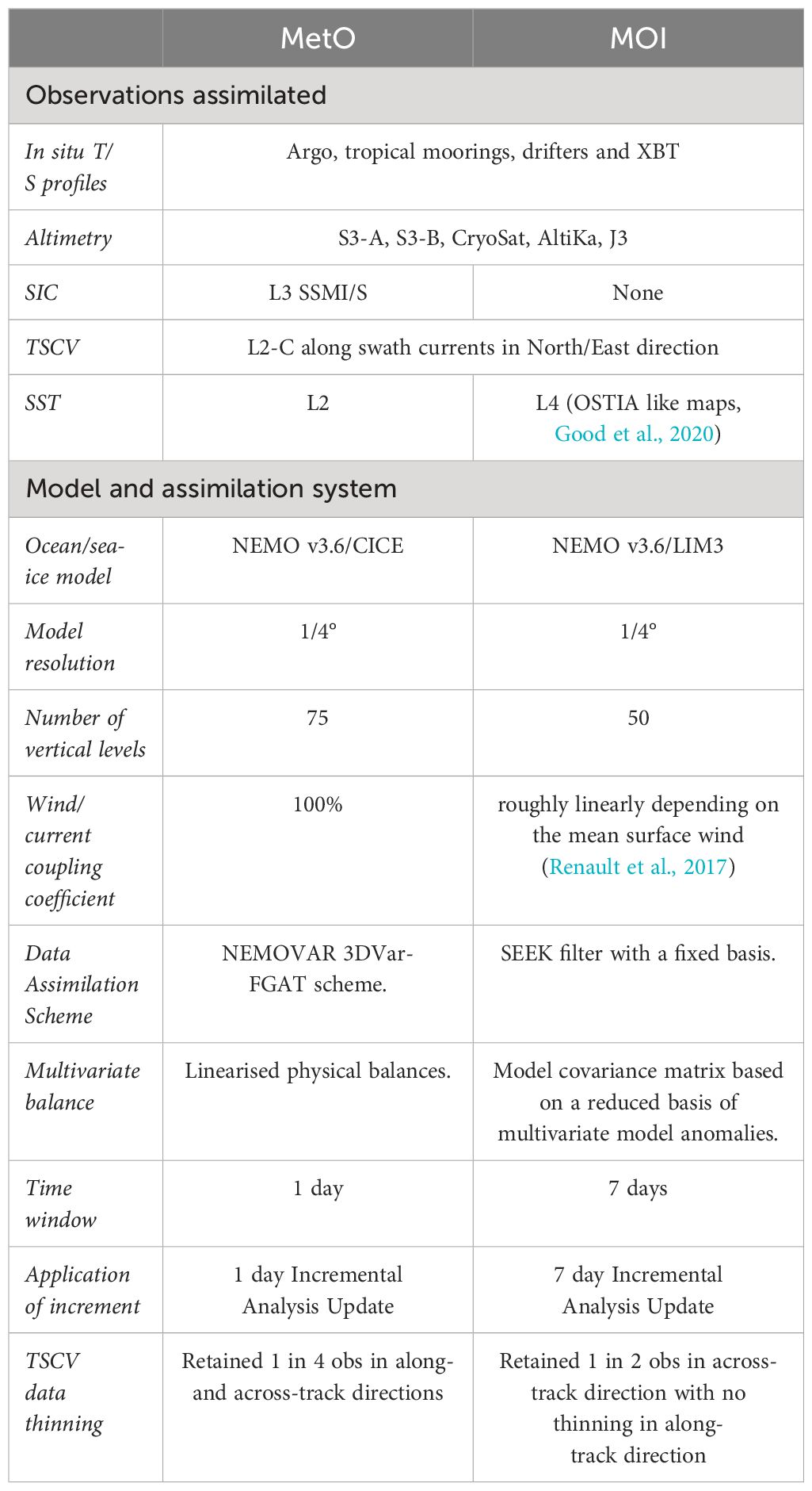
Table 2 Properties of the MetO and MOI forecasting systems use in the A-TSCV OSSEs.

The OSSEs are designed to differ from the NR in order to realistically represent the differences between operational forecasting systems and the true ocean state. These differences are introduced through the different resolution, model version, forcings and initial conditions used in the OSSEs compared to the NR. Table 3 shows some summary global analysis root mean squared error (RMSE) statistics from the MetO and MOI control. These are calculated by taking the daily mean difference of the experiment to the Nature Run, calculating the spatial RMS of the differences, and averaging these throughout the assessment period. The surface and subsurface velocity errors are larger in the MetO control relative to the MOI control. This is partly related to the differences in the model set-up and in particular the wind-current coupling. Using relative winds (equivalent to a wind/current coupling coefficient of 100%) is known to dampen the mean circulation and mesoscale features, while using absolute winds (equivalent to a wind/current coupling coefficient of 0%) over-estimates the mean circulation and mesoscale features (Renault et al., 2020). The MetO system uses relative winds, while the NR uses a 50% wind/current coupling coefficient so it is likely that the MetO system will underestimate current intensity relative to the NR. The MOI system uses the parametrisation proposed by Renault et al. (2017) based on a linearization of the wind/current coupling coefficient which depends on the mean surface wind. This scheme was shown to improve the representation of the ocean - atmosphere energy transfer especially in eddy-rich regions. It is likely to simulate currents and eddies that are more similar to the NR than the MetO system. Differences in the assimilation systems, such as the assimilation time windows and treatment of multivariate balances, are also expected to produce different results in the two control experiments. This impact is seen in all variables, with the MetO control having a lower RMSE for SSH, SST and SSS relative to the MOI control, but larger RMSE for subsurface temperature. It is worth mentioning that the higher SSS RMSE in the MOI system is also partly due to a setting error that strongly decreases the precipitation flux (Mirouze et al., 2024). SST and SSH RMSE are consequently affected through their relationships with SSS. From Barbosa Aguiar et al. (2024) in the standard MetO system global SSH RMSE is 6-7 cm, SST RMSE is ~0.35°C, SSS RMSE is ~0.25 PSU. From Lellouche et al. (2023) the MOI systems global SSH RMSE is 5 cm, SST RMSE is 0.4°C and the salinity at 5 m depth is 0.36 PSU. The global 15m velocity RMSE varies between 13 cm/s and 16 cm/s for MetO and 13 cm/s and 14 cm/s for MOI (Aijaz et al., 2023). These RMSEs are all calculated relative to observations and therefore depend on the sampling of the observation network (unlike the results in Table 3). The impact of sampling is likely to have the largest impact on more sparsely observed quantities such as the currents and salinity, however, the RMSEs in the “real” systems are broadly consistent with the OSSE control errors. This supports the realism of the OSSE experiment design.

Table 3

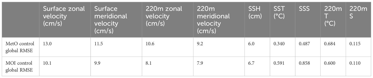
Table 3 Global RMSE statistics for the MetO and MOI control experiments calculated between the 25^th of February and 30^th of December.

3 Results - impact of TSCV assimilation

In this section we assess the impact of the TSCV assimilation in the two systems. Assessment is performed against the NR which is assumed to be the truth in an OSSE framework. Daily mean fields from the OSSEs and NR are used to calculate the statistics presented in this section.

3.1 Impact on surface currents

The impact of assimilating TSCV data with instrument error on the surface velocity RMSE in the two systems is shown in Figure 2. Both systems demonstrate large reductions in RMSE relative to their controls in the equatorial region, with improvements of up to around 20 cm/s in places. The MetO system also has a large reduction in RMSE in the Antarctic Circumpolar Current (ACC) and in the western boundary current regions, e.g. Gulf Stream and Kuroshio. In the MOI system there is a smaller positive impact in those regions. There is not a significant seasonal dependency on these improvements. The MetO system shows some small degradations to zonal surface velocities in the middle of the gyres. A similar degradation is not seen when assimilating the TSCV data without instrument error (Waters et al., 2024). It is likely that the signal to noise ratio of the TSCV observations is low in the center of the gyres when TSCV instrument error is included, particularly in the zonal direction where instrument errors are generally larger. This suggests that the background and observation errors require further tuning in the MetO system to improve the impact of assimilating TSCV observations in the middle of the gyres. An improvement in the global RMSE is retained through 7-day forecasts in both systems, as shown in Figure 3. In the MetO system, the 5-day forecast with TSCV (with instrument error) data assimilated has a lower RMSE than the 1-day forecast from the control experiment without TSCV assimilation, highlighting the major improvement in accuracy of the surface velocities. The reduction in RMSE in the MOI system is not so large but is retained throughout the 7-day forecast. The lower impact in the MOI system is probably due to the fact that the RMS error in the MOI control experiment is already lower than for the MetO control, as discussed in section 2.

Figure 2

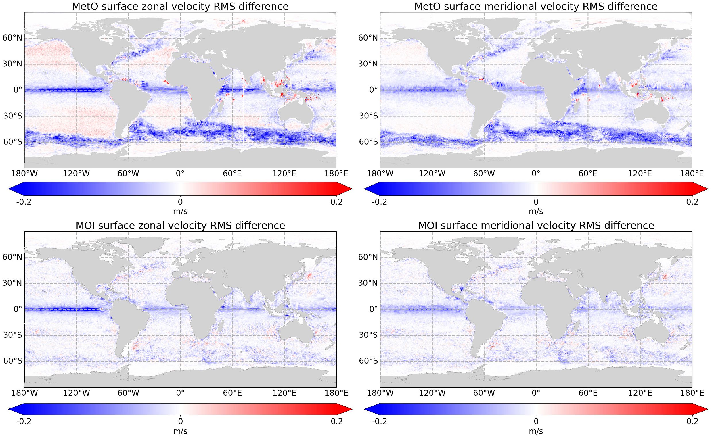
Figure 2 Spatial plot of A-TSCV_Instr_Err RMSE minus control RMSE for surface zonal velocity (left plots) and meridional velocity (right plots), calculated over 25^th February – 30^th December 2009 for the MetO system (top) and MOI system (bottom). Blue areas indicate regions where the A-TSCV experiment has a lower RMSE than the control while red indicates regions where the RMSE is higher.

Figure 3

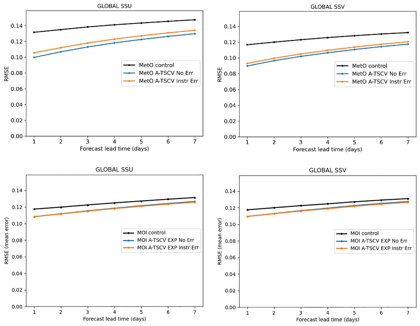
Figure 3 Global forecast RMSE for surface zonal (left) and meridional (right) velocity in m/s for the MetO experiments (top) and MOI experiments (bottom) calculated over 25^th February – 30^th December 2009.

Lagrangian metrics were also used to assess the accuracy of the surface currents. Using the OceanParcels tool (Delandmeter and van Sebille, 2019), particles were seeded globally at ¼ degree resolution and propagated for 6 days from the 9^th of September using the model analysis surface velocities. Figure 4 shows that after 6-days of drifting, the position of objects would be estimated within 50 km of the NR position 74/73% of the time for the MetO/MOI systems respectively, as opposed to 65/67% of the time without the TSCV assimilation. From Figure 4 there is a 1.5 day gain in prediction accuracy when TSCV data are assimilated in both the MetO and MOI systems. The results demonstrate that the drift of objects in the ocean would be forecast much more accurately when assimilating TSCV data than without it.

Figure 4

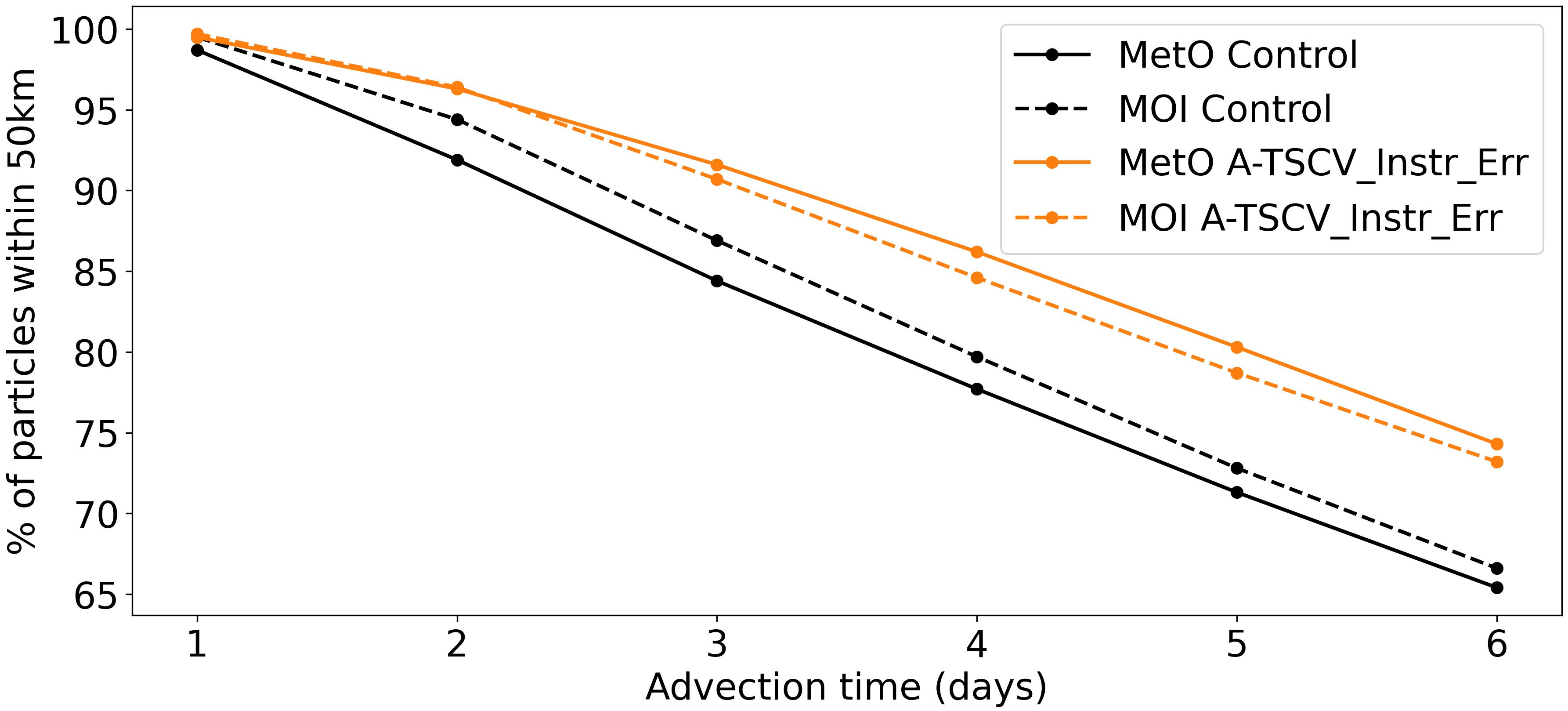
Figure 4 Percentage of particles within 50km of the NR particles as a function of advection time. Black is the control and orange is the A-TSCV Inst Err experiment for MetO (solid line) and MOI (dashed line).

Waters et al. (2024) demonstrated that the unbalanced (ageostrophic) velocity corrections are not well retained in the MetO system. They suggest that away from the equator and coast, Near Inertial Oscillations (NIOs) dominate the ageostrophic velocities and therefore the ageostrophic increments are largely associated with errors in the NIOs. From Waters et al. (2024), when the ageostrophic increments are applied to the model the model tries to respond by rotating the velocities at the NIO frequency, but the 24 hour Incremental Analysis Update method (IAU; Bloom et al., 1996) used to nudge the increments in to the model causes a cancelling affect which dampens the model’s response. When the NIOs are spurious this dampening effect is useful (Raja et al., 2024), but it restricts our ability to correct NIOs when we have valuable information. Waters et al. (2024) proposed a modified version of the IAU, the rotated IAU, which initialises NIOs in the model with the phase and magnitude of the ageostrophic velocity increments. In some short experiments, this method was shown to improve the sub-daily surface velocity RMSE in the Southern-Hemisphere, although results in the Northern-Hemisphere were more mixed. This type of approach could help to further improve the surface currents when TSCV data are assimilated. All the results presented in this paper are using a standard 24 hour IAU in the MetO system and 7 day IAU in the MOI system which means that any corrections to the NIOs are likely to be dampened during the nudging of the increments. The interaction between IAU window and NIOs is also demonstrated in Raja et al. (2024) where they showed an IAU window of 24 hours (or longer) suppress spurious NIOs.

3.2 Impact on subsurface currents

The impact of TSCV assimilation on global sub-surface zonal velocity RMSEs in the MetO and MOI systems is demonstrated through the improvement relative to the MetO and MOI controls, and is shown in Figure 5. The meridional velocity RMSE improvements (not shown) are very similar to the zonal velocity RMSE results. In the MetO system the velocity RMSEs are reduced by 20-30% near the surface with a 10-15% reduction in the MOI system. Again, the lower impact on the MOI system is probably due to the lower RMSE in the MOI control compared to the MetO control. The RMSEs in the MetO system are also improved down to at least 1500 m depth with a reduction of between 7-12% at 1500 m. In the MOI system there are improvements down to about 400 – 500 m depth in the experiment which did not include the instrument errors in the TSCV data, and improvements down to about 800 – 1000 m depth in the experiment which did include the instrument errors. The relatively poor performance in the MOI experiment assimilating TSCV data without instrument errors is thought to be due to overfitting of the TSCV observations. The prescribed observation errors are increased in the experiment assimilating TSCV data with instrument error, which reduces the weight given to the TSCV observations in the assimilation. Mirouze et al. (2024) investigated a more vigorous thinning of the TSCV observations to reduce overfitting. They demonstrate that the additional thinning reduces the degradation to velocity RMSE at depth as well as reducing degradations to temperature and salinity. They show that while overfitting the TSCV observations is less of a problem for the near surface velocities (where the observations are valid) it does cause issues for velocities at depth and this in part is due to the deep propagation of velocity increments in the MOI system (described in section 2). Mirouze et al. (2024) note that, unlike the horizontal background error covariances, the vertical background error covariances in the MOI system are not localised which can lead to spurious vertical projection of the increments. The impact of this is exacerbated by the overfitting of TSCV observations at the surface. This result highlights the importance of both the background error covariance specification and appropriate and careful thinning of the TSCV observations.

Figure 5

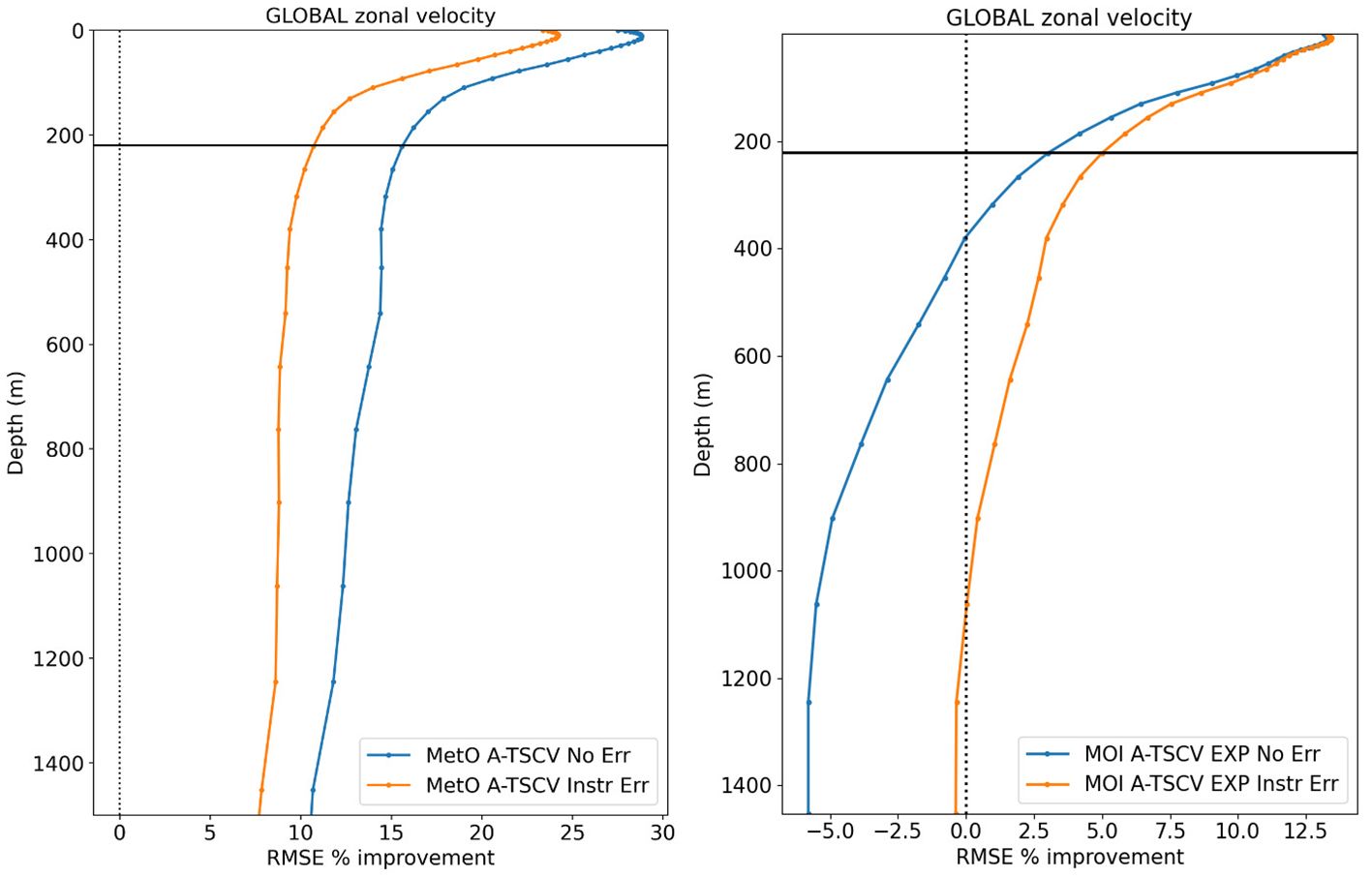
Figure 5 Percentage improvement in global zonal velocity profile RMSEs relative to the control for the MetO experiments (left) and MOI experiments (right) calculated over 25^th February – 30^th December 2009. The horizontal line at 220m indicates the depth of the statistics presented in Table 4.

The depth to which the TSCV data have large impacts varies depending on the region. Two examples are shown in Figure 6 for the equatorial and S. Atlantic western boundary current regions. The zonal velocity impacts are plotted but the meridional velocities show similar impacts. There is around a 40% reduction in RMSE near the surface in both the systems in the equatorial region with the impact reducing to around zero by about 200 – 300 m depth. There is a degradation in RMSE below that depth in the MOI system. In contrast, the two systems show very different impacts in the S.Atlantic western boundary current region. In that region there is a 20 – 30% reduction in RMSE in the MetO system throughout the water column down to 1500 m depth, while the MOI system shows little impact in RMSE near the surface and a degradation in RMSE in the deeper ocean, with worse results in the experiment which did not include the instrument error (attributed to a combination of over-fitting of TSCV observations and the unlimited vertical projection of the corrections by the covariances). The difference in performance in the two systems is due, at least in part, to lower velocity RMS error in the MOI control relative to the MetO control in this region (not show). This is probably related to the difference in the wind/current coupling coefficient, which likely leads to dampened mesoscale features in the MetO system relative to the MOI system and NR. In addition, geostrophy is used to define the velocity balance in the MetO data assimilation scheme so that the part of the TSCV signal due to errors in the geostrophic velocity are projected onto other variables. Waters et al. (2024) showed that TSCV assimilation is able to make significant improvements to the subsurface geostrophic velocities. This produces good improvements to currents in eddy rich regions such as the western boundary currents and ACC.

Figure 6

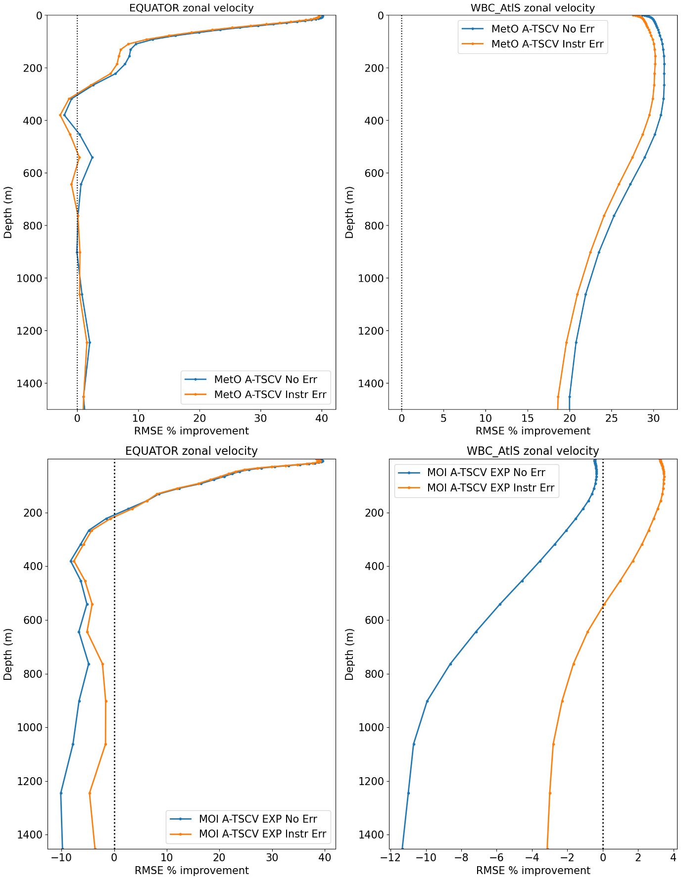
Figure 6 Percentage improvement in regional zonal velocity profile RMSEs relative to the control for the MetO experiments (top) and MOI experiments (bottom) calculated over 25^th February – 30^th December 2009. Left is in the equatorial region (defined as between 3°S and 3°N) and right is in the South Atlantic western boundary current region (defined by the grey box in Figure 1).

3.3 Impact on SSH, temperature and salinity

The MetO and MOI systems show very different impact from the TSCV assimilation on the global SSH RMSEs as shown in Figure 7. In the MetO system there is a 10 – 20% reduction in RMSE from assimilating the TSCV data. The MOI system however shows only a 2 – 4% reduction in RMSE globally, with even smaller improvements when the instrument error is not included.

Figure 7

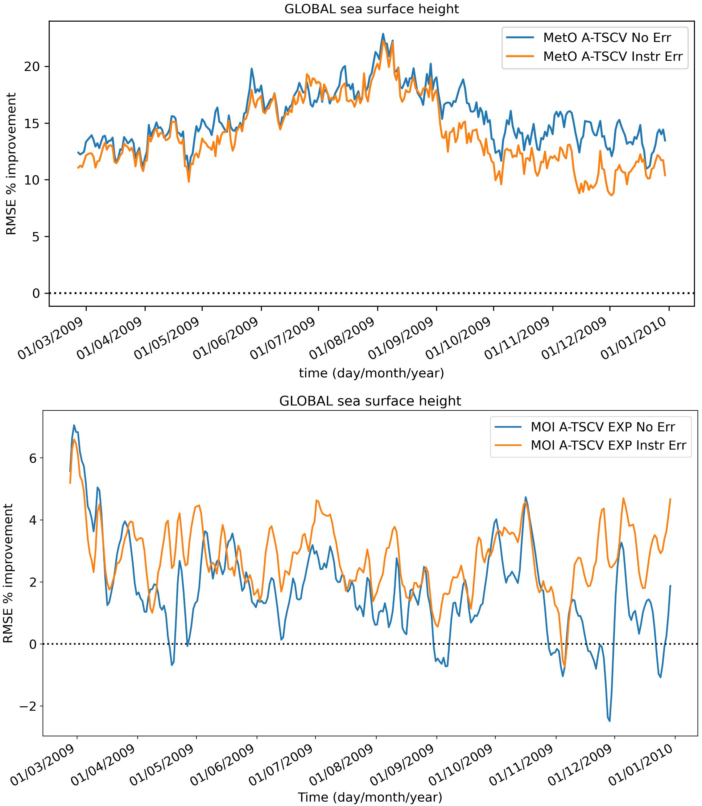
Figure 7 Percentage improvement in Global SSH RMSEs relative to the control for the MetO experiments (top) and MOI experiments (bottom) calculated over 25^th February – 30^th December 2009.

The impact of TSCV assimilation on the temperature and salinity is even more different in the two systems as shown in Figure 8. The MetO system shows a 5 - 10% reduction in global temperature RMSE near the surface. In the experiment which includes the instrument errors, the large surface improvement tails off with depth before increasing again below about 300 m depth, while the experiment which does not include the instrument error maintains a large reduction in RMSE at all depths down to 1500 m. In contrast, the MOI system shows degraded temperature results at all depths with between about 5 and 15% degradation in RMSE at most depths.

Figure 8

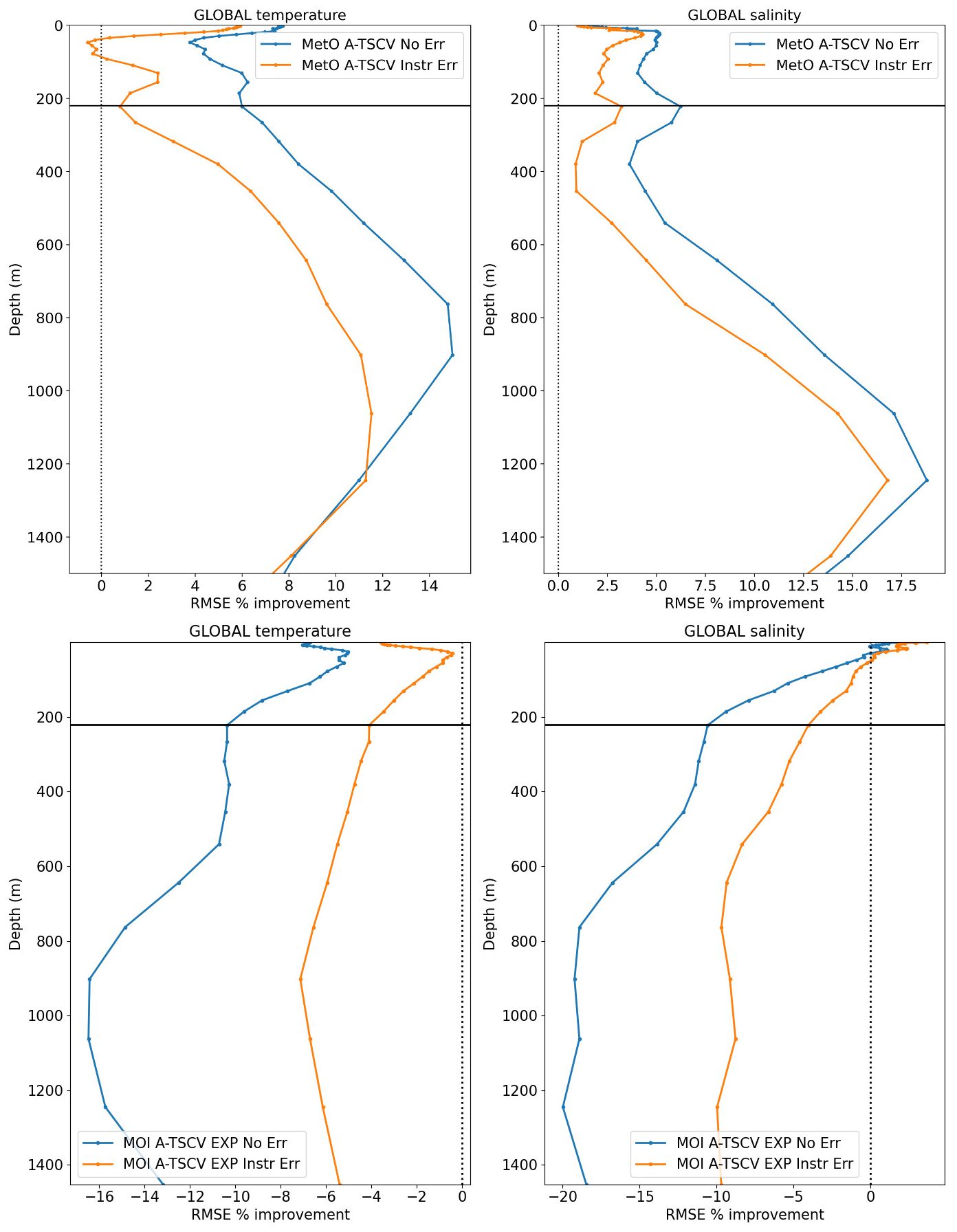
Figure 8 Percentage improvement in Global profile RMSEs relative to the control for the MetO experiments (top) and MOI experiments (bottom) calculated over 25^th February – 30^th December 2009. Left is the temperature RMSE and right is the salinity RMSE. The horizontal line at 220m indicates the depth of the statistics presented in Table 4.

The MetO system shows improvements in global salinity RMSE at all depths with about 5% improvement in the upper 500 m, and even larger reductions in RMSE below that, similar to the improvements seen in temperature. The MOI system has a small improvement in salinity RMSE at the surface, but below the top 50 m there is a degradation in salinity RMSE in the MOI system when assimilating TSCV data.

As mentioned above, an error setting in the MOI system damped down drastically the precipitation flux, yielding a high RMSE for SSS and consequently SST and SSH. The increments for temperature, salinity and SSH, emphasized by the velocity corrections are possibly in conflict with the atmosphere forcings, leading to a RMSE degradation. Differences in results for the two systems may also be related to the different representations of the multivariate balances in the two assimilation schemes. In the MetO system the TSCV assimilation produces significant improvements through geostrophic corrections. The construction of the MOI background error covariances means that the multivariate balance in this system could be less constrained by geostrophy. In fact, Figure 14 in Mirouze et al. (2024) shows that TSCV assimilation improves the prediction of SSH near the equator in the Tropical Atlantic which suggests the MOI background covariances allow TSCV assimilation to make some ageostrophic corrections. Additionally, Mirouze et al. (2024) discussed the impact of potential spurious vertical correlations in the MOI background error covariances as well as the impact of using error covariances estimated from a long historical run which are unable to represent any flow dependence in the system.

3.4 Summary of TSCV assimilation impact

The overall impact of the assimilation of TSCV data on the accuracy of the MetO and MOI operational ocean forecasting systems is significant. A summary of the overall impact of the TSCV assimilation on the model analysis is given in Table 4. This provides the percentage changes in RMSE from assimilating the TSCV data with and without the instrumental error on the MetO and MOI model fields compared to their control run. The analysis RMSE values are also given to provide context to the percentage improvements and to allow direct comparisons to the results in Table 3. Table 5 provides the summary percentage change for the 7-day forecasts and Lagrangian drift assessment.

Table 4

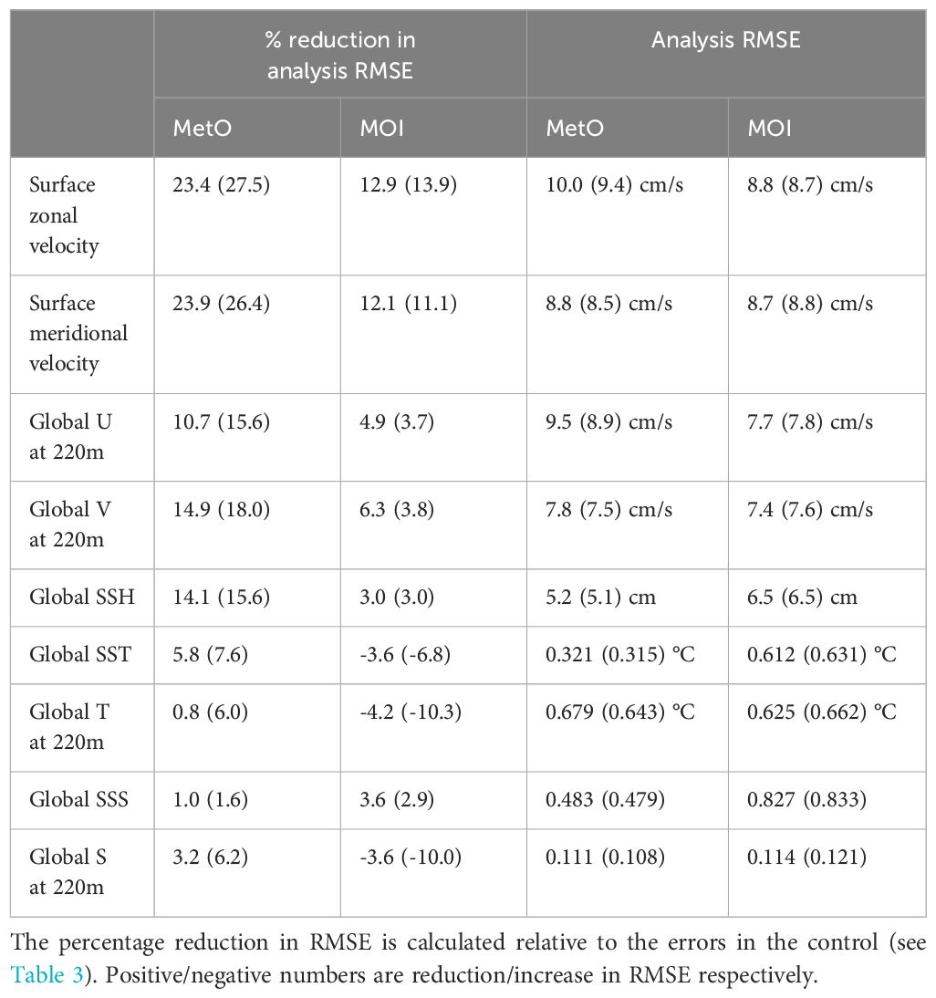
Table 4 Summary table of global analysis RMSE and percentage reduction in analysis RMSE for the A-TSCV_instr_Err (A-TSCV_No_Err) experiments.

Table 5

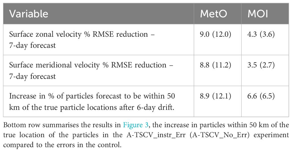
Table 5 First two rows show percentage reduction in Global surface 7 day forecast RMSE for A-TSCV_instr_Err (A-TSCV_No_Err) experiments relative to the control.

We focus on results from the experiment which included the instrumental error since this is the more realistic experiment. As might be expected, the largest impact is on the surface velocity analyses where RMSEs are reduced by up to 24%/13% in the MetO/MOI systems respectively averaged over the global ocean. These impacts carry into the forecasts with a 9%/7% reduction in RMSE at 7-day forecast lead time in the MetO/MOI systems. The percentage of particles forecast to be within 50 km of the true particle locations after drifting for 6 days has increased by 9%/7% in the two systems, a significant improvement for applications which aim to predict the location of particles in the water such as search and rescue, and oil spill modelling. There are also subsurface improvements with 220m analysis velocities improved by up to 15%/6% in the MetO/MOI systems respectively. Improvements to velocity at depth could be useful for improving safety in marine engineering operations and for providing accurate predictions of major ocean currents.

Most of the other variables are impacted much more in the MetO system than the MOI system. The impact on SSH in the MOI system is small with about 3% reduction in global RMSE while the temperature and salinities are overall degraded in the MOI system (although surface salinity is improved slightly). In the MetO system there is a large impact on SSH with 14% reduction in RMSE. Temperature and salinity RMSE are also reduced in the MetO system with 6%/1% reduction in RMSE for SST and sea surface salinity respectively, and substantial reduction in RMSE in the sub-surface too.

4 Requirements for satellite TSCV observations for global ocean prediction systems

In this section we provide a set of requirements for satellite TSCV observations for use with global ocean prediction systems. These are summarized in Table 6 and are based on recommendations and results from literature, input from the international community obtained at a workshop, the authors’ experiences of running operational ocean forecasting systems and the results provided from the ESA A-TSCV OSSEs.

Table 6

Table 6 Requirement for satellite TSCV observations for use in global ocean prediction systems.

A sampling strategy which provides observations for at least 80% of the global ocean in less than 4 to 5 days is recommended, this is equivalent to a temporal resolution of 4-5 days for most of the ocean. The MetO forced global ocean system uses a 1-day data assimilation window (see Table 2) while the Met Office’s coupled global ocean-atmosphere system uses an even shorter assimilation window of 6 hours (Lea et al., 2015). Systems with daily or sub-daily time windows are likely to benefit from observations with high temporal resolution. Wang et al. (2023) showed that the NIOs can be recovered from satellite TSCVs using a wide swath of at least 1800km which allows temporal sampling of less than 12 hours in the midlatitude. Improved data assimilation techniques would be required to make effective use of this high temporal information. Overall, the results from our OSSEs have demonstrated that the impact of TSCV assimilation is well retained in the forecasts. This means that longer observation revisiting time, of the order of days, can provide valuable improvements to our systems.

The recommended horizontal resolution of the satellite TSCV observations is 20 to 50 km to allow mesoscale processes to be resolved over much of the globe. The lower scale is consistent with the baseline horizontal resolution recommended for observing of the surface Ekman and geostrophic currents provided in the 2022 Global Climate Observing System essential climate variable recommendation document (GCOS, 2022).

A measurement accuracy of 10 cm/s in the along and across track direction is recommended for the TSCV observations. Villas Bôas et al. (2019) suggested that surface currents with 10 cm/s accuracy at 30 km spatial resolution and 10 day temporal resolution would significantly improve air-sea flux residuals and surface transport pathway prediction. Our recommendations are slightly more stringent, we recommend this accuracy at higher spatial/temporal resolutions. These are baseline requirements based on today’s accuracy of ocean prediction systems for the scales proposed. From our OSSE controls the accuracy of predicted surface currents varies between 10 and 13 cm/s (see Table 3) while Aijaz et al. (2023) showed that operational ocean forecasting systems produce global daily mean near surface (15 m) currents with an accuracy of 13 -16 cm/s when verified against drifter observation. The authors also showed that the veering angle between the model and observations is mainly within +/-15°. A 10 cm/s accuracy should ensure that TSCV observations provide valuable information when assimilated into global ocean prediction systems. The measurement accuracy is associated with a daily mean estimate, but it can also be refined regionally with larger errors associated with stronger current intensity, as found in western boundary currents and in the ACC. For comparison, the upcoming Harmony mission (Harmony, 2023) has a target accuracy of 25 cm/s at 10 km spatial resolution.

Any satellite TSCV observations should be provided within one day of measurement time in order for them to be used effectively in operational global ocean and coupled forecasting systems.

We recommend that satellite TSCV data is provided at L2b and L2c level (see Table 6 for definitions). The OSSEs performed in this study assimilated L2c TSCV data. This simplified the observation operators used in the MetO and MOI systems, but it also introduces the additional mapping error association with transforming radial velocity to North/East currents. This error is relatively small (~3 cm/s) but it does include some spatial correlations. It may be better to assimilate the lower-level L2b product, which is closer to the “raw” observations, and subsequently have less processing and less complex error characteristics compared to the L2c products. Finally, it is recommended that observation uncertainty estimates are provided with the TSCV data to allow us to accurately represent realistic observation errors within our data assimilation schemes.

5 Conclusion

The expected benefits to operational ocean forecasting of observing TSCV data from space are:

1. Improved accuracy of surface current forecasts through their assimilation, and associated improvements to the currents at depth and other model variables.

2. Improved representation of surface currents through ocean model improvements based on model-observation comparisons.

3. Improved coupled models through better representation of momentum exchanges between ocean, waves, sea-ice and atmosphere.

In the ESA A-TSCV project we have used OSSEs to assess the first of these benefits. In this paper we have summarised the results from the OSSEs performed using the MetO and MOI systems. We have shown that there is the potential to significantly improve global surface currents with TSCV assimilation. This should help to better meet the requirements of users of operational ocean forecasts, for example, search and rescue, oil spill modelling, ship navigation, offshore industry operations and better ocean, waves and sea-ice forecasts in coupled numerical weather prediction (NWP) and seasonal forecasting. In addition, we have seen improvements to the global subsurface currents down to at least 1500 m in the MetO system and 400 m in the MOI system. In the MetO system we also saw substantial improvements to global SSH, temperature and salinity prediction through TSCV assimilation.

It should be highlighted that the impacts summarised above are from idealised experiments. The 1/12^th degree NR used to simulate the observations does not contain all the processes represented by real TSCVs. Tides, Stokes drift and sub-mesoscale processes are not represented in the NR. In addition, we have attempted to represent some of the main sources of error in the model, surface forcing and observations, but it is difficult to represent all of the sources of errors in the real operational systems. The observations of TSCV from real satellite missions would be expected to have larger errors with more complex error characteristics than those used in these experiments. We have not included errors here which have significant spatial correlations since the data assimilation systems cannot currently deal properly with these types of errors, though work is underway to implement methods to represent such errors (e.g. Guillet et al., 2019).

There are some areas where improvements to the assimilation of velocity data could lead to more significant and consistent improvements in the accuracy of the operational forecasting systems if TSCV data were available. Improvements to the velocities in the MetO system away from the equator are predominantly due to corrections to the geostrophic velocities. Some preliminary work on initialising inertial oscillations has taken place (Waters et al., 2024) and further work on this could lead to improved forecasts of these high frequency ageostrophic processes. Additionally, regions such as the middle of the gyres (where we see some degradations to zonal velocity in the MetO system) could be improved by further tuning of the background and observation error covariances. Improvements in the way information from velocity is propagated to other model variables could also lead to further reductions in errors, particularly in the MOI system which saw some degradations in sub-surface temperature, salinity and velocities, even though the surface velocities were improved. The use of different control variables in the assimilation system for velocities could also lead to better control of the divergence and rotational properties of the resulting analyses which could be beneficial in terms of the impact of TSCV assimilation on vertical motions.

Finally, we have outlined a set of requirements for satellite TSCV data for use in global ocean prediction systems which should be considered in the development of future satellite missions.

Data availability statement

The datasets presented in this article are not readily available because the data volumes prevent them being made easily available. Requests to access the datasets should be directed to amVubmlmZXIud2F0ZXJzQG1ldG9mZmljZS5nb3YudWs= and ZXJlbXlAbWVyY2F0b3Itb2NlYW4uZnI=.

Author contributions

JW: Methodology, Validation, Writing – original draft. MM: Conceptualization, Project administration, Writing – original draft. IM: Methodology, Validation, Writing – original draft. ER: Conceptualization, Writing – original draft. RK: Data curation, Writing – review & editing. LG: Data curation, Writing – review & editing. CU: Validation, Visualization, Writing – review & editing. CD: Conceptualization, Writing – review & editing. SG: Validation, Visualization, Writing – review & editing.

Funding

The author(s) declare financial support was received for the research, authorship, and/or publication of this article. The work was funded by the European Space Agency under grant agreement No.4000130863/20/NL/IA.

Conflict of interest

Author LG was employed by the company OceanDataLab.

The remaining authors declare that the research was conducted in the absence of any commercial or financial relationships that could be construed as a potential conflict of interest.

Publisher’s note

All claims expressed in this article are solely those of the authors and do not necessarily represent those of their affiliated organizations, or those of the publisher, the editors and the reviewers. Any product that may be evaluated in this article, or claim that may be made by its manufacturer, is not guaranteed or endorsed by the publisher.

Supplementary material

The Supplementary Material for this article can be found online at: https://www.frontiersin.org/articles/10.3389/fmars.2024.1408495/full#supplementary-material

References

Aijaz S., Brassington G. B., Divakaran P., Régnier C., Drévillon M., Maksymczuk J., et al. (2023). Verification and intercomparison of global ocean Eulerian near-surface currents. Ocean Model. 186, 102241. doi: 10.1016/j.ocemod.2023.102241

CrossRef Full Text | Google Scholar

Ardhuin F., Brandt P., Gaultier L., Donlon C., Battaglia A., Boy F., et al. (2019). SKIM, a candidate satellite mission exploring global ocean currents and waves. Front. Mar. Sci. 6. doi: 10.3389/fmars.2019.00209

CrossRef Full Text | Google Scholar

Barbosa Aguiar A., Bell M. J., Blockley E., Calvert D., Crocker R., Inverarity G., et al. (2024). The Met Office Forecast Ocean Assimilation Model (FOAM) using a 1/12 degree grid for global forecasts. Accepted in Q. J. R. Meteorological Soc.

Google Scholar

Bloom S. C., Takas L. L., Da Silva A. M., Ledvina D. (1996). Data assimilation using incremental analysis updates. Monthly Weather Rev. 124, 1256–1271. doi: 10.1175/1520-0493(1996)124<1256:DAUIAU>2.0.CO;2

CrossRef Full Text | Google Scholar

Davidson F., Alvera-Azcárate A., Barth A., Brassington G. B., Chassignet E. P., Clementi E., et al. (2019). Synergies in operational oceanography: the intrinsic need for sustained ocean observations. Front. Mar. Sci. 6. doi: 10.3389/fmars.2019.00450

PubMed Abstract | CrossRef Full Text | Google Scholar

Delandmeter P., van Sebille E. (2019). The Parcels v2.0 Lagrangian framework: new field interpolation schemes. Geoscientific Model. Dev. 12, 3571–3584. doi: 10.5194/gmd-12-3571-2019

CrossRef Full Text | Google Scholar

Fujii Y., Rémy E., Zuo H., Oke P., Halliwell G., Gasparin F., et al. (2019). Observing system evaluation based on ocean data assimilation and prediction systems: on-going challenges and a future vision for designing and supporting ocean observational networks. Front. Mar. Sci. 6. doi: 10.3389/fmars.2019.00417

PubMed Abstract | CrossRef Full Text | Google Scholar

Gasparin F., Greiner E., Lellouche J.-M., Legalloudec O., Garric G., Drillet Y., et al. (2018). A large-scale view of oceanic variability from 2007 to 2015 in the global high resolution monitoring and forecasting system at mercator oce´an. J. Mar. Syst. 187, 260–276. doi: 10.1016/j.jmarsys.2018.06.015

CrossRef Full Text | Google Scholar

Gasparin F., Guinehut S., Mao C., Mirouze I., Rémy E., King R. R., et al. (2019). Requirements for an integrated in situ atlantic ocean observing system from coordinated observing system simulation experiments. Front. Mar. Sci. 6. doi: 10.3389/fmars.2019.00083

CrossRef Full Text | Google Scholar

Gaultier L., Ubelmann C. (2024). SKIM-like data simulation: System Description, Configuration and Simulations. In preparation for Remote Sensing.

Google Scholar

GCOS. (2022). 2022 GCOS essential climate variable recommendation document. Available at: https://library.wmo.int/viewer/58111/download?file=GCOS-245_2022_GCOS_ECVs_Requirements.pdf&type=pdf&navigator=1.

Google Scholar

Gommenginger C., Chapron B., Hogg A., Buckingham C., Fox-Kemper B., Eriksson L., et al. (2019). A mission to study ocean submesoscale dynamics and small-scale atmosphere-ocean processes in coastal, shelf and polar seas. Front. Mar. Sci. 6. doi: 10.3389/fmars.2019.00457

CrossRef Full Text | Google Scholar

Good S., Fiedler E., Mao C., Martin M. J., Maycock A., Reid R., et al. (2020). The current configuration of the OSTIA system for operational production of foundation sea surface temperature and ice concentration analyses. Remote Sens 12, 720. doi: 10.3390/rs12040720

CrossRef Full Text | Google Scholar

Guillet O., Weaver A. T., Vasseur X., Michel Y., Gratton S., Gurol S. (2019). Modelling spatially correlated observation errors in variational data assimilation using a diffusion operator on an unstructured mesh. Q J. R Meteorol. Soc. 145, 1947–1967. doi: 10.1002/qj.3537

CrossRef Full Text | Google Scholar

Harmony. (2023). Earth explorer 10 mission harmony - mission requirements document. Available at: https://esamultimedia.esa.int/docs/EarthObservation/Harmony_MRD_v1.0_20230616_Issued.pdf.

Google Scholar

Lea D. J., Mirouze I., Martin M. J., King R. R., Hines A., Walters D., et al. (2015). Assessing a new coupled data assimilation system based on the met office coupled atmosphere–land–ocean–sea ice model. Mon. Wea. Rev. 143, 4678–4694. doi: 10.1175/MWR-D-15-0174.1

CrossRef Full Text | Google Scholar

Lellouche J.-M., Greiner E., LeGalloudec O., Garric G., Regnier C., Drévillon M., et al. (2018). Recent updates to the Copernicus marine service global ocean monitoring and forecasting real-time 1/12° high-resolution system. Ocean Sci. 14, 1093–1126. doi: 10.5194/os-14-1093-2018

CrossRef Full Text | Google Scholar

Lellouche J.-M., Le Galloudec O., Regnier C., Van Gennip S., Law Chune S., Levier B., et al. (2023). Quality information document: Global Sea Physical Analysis and Forecasting Product GLOBAL_ANALYSISFORECAST_PHY_001_0240, Copernicus Marine Service (CMS), (1.1). doi: 10.48670/moi-00016

CrossRef Full Text | Google Scholar

Madec G., Bourdallé-Badie R., Chanut J., Clementi E., Coward A., Ethé C., et al. (2022). NEMO ocean engine. doi: 10.5281/zenodo.6334656

PubMed Abstract | CrossRef Full Text | Google Scholar

Martin M. J., Rémy E., Tranchant B., King R. R., Greiner E., Donlon C. (2020). Observation impact statement on satellite sea surface salinity data from two operational global ocean forecasting systems. J. Operat. Oceanogr. 15, 87–103. doi: 10.1080/1755876X.2020.1771815

CrossRef Full Text | Google Scholar

Mirouze I., Rémy E., Lellouche J.-M., Martin M. J., Donlon C. J. (2024). Impact of assimilating satellite surface velocity observations in the Mercator Ocean International analysis and forecasting global 1/4° system. Front. Mar. Sci. 11. doi: 10.3389/fmars.2024.1376999

CrossRef Full Text | Google Scholar

OceanPredict. (2024). Available at: https://oceanpredict.org/.

Google Scholar

Oke P. R., Larnicol G., Fujii Y., Smith G. C., Lea D. J., Guinehut S., et al. (2015a). Assessing the impact of observations on ocean forecasts and reanalyses: part 1, global studies. J. Operat. Oceanogr. 8, s49–s62. doi: 10.1080/1755876X.2015.1022067

CrossRef Full Text | Google Scholar

Oke P. R., Larnicol G., Jones E. M., Kourafalou V., Sperrevik A. K., Carse F., et al. (2015b). Assessing the impact of observations on ocean forecasts and reanalyses: part 2, regional applications. J. Operat. Oceanogr. 8, s63–s79. doi: 10.1080/1755876X.2015.1022080

CrossRef Full Text | Google Scholar

Raja K. J., Buijsman M. C., Bozec A., Helber R. W., Shriver J. F., Wallcraft A., et al. (2024). Spurious internal wave generation during data assimilation in eddy resolving ocean model simulations. Ocean Model. 188, 102340. doi: 10.1016/j.ocemod.2024.102340

CrossRef Full Text | Google Scholar

Renault L., Masson S., Arsouze T., Madec G., McWilliams J. C. (2020). Recipes for how to force oceanic model dynamics. J. Adv. Modeling Earth Syst. 12, e2019MS001715. doi: 10.1029/2019MS001715

CrossRef Full Text | Google Scholar

Renault L., McWilliams J. C., Masson S. (2017). Satellite observations of imprint of oceanic current on wind stress by air-sea coupling. Sci. Rep. 7, 17747. doi: 10.1038/s41598-017-17939-1

PubMed Abstract | CrossRef Full Text | Google Scholar

Rodríguez E., Bourassa M. A., Chelton D., Farrar J. T., Long D. G., Perkovic-Martin D., et al. (2019). The winds and currents mission concept. Front. Mar. Sci. 6. doi: 10.3389/fmars.2019.00438

CrossRef Full Text | Google Scholar

Torres H., Wineteer A., Klein P., Lee T., Wang J., Rodriguez E., et al. (2023). Anticipated capabilities of the ODYSEA wind and current mission concept to estimate wind work at the air–sea interface. Remote Sens. 15, 3337. doi: 10.3390/rs15133337

CrossRef Full Text | Google Scholar

Villas Bôas B., Ardhuin F., Ayet A., Bourassa M. A., Brandt P., Chapron B., et al. (2019). Integrated observations of global surface winds, currents, and waves: requirements and challenges for the next decade. Front. In Mar. Sci. 6. doi: 10.3389/fmars.2019.00425

CrossRef Full Text | Google Scholar

Wang J., Torres H., Klein P., Wineteer A., Zhang H., Menemenlis D., et al. (2023). Increasing the observability of near inertial oscillations by a future ODYSEA satellite mission. Remote Sens 15, 4526. doi: 10.3390/rs15184526

CrossRef Full Text | Google Scholar

Waters J., Lea D. J., Martin M. J., Mirouze I., Weaver A., While J. (2015). Implementing a variational data assimilation system in an operational 1/4 degree global ocean model. Q. J. R. Meteorological Soc. 141, 333–349. doi: 10.1002/qj.2388

CrossRef Full Text | Google Scholar

Waters J., Martin M. J., Bell M. J., King R. R., Gaultier L., Ubelmann C., et al. (2024). Assessing the potential impact of assimilating total surface current velocities in the Met Office’s global ocean forecasting system. Front. Mar. Sci. 11. doi: 10.3389/fmars.2024.1383522

CrossRef Full Text | Google Scholar

Weaver A. T., Deltel C., Machu E., Ricci S., Daget N. (2005). A multivariate balance operator for variational ocean data assimilation. Q. J. R. Meteorol. Soc. 131, 3605–3625. doi: 10.1256/qj.05.119

CrossRef Full Text | Google Scholar