Attribution analysis and forecast of salinity intrusion in the Modaomen estuary of the Pearl River Delta

Under the influence of climate change and human activities, the intensification of salinity intrusion in the Modaomen (MDM) estuary poses a significant threat to the water supply security of the Greater Bay Area of Guangdong, Hong Kong, and Macao. Based on the daily exceedance time data from six stations in the MDM waterway for the years 2016-2020, this study conducted Empirical Orthogonal Function (EOF) and decision tree analyses with runoff, maximum tidal range, and wind. It investigated the variation characteristics and key factors influencing salinity intrusion. Additionally, Long Short-Term Memory (LSTM) networks and Convolutional Neural Networks (CNN) were employed to predict the severity of salinity intrusion. The results indicated that: (1) the first mode (PC1) obtained from EOF decomposition explained 89% of the variation in daily chlorine exceedance time, effectively reflecting the temporal changes in salinity intrusion; (2) the largest contributor to salinity intrusion was runoff (40%), followed by maximum tidal range, wind speed, and wind direction, contributing 25%, 20%, and 15%, respectively. Salinity intrusion lagged behind runoff by 1-day, tidal range by 3 days, and wind by 2 days; North Pacific Index (NPI) has the strongest positive correlation with saltwater intrusion among the 9 atmospheric circulation factors. (3) LSTM achieved the highest accuracy with an R² of 0.89 for a horizon of 1 day. For horizons of 2 days and 3 days, CNN exhibited the highest accuracy with R² values of 0.73 and 0.68, respectively. This study provides theoretical support for basin scheduling and salinity intrusion prediction and serves as a reference for ensuring water supply security in coastal areas.

1 Introduction

Saltwater intrusion is a common natural hydrological phenomenon in coastal estuarine areas. In recent years, climate change and human activities have led to an increasingly severe intrusion of saltwater into estuaries, posing a serious threat to the water supply security of coastal cities and the stability of estuarine ecosystems. Moreover, there is a trend of aggravation in the coming decades (Zhang et al., 2019; Loc et al., 2021; Prayag et al., 2023). In 2021, the eastern region of China’s Pearl River Basin experienced its severest drought since 1961. Saltwater intrusion into the water intake points at the Guangchang (GC) pumping station and the Lianshiwan (LSW) sluice gate in the Zhuhai-Macau water supply system occurred earlier than usual, on June 21st and August 3rd respectively, breaking historical records. Additionally, in 2022, extreme high temperatures across the entire Yangtze River Basin led to severe dry spells during the flood season in the middle and lower reaches, resulting in a high-intensity saltwater intrusion phenomenon observed at the river mouth on August 10th. In the summer of 2022, Europe experienced an extended drought, significantly reducing the discharge of the River Rhine for several months. Consequently, chloride concentrations in the tidal portion of the river rose above 8000 mg/L (Anoek and Hudson, 2022). Furthermore, in the coastal delta regions of India, Bangladesh, and Vietnam, more than 25 million people are at risk of drinking salty water (Shammi et al., 2019; Das et al., 2021). Therefore, it is crucial to study the response relationships between various factors in the evolution of saltwater intrusion and to accurately forecast saltwater intrusion. This is essential for guiding fine-tuned salinity control in estuarine areas and ensuring urban water supply security (Rohmer and Brisset, 2017).

The Pearl River Basin comprises a complex river network system, formed by multiple rivers including the West River, North River, and East River, along with numerous tributaries in the Pearl River Delta region, ultimately connecting to the South China Sea through the Pearl River Estuary. The Pearl River Estuary is the core area of the Guangdong-Hong Kong-Macao Greater Bay Area, where urban water supply primarily relies on river-based sources, constituting 70.4% of the total water supply. However, some areas lack sufficient storage capacity, making them highly susceptible to saltwater intrusion during the dry season. Among the eight major estuary channels, Modaomen (MDM), located at the mouth of the Pearl River, frequently experiences saltwater intrusion disasters, posing a serious threat to the water supply of Macau, Zhuhai, and Zhongshan, and presenting a daunting challenge to the high-quality development of the national economy (Tang et al., 2020; Zhou et al., 2020; Hu et al., 2024). Abundant research has indicated that saltwater intrusion in the MDM estuary has been influenced by various driving forces, including runoff, tides, wind, and mean sea level (Gong and Shen, 2011; Chen, 2015; Lin et al., 2019; Gong et al., 2022). Gong and Shen (2011) pointed out that the upstream intrusion distance of saltwater in the MDM waterway generally exhibits an inverse proportionality to the magnitude of upstream river discharge, following a power-law relationship. Lin et al. (2019) discovered that wind has a significant impact on the saltwater intrusion in the MDM waterway. However, tides and river discharge remain the main driving factors. Moreover, due to the generally unstable nature of external driving forces, different factors interact and superimpose across various time scales, exhibiting a certain degree of temporal lag. All of the above factors contribute significantly to the formidable challenge of forecasting estuarine saltwater intrusion.

Currently, saltwater intrusion prediction methods mainly fall into two categories: numerical simulation (Liu et al., 2017; Pappa et al., 2017; Ye et al., 2017) and data-driven approaches (Zhou et al., 2017; Hunter et al., 2018). Numerical simulation models can effectively replicate the physical processes of salt transport. However, these models require substantial computational resources for setup, compilation, configuration, and execution. Additionally, extensive calibration and validation are needed using real-world data on topography, hydrology, tidal flows, salinity, etc (Lathashri and Mahesha, 2015; Zhang et al., 2015). In situations where reliable forecasts are needed but there is insufficient data on influential factors, data-driven models have clear advantages. These models uncover nonlinear relationships between input factors and output targets (Hu et al., 2019). Data-driven models can generally be categorized into traditional statistical models and the more recently emerged machine learning models. For instance, Qiu and Wan (2013) successfully utilized statistical models to predict salinity in the Caloosahatchee River Estuary. However, saltwater intrusion processes are influenced by various factors such as river flow, tidal currents, wind, precipitation, terrain, and human activities, exhibiting high complexity and nonlinearity among variables. The ability of traditional statistical models to capture the nonlinear characteristics of hydrological processes is limited (Yaseen et al., 2015; Tian, 2019). Machine learning models possess strong nonlinear learning capabilities and high computational efficiency. For example, Liu et al. (2021) employed the Bayesian Model Averaging (BMA) method to integrate predictions from Random Forest (RF), Support Vector Machine (SVM), and Elman Neural Network (ENN) models to forecast monthly-scale saltwater intrusion in the Pearl River Delta. Hoai et al. (2022) applied multiple machine learning algorithms including Multiple Linear Regression (MLR), Random Forest Regression (RFR), and Artificial Neural Network (ANN) to predict saltwater intrusion in the Mekong Delta, with results indicating that the ANN algorithm exhibited better predictive performance.

Although neural networks offer strong nonlinear learning abilities with high accuracy, but they may face challenges like local minimum convergence and overfitting. SVM require careful kernel function selection, influencing predictive accuracy (Xiao et al., 2014; Gao and Su, 2020; Ren, 2021; Zhang et al., 2022). With the continuous improvement in data availability and computing power in recent years, deep learning has become a crucial component of time series prediction models. However, selecting the most suitable deep neural network and its parameters is a complex task that demands substantial expertise. Lara–Benítez et al. (2021) conducted an extensive study on deep neural network time series prediction. The results suggested that LSTM and CNN were the optimal predictive models. LSTM demonstrated the highest accuracy, while CNN exhibited both stability and efficiency across various parameter configurations. Numerous studies have demonstrated that LSTM and CNN models are capable of capturing long-term correlations in time series data, providing excellent representation of spatiotemporal features in hydrological, meteorological, and geographical datasets. Particularly, they have exhibited strong performance in precipitation, runoff, and flood forecasting (Kratzert et al., 2018; Le et al., 2019; Barzegar et al., 2020; Kao et al., 2020; Tian et al., 2023). For instance, Wullems et al. (2023) utilized water level, discharge and wind speed as inputs and employed LSTM model to achieve reasonable predictions of chloride concentration at individual stations in the Rhine-Meuse Delta in the Netherlands for up to 7 days.

Current research on saltwater intrusion in estuaries often focuses on individual monitoring stations. However, estuarine areas typically have multiple monitoring stations, and the daily variations in chloride concentration at each station can be significant. Relying solely on data from a single station may not accurately represent the overall variation in saltwater intrusion across the estuary, making it difficult to quantify the severity of the intrusion. Based on the statistical analysis of the temporal trends in daily chlorine content exceeding standards at six stations from 2016 to 2020 in the MDM waterway, this study selects influencing factors such as runoff, tidal level, and wind. The primary focus is on the following tasks: (1) interpolating missing chloride concentration data; (2) using Empirical Orthogonal Function (EOF) analysis to understand spatiotemporal patterns in daily exceedance times and their relationships with influencing factors; (3) quantifying contributions and temporal characteristics of factors using decision tree analysis; (4) employing the cross-wavelet method to analyze the primary driving forces of saltwater intrusion by selecting the factors with the greatest contribution; and (5) predicting saltwater intrusion severity with LSTM and CNN methods. The goal is to identify key factors influencing saltwater intrusion, enhance simulation and prediction techniques, and contribute insights for ensuring water supply security in coastal areas.

2 Study area and data

The Pearl River Basin has the second-highest annual runoff in China, following the Yangtze River. However, the distribution of runoff is uneven, with the dry season accounting for only 23% of the total. This makes the region highly vulnerable to saltwater intrusion during the dry season. MDM, one of the eight estuaries in the Pearl River estuary (Figure 1), is located downstream in the Xijiang River Basin. It plays a crucial role as the primary channel for flood discharge and sediment transport in the Xijiang River, contributing around 27% of the total runoff into the Pearl River estuary. Since the 21st century, saltwater intrusion in the MDM waterway has exhibited new characteristics. These include earlier onset, prolonged duration, and increased upstream intrusion distance. Severe instances of saltwater intrusion occurred during the dry seasons of 2004-2005, 2005-2006, 2009-2010, 2011-2012, and 2020-2023. For example, during the 2019-2020 dry season, Zhongshan City faced 10 instances of saltwater intrusion, affecting 46% of its water supply capacity. In 2021, saltwater intrusion at the GC pumping station and LSW sluice gate occurred earlier than usual, on June 21st and August 3rd, respectively, breaking records. Subsequently, in 2022, the Pearl River estuary experienced 11 severe saltwater intrusion events, causing all intake points along the MDM waterway to exceed chlorine standards from December 4th onwards. Notably, the Pinggang pumping station saw chlorine levels exceed standards for 10 consecutive days, disrupting water supply in Zhuhai for approximately two weeks.

Figure 1

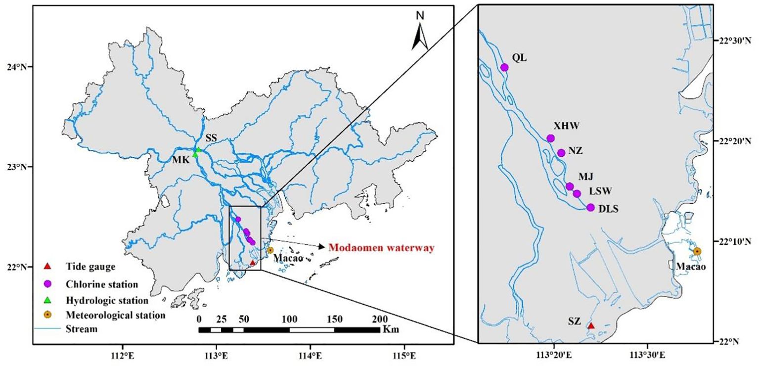
Figure 1 Study area and site distribution.

In this study, hourly chloride concentration data from 2016 to 2020 during the dry season were collected from six automated monitoring stations (Denglongshan (DLS), LSW, Majiao (MJ), Nanzhen (NZ), Xihewai (XHW), Quanlu (QL)) in the MDM waterway, sourced from the Zhongshan Water Affairs Bureau’s official website. As these stations are typically situated close to the shore, the chloride data primarily represent surface water salinity. Data for the annual period from October 1st to March 31st of the following year were considered. Hourly runoff data from Makou (MK) and Sanshui (SS) stations during the period, along with that from Wuzhou (WZ) station between 1961 and 2020, were sourced from the Hydrological Yearbook and the National Water and Rainfall Information Network of the Ministry of Water Resources. Tidal data for Sanzao (SZ) were sourced from the Hydrological Yearbook, and wind speed and direction data for the Macao station were obtained from the China Meteorological Data Network.

The teleconnection data were obtained from the Hadley Observing Centre of the UK Met Office, covering monthly records from 1961 to 2020. Nine major climate teleconnection indices were selected, including the El Niño-Southern Oscillation Index (ENSO), Atlantic Multidecadal Oscillation Index (AMO), North Atlantic Oscillation Index (NAO), Arctic Oscillation Index (AO), Pacific Decadal Oscillation Index (PDO), Indian Ocean Dipole Index (DMI), North Pacific Index (NPI), Pacific-North American Oscillation Index (PNA), and Sunspot Index (SSI).

3 Methodology

3.1 Imputation methods for missing data

Due to various objective and subjective factors, some time series data were missing in the chlorine content data from automatic monitoring stations. Various data imputation techniques are widely used across research domains, including specific value replacements (such as mean, mode, or median), multivariate imputation, K-nearest neighbors (KNN), and the expectation maximization (EM) algorithm. This study evaluated three imputation methods—median, KNN, and multiple imputation—based on complete datasets. Through data imputation, a comprehensive and rich dataset was constructed, providing a solid sample basis and data support for subsequent in-depth data analysis and exploration work, thus ensuring the scientificity and accuracy of research conclusions.

3.1.1 Median

Median imputation, a commonly used method for filling missing values, estimates the average or most common value for a given attribute based on observed data. However, it is known to have limitations, including the potential for significant computational errors (Hadeed et al., 2020; Dahj and Ogudo, 2023).

3.1.2 KNN

The KNN algorithm exhibits strong robustness when filling in missing data in complex datasets (Habib et al., 2023). It relies on the positions of the K nearest known data points in the feature space to impute missing values, determining classification based on proximity. However, a low number of neighbors may be influenced by outliers, while a high number may suffer from irrelevant data interference (Zhang et al., 2017; Sahoo and Ghose, 2022). This method is most effective for imputing missing values in observations with overlapping intersections.

3.1.3 Multiple imputation

MICE (Multivariate Imputation by Chained Equations) is a method for handling missing values through repeated simulations. It generates a complete dataset from an incomplete one by imputing missing data using the Markov Chain Monte Carlo (MCMC) method in each simulated dataset (Wijesuriya et al., 2020; Beesley et al., 2021). The imputation process involves three steps: initially, missing data in the original dataset are imputed using the MCMC method. Then, statistical models analyze and evaluate the completed data. Finally, the imputed complete dataset is generated as output.

3.2 EOF decomposition

Since the MDM waterway comprises six monitoring stations, the exceedance time variation differs significantly among them. Utilizing data from a single station cannot capture the overall fluctuation of saltwater intrusion across the estuary. Hence, this study conducted EOF analysis on the daily exceedance time data from all six stations for the period 2016-2020. EOF analysis is a method for examining structural features and extracting principal characteristics from matrix data. The basic principle involves decomposing the matrix representing daily exceedance durations across m monitoring stations over time (Björnsson and Venegas, 1997; Karunarathna et al., 2012; Lin et al., 2019). Mathematically, we can view this field as an m-dimensional vector X, where X represents n samples X₁, X₂, …, X_n, each sample being an m-dimensional column vector denoted as X_n (t=1,2,…,n). Assuming each station has daily exceedance time data for n time points, the daily exceedance duration (x_ij)_mn at any station i and time point j can be expressed as a linear combination of m spatial functions eof_ikand m temporal functions pc_kj(k=1,2,…,m). As illustrated in the following formula:

$\begin{array}{ll}{x}_{ij}={\displaystyle \sum _k^{m}eo{f}_{ik}}p{c}_{kj}=eo{f}_{i1}p{c}_{1j}+eo{f}_{i2}p{c}_{2j}+\cdots +eo{f}_{im}p{c}_{mj}& (1)\end{array}$

The matrix form is shown in Equation (2):

$\begin{array}{ll}X=EOF·PC=\left[\begin{array}{cccc}eo{f}_{11}& eo{f}_{12}& \cdots & eo{f}_{1m}\\ eo{f}_{21}& eo{f}_{22}& \cdots & eo{f}_{2m}\\ ⋮& ⋮& \ddots & ⋮\\ eo{f}_{m1}& eo{f}_{m2}& \cdots & eo{f}_{mm}\end{array}\right]·\left[\begin{array}{cccc}p{c}_{11}& p{c}_{12}& \cdots & p{c}_{1n}\\ p{c}_{21}& p{c}_{22}& \cdots & p{c}_{2n}\\ ⋮& ⋮& \ddots & ⋮\\ p{c}_{m1}& p{c}_{m2}& \cdots & p{c}_{mn}\end{array}\right]& (2)\end{array}$

Where X is the matrix of $m\times n$ order, which indicates the daily exceeding time of m stations at n moments, $x_{ij}(i=1,2,\cdots ,m;j=1,2,\cdots ,n)$ indicates the daily exceeding time of i station at j moment, and the decomposed EOF and PC are dimensionless.

The column vectors of EOF represent spatial feature vectors corresponding to each eigenvalue, while each row of PC represents the temporal coefficients for each mode. The decomposition ensures orthogonality with other functions, with the functions arranged based on the eigenvalues of the covariance matrix.

The specific steps are as follows:

Multiplying the right side of Equation (1) by the transpose of the daily exceedance time series matrix X, denoted as $X^{\prime }$, we obtain:

$\begin{array}{ll}X{X}^{\prime }=EOF·PC·P{C}^{\prime }·EO{F}^{\prime }& (3)\end{array}$

Decomposing this real symmetric matrix, we obtain:

$\begin{array}{ll}X{X}^{\prime }=EOF·\Lambda ·EO{F}^{\prime }& (4)\end{array}$

Where, $\Lambda$ represents the diagonal matrix composed of the eigenvalues of matrix $X{X}^{\prime }$, and EOF is the matrix composed of the column vectors of its corresponding eigenvectors.

Therefore, Equations (3) and (4) lead to the following:

$\begin{array}{ll}PC·P{C}^{\prime }=\Lambda & (5)\end{array}$

The eigenvectors have the following properties:

$\begin{array}{ll}P{C}^{\prime }·PC=PC·P{C}^{\prime }=I& (6)\end{array}$

Equations (5) and (6) clearly exhibit orthogonality. Therefore, it can be inferred that the spatial function matrix EOF can be obtained from the eigenvectors of matrix $X{X}^{\prime }$, while the temporal function matrix PC can be obtained by left-multiplying $EO{F}^{\prime }$ with Equation (1), that is Equation (7):

$\begin{array}{ll}PC=EO{F}^{\prime }·X& (7)\end{array}$

The k-th row element of the temporal function matrix PC can be expressed as Equation (8) :

$\begin{array}{ll}p{c}_{kj}=eo{f}_{1k}{x}_{1j}+eo{f}_{2k}{x}_{2j}+\cdots +eo{f}_{mk}{x}_{mj}& (8)\end{array}$

The product of the first p temporal functions and their corresponding spatial functions (where p< m)) is taken as an estimate of the observed value x_ij at the i-th spatial point and j-th time point in the original matrix of daily chlorine concentration exceeding the threshold. Therefore, the fit can be represented by eigenvalues. When the contribution rate of the first p eigenvalues reaches a substantial value, the corresponding first p temporal functions and their associated spatial functions can roughly reflect the variations in this region.

3.3 Decision tree method

Decision tree analysis is a risk-based decision-making method that compares different scenarios using trees from probability and graph theory to obtain optimal solutions. It is a significant method in data mining, commonly employing classification and regression trees (CART) to intuitively reflect outcomes (Park et al., 2013; Bae, 2019). The feature importance of a decision tree measures each feature’s contribution to the target value, making it useful for feature selection and model interpretation. Being a non-parametric model, it doesn’t require assumptions about samples and can handle complex datasets. The attribute selection methods for decision trees include Information Gain (ID3), Gain Ratio (C4.5), and Gini Index (CART). This study utilized CART to explore the main controlling factors of saltwater intrusion, assessing the importance and contribution of various influencing factors.

3.4 Cross-wavelet transform

The cross-wavelet transform is an advanced tool for time-frequency analysis, revealing the close interaction between two time series. It captures detailed signal characteristics and demonstrates its importance in dynamic property research. Through the cross-wavelet transform, we can discern the correlation between two sequences in different energy regions: the wavelet energy spectrum focuses on high-energy areas, while the wavelet coherence spectrum emphasizes low-energy regions.

Cross-wavelet transform is defined as W^XY=W^XW^Y*, where “*“ denotes complex conjugate. ∣W^XY∣ reflects the cross-wavelet power spectrum, while the argument of arg (W^xy) represents the relative phase between the two time series in the time-frequency domain. The theoretical distributions of cross-wavelet power between the two time series and their background power spectra are as as Equation (9):

$\begin{array}{ll}D(\left|\frac{W_n^X(s)W_n^{Y\ast }(s)}{{\sigma }_X{\sigma }_Y}\right|<p)=\frac{Z_v(p)}{v}\sqrt{P_k^X{P}_k^Y}& (9)\end{array}$

Where, Z_v(p) represents the confidence level of the probability density function constructed using the double-parameter ${\chi }^2$ integrated variance distribution; ${\sigma }_X$ and ${\sigma }_Y$ are the standard deviations of the respective time series data; v is the degree of freedom.

The cross-wavelet energy spectrum unveils phase coupling and common characteristics among different time series, while the wavelet coherence spectrum precisely evaluates the correlation level between time series at a local scale. Its expression is as Equation (10):

$\begin{array}{ll}{R}_n^2(s)=\frac{{\left|S(s^{-1}{W}_n^{XY}(s))\right|}^2}{S(s^{-1}{\left|W_n^X(s)\right|}^2)·S(s^{-1}{\left|W_n^Y(s)\right|}^2)}& (10)\end{array}$

Where, S represents the smoother, defined as $S(W)=S_{\text{scale}}(S_{time}(W_n(s)))$;S_scale denotes the smoothing along the scaling dimension achieved by wavelet transform; S_time refers to the smoothing along the time translation dimension performed by wavelet transform.

3.5 Deep neural network prediction model

3.5.1 LSTM

The LSTM addresses challenges in traditional models during long-time sequence training, overcoming issues such as gradient explosions, vanishing gradients, and difficulties in preserving historical data over extended periods (Hochreiter and Schmidhuber, 1997). LSTM’s self-connected hidden layer captures both cell state and hidden layer state from the previous time step, utilizing ‘forget gates,’ ‘input gates,’ and ‘output gates’ to control information transmission and updating. Specifically, the ‘forget gate’ controls the forgetting of cell state information, the ‘input gate’ manages the input of new information, and the ‘output gate’ regulates the output of cell state information.

The LSTM hidden layer structure, as depicted in Figure 2A, involves C_t-1 and C_t for cell state information at time steps t-1 and t. ${\tilde{C}}_t$ represents the candidate update information at time step t, h_t-1 and h_t denote the hidden layer state information at time steps t-1 and t, X_t is the input value at time step t, $\sigma$ is the sigmoid function, and f_t, i_t, and o_t are the control coefficients for the ‘forget gate’, ‘input gate’, and ‘output gate’, respectively. These coefficients are computed using the Sigmoid function, regulating gate opening and closing. The tanh function computes the new candidate cell state within a range of -1 to 1. By adjusting the control coefficients of the sigmoid gates, it determines which information to retain or update, thereby updating the cell state information.

Figure 2

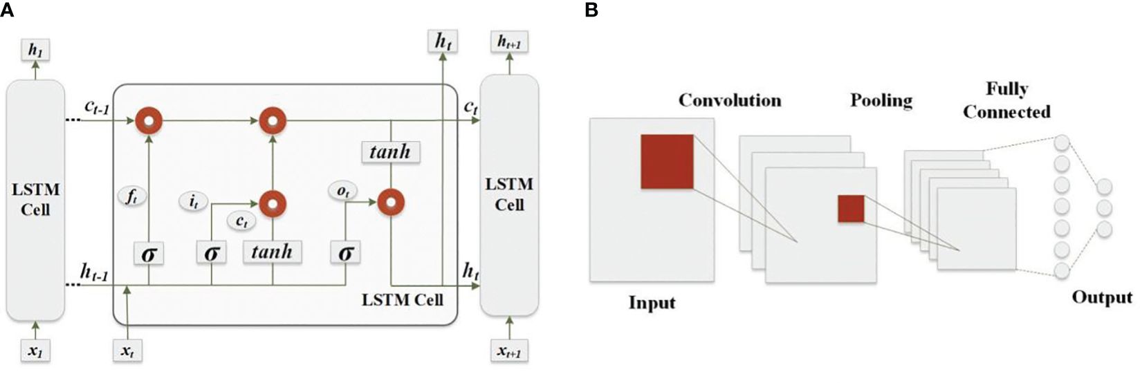
Figure 2 Schematics of different data-driven models: (A) LSTM model; (B) CNN model.

3.5.2 CNN

CNN, equipped with powerful data processing capabilities, consists of convolutional layers and pooling layers responsible for convolution calculations, feature extraction, and parameter sampling and compression (Mitiche et al., 2020). Utilizing weight sharing and local connectivity, the CNN model maps and processes the initial dataset, extracting relevant features to reduce parameter dimensions and improve computational speed. The principle involves employing multiple filters for feature extraction through layer-by-layer convolution and pooling operations on input data. These features are then converged in fully connected layers, addressing regression problems through activation functions.

The CNN structure, depicted in Figure 2B, comprises several components: an input layer for receiving raw data, a convolutional layer— the core module that extracts features via convolution operations, an activation function that introduces non-linear transformations to enhance model capacity, a pooling layer that reduces dimensionality while preserving key features, a fully connected layer that flattens the pooling layer’s output into a one-dimensional vector, connecting it to the output layer, and finally, an output layer that generates final model predictions.

3.6 Evaluation indicators

Different models’ predictive imputation performance is primarily assessed using specific evaluation metrics. Since there isn’t a universally applicable standard, multiple metrics are typically calculated to gauge a model’s generalization ability. To compare the predictive accuracy of various models, this study employs Root Mean Square Error (RMSE), Mean Absolute Error (MAE), and the coefficient of determination (R²) as evaluation metrics for model performance.

RMSE measures the disparity between predicted and observed values by averaging squared errors and then taking their square root to ensure non-negativity. MAE indicates prediction accuracy by averaging absolute prediction errors, reflecting how predictions deviate from true values. R² describes the goodness of fit, showcasing the model’s ability to explain data variability, with higher values indicating better prediction accuracy. As shown in Table 1, y_obs represents the observed values, y_f represents the predicted values, $\overline{y_{obs}}$ represents the mean of the observed values, and n is the number of observed values.

Table 1

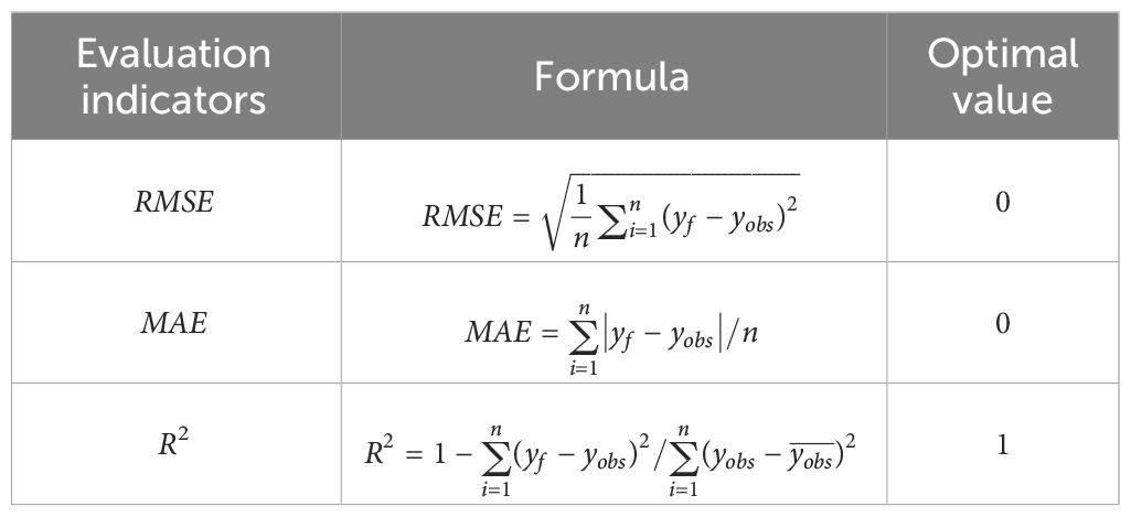
Table 1 Formulas of evaluation indicators.

4 Results

4.1 Missing data imputation

Due to missing data in the chlorine content from automatic monitoring stations, the study evaluated three imputation methods by introducing 5%, 10%, and 20% random missing data in the chlorine content data from six stations for October 2017 to February 2018. The imputation accuracy was assessed using RMSE, MAE, and R². Results in Table 2 and Figure 3 showed a consistent trend: lower missing ratios led to better imputation accuracy. For the median imputation method, when the missing ratio was 5%, the R² was 0.947, when the missing ratio was 10%, the R² was 0.882, and when the missing ratio was 20%, the R² was 0.732. The KNN method and the multiple imputation method showed the same law. It was worth noting that the multiple imputation method consistently outperformed other methods in different missing ratios. For example, when the missing ratio was 5%, RMSE of median method was 0.044, MAE was 0.006, R² was 0.947, RMSE of KNN method was 0.020, MAE was 0.002, R² was 0.989, RMSE of multiple inputation method was 0.015, MAE was 0.002, R² was 0.993. When the missing ratio was 10% and 20%, the R² of multiple imputation method was still the highest and the precision was the best.

Table 2

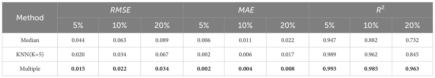
Table 2 Missing data imputation results.

Figure 3

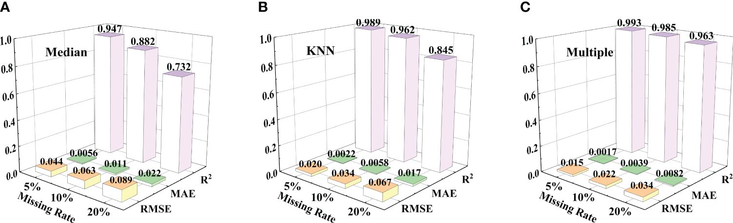
Figure 3 Comparison of index results of three imputation methods. (A) Median; (B) KNN; (C) Multiple.

Hence, this study enhanced accuracy by introducing new rules based on multiple imputation. For instance, if the upstream station (far from the estuary) exceeded the water supply chlorine limit (250mg/L), the chlorine content at the interpolated station was assuredly greater than 250mg/L. Additionally, if both upstream and downstream stations were (not) exceeding the limit, then the chlorine content at the interpolated station was greater than (less than) 250mg/L.

Due to the large dataset, only partial missing data periods are shown in Figure 4A, with black squares indicating missing values. During October 1-9, 2016, chloride data at NZ, XHW, and QL stations were entirely missing. From October 9-14, 2016, chloride data at QL station were missing. Interpolated data for some periods were displayed in Figure 4B, where missing values were filled. To illustrate the interpolation effect, data from October 1-14, 2016, were magnified in Figure 4C. It’s evident that missing data were effectively filled, aligning with the salinity boundary: chloride concentrations exceeded 250 mg/L below it and were below 250 mg/L above it.

Figure 4

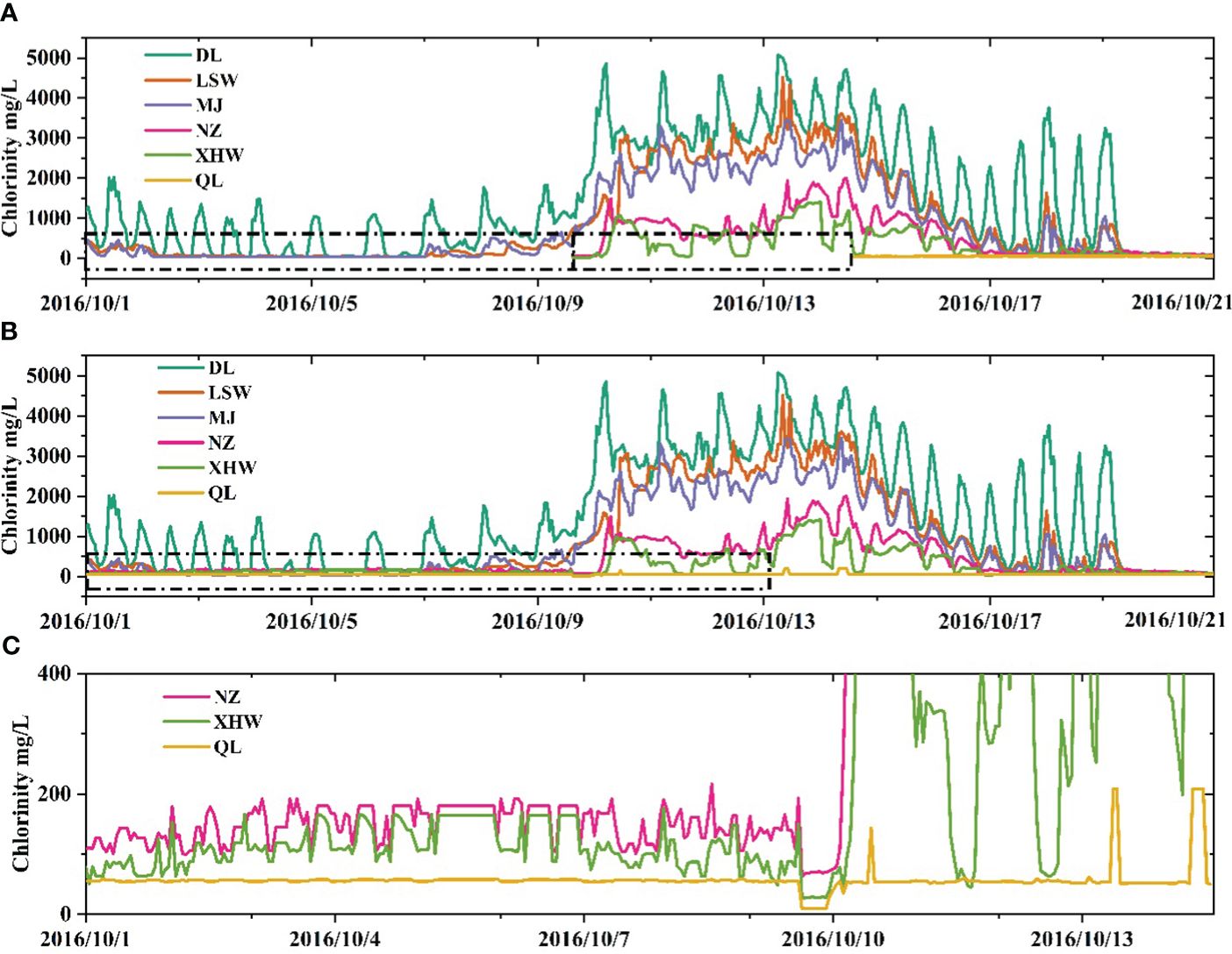
Figure 4 Interpolation effectiveness of chloride data imputation for missing values, (A) represents partially missing data, with black boxes representing missing values; (B) represents the interpolation results of the missing data in this part; (C) represents a partial amplification of the interpolation result.

4.2 Interannual variation in daily excessive duration at six stations

The time series in Figure 5 illustrates the interannual variability of daily excessive duration, denoting periods saltwater intrusion exceeds the water supply chlorine limit of 250mg/L in the MDM waterway from 2016 to 2020. Stations 1-6 represent downstream to upstream locations: DLS, LSW, MJ, NZ, XHW, and QL, respectively. Notably, the most severe intrusion occurred in 2019-2020, followed by 2016-2017, 2017-2018, and 2018-2019, showcasing significant yearly fluctuations.

Figure 5

Figure 5 The time series of daily excessive duration at the six stations. (The color bar represents the duration of chloride concentration exceeding standards within a day, with the color becoming increasingly red as the duration of the exceedance increases). (A) 2016-2017; (B) 2017-2018; (C) 2018-2019; (D) 2019-2020.

EOF analysis was performed to unveil the primary temporal and spatial patterns of daily excessive duration from 2016 to 2020. The first temporal mode (PC1), which accounted for 89% of the variation in daily excessive duration, was a crucial indicator for reflecting the temporal dynamics of saltwater intrusion (Table 3).

Table 3

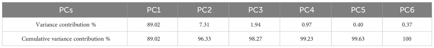
Table 3 Six principal components (PCs) obtained by EOF decomposition.

Figure 6A highlighted a notable increase in PC1 values during 2019-2020, signifying a phase of intensified saltwater intrusion and the longest excessive duration. Conversely, PC1 values were 0 in early October 2017 and March 2019, indicating periods with minimal or no saltwater intrusion and shorter excessive durations, aligning with the patterns observed in Figure 5. Figure 6B depicted a gradual decline in chlorine content from DLS to MJ, followed by a sharp decrease from MJ to upstream stations. This abrupt change could be attributed to a sudden increase in distance between neighboring stations, leading to a significant morphological shift. This suggested that MJ station plays a crucial role in assessing the extent of saltwater intrusion.

Figure 6

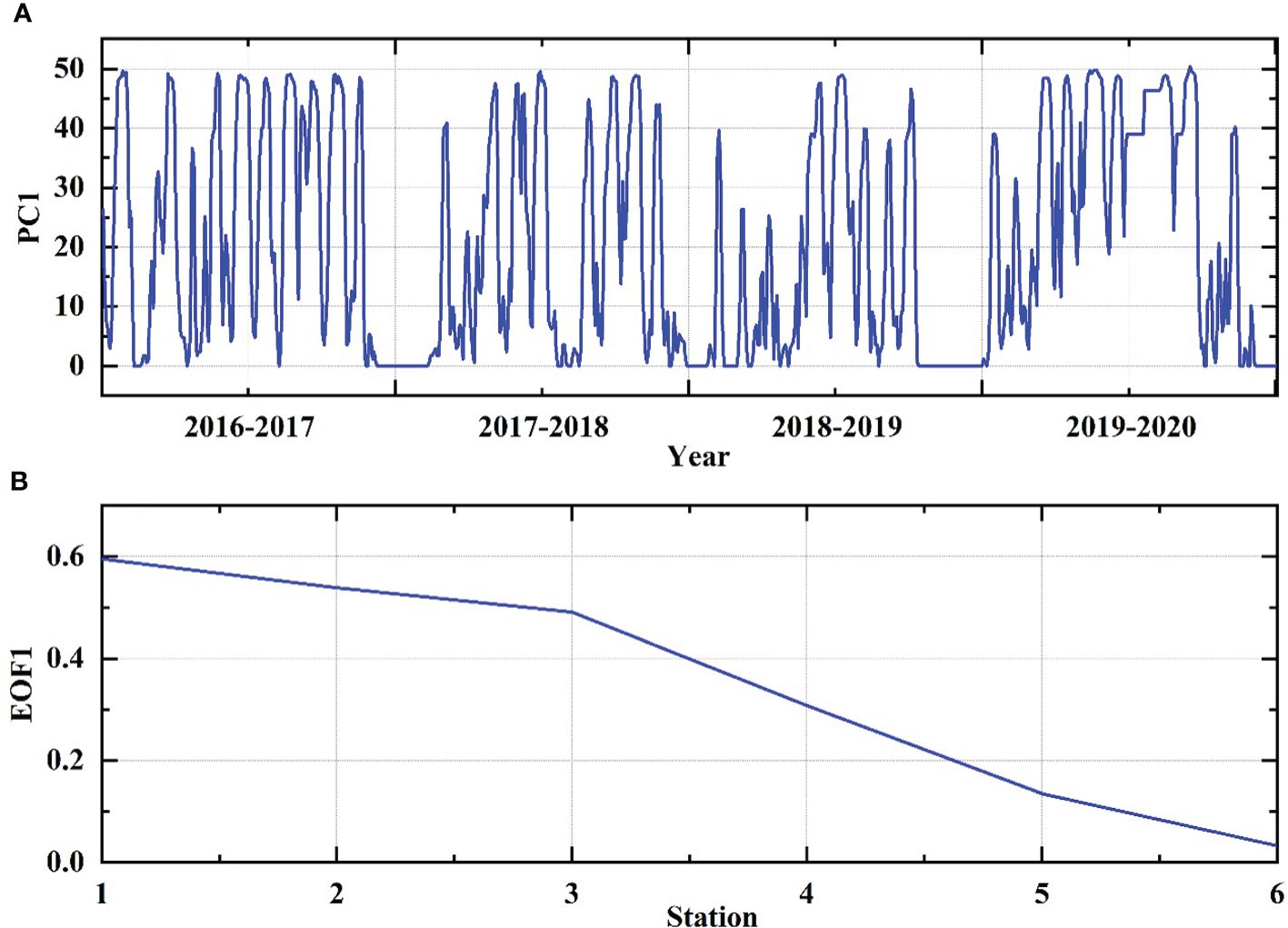
Figure 6 EOF decomposition plot of daily excessive duration, (A) first temporal mode and (B) first spatial mode.

Based on the analysis, this study used the first principal component (PC1) as a representation of saltwater intrusion distance. Research suggested that longer intrusion distances led to longer durations of exceeding standards, posing greater risks to water safety. The disaster threshold for chloride monitoring stations within 24 hours was 18 hours. When the duration of exceeding standards at a station ranged from 0 to 18 hours, it indicated saltwater intrusion without causing a disaster. The corresponding PC1 value for this intrusion extent was listed in Table 4. For intrusion distances between LSW and MJ, PC1 showed a small variation range, consistent with the spatial variation of the duration of exceeding standards shown in Figure 6B, confirming PC1’s effectiveness. When the intrusion distance was above XHW station, although PC1’s variation range was small, it still indicated saltwater intrusion severity. Below the XHW station, PC1 values showed a distinct range, enabling accurate intrusion distance prediction. PC1 exceeding 36 indicated a severe intrusion stage, identifying NZ station as another crucial site for assessing saltwater intrusion extent.

Table 4

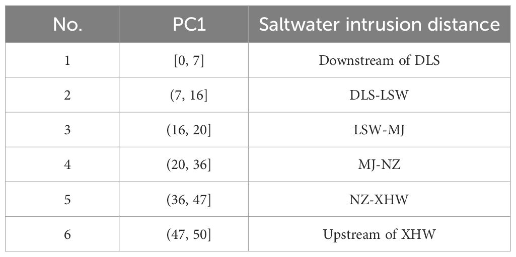
Table 4 Relationship between PC1 and saltwater intrusion distance.

To vividly depict the spatial changes in saltwater intrusion in the MDM waterway, we had selected MJ and NZ stations as pivotal sites reflecting intrusion severity. Table 5 below outlined the PC1 value divisions: PC1 ≤ 7 indicated intrusion downstream of DLS, 7<PC1 ≤ 20 suggested intrusion between DLS and MJ, 20<PC1 ≤ 36 signified intrusion between MJ and NZ, and PC1>36 denoted intrusion upstream of NZ.

Table 5

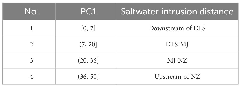
Table 5 Relationship between PC1 and saltwater intrusion distance.

4.3 Analysis of factors influencing saltwater intrusion and its temporal lag

As shown in Figure 7, PC1 illustrated the annual and monthly variations of saltwater intrusion during the dry season. It also depicted the sum of runoff at MK and SS stations, the daily maximum tidal range at SZ station, and wind conditions at Macao station. MDM, a typical river-dominated estuary, experiences variations in salinity primarily driven by changes in river discharge. An increase in discharge leaded to a decrease in PC1, and vice versa. The negative correlation between river discharge and saline water intrusion was evident, with PC1 changes lagging behind river discharge variations by several days (Figure 7B). The magnitude of tidal range is a key indicator of tidal strength. The daily maximum tidal range exhibits periodic variations, primarily on a half-month timescale. The interannual variation in tidal range was minimal, while the intra-annual variation was relatively larger, as shown in Figure 7C. The mean value of the daily maximum tidal range was 1.50 m. Figure 7D revealed substantial daily fluctuations in both wind speed and direction, with comparatively minor changes observed on a monthly scale. According to the daily wind rose plot (Figure 8), during the dry season at the MDM estuary, easterly winds prevailed at 37%, followed by southeast winds at 25%, and south winds at 13%. Additionally, southwest winds were at 10%, west winds at 5%, northeast winds at 6%, and other wind directions contributed 4%. This highlighted a predominant influence of easterly and southeast winds in the region. Generally, prevailing winds include both alongshore (parallel to the coastline) and cross-shore (perpendicular to the coastline) components, jointly influencing seawater intrusion. For instance, the alongshore component of easterly winds (southeast winds) enhances seawater intrusion, while its cross-shore component (northeast winds) diminishes seawater intrusion. As winds blow from south to north, aligning with estuarine tidal flow, they significantly increase salt transport, leading to pronounced seawater intrusion. This makes the estuary susceptible to short-term seawater intrusions near the estuary mouth, with a relatively minor impact on upstream river channels closer to inland areas.

Figure 7

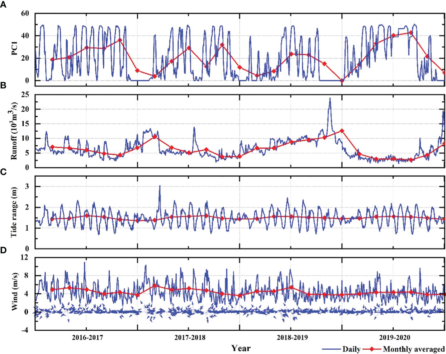
Figure 7 Time series of different characteristic variables, (A) PC1; (B) Runoff; (C) Tide range; (D) Wind.

Figure 8

Figure 8 Wind rose diagrams during the dry season from 2016 to 2020. Winds are divided into sixteen directions. The circle denotes the wind frequency of different directions. (A) 2016-2017; (B) 2017-2018; (C)2018-2019; (D) 2019-2020.

In this study, CART was employed to assess the significance and contributions of factors influencing salinity intrusion in the MDM estuary from 2016 to 2020. According to Figure 9, runoff had the most substantial impact (40%), followed by maximum tidal range, wind speed, and wind direction, contributing 25%, 20%, and 15%, respectively.

Figure 9

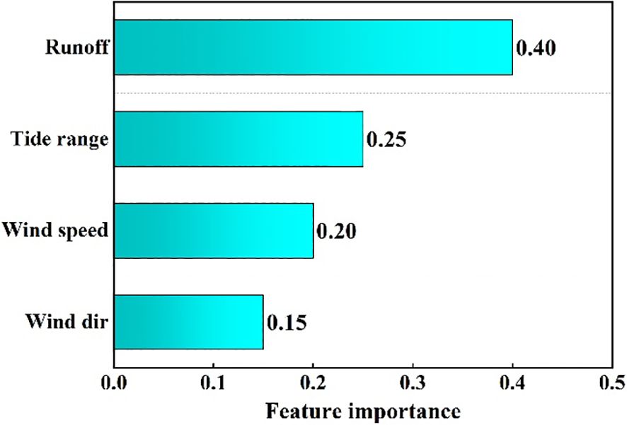
Figure 9 Contribution of influencing factors.

External forces are typically unstable, leading estuaries to exist in a non-equilibrium state when subjected to continuous changes. This dynamic state is characterized by a certain time lag effect (Liu et al., 2014; Gong et al., 2022). This study utilized Pearson correlation analysis to determine the time lag of salinity intrusion concerning various influencing factors. The results presented in Table 6 indicated that salinity intrusion in the MDM waterway lagged behind runoff by 1 day, tidal range by 3 days, and wind by 2 days. The maximum correlation coefficients were -0.457, -0.324, and 0.140, respectively, passing a 1% significance test. Furthermore, salinity intrusion demonstrates a significant negative correlation with runoff and maximum tidal range, while exhibiting a significant positive correlation with wind.

Table 6

Table 6 Correlation coefficient between PC1 and lag time of various influencing factors.

4.4 Cross-wavelet analysis of saltwater intrusion upstream

Saltwater intrusion is influenced by climatic changes, human activities, and topography, as well as atmospheric circulation factors. Research suggested (Wang et al., 2024) that cross-wavelet analysis could accurately reveal the relationship between atmospheric circulation and watershed climate changes, enhancing climate diagnostics and predictions. Saltwater intrusion in the MDM waterway was primarily driven by runoff dynamics, with upstream runoff contributing 40%. The WZ station, located in the middle and lower reaches of the Xijiang River basin, played a crucial role as a control point. Its flow rate determined the availability of water for regulating salinity and replenishing freshwater at the Pearl River Estuary. Using the cross-wavelet method, we investigated the main drivers of monthly runoff variations at WZ from 1961 to 2020, focusing on atmospheric circulation factors. Additionally, we analyzed the common characteristics between monthly runoff and nine atmospheric circulation factors (ENSO, PDO, NAO, AO, AMO, DMI, NPI, PNA, SSI) to infer the influence of atmospheric circulation on saltwater intrusion evolution.

Figure 10 depicted the cross-wavelet transform plot of monthly runoff at WZ station and atmospheric circulation factors in the low-energy region, i.e., the wavelet coherence spectrum. Color bars denoted the square of the wavelet coherence, with higher values indicating stronger correlation between the two-time series in the corresponding local time-frequency domain. The Figure 10 revealed a significant positive correlation between runoff and ENSO, spanning from 1973 to 1995 with a period of 128-190 months. Regarding PDO, six significant periods emerged: positive correlations from 1972 to 1976, 2002 to 2006, and 2011 to 2014 (8-16 months), and negative correlations from 1983 to 1987, 1993 to 1996, and 1998 to 2002 (8-16 months). As for NAO, notable periods included positive correlations from 1968 to 1972 and 1991 to 2010 (8-16 and 100-128 months, respectively), and negative correlations from 1967 to 1972 and 1991 to 1995, and 2011 to 2015 (24-40 and 8-16 months, respectively). Runoff demonstrated two significant resonance periods positively correlated with AO: 9-16 months during 1962-1968 and 24-30 months during 1987-1996. Regarding AMO, three notable resonance periods emerged: positive correlations during 1990-2000 (48-64 months) and 2002-2016 (8-20 months), and negative correlation during 1985-1998 (90-120 months). Two significant resonance periods negatively correlated with DMI were observed for runoff: 8-16 months during 1968-1972 and 18-40 months during 1964-1975. Concerning NPI, three significant resonance periods were identified: positive correlations during 1961-2020 (8-16 months), 2009-2015 (24-48 months), and negative correlation during 1976-2002 (128-256 months). Runoff exhibited four significant resonance periods negatively correlated with PNA: 8-16 months during 1982-1986, 1992-1995, 1998-2003, and 2008-2011. Lastly, with SSI, three significant resonance periods were identified: positive correlations during 1995-2001 (32-48 months) and 2002-2006 (10-16 months), and negative correlation during 1995-2005 (110-128 months).

Figure 10

Figure 10 The wavelet coherence spectrum plot. (The area within the cone-shaped contour lines indicates the effective spectral value influenced by the wavelet; the solid black line inside the cone represents the confidence interval passing the 95% significance level; arrows indicate phase difference, with rightward arrows indicating consistent phase changes between the two time series, and leftward arrows indicating opposite phase changes. The description is consistent with that of Figure 11).

Figure 11 showed the wavelet power spectrum of monthly runoff at WZ station and monthly-scale atmospheric circulation factors from 1961 to 2020. The color bars represented the power spectrum values, indicating the strength of signal oscillations and the significance of the corresponding period. Both runoff and atmospheric circulation factors exhibited short-term oscillation periods of 8-16 months, with NPI showing the strongest positive correlation with runoff. Additionally, short-term oscillation periods of 1-8 months were observed between runoff and atmospheric circulation factors during this period.

Figure 11

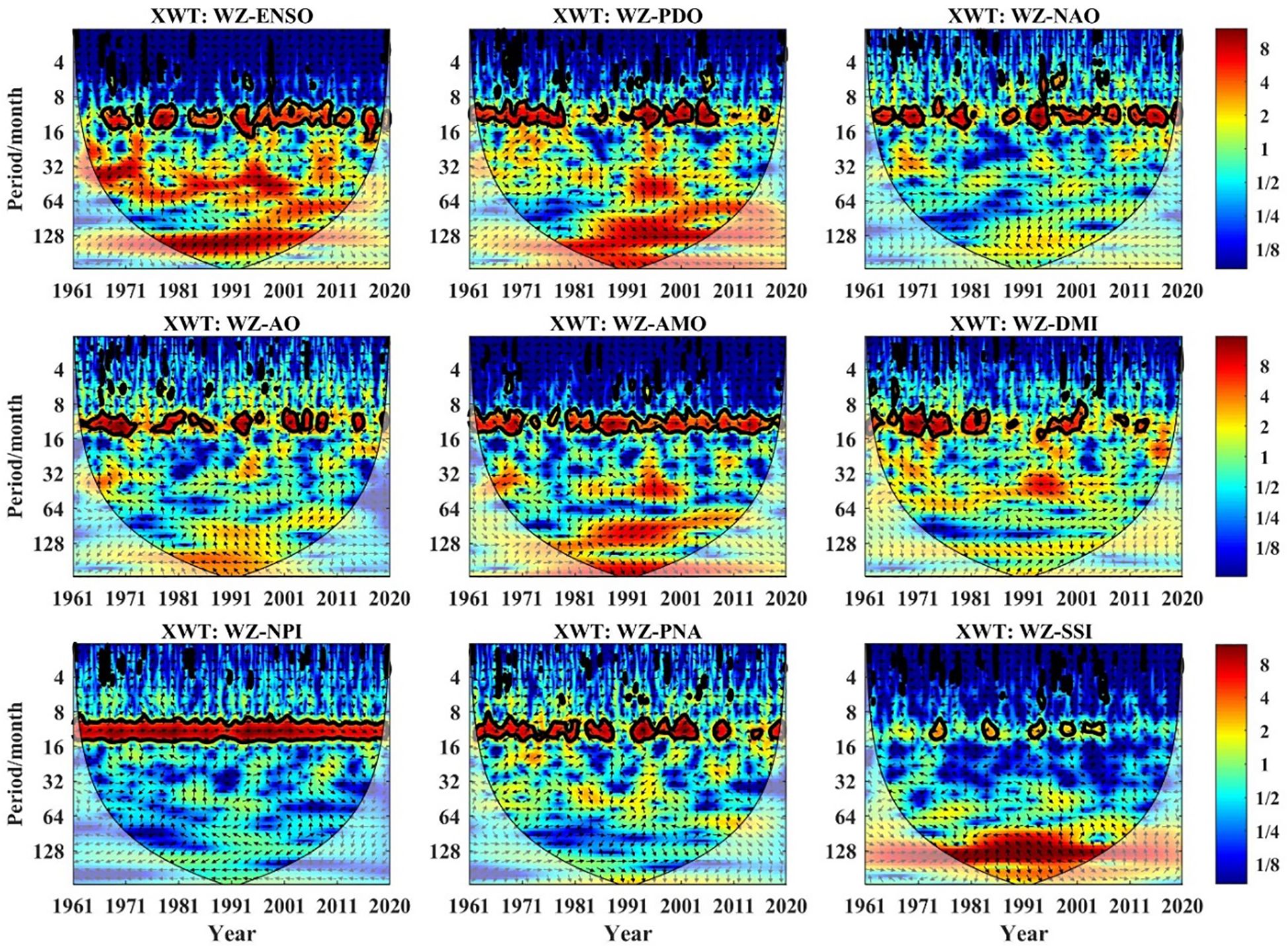
Figure 11 The wavelet power spectrum plot.

NPI, a crucial factor in ocean-atmosphere interaction and climate prediction, reflected sea-level pressure anomaly sensitivity, aiding in characterizing North Pacific climate system decadal variability. Given the inseparable link between saltwater intrusion and climate, NPI could enhance saltwater intrusion forecasting accuracy if integrated into early warning systems.

4.5 Prediction of saltwater intrusion distance

Considering the complexity of establishing separate daily exceedance duration prediction models for each of the six chlorine monitoring stations, it becomes challenging to provide an intuitive representation of the overall salinity intrusion process. Additionally, this approach would entail a substantial workload. Using the six PCs from EOF decomposition for prediction and multiplying them by spatial vectors enables the inverse estimation of the daily chlorine exceedance duration for all stations. Nevertheless, this approach still necessitates the development of six distinct prediction models, and the cumulative forecasting errors may introduce instability to the results. Based on the analysis, PC1, contributed to 89.02% of cumulative variance, effectively characterized the impact of various factors on salinity intrusion and its severity. Therefore, using PC1 as a predictive variable established a single forecasting model, reducing the need for multiple models and avoiding the randomness and instability associated with individual site data.

Model parameter selection significantly impacts prediction outcomes. In this study, parameters were chosen using a controlled variable approach to prevent overfitting of the training set and enhance the generalization ability of the test set. Optimal parameters within predefined ranges were presented in Table 7.

Table 7

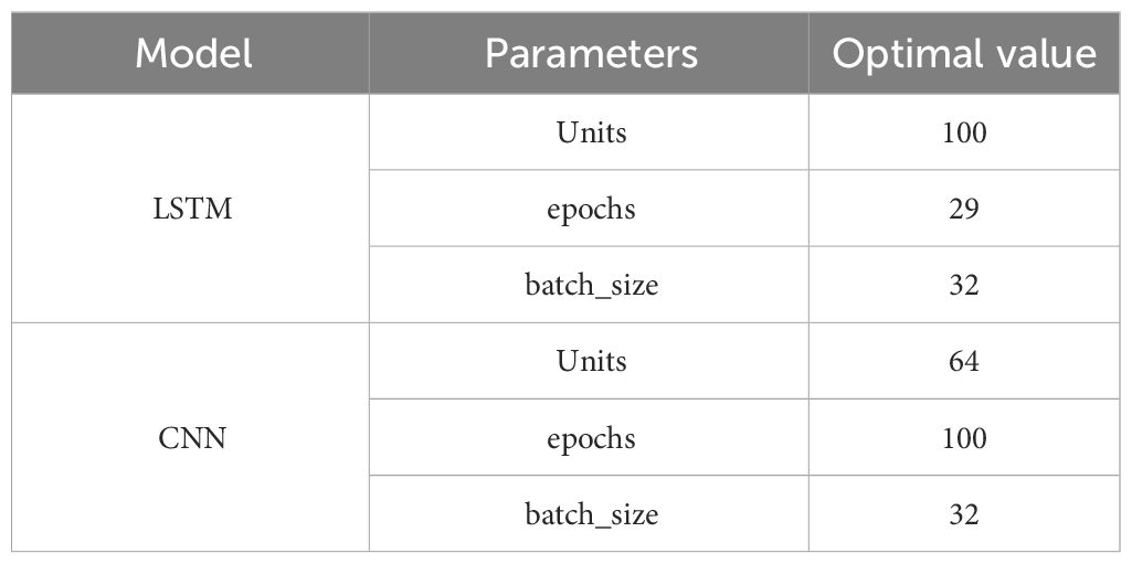
Table 7 Optimal parameters of the model.

LSTM and CNN methods were used to preliminarily assess the impact level of salinity intrusion (PC1) in the MDM waterway. Input variables included the 1-day lagged runoff sum of MK and SS, the 3-day lagged maximum tidal range at SZ, and the 2-day lagged wind speed at Macao station. The data were split into an 80% training set and a 20% validation set for model training. Results are shown in Figure 12 and Table 8.

Figure 12

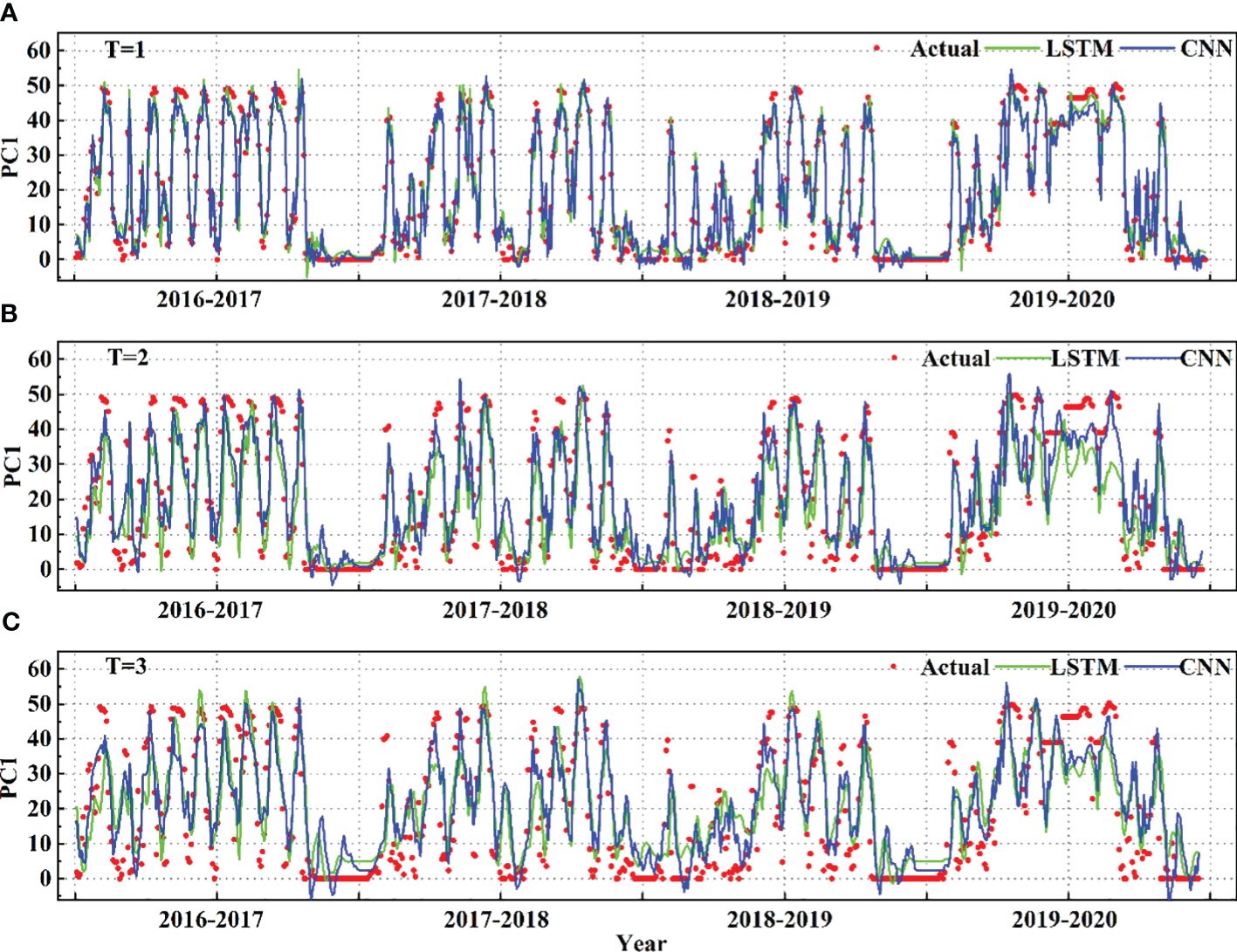
Figure 12 Comparison between predicted and actual values of the principal component PC1, which characterizes the extent of saltwater intrusion, at different forecast horizons. (A) T=1-day; (B) T=2-day; (C) T=3-day.

Table 8

Table 8 Model evaluation results.

With a 1-day horizon, LSTM performed best, achieving a test set RMSE of 6.57, MAE of 4.73, and R² of 0.89. Extending the horizon to 2 days, CNN outperformed. Compared to the 1-day horizon, LSTM’s test set saw a 94% increase in RMSE, 120% in MAE, and a 54% decrease in R². For CNN’s test set, there was a 50% increase in RMSE, 63% in MAE, and a 20% decrease in R². With a 3-day horizon, CNN maintained superiority. Compared to the 2-day horizon, LSTM’s test set experienced a 4% increase in RMSE, 5% in MAE, and a 6% decrease in R². Meanwhile, CNN’s test set showed a 5% increase in RMSE, 2% in MAE, and a 7% decrease in R². As the forecast horizon increased, model accuracy diminished to some extent. The reduction in accuracy for a 3-day horizon was smaller than for a 2-day horizon, exhibiting a decreasing trend. This is likely due to the nonlinear and time-delay characteristics of hydrological factors. Predicting salinity intrusion involves considering the interactions and delayed responses among various factors. As the forecast horizon extends, the model’s understanding of these complexities decreases. Additionally, a comparison between training and test sets revealed no overfitting, indicating the CNN model’s good generalization ability. Unlike the LSTM model, the CNN model maintained stable performance with an extended forecast horizon.

While both models exhibited reduced accuracy in predicting specific values of PC1 with an extended forecast horizon, Table 8 indicated that different intervals of PC1 effectively capture the impact of various factors on salinity intrusion and its severity. Both LSTM and CNN models performed well in predicting PC1 interval values. In terms of assessing the severity of salinity intrusion in the MDM waterway, these models maintained practicality and reliability.

5 Discussion

5.1 Possible causes of saltwater intrusion

5.1.1 The impact of tidal levels

The Pearl River estuary, characterized by multiple outlets, exhibits diverse tidal dynamics and variations in riverbed topography. Even within a single outlet, different mechanisms of salinity intrusion and stratification processes can occur under varying tidal conditions. As shown in Figure 13, salinity intrusion displayed a distinctive fortnightly tidal cycle. During neap tides, salinity intrusion intensified, reaching its peak shortly after the neap tide and weakening during spring tides. This is because during the neap tide, gravitational circulation stratifies saline and fresh water, with the saltwater wedge advancing from the bottom. In the post-neap to mid-tide phase, vertical mixing intensifies, leading to enhanced mixing and a maximum upstream distance. During the spring tide, gravitational circulation and river runoff interaction strengthen saline and fresh water mixing, resembling a “piston” effect. The saltwater-freshwater interface moves downward. Consequently, the maximum salinity intrusion typically occurs between neap tides and spring tides, while the minimum intrusion usually occurs during spring tides.

Figure 13

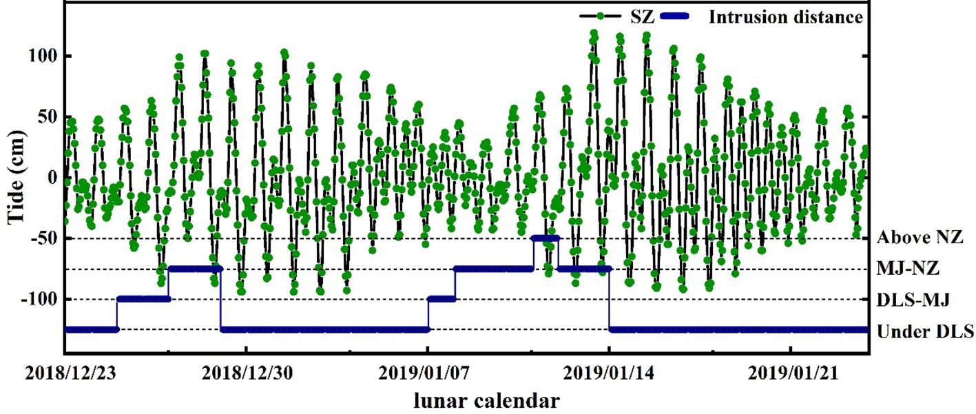
Figure 13 The process of salinity intrusion distance and the tidal level variation at the SZ station.

5.1.2 The impact of wind

In this paper, wind component was obtained through calculation of wind speed and direction. Although wind component is also a factor affecting seawater intrusion, in practical applications, observation data of wind speed and direction are relatively easy to obtain with high observation accuracy, which is more in line with the needs of practical applications. However, calculation of wind component may introduce additional errors. Wind speed and wind direction directly reflect the influence of wind intensity and direction on seawater intrusion. Choosing them as the driving factors of brine intrusion may help simplify the model and improve the interpretability of the model. Therefore, wind speed and wind direction were chosen as the driving factors of brine intrusion in this paper (Li et al., 2012; Duan et al., 2021).

5.2 Uncertainty

This study faces uncertainty in three aspects. Firstly, the chlorine concentration data, sourced from automatic monitoring stations, could have had missing values during certain periods. Despite employing optimal interpolation methods and rigorous quality control, the filled values might not have precisely represent the actual concentrations at those times, introducing potential uncertainty into the assessment of salinity intrusion severity and subsequent analyses. Secondly, in using LSTM and CNN to predict the time series (PC1) representing salinity intrusion severity, the choice of model parameters significantly influenced the forecasting results. The parameters selected in this study were optimized within a specified range to prevent overfitting in the training set while maximizing generalization ability on the test set. However, the existence of superior parameters beyond this range remains unknown. Finally, the upwelling of salt tides in the Pearl River estuary has a typical half-moon tidal cycle variation law. Meanwhile, according to the cross wavelet analysis by Gong et al. (2022), it can be seen that the saltwater intrusion variation of MDM waterway has a resonance period of 12-17 days with the tidal range of SZ station, and the half-moon cycle in this paper is precisely concentrated in this range. During model training, a training time window of 15 days was selected, and the model performance and results were also obtained by training under this window. The training time window was of the preset size, so the model effect outside this selection was not yet known.

5.3 Advantages and limitations

The combined EOF and neural network trend prediction method simplified multidimensional data, effectively capturing the spatial variation of daily exceedance time at six chlorine monitoring stations in the MDM waterway. Using the PC1 obtained from EOF decomposition as a predictive variable, a single forecasting model was established to determine salinity intrusion severity. Therefore, when other estuarine areas, such as the Rhine-Meuse Delta, have multiple chlorine monitoring stations, the EOF decomposition method can also be used to identify key factors reflecting the spatiotemporal variations of saltwater intrusion. These factors can then be predicted to forecast the severity of saltwater intrusion.

Extreme events such as tropical cyclones and cold fronts will also have a certain impact on salt intrusion. Refer to Zhu et al. (2020), only northerly winds with wind speeds greater than 10 m/s can cause net transport to land in the northern Channel, and extremely serious seawater intrusion will occur only when northerly winds last for 8 days. However, the duration of the northerly wind induced by the cold front was only 1-2 days, and no extremely serious seawater intrusion event occurred. According to the study area and data period of this paper, extreme weather events such as autumn tropical cyclones (typhoons) did not occur during 2016-2020, and MDM is a typical estuary with strong diameter and weak tide. When the upstream flow is very small, strong seawater intrusion events have already occurred in the downstream estuary, which has little impact on the overall saltwater intrusion in the estuary. In future studies, we can try to take into account the effects of these extreme events in the regions where they exist and in the data cycle.

6 Conclusion

This study first utilized multiple imputation to address missing chlorine concentration data. Subsequently, it applied methods like EOF decomposition, decision trees, and neural network time series prediction to analyze the variation patterns and key factors influencing salinity intrusion in the MDM waterway during the dry season from 2016 to 2020. Finally, the study predicted the severity of salinity intrusion. The key findings included:

(1) The first temporal mode (PC1), derived from EOF decomposition, accounted for 89% of daily chlorine exceedance time, effectively reflecting temporal changes in salinity intrusion. A higher PC1 value indicated more severe salinity intrusion. Specifically, when 0≤PC1 ≤ 7, the saltwater boundary was below DLS station; when 7<PC1 ≤ 20, it lay between DLS and MJ stations; when 20<PC1 ≤ 36, it was between MJ and NZ stations; and when 36<PC1 ≤ 50, it was above NZ station. The first spatial mode (EOF1) explained the spatial variation in daily exceedance time, with a gradual decrease from DLS station to MJ station and a sharp decline from MJ to upstream stations.

(2) The primary factor impacting salinity intrusion in the MDM waterway was runoff, contributing 40%. Subsequently, maximum tidal range, wind speed, and wind direction follow with contributions of 25%, 20%, and 15%, respectively. Salinity intrusion exhibited a lag of 1 day with runoff, 3 days with tidal range, and 2 days with wind. Notably, it showed a significant negative correlation with runoff and maximum tidal range (correlation coefficients of -0.457 and -0.324) and a positive correlation with wind (correlation coefficient of 0.140), passing a 1% significance test. NPI had the strongest positive correlation with saltwater intrusion among the 9 atmospheric circulation factors.

(3) When predicting the time series PC1 that represents the severity of salinity intrusion, LSTM achieved the highest accuracy with an R² of 0.89 for a horizon of 1 day. For horizons of 2 days and 3 days, CNN exhibited the highest accuracy with R² values of 0.73 and 0.68, respectively. Although the precision of both models in predicting specific values of PC1 decreased with an extended forecast horizon, they still demonstrated practicality and reliability in assessing the severity of salinity intrusion in the MDM waterway.

Data availability statement

The data analyzed in this study is subject to the following licenses/restrictions: The raw data supporting the conclusions of this article will be made available by the authors, without undue reservation. Requests to access these datasets should be directed to Yu Tian, ty10078@126.com.

Author contributions

QT: Conceptualization, Data curation, Investigation, Writing – original draft. HG: Data curation, Formal analysis, Investigation, Methodology, Validation, Writing – original draft. YT: Conceptualization, Investigation, Methodology, Visualization, Writing – review & editing. QW: Data curation, Investigation, Methodology, Writing – original draft. LG: Conceptualization, Resources, Writing – original draft. QC: Conceptualization, Writing – original draft.

Funding

The author(s) declare financial support was received for the research, authorship, and/or publication of this article. This research was supported by National Key Research and Development Program of China (2021YFC3001000), the Open Research Fund of State Key Laboratory of Simulation and Regulation of Water Cycle in River Basin, China Institute of Water Resources and Hydropower Research (IWHR-SKL-KF202207), and Yinshanbeilu Grassland Eco-hydrology National Observation and Research Station, China Institute of Water Resources and Hydropower Research (YSS202118).

Acknowledgments

Furthermore, sincere thanks to editors and reviewers for putting forward guiding measures to improve the quality of this paper.

Conflict of interest

Author LG was employed by Henan Water Valley Innovation Technology Research Institute Co., LTD.

The remaining authors declare that the research was conducted in the absence of any commercial or financial relationships that could be construed as a potential conflict of interest.

Publisher’s note

All claims expressed in this article are solely those of the authors and do not necessarily represent those of their affiliated organizations, or those of the publisher, the editors and the reviewers. Any product that may be evaluated in this article, or claim that may be made by its manufacturer, is not guaranteed or endorsed by the publisher.

References

Anoek J. V. T., Hudson P. F. (2022). Extreme weather events and farmer adaptation in Zeeland, the Netherlands: A European climate change case study from the Rhine delta. Sci. Total Environ. 844, 157212. doi: 10.1016/j.scitotenv.2022.157212

PubMed Abstract | CrossRef Full Text | Google Scholar

Bae S. M. (2019). The prediction model of suicidal thoughts in Korean adults using decision tree analysis: a nationwide cross-sectional study. PloS One 14, e0223220. doi: 10.1371/journal.pone.0223220

PubMed Abstract | CrossRef Full Text | Google Scholar

Barzegar R., Aalami M. T., Adamowski J. (2020). Short-term water quality variable prediction using a hybrid CNN-LSTM deep learning mode. Stoch. Env. Res. Risk A. 34, 415–433. doi: 10.1007/s00477-020-01776-2

CrossRef Full Text | Google Scholar

Beesley L. J., Bondarenko I., Elliot M. R., Kurian A. W., Katz S. J., Taylor J. M. (2021). Multiple imputation with missing data indicators. Stat. Methods Med. Res. 30, 2685–2700. doi: 10.1177/09622802211047346

PubMed Abstract | CrossRef Full Text | Google Scholar

Björnsson H., Venegas S. A. (1997). A manual for EOF and SVD analyses of climatic data. CCGCR Rep. 97, 112–134.

Google Scholar

Chen S. N. (2015). Asymmetric estuarine response to changes in river forcing: a consequence of nonlinear salt flux. J. Phys. Oceanogr. 45, 2836–2847. doi: 10.1175/JPO-D-15-0085.1

CrossRef Full Text | Google Scholar

Dahj J. N. M., Ogudo K. A. (2023). Machine learning-based imputation approach with dynamic feature extraction for wireless RAN performance data preprocessing. Symmetry 15, 1161. doi: 10.3390/sym15061161

CrossRef Full Text | Google Scholar

Das S., Hazra S., Haque A., Rahman M., Nicholls R. J., Ghosh A., et al. (2021). Social vulnerability to environmental hazards in the Ganges-Brahmaputra-Meghna delta, India and Bangladesh. Int. J. Disast. Risk Re. 53, 101983. doi: 10.1016/j.ijdrr.2020.101983

CrossRef Full Text | Google Scholar

Duan B., Zhang W., Yang X., Zhu M. (2021). Assimilation of ASCAT sea surface wind retrievals with correlated observation errors. J. Meteorol. Res-Prc. 35, 478–489. doi: 10.1007/s13351-021-1007-0

CrossRef Full Text | Google Scholar

Gao W. Y., Su C. (2020). Analysis on block chain financial transaction under artificial neural network of deep learning. J. Comput. Appl. Math. 380, 112991. doi: 10.1016/j.cam.2020.112991

CrossRef Full Text | Google Scholar

Gong W. P., Lin Z. Y., Zhang H., Lin H. Y. (2022). The response of salt intrusion to changes in river discharge, tidal range, and winds, based on wavelet analysis in the Modaomen estuary, China. Ocean Coast. Manage. 219, 106060. doi: 10.1016/j.ocecoaman.2022.106060

CrossRef Full Text | Google Scholar

Gong W., Shen J. (2011). The response of salt intrusion to changes in river discharge and tidal mixing during the dry season in the Modaomen Estuary, China. Cont. Shelf Res. 31, 769–788. doi: 10.1016/j.csr.2011.01.011

CrossRef Full Text | Google Scholar

Habib M. A., O’Sullivan J. J., Abolfathi S., Salauddin M. (2023). Enhanced wave overtopping simulation at vertical breakwaters using machine learning algorithms. PloS One 18, e0289318. doi: 10.1371/journal.pone.0289318

PubMed Abstract | CrossRef Full Text | Google Scholar

Hadeed S. J., O’Rourke M. K., Burgess J. L., Harris R. B., Canales R. A. (2020). Imputation methods for addressing missing data in short-term monitoring of air pollutants. Sci. Total Environ. 730, 139140. doi: 10.1016/j.scitotenv.2020.139140

PubMed Abstract | CrossRef Full Text | Google Scholar

Hoai P. N., Quoc P. B., Thai T. T. (2022). Apply machine learning to predict saltwater intrusion in the ham Luong River, Ben Tre province. VNU J. Sci.: Earth Environ. Sci. 38, 79–92. doi: 10.25073/2588-1094/vnuees.4852

CrossRef Full Text | Google Scholar

Hochreiter S., Schmidhuber J. (1997). Long short-term memory. Neural Comput. 9, 1735–1780. doi: 10.1162/neco.1997.9.8.1735

PubMed Abstract | CrossRef Full Text | Google Scholar

Hu H. J., Chen G. D., Lin R., Huang X., Wei Z. D., Chen G. H. (2024). An observation study of the combined river discharge and sea level impact on the duration of saltwater intrusion in Pearl River estuary-Modaomen waterway. Nat. Hazards 120, 409–428. doi: 10.1007/s11069-023-06146-z

CrossRef Full Text | Google Scholar

Hu J. Y., Liu B. J., Peng S. H. (2019). Forecasting salinity time series using RF and ELM approaches coupled with decomposition techniques. Stoch. Env. Res. Risk A. 33, 1117–1135. doi: 10.1007/s00477-019-01691-1

CrossRef Full Text | Google Scholar

Hunter J. M., Maier H. R., Gibbs M. S., Foale E. R., Grosvenor N. A., Harders N. P., et al. (2018). Framework for developing hybrid process-driven, artificial neural network and regression models for salinity prediction in river systems. Hydrol. Earth Syst. Sc. 22, 2987–3006. doi: 10.5194/hess-22-2987-2018

CrossRef Full Text | Google Scholar

Kao I. F., Zhou Y. L., Chang L. C., Chang F. J. (2020). Exploring a Long Short-Term Memory based Encoder-Decoder framework for multi-step-ahead flood forecasting. J. Hydrol. 583, 124631. doi: 10.1016/j.jhydrol.2020.124631

CrossRef Full Text | Google Scholar

Karunarathna H., Horrillo-Caraballo J. M., Ranasinghe R., Short A. D., Reeve D. E. (2012). An analysis of the cross-shore beach morphodynamics of a sandy and a composite gravel beach. Mar. Geol. 299, 33–42. doi: 10.1016/j.margeo.2011.12.011

CrossRef Full Text | Google Scholar

Kratzert F., Klotz D., Brenner C., Schulz K., Herrnegger M. (2018). Rainfall-runoff modelling using long short-term memory (LSTM) networks. Hydrol. Earth Syst. Sc. 22, 6005–6022. doi: 10.5194/hess-22-6005-2018

CrossRef Full Text | Google Scholar

Lara–Benítez P., Carranza–García M., Riquelme J. C. (2021). An experimental review on deep learning architectures for time series forecasting. Int. J. Neural Syst. 31, 2130001. doi: 10.1142/S0129065721300011

PubMed Abstract | CrossRef Full Text | Google Scholar

Lathashri U. A., Mahesha A. (2015). Simulation of saltwater intrusion in a coastal aquifer in Karnataka, India. Aquat. Procedia 4, 700–705. doi: 10.1016/j.aqpro.2015.02.090

CrossRef Full Text | Google Scholar

Le X. H., Ho H. V., Lee G., Jung S. (2019). Application of long short-term memory (LSTM) neural network for flood forecasting. Water 11, 1387. doi: 10.3390/w11071387

CrossRef Full Text | Google Scholar

Li L., Zhu J., Wu H. (2012). Impacts of wind stress on saltwater intrusion in the Yangtze Estuary. Sci. China Earth Sci. 55, 1178–1192. doi: 10.1007/s11430-011-4311-1

CrossRef Full Text | Google Scholar

Lin Z. Y., Zhang H., Lin H., Gong W. P. (2019). Intraseasonal and interannual variabilities of saltwater intrusion during dry seasons and the associated driving forcings in a partially mixed estuary. Cont. Shelf Res. 174, 95–107. doi: 10.1016/j.csr.2019.01.008

CrossRef Full Text | Google Scholar

Liu B. J., Liao Y. Y., Yan S. L., Yan H. H. (2017). Dynamic characteristics of saltwater intrusion in the Pearl River Estuary. China Nat. Hazards 89, 1097–1117. doi: 10.1007/s11069-017-3010-4

CrossRef Full Text | Google Scholar

Liu P. Y., Lin K. R., Xu C. Y., lan T., Liu Z. Y., He Y. H. (2021). An integrated framework of input determination for ensemble forecasts of monthly estuarine saltwater intrusion. J. Hydrol. 598, 126225. doi: 10.1016/j.jhydrol.2021.126225

CrossRef Full Text | Google Scholar

Liu B. J., Yan S. L., Chen X. H., Lian Y. Q., Xin Y. B. (2014). Wavelet analysis of the dynamic characteristics of saltwater intrusion–a case study in the Pearl River Estuary of China. Ocean Coast. Manage. 95, 81–92. doi: 10.1016/j.ocecoaman.2014.03.027

CrossRef Full Text | Google Scholar

Loc H. H., Van Binh D., Park E., Shrestha S., Dung T. D., Son V. H., et al. (2021). Intensifying saline water intrusion and drought in the Mekong Delta: From physical evidence to policy outlooks. Sci. Total Environ. 757, 143919. doi: 10.1016/j.scitotenv.2020.143919

PubMed Abstract | CrossRef Full Text | Google Scholar

Mitiche I., Nesbitt A., Conner S., Boreham P., Morison G. (2020). 1D-CNN based real-time fault detection system for power asset diagnostics. IET Gener. Transm. Dis. 14, 5766–5773. doi: 10.1049/iet-gtd.2020.0773

CrossRef Full Text | Google Scholar

Pappa A., Dokou Z., Karatzas G. P. (2017). Saltwater intrusion management using the SWI2 model: application in the coastal aquifer of Hersonissos, Crete, Greece. Desalin. Water Treat. 99, 49–58. doi: 10.5004/dwt

CrossRef Full Text | Google Scholar

Park M., Choi S., Shin A. M., Koo C. H. (2013). Analysis of the characteristics of the older adults with depression using data mining decision tree analysis. J. Korean Acad. Nurs. 43, 1–10. doi: 10.4040/jkan.2013.43.1.1

PubMed Abstract | CrossRef Full Text | Google Scholar

Prayag A. G., Zhou Y. X., Srinivasan V., Stigter T., Verzijl A. (2023). Assessing the impact of groundwater abstractions on aquifer depletion in the Cauvery Delta, India. Agric. Water Manage. 279, 108191. doi: 10.1016/j.agwat.2023.108191

CrossRef Full Text | Google Scholar

Qiu C., Wan Y. S. (2013). Time series modeling and prediction of salinity in the Caloosahatchee River Estuary. Water Resour. Res. 49, 5804–5816. doi: 10.1002/wrcr.20415

CrossRef Full Text | Google Scholar

Ren G. (2021). Application of neural network algorithm combined with bee colony algorithm in English course recommendation. Comput. Intel. Neurosc. 2021, 1–9. doi: 10.1155/2021/5307646

CrossRef Full Text | Google Scholar

Rohmer J., Brisset N. (2017). Short-term forecasting of saltwater occurrence at La Comté River (French Guiana) using a kernel-based support vector machine. Environ. Earth Sci. 76, 1–16. doi: 10.1007/s12665-017-6553-5

CrossRef Full Text | Google Scholar

Sahoo A., Ghose D. K. (2022). Imputation of missing precipitation data using KNN, SOM, RF, and FNN. Soft Comput. 26, 5919–5936. doi: 10.1007/s00500-022-07029-4

CrossRef Full Text | Google Scholar

Shammi M., Rahman M. M., Bondad S. E., Bodrud-Doza M. (2019). Impacts of salinity intrusion in community health: a review of experiences on drinking water sodium from coastal areas of Bangladesh. Healthcare 7, 50. doi: 10.3390/healthcare7010050

PubMed Abstract | CrossRef Full Text | Google Scholar

Tang G. P., Yang M. Z., Chen X. H., Jiang T., Chen T., Chen X. H., et al. (2020). A new idea for predicting and managing seawater intrusion in coastal channels of the Pearl River, China. J. Hydrol. 590, 125454. doi: 10.1016/j.jhydrol.2020.125454

CrossRef Full Text | Google Scholar

Tian R. (2019). Factors controlling saltwater intrusion across multi-time scales in estu-aries, Chester River, Chesapeake Bay. Estuar. Coast. Shelf Sci. 223, 61–73. doi: 10.1016/j.ecss.2019.04.041

CrossRef Full Text | Google Scholar

Tian Q. Q., Gao. H., Tian Y., Jiang Y. Z., Li Z. X., Guo L. (2023). Runoff prediction in the Xijiang River Basin based on Long Short-Term Memory with variant models and its interpretable analysis. Water 15, 3184. doi: 10.3390/w15183184

CrossRef Full Text | Google Scholar

Wang F., Lai H. X., Men R. Y., Sun K., Li Y. B., Feng K., et al. (2024). Spatial and temporal evolutions of terrestrial vegetation drought and the influence of atmospheric circulation factors across the Mainland China. Ecol. Indic. 158, 111455. doi: 10.1016/j.ecolind.2023.111455

CrossRef Full Text | Google Scholar

Wijesuriya R., Moreno-Betancur M., Carlin J. B., Lee K. J. (2020). Evaluation of approaches for multiple imputation of three-level data. BMC Med. Res. Methodol. 20, 1–15. doi: 10.1186/s12874-020-01079-8

CrossRef Full Text | Google Scholar

Wullems B. J. M., Brauer C. C., Baart F., Weerts A. H. (2023). Forecasting estuarine salt intrusion in the Rhine-Meuse delta using an LSTM model. Hydrol. Earth Syst. Sc. 27, 3823–3850. doi: 10.5194/hess-27-3823-2023

CrossRef Full Text | Google Scholar

Xiao Y. C., Wang H. G., Xu W. L. (2014). Parameter selection of Gaussian kernel for one-class SVM. IEEE T. Cybernetics 45, 941–953. doi: 10.1109/TCYB.2014.2340433

CrossRef Full Text | Google Scholar

Yaseen Z. M., El-Shafie A., Jaafar O., Afan H. A., Sayl K. N. (2015). Artificial intelligence based models for stream-flow forecasting: 2000-2015. J. Hydrol. 530, 829–844. doi: 10.1016/j.jhydrol.2015.10.038

CrossRef Full Text | Google Scholar

Ye R. H., Song Z. Y., Zhang C. M., He Y., Yu S. C., Kong J., et al. (2017). Analytical model for surface saltwater intrusion in estuaries. J. Coast. Res. 33, 712–719. doi: 10.2112/JCOASTRES-D-16-00069.1

CrossRef Full Text | Google Scholar

Zhang E. F., Gao S., Savenije H. H. G., Si G. Y., Cao S. (2019). Saline water intrusion in relation to strong winds during winter cold outbreaks: North Branch of the Yangtze Estuary. J. Hydrol 574, 1099–1109. doi: 10.1016/j.jhydrol.2019.04.096

CrossRef Full Text | Google Scholar

Zhang S. C., Li X. L., Zong M., Zhu X. F., Wang R. L. (2017). Efficient kNN classification with different numbers of nearest neighbors. IEEE T. Neur. Net. Lear. 29, 1774–1785. doi: 10.1109/TNNLS.2017.2673241

CrossRef Full Text | Google Scholar

Zhang X. L., Peng Y., Zhang C., Wang B. D. (2015). Are hybrid models integrated with data preprocessing techniques suitable for monthly streamflow forecasting? Some experiment evidences. J. Hydrol. 530, 137–152. doi: 10.1016/j.jhydrol.2015.09.047

CrossRef Full Text | Google Scholar

Zhang Y., Xu L. H., Zhang Y. K. (2022). Research on hierarchical pedestrian detection based on SVM classifier with improved kernel function. Meas. Control 55, 1088–1096. doi: 10.1177/00202940221110164

CrossRef Full Text | Google Scholar

Zhou F. H., Liu B. J., Duan K. (2020). Coupling wavelet transform and artificial neural network for forecasting estuarine salinity. J. Hydrol. 588, 125127. doi: 10.1016/j.jhydrol.2020.125127

CrossRef Full Text | Google Scholar

Zhou X. D., Yang T., Shi P. F., Yu Z. B., Wang X. Y., Li Z. Y. (2017). Prospective scenarios of the saltwater intrusion in an estuary under climate change context using Bayesian neural networks. Stoch. Env. Res. Risk A. 31, 981–991. doi: 10.1007/s00477-017-1399-7

CrossRef Full Text | Google Scholar

Zhu J., Cheng X., Li L., Wu H., Gu J., Lyu H. (2020). Dynamic mechanism of an extremely severe saltwater intrusion in the Changjiang estuary in February 2014. Hydrol. Earth Syst. Sc. 24, 5043–5056. doi: 10.5194/hess-24-5043-2020

CrossRef Full Text | Google Scholar