
94% of researchers rate our articles as excellent or good
Learn more about the work of our research integrity team to safeguard the quality of each article we publish.
Find out more
ORIGINAL RESEARCH article
Front. Mar. Sci., 29 July 2024
Sec. Marine Fisheries, Aquaculture and Living Resources
Volume 11 - 2024 | https://doi.org/10.3389/fmars.2024.1407670
 Xiuchen Li1,2,3
 Yu Yang1
 Dongshuo Liu4Shuo Chen1Shuqiao Wu1Xiang Yuan1Zibo Liu1Yubao Wang1
 Hanbing Zhang1,2,3*
This article aims to address the issues of low cultivation density and high labor intensity of manual water exchange in existing scallop seedling ponds, an upwelling recirculating water system for scallop larval cultivation is designed. EDEM-Fluent coupled model was used to simulate the movement of scallop larvae in the culture cone in order to guarantee the uniform distribution of larvae in the cultivation device. Design-Expert software was utilized to investigate the impact of the bottom cone angle(θ), the column height/cone height ratio(n) and the inflow velocity(v) on the variation coefficients of the axial and radial distributions of D-shaped larvae within the culture cone. The results indicated that θ = 108.97° and n = 1.8 represent the ideal structural parameters for the culture cone. The further investigation of the culture cones prototype was conducted to examine the impact of the inlet deflector angle (α), cultivation density (τ), and inflow velocity (v) on its performance. θ=108.97°, n=1.8, v=0.19m/s, α=60.94°, and τ=110pcs/ml were found to be the ideal combination of parameters, in this scenario, the D-shaped larvae’s radial distributions’ coefficients of variation is 22.13%, the error between the experimental and simulation results is 4.41%. Research has shown that EDEM-Fluent based simulation analysis methods can be used for the design and parameter optimization of upwelling recirculating water scallop larval cultivation system, this paper can provide a reference for the design of an upwelling recirculating water scallop larval cultivation system.
Scallops are valuable commercial shellfish, and there is a high demand for scallop seedlings because to the recent steady growth in aquaculture scale. In the process of growing scallop seedlings, larval cultivation is an essential step. At present, seedling ponds are mainly used for cultivation, and breeding personnel need to regularly stir the ponds and change the water. However, due to the constraints of still water cultivation, the cultivation density is only 8-12 pcs/ml. The problems of difficult water quality control, low cultivation density, and high labor costs are prominent (Liu et al., 2014; Xu, 2014; Hu et al., 2016; Liu et al., 2016). To guarantee the efficient production of scallop seedlings, device on the culture of novel scallop larvae is thus desperately needed. Environmental factors’ effects on scallop larval cultivation have been the main focus of domestic and international study on the subject in recent years, but research or application reports about facilities for the growing of scallop seedlings are lacking, and the primary focus of current research on aquaculture seedling cultivation facilities and equipment is on mussel oyster and fish. The feasibility of artificial temperature controlled indoor scallop seedling cultivation was discovered by Cao Shanmao et al (Cao et al., 2017). The successful application of ultraviolet radiation for indoor scallop seedling cultivation was reported by Cary et al (Cary et al., 1981). Lin Zhihua et al (Lin et al., 2005). used a cement pond to construct a circulating upwelling cultivation system for shell seedling cultivation and found that it could improve survival rate, but did not significantly increase cultivation density. Through experiments, Ainhoa et al (Garcia and Kamermans, 2015). discovered the potential of circulating water for mussel and oyster culture. Liu Xuemei (Liu, 2008) built an incubation net bucket that was inflated at the bottom to avoid sinking and accumulation, and she discovered that it can increase the cultivation density. According to Zhang Renming et al (Zhang et al., 2009), bucket incubators are less efficient than upflow conical incubators at incubating fish eggs. Fish egg incubation times were shortened by Mi Guoqiang et al (Mi et al., 2009). by achieving complete human control over temperature and water quality. When Ujang et al (Subhan et al., 2022). investigated the impact of bubbles on catfish fry with high population densities in a circulating water system, they discovered that the use of ultra-fine bubbles as a source of oxygen greatly enhanced the production of young fish. By using an upwelling bucket incubator in their octopus egg hatching studies, Stefan et al (Spreitzenbarth and Jeffs, 2020). showed that upwelling facilitates octopus egg hatching. An upwelling cone-shaped automatic hatching system for fish eggs was invented by Jorgensen et al (Jorgensen, 1987), it can distinguish between living and dead eggs and increase the hatch rate of fish eggs. In summary, most of the facilities and equipment for raising mussels, oysters, and fish seedlings adopt an upwelling circulating water cultivation cone scheme, which provides flowing seawater for the system while also providing suspension conditions for the cultivated larvae, avoiding the formation of blind spots in aquaculture, facilitating water quality control, reducing labor costs, and greatly improving cultivation density.
This study designs an upwelling recirculating water scallop larval cultivation system and carries out EDEM-Fluent coupled simulation studies on the movement of scallop larvae, optimize the structure and operational parameters of the culture cone based on experimental results and conduct experimental research, in order to serve as a guide for the upwelling recirculating water scallop larval cultivation system ‘s design.
As seen in Figure 1, the primary components of the upwelling scallop larval cultivation system described in this article are a culture cone, a filter screen, an overflow port, a reservoir, a water pump, a ball valve, a flow meter, and a deflector. The aquaculture water creates an upward flow inside the culture cone when the water pump pushes seawater from the reservoir into the cone’s bottom, this buoyancy allows the D-shaped larvae to hang uniformly within the cone. A filter screen is positioned for filtering at the top of the culture cone to stop D-shaped larval overflow. Via the overflow port, the seawater that has been filtered by the sieve returns to the reservoir for further use. This article sets the volume of the culture cone to 100L, made of acrylic material; The filter is made of 150 mesh nylon mesh fabric; The volume of the reservoir is 140L; Select Kuyu DC9000 variable frequency water pump, with a maximum head of 4.5m and a maximum flow rate of 150L/min; Select 32mm socket PVC ball valve; Select MRT dual head 1-inch liquid turbine flowmeter with a measurement range of 9-100L/min; The deflector is manufactured using high-precision ABS resin 3D printing, and the angle between the blades and the horizontal direction is α; All water pipes, variable diameter short pipes, and bends are made of PVC material.
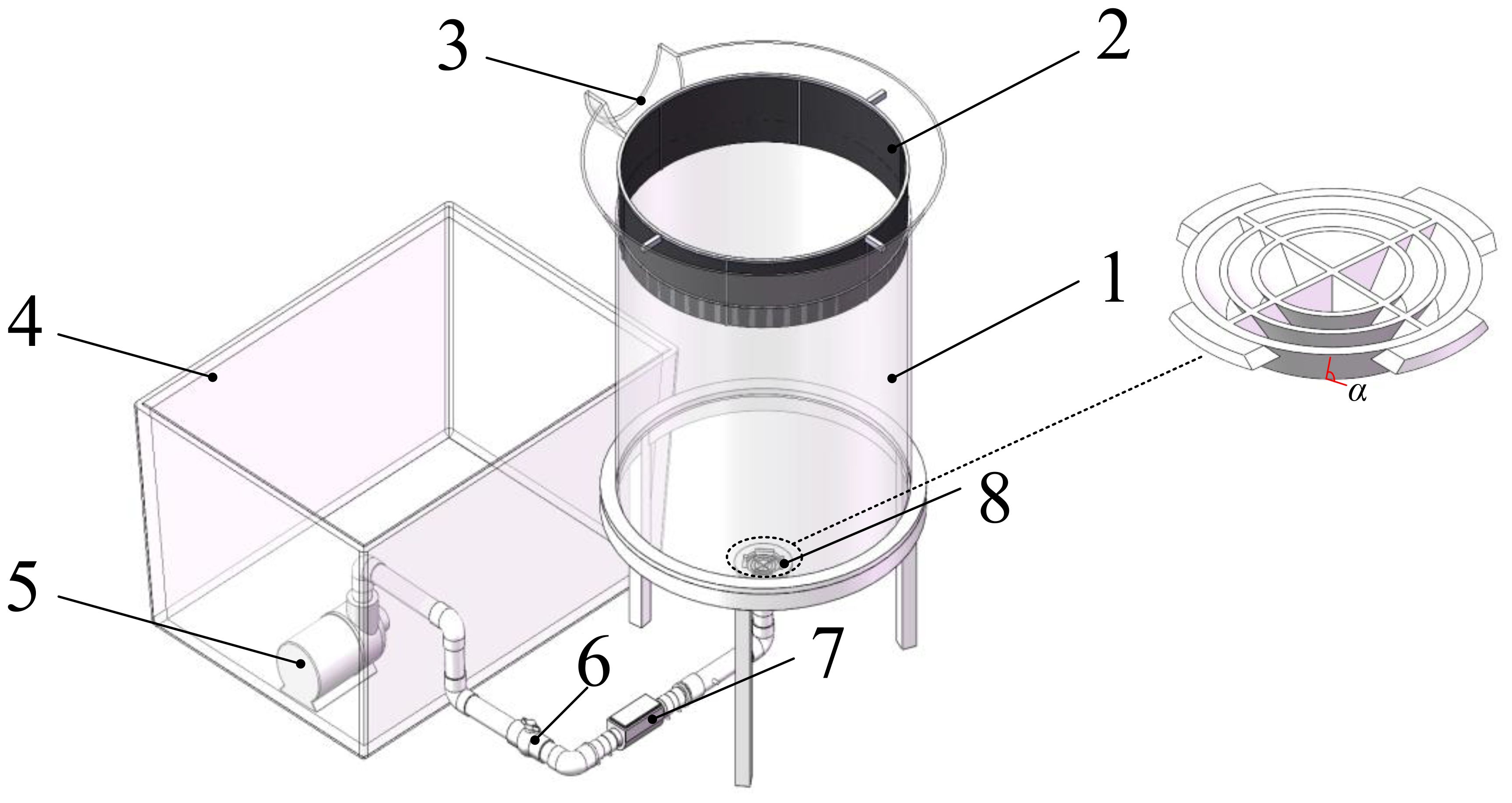
Figure 1 Scallop Larval Cultivation System. 1. culture cone 2. filter screen 3. overflow port 4. reservoir 5. pump 6. ball valve 7. flowmeter 8. deflector.
Building a three-dimensional model of culture cone in Solid works software. The model is scaled to 1:10 in order to increase simulation efficiency. Following the model’s import into Workbench’s Mesh module, the cylindrical and conical meshes are drawn using the O-shaped mesh approach, perform surface treatment and volume mesh treatment, refine the mesh on the inlet and outlet at the same time, the system mesh division is shown in Figure 2.
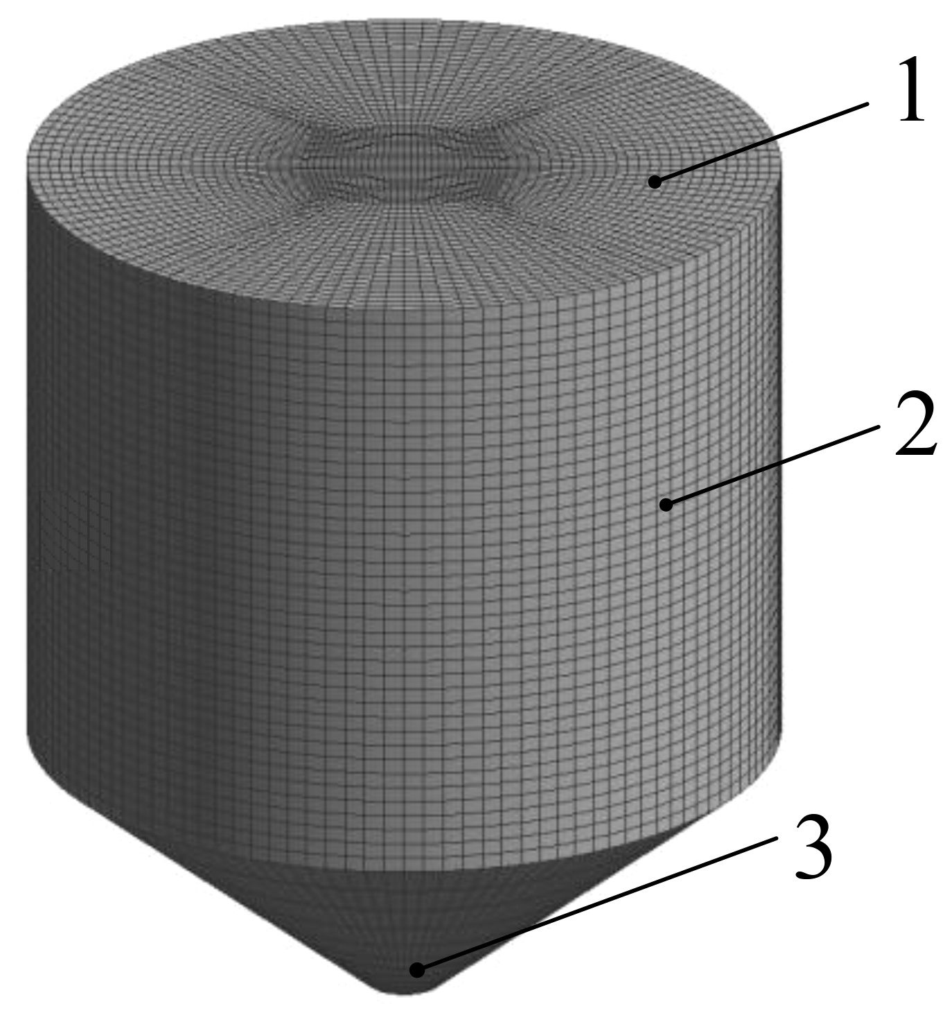
Figure 2 Mesh partitioning schematic. 1.outlet 2. culture cone 3. Inlet.
The accuracy of numerical simulation results depends on the quality of the mesh, and using too many meshes can lengthen the running time. With the same other settings, the coefficient of variation in radial distribution of D-shaped larvae in eight different mesh numbers of culture cone models—49 223 (mesh-1), 100 548 (mesh-2), 151 562 (mesh-3), 201 215 (mesh-4), 250 412 (mesh-5), 300 120 (mesh-6), 351 231 (mesh-7), and 400 275 (mesh-8)—was systematically compared in this study, the results are shown in Figure 3. It can be seen from figure that as the number of meshes reaches 201 215 (mesh-4), the coefficient of variation in radial distribution has minimal variation. Therefore, the subsequent numerical simulation models were all mesh processed according to the mesh-4 standard, with a mesh size of approximately 200 000.
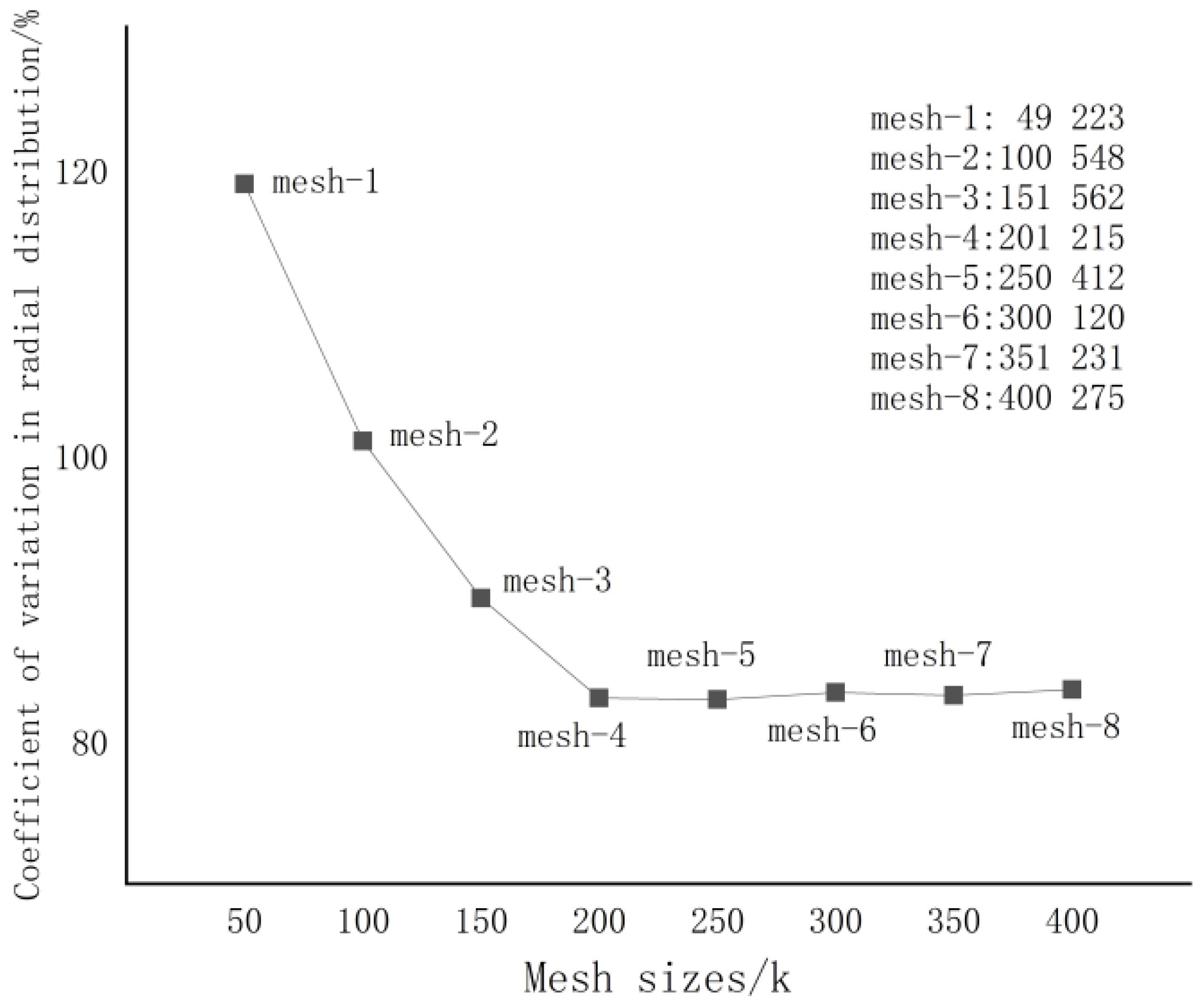
Figure 3 Mesh independence verification results. Conditions: a bottom cone angle(θ) of 90°, a column height/cone height ratio(n) of 2, an inflow velocity(v) of 0.2 m/s, and a simulating time of 40 seconds.
The movement of D-shaped larvae under complex force circumstances inside an upwelling culture cone cannot be accurately simulated by traditional CFD simulation or DEM simulation due to methodological limitations. In EDEM-Fluent coupled simulation, numerical simulation based on discrete element can accurately analyze the mechanical behavior of D-shaped larvae, while numerical simulation based on fluid can accurately describe the fluid mechanical behavior, thus obtaining simulation results that are more in line with the true motion of D-shaped larvae in the culture cone. This paper provides a foundation for culture cone optimization by analyzing the distribution of D-shaped larvae under various cone structures and operating parameters through single factor experiments and orthogonal rotation experiments using EDEM-Fluent coupled simulation.
Select RNG k- ϵ turbulence model as the fluid flow model, compared to using standard k- ϵ models, RNG k- ϵ model has advantages in dealing with flows with high strain rates and significant streamline curvature (Labatut et al., 2015). This model modifies the turbulence viscosity, taking into account the anisotropy of turbulence in practical situations and the rotational flow in mean flow. The generation term in the RNG k-ϵ model is related to flow and spatial location. The above improvements have enabled RNG k- ϵ model compared to standard k- ϵ model yields more accurate results (An et al., 2018; Shi, 2018).
Using RNG k- ϵ model establishment fluid numerical model, turbulent kinetic energy (k) equation and turbulent dissipation rate (ϵ) equation is as shown in Equations 1, 2:
turbulent kinetic energy equation:
turbulent dissipation rate equation:
where t is the time,s; ρ is the fluid density, kg/m3; x is the displacement component,m;u is the velocity vector,m/s; i, j are tensor indices, range (1, 2, 3); μ is the fluid dynamic viscosity, Pa·s; , are reciprocals of the turbulent kinetic k and turbulent dissipation rate ϵ; Gk is the generation term of turbulent kinetic energy due to the mean velocity gradients; , are empirical constants in the model, typically set to =1.44 and =1.92 based on empirical data.
This paper mainly studies the effects of culture cone structure and inflow velocity on the movement of scallop larvae. Among them, the larval particle phase is considered as a discrete phase and the fluid is considered as a continuous phase. By solving the Discrete Phase Model (DPM), the statistics of the particles are obtained. Water is the main body inside the culture cone, and the proportion of larval particles is generally small (<10%). Moreover, larval particles move along their own trajectories, making it suitable to use the Lagrangian method for modeling and calculation. Therefore, in this study, the DPM model was selected for numerical calculation and analysis of solid particles (Chen et al., 2014; Gorle et al., 2018; Dauda et al., 2019).
This method solves particle trajectories by calculating the integral equation of the motion differential equation acting on particles in Lagrange coordinates, the differential equation for the force acting on larval particles is as shown in Equations 3, 4:
where is the particle velocity, m/s; is the particle density, kg/m3; is the drag force experienced by a unit mass particle, N; / is the gravitational force per unit mass acting on the particle, N; is the component of other various forces in the X direction, N.
where is the particle diameter,mm; is the drag coefficient; is the relative Reynolds number of the particle.
The advantage of the EDEM-Fluent coupling method lies in its ability to employ the most suitable simulation methods for both liquids and particles. The interactions between liquids and particles can be accurately depicted through correctly creating the connection between EDEM and Fluent. The time step, along with the material properties of particles and liquids, are adjusted based on the actual situation.
Both Fluent and EDEM have their own time steps, which must match when they are coupled. Since the particle phase’s time step is only 10%–30% of the Rayleigh time step, which is significantly less than Fluent’s time step, neither phase’s time steps need to be adjusted to 1:1. The time step in Fluent is typically significantly bigger than that in EDEM in order to accurately capture the contact behavior between particles in coupling, and the ratio of EDEM time step to Fluent time step is frequently set between 1:10 and 1:100.
Three requirements need to be met for the coupling to be successful, as verified by testing:
● Fluent’s time step ought to guarantee the convergence of fluid computations;
● The time step in EDEM cannot be larger than the time step in Fluent and must adhere to the Rayleigh time step setting standards;
● Both the intervals used for data storage and the temporal step size in Fluent should be integer multiples of those in EDEM.
The simulation solving configuration and boundary conditions in Fluent:
● For the whole watershed, the initial relative pressure value is 0pa;
● The boundary of the inlet adopts a velocity inlet, and the inlet velocity is determined by different experiments;
● The outlet boundary adopts a pressure outlet, with an initial relative pressure value of 0pa;
● The outer wall of the computational domain is a no-slip wall surface, and there is no heat transfer throughout the simulation, so the energy equation is not calculated.
The simulation solving configuration and boundary conditions in EDEM: This article’s particle simulations don’t include complicated scenarios like fragmentation and deformation, and their particle mass load is less than 0.01%. It is therefore sufficient to take into account solely particle collisions and particle collisions with walls. For both particle-particle and particle-wall contact models in the simulation, the fundamental Hertz-Mindlin model can be applied. The Wen&Yu drag force model is employed for the drag force calculation. The Rayleigh time step of 0.1mm particle size in this article is 5.67 × 10⁻⁷ s. The EDEM time step is set at 17.64% of the Rayleigh time step, is 1.0 × 10⁻⁷ s, and the Fluent time step is set to 1.0 × 10⁻⁵ s. The three conditions for a successful coupling are satisfied by the time step ratio, which is set to 1:100. Testing reveals that the convergence is good. The remaining particulars parameters are shown in Table 1.
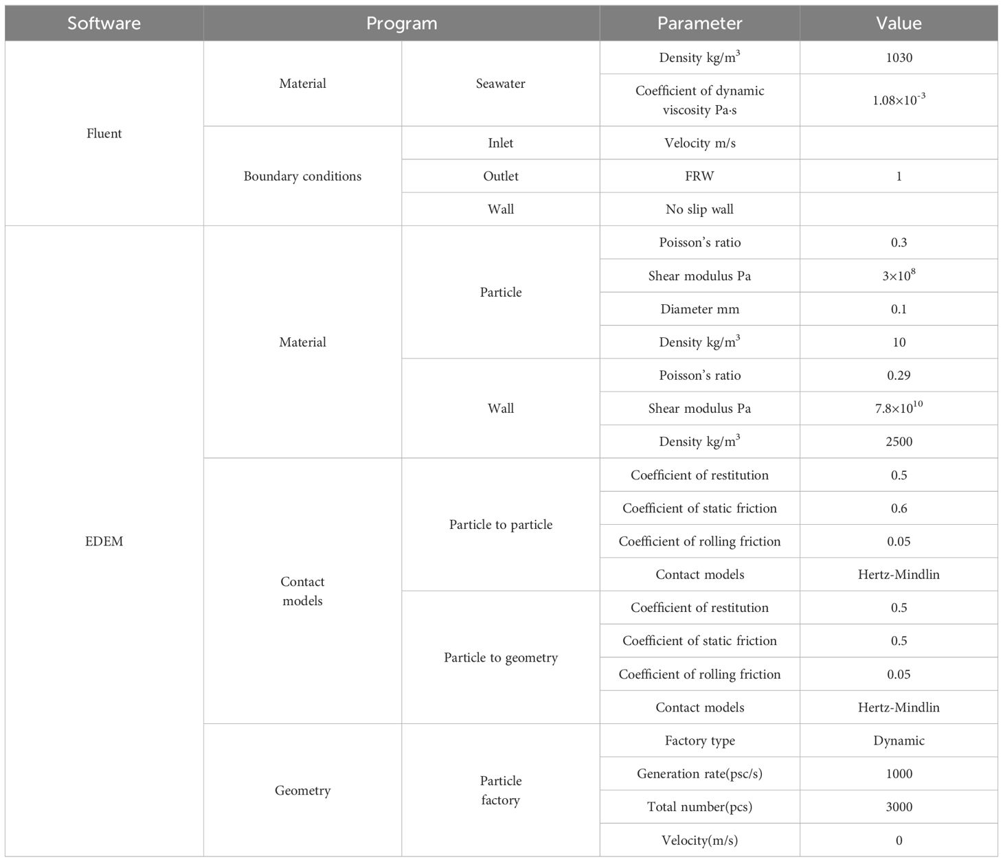
Table 1 Numerical computation parameter.
Perform the following steps to establish coupling between EDEM and Fluent:
● Open the tool window in EDEM related to the coupling interface;
● Select “Start” to put EDEM in a state where it listens for coupling signals and awaits connection with Fluent;
● In Fluent, import the “loadedemcoupling.jou” file;
● In the EDEM Coupling model within Fluent, check the “Use DDPM” option;
● Proceed to establish the connection
The coefficient of variation of the scallop larval distribution was employed as an evaluation index to investigate the uniformity of the distribution of scallop larvae in the culture cone. The Equation 5 is used to compute the radial distribution coefficient of variation and the axial distribution coefficient of variation of scallop larvae. Note that the number of scallop larvae in the k (1–10) annular region depicted in Figure 4A is represented by the value of mk when computing the radial distribution coefficient of variation; The number of scallop larvae in the k (1–10) columnar region depicted in Figure 4B is denoted by the value of mk when calculating the coefficient of variation of axial distribution, each region’s cultured water is 10L.
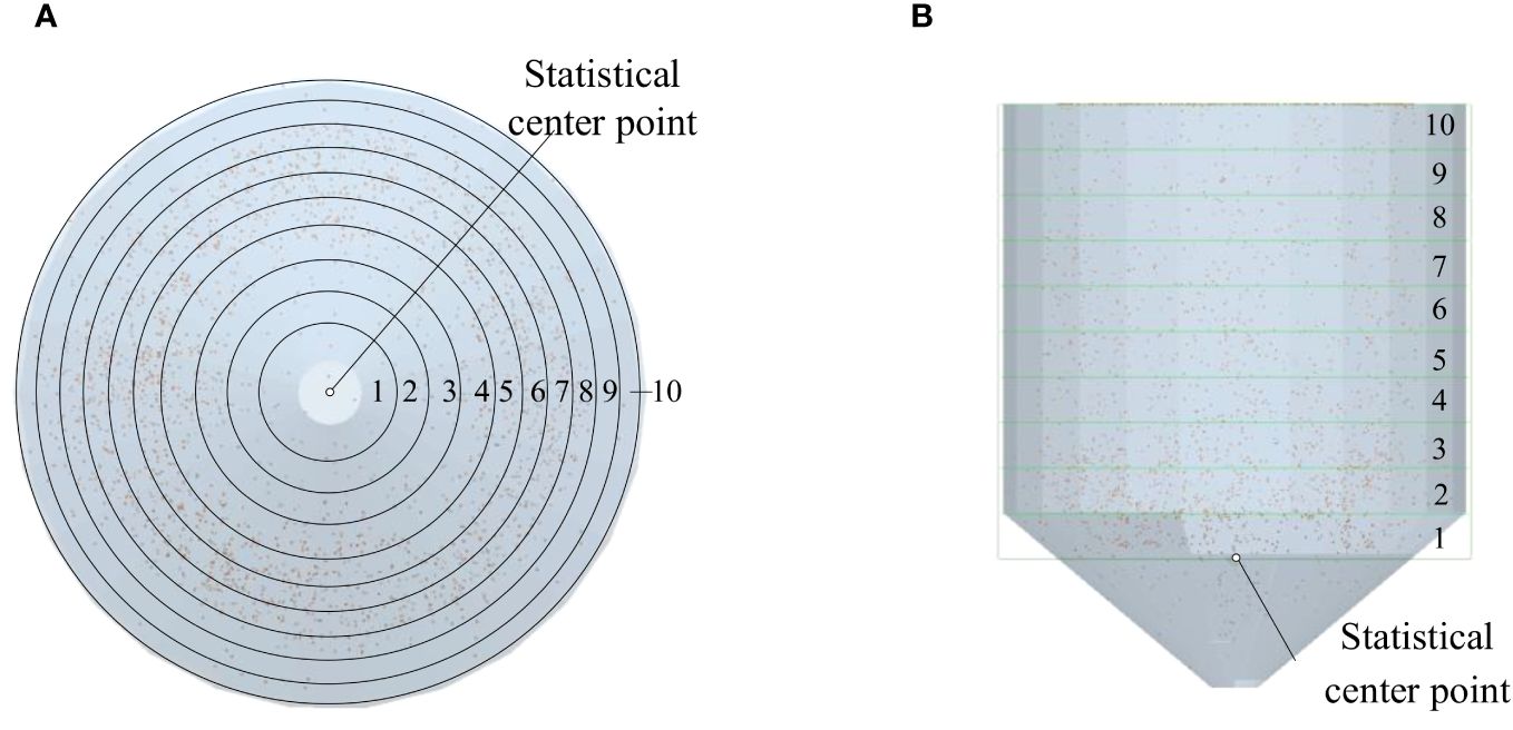
Figure 4 Schematic Diagram of Statistical Area Division (A) Radial; (B) Axial.
In order to examine the impact of the bottom cone angle (θ), the column height/cone height ratio(n), and the inflow velocity(v)on the distribution of scallop larvae within the culture cone, a single factor simulation experiment was initially conducted. In this experiment, change the value of the individual factor to be examined, while the remaining factors remain unchanged at the midpoint of their respective value ranges. The distance from the statistical center point to the single-column statistical region with the highest abundance of scallop larvae is defined as the distance of peak value, with the quantity of scallop larvae in that region being denoted as the peak value of the scallop larvae distribution.
Referring to the cone angle design of existing conical incubators, Zhang Renming used a conical incubator with a bottom cone angle of 56° for fish egg hatching, Rico Villa (Rico-Villa et al., 2008) used a bottom cone angle of 87° for the study of the Pacific oyster juvenile flow cultivation system, and Mi Guoqiang used a suspended aeration incubator with a bottom cone angle of 137° for fish egg hatching. The variation range of the bottom cone angle (θ) in this experiment is 60°~140°, with an increment of 20°. The inflow velocity (v) is 0.25m/s, and the column height/cone height ratio (n) is 2,the distribution of scallop larvae is shown in Figure 5. The scallop larvae’s radial distribution is shown in Figure 5A. The peak value of the scallop larvae distribution first declines and then increases as the bottom cone angle(θ) rises, while the coefficient of variation first decreases and then increases; According to Figure 5B, it can be seen that the axial distribution of scallop larvae, the peak value of the scallop larvae distribution appears at both ends of the statistical area. The coefficient of variation initially falls and then increases as the bottom cone angle(θ) rises, while the peak value of the scallop larvae distribution first decreases and then grows. The radial and axial coefficient of variation is minimum at the bottom cone angle(θ) of 100°. According to the analysis, if the culture cone’s bottom cone angle(θ) is too big or too small, the scallop larvae will concentrate in a particular area along the radial or axial direction of the cone, which isn’t good for the larvae’s uniform spatial distribution.
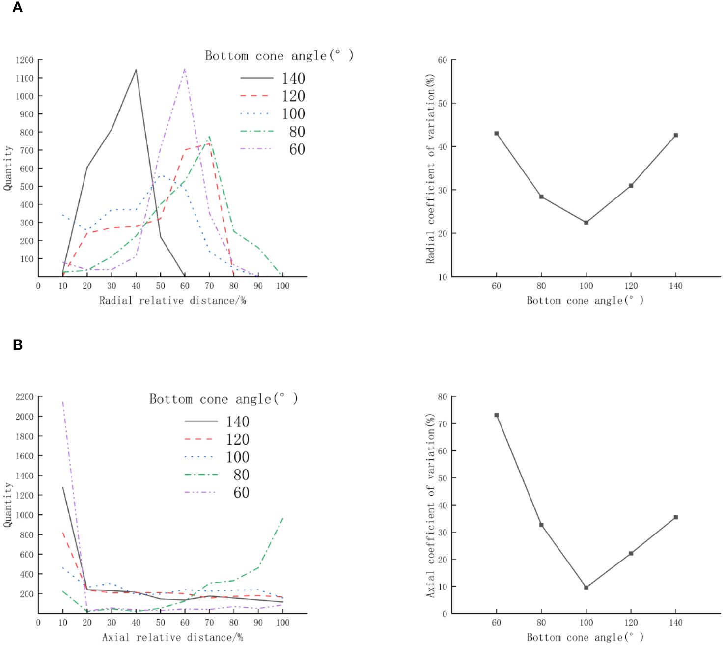
Figure 5 Effect of bottom cone angle (θ) on the distribution of D-shaped larvae (A) Radial; (B) Axial.
Referring to the column height/cone height ratio design of existing conical incubators, Zhang Renming used a conical incubator with a column height/cone height ratio of 0.8 for fish egg hatching, Mi Guoqiang used a suspended aeration incubator with a column height/cone height ratio of 1.6 for fish egg hatching, and Rico Villa used a column height/cone height ratio of 2.7 for the study of Pacific oyster juvenile flow cultivation systems. The variation range of the column height/cone height ratio (n) in this experiment is 1-3, with an increment of 0.5. The inflow velocity (v) is 0.25m/s, and the bottom cone angle (θ) is 100° the distribution of scallop larvae is shown in Figure 6. According to Figure 6A, it can be seen that the radial distribution of scallop larvae, as the column height/cone height ratio(n) increases, the distance of peak value changes slightly and reaching minimum when the column height/cone height ratio(n) is 3, the peak value of the scallop larvae distribution is close, and the coefficient of variation first decreases and then increases. According to Figure 5B, it can be seen that the axial distribution of scallop larvae, the peak value of the scallop larvae distribution occurs at both ends of the statistical area. As the column height/cone height ratio(n) increases, the peak value of the scallop larvae distribution first decreases and then increases, and the coefficient of variation first decreases and then increases. The minimal coefficient of variation is concurrently reached when the column height/cone height ratio (n) is 2. This is because an excessively large or small column height/cone height ratio(n) might result in scallop larvae being concentrated at the top or bottom of the culture cone, with notable variations in the scallop larvae’s axial distribution.
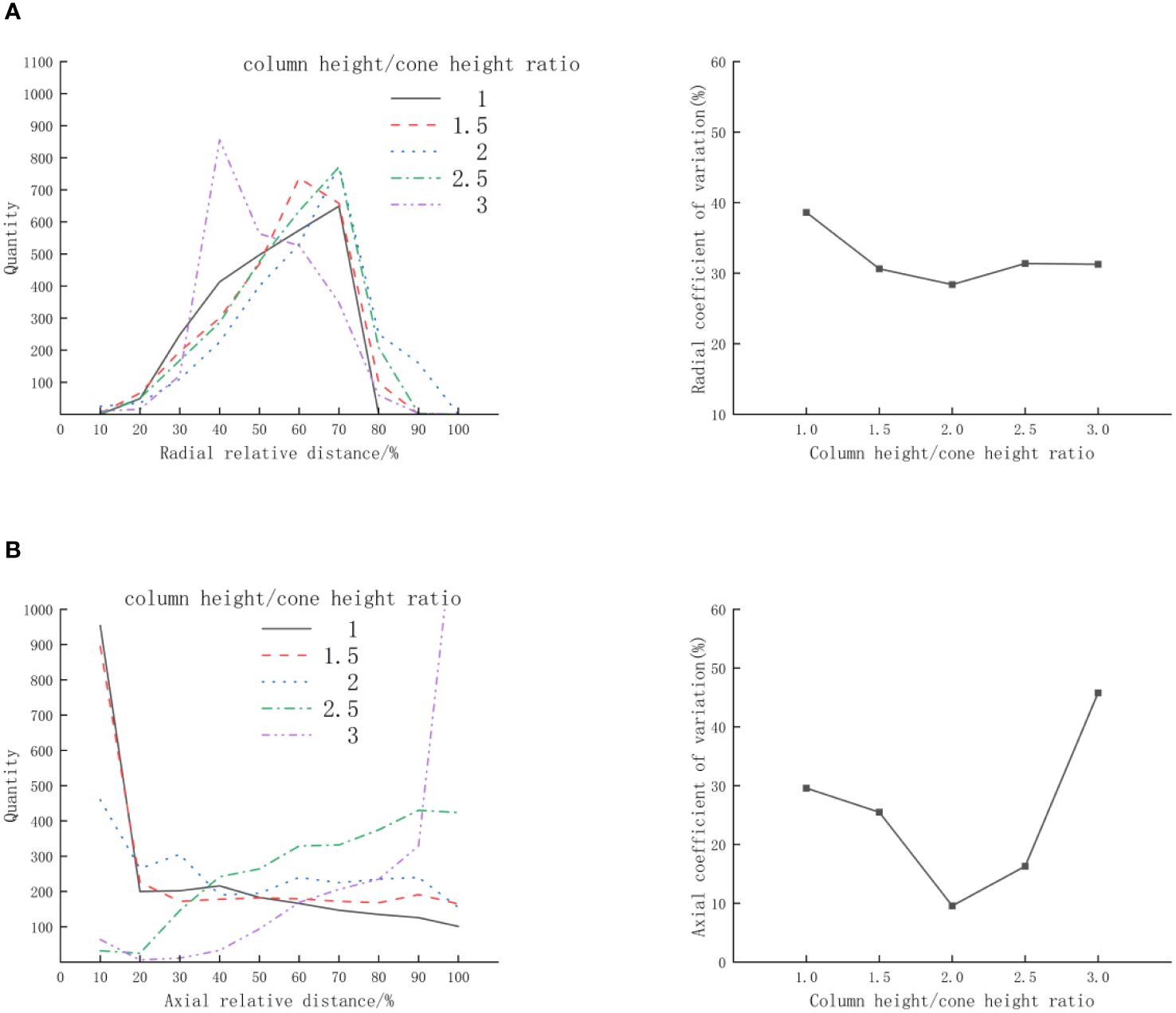
Figure 6 Effect of column height/cone height ratio (n)on the distribution of D-shaped larvae (A) Radial; (B) Axial.
A bottom cone angle(θ) of 100°, a column height/cone height ratio(n)of 2, based on the water flow velocity in natural sea areas for scallop larvae, the variation range of inflow velocity(v) is selected as 0.15~0.35 m/s, with an increment of 0.05 m/s, the distribution of scallop larvae is shown in Figure 7. It is evident from Figure 7A that as inflow velocity(v) rise, the distance of peak value rise, the peak value of the scallop larvae distribution first increases and then decreases, the coefficient of variation is not significantly different. According to Figure 7B, it can be seen that the axial distribution of scallop larvae, the peak value of the scallop larvae distribution appears at both ends of the statistical area. As the inflow velocity(v) increases, the peak value of the scallop larvae distribution first decreases and then increases, and the coefficient of variation first decreases and then increases. This is because scallop larvae may concentrate at the top or bottom of the culture cone due to an excessively high or low inflow velocity(v). The axial distribution of scallop larvae exhibits considerable differences, even in cases when the radial distribution uniformity is not significantly different.
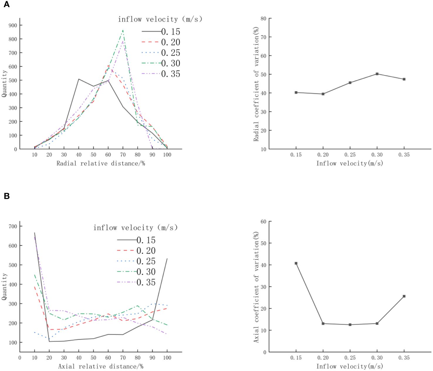
Figure 7 Effect of inflow velocity(v) on the distribution of D-shaped larvae (A) Radial; (B) Axial.
Based on the aforementioned single-factor experiments, the levels of each factor were determined, and conducting three-factor three-level rotational orthogonal combination experimental (Ren, 2009; Xu and He, 2010). The experimental arm length(γ) was set to 1, and the encoding for each level is presented in Table 2. The experimental design and results are outlined in Table 3.
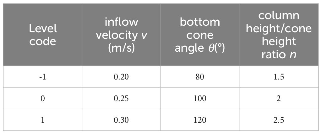
Table 2 Factor level coding table.
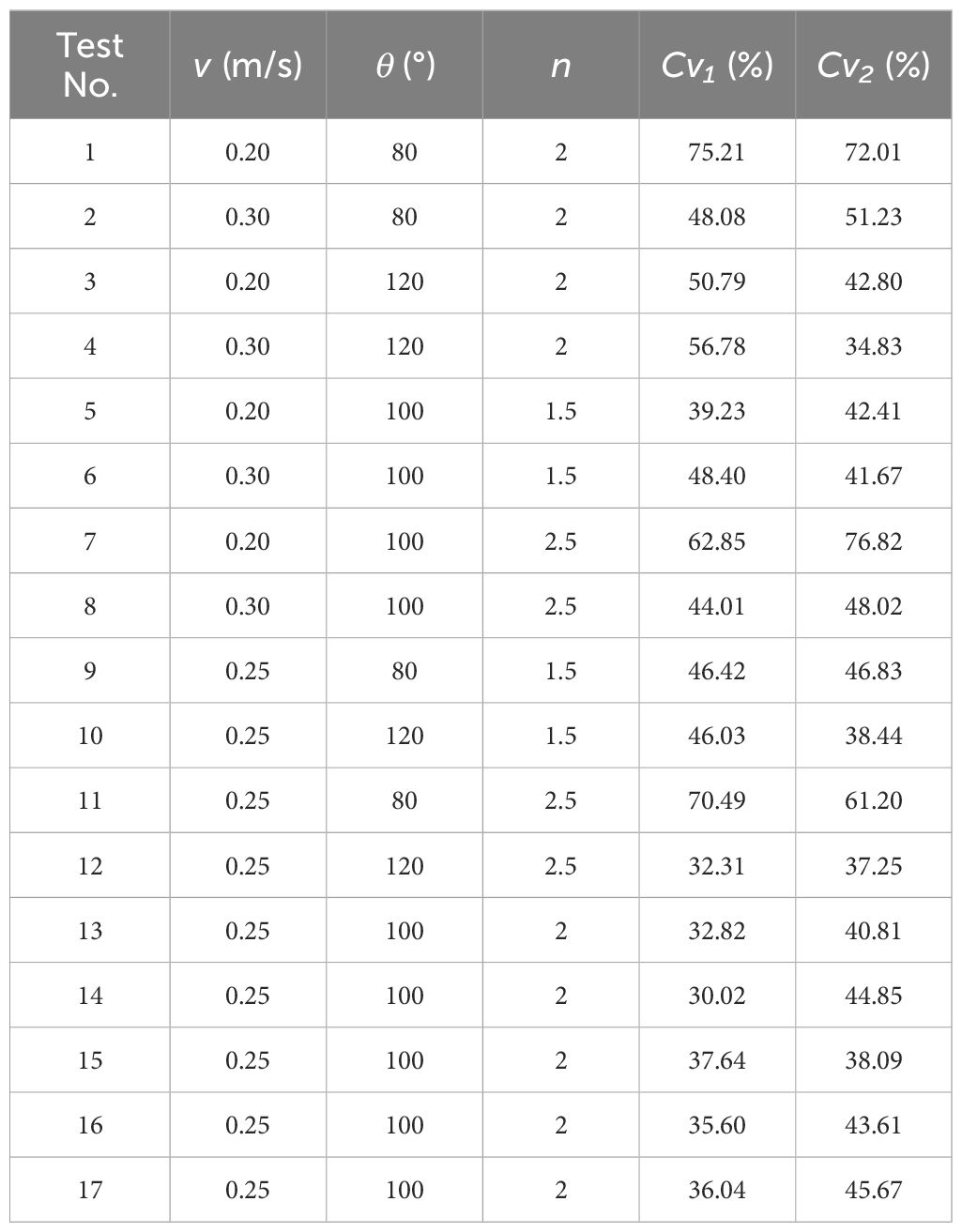
Table 3 Test scheme and results.
The experimental results in the table were subjected to multivariate regression analysis using Design-Expert software. Subsequently, factors with insignificant effects on the experimental indicators were gradually removed. The analysis of variance is shown in Tables 4, 5, the lack-of-fit is not significant.
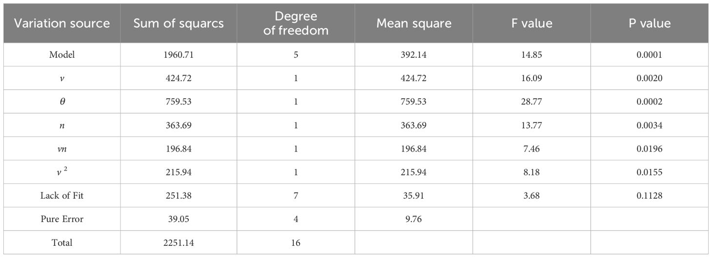
Table 4 ANOVA of the radial coefficient of variation of D-shaped larval distribution.
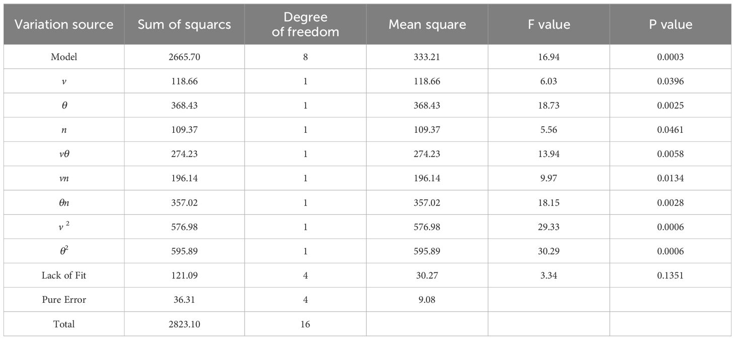
Table 5 ANOVA of the axial coefficient of variation of D-shaped larval distribution.
Regression analysis was conducted on the simulated experimental results of the radial distribution coefficient response surface for scallop larvae, yielding the following quadratic regression model:
where is the radial distribution coefficient of scallop larvae, %; v is the inflow velocity, m/s; θ is the bottom cone angle, °; n is the column height/cone height ratio.
From Table 4, The regression model shown in Equation 6 is used to describe the relationship between the radial distribution coefficient of variation of scallop larvae and various factors, the P-value (0.0001) which is significantly less than 0.01, indicates that the regression model is highly significant. Furthermore, the P-values corresponding to the bottom cone angle(θ), inflow velocity(v), and column height/cone height ratio (n) are all less than 0.01, indicating that both aforementioned factors have a highly significant impact on the radial distribution coefficient of scallop larvae. The order of influence of these three factors, as determined by the magnitude of the P-values, is as follows: bottom cone angle(θ)>inflow velocity(v)> column height/cone height ratio(n). Furthermore, the interaction term between inflow velocity(v) and column height/cone height ratio(n) (P=0.0196), as well as the square term of inflow velocity(v) (P=0.0155), have significant effects on the radial distribution coefficient. The interactions and square terms of the remaining factors are not significant.
Regression analysis was conducted on the simulated experimental results of the axial distribution coefficient response surface for scallop larvae, yielding the following quadratic regression model:
From Table 5, it can be observed that the regression model described by Equation 7 depicts the relationship between the coefficient of variation in axial distribution of scallop larvae and the various factors. The P-value (0.0003) is much smaller than 0.01, indicating that the regression model is highly significant. Furthermore, the corresponding P-values for the bottom cone angle(θ) are less than 0.01, indicating its highly significant impact on the axial distribution coefficient of variation. The inflow velocity(v)and column height/cone height ratio(n) have P-values less than 0.05, signifying a significant influence on the radial distribution coefficient of variation of scallop larvae. In terms of the magnitude of P-values, the order of influence of these three factors is bottom cone angle(θ)>inflow velocity(v)> column height/cone height ratio(n). Additionally, the P-values for the interaction terms between any two factors among the three [inflow velocity(v) × bottom cone angle(θ), inflow velocity (v)× column height/cone height ratio(n), bottom cone angle(θ) × column height/cone height ratio(n)] are all less than 0.05, indicating significant effects of these interactions on the axial distribution coefficient of variation. Furthermore, the square terms of inflow velocity(v) and bottom cone angle(θ) (P<0.01) also exhibit highly significant effects on the axial distribution coefficient of variation.
Response surface analysis was performed on the significant interaction terms identified in the analysis of variance table using Design Expert software, as illustrated in Figure 8.
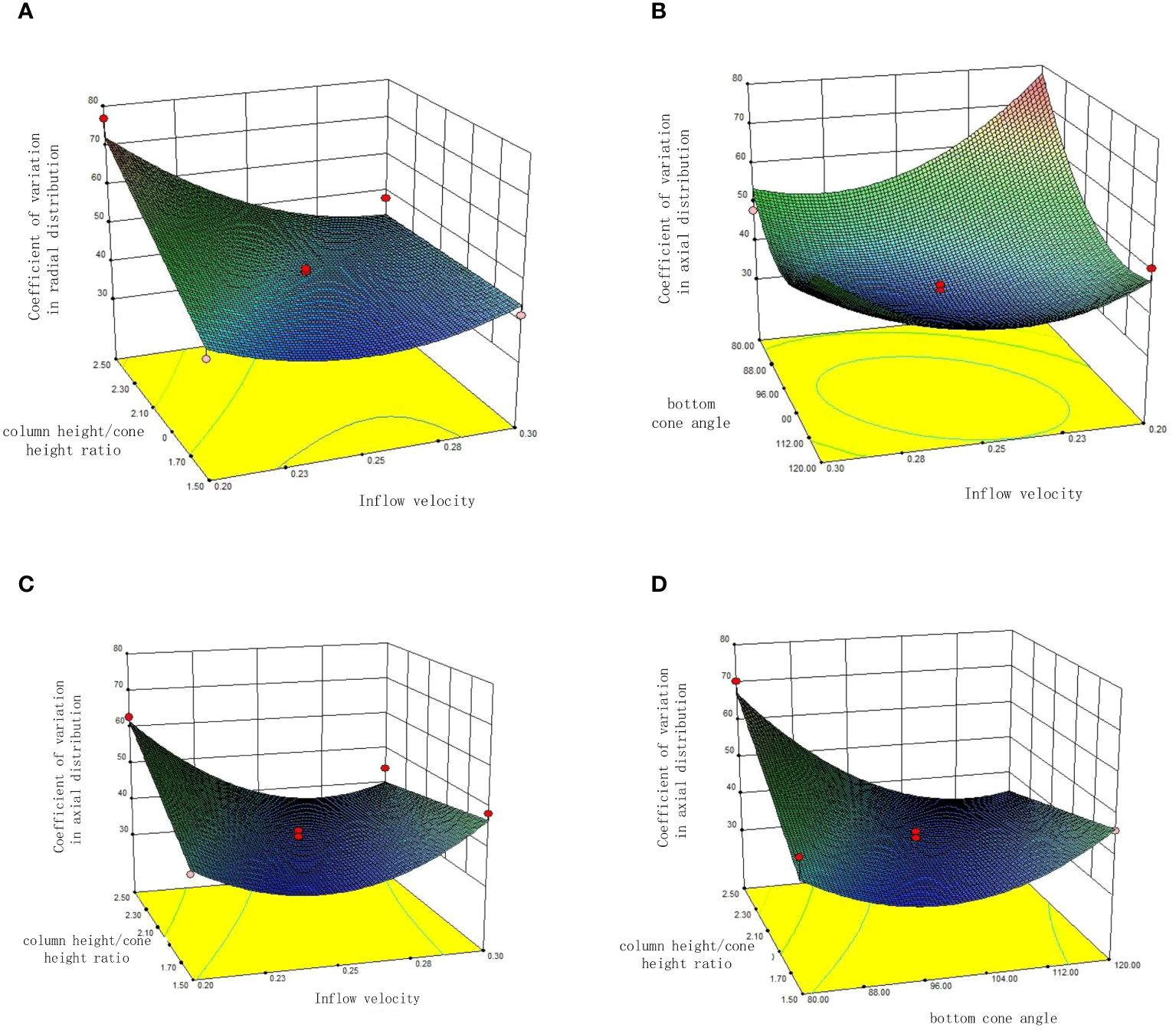
Figure 8 Response surface diagram (A) Interaction of inflow velocity(v) and column height/cone height ratio(n) on coefficient of variation in radial distribution; (B) Interaction of inflow velocity (v) and bottom cone angle (θ) on coefficient of variation in axial distribution; (C) Interaction of inflow velocity(v) and column height/cone height ratio(n) on coefficient of variation in axial distribution; (D) Interaction of angle of the bottom cone(θ) and column height/cone height ratio(n) on coefficient of variation in axial distribution.
At a bottom cone angle(θ) of 100°, the response surface of inflow velocity (v) and column height/cone height ratio (n)on the coefficient of variation in radial distribution of scallop larvae is depicted in Figure 8A. At a constant inflow velocity(v), the coefficient of variation in radial distribution is directly proportional to the column height/cone height ratio(n). Moreover, as the inflow velocity(v) increases, the influence of the column height/cone height ratio (n) on the radial variation coefficient diminishes. When the inflow velocity (v) reaches 0.3 m/s, the effect of the column height/cone height ratio(n) on the radial distribution variation coefficient becomes negligible. When the column height/cone height ratio(n) exceeds 2, the radial variation coefficient is inversely proportional to the inflow velocity(v). When the column height/cone height ratio(n) is less than 2, as the flow velocity(v) increases, the radial coefficient of variation first decreases and then increases, and as the column height/cone height ratio (n)decreases, the flow velocity(v) corresponding to the minimum radial coefficient of variation also decreases.
At a column height/cone height ratio(n) of 2, the response surface of inflow velocity(v) and bottom cone angle (θ) on the coefficient of variation in axial distribution of scallop larvae is depicted in Figure 8B. With constant inflow velocity(v), the coefficient of variation in axial distribution initially decreases and then increases with increasing bottom cone angle(θ). Similarly, with constant bottom cone angle(θ), the coefficient of variation in axial distribution initially decreases and then increases with increasing inflow velocity(v).
At a bottom cone angle (θ) of 100°, the response surface of inflow velocity (v) and column height/cone height ratio(θ) on the coefficient of variation in axial distribution of scallop larvae is depicted in Figure 8C. With a constant column height/cone height ratio(n), the coefficient of variation in axial distribution initially decreases and then increases with increasing inflow velocity(v). Additionally, with an increasing column height/cone height ratio(n), the flow velocity corresponding to the lowest axial coefficient of variation(v) increases. When the inflow velocity(v) is less than 0.3 m/s, the axial variation coefficient is directly proportional to the column height/cone height ratio(n), whereas the inflow velocity(v) exceeds 0.3 m/s, the axial variation coefficient is inversely proportional to the column height/cone height ratio(n).
At an inflow velocity(v) of 0.25 m/s, the response surface of bottom cone angle(θ) and column height/cone height ratio (n)on the coefficient of variation in axial distribution of scallop larvae is illustrated in Figure 8D. With a constant column height/cone height ratio(n), the coefficient of variation in axial distribution initially decreases and then increases with increasing bottom cone angle(θ). When the bottom cone angle(θ) is less than 110°, the axial variation coefficient is directly proportional to the column height/cone height ratio(n), whereas when the bottom cone angle(θ) exceeds 110°, the axial variation coefficient is inversely proportional to the column height/cone height ratio(n).
The structural parameters such as cone angle (θ) and column height/cone height ratio (n) have a significant impact on the spatial distribution of D-shaped larvae in the culture cone. In order to improve the uniformity of the spatial distribution of D-shaped larvae in the culture cone, the optimization objective is to minimize the radial and axial distribution variation coefficients of D-shaped larvae. The inflow velocity is limited to 0.20 m/s~0.30 m/s, the bottom cone angle is limited to 80°~120°, and the column height/cone height ratio is limited to 1.5~2.5. The regression model is solved to obtain the optimal parameter combination, and the relevant constraints are shown in the Equation 8.
The optimal combination function in Design Expert was used to solve the regression model. When the inflow velocity was 0.25m/s, the bottom cone angle cone was 108.97°, and the column height/cone height ratio was 1.8, the experimental factor parameter combination was the best, the radial distribution variation coefficient of D-shaped larvae was 37.21%, and the axial distribution variation coefficient was 36.43%. This parameter combination was applied to Fluent-EDEM coupled simulation verification, and the radial distribution variation coefficient of D-shaped larvae was 38.92%, and the axial distribution variation coefficient was 35.17%. The calculation errors with Design-Expert software were 4.6% and 3.5%, respectively.
To validate the operational performance of the designed culture cone, an experimental prototype was constructed for performance testing, the experimental setup is depicted in Figure 9. Experimental Procedure: A solid model with a bottom cone angle(θ) of 108.97° and a column height/cone height ratio (n) of 1.8:1 was utilized. The flow rate was controlled through a water inlet valve, and D-shaped larvae were introduced into the system. After allowing approximately 10 minutes for water stabilization, high-definition cameras positioned directly above and in front of the culture cone were activated to capture images and record the distribution of the scallop larvae. The imaging was conducted during nighttime using LED light strips for illumination, as illustrated in Figures 10A, B. The captured images were processed using Image J software, including format conversion and grayscale transformation, as depicted in Figure 11, the particle counting method within the software analysis module was employed to quantify the number of scallop larvae within the images. Subsequently, statistical methods can be found in section 3.3, the coefficient of variation was computed using Equation 5.
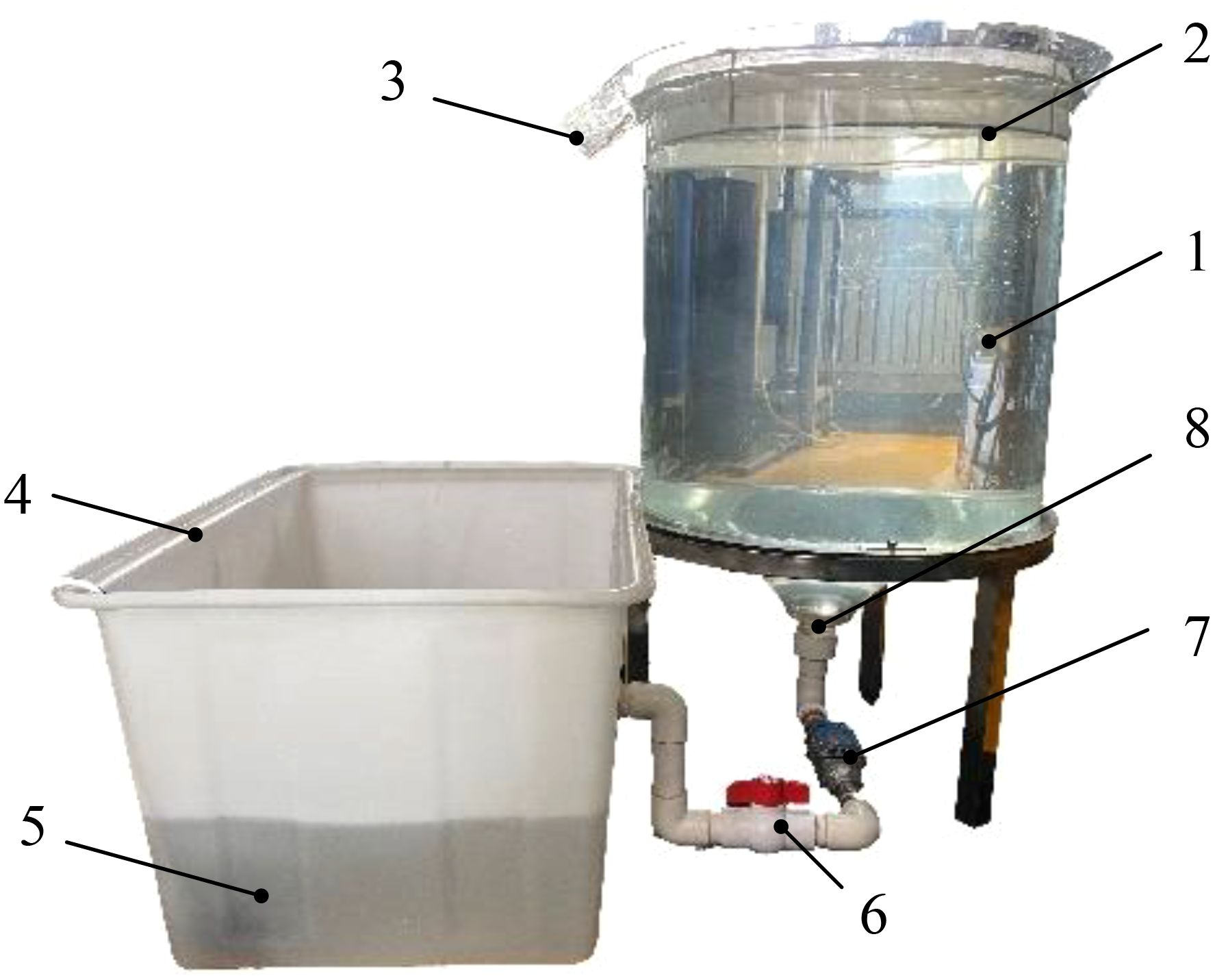
Figure 9 Prototype for testing. 1. culture cone 2. filter screen 3. overflow port 4. reservoir 5. pump 6. ball valve 7. flowmeter 8. Deflector.
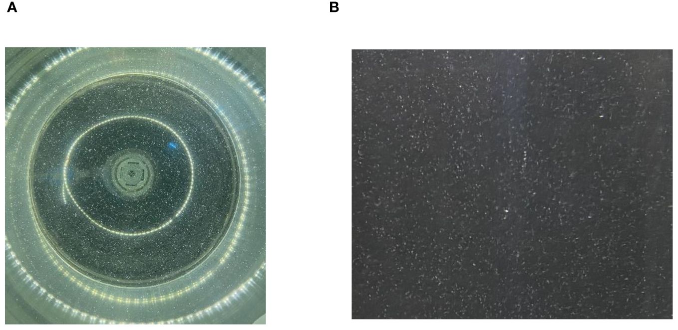
Figure 10 Distribution map of D-shaped larvae. (A) Axial direction; (B) Radial direction.
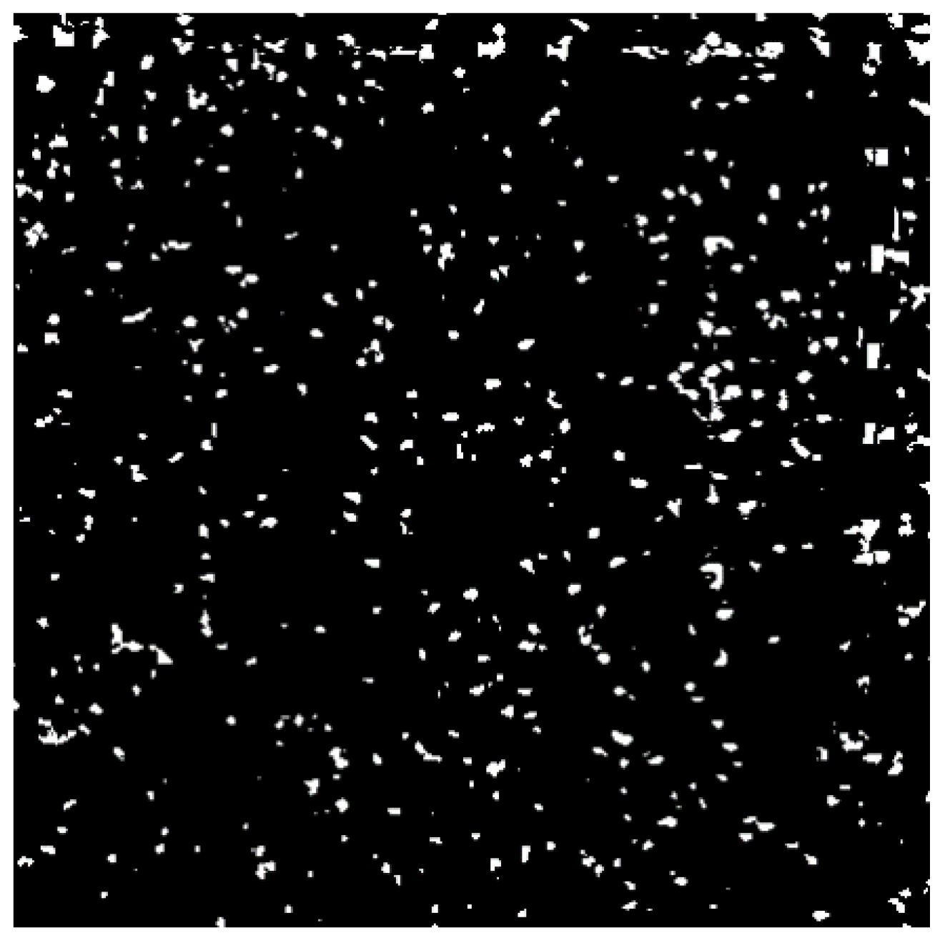
Figure 11 Image processed by Image J.
To investigate the actual effects of different inflow structures on the distribution of D-shaped larvae under identical operational parameters, a three-factor, three-level orthogonal rotation experiment was conducted, with the inlet deflector angle (α), inflow velocity (v), and cultivation density (τ) as factors, with the radial distribution coefficient of variation and axial distribution coefficient of variation as measurement indicators. The experimental factors and their levels are presented in Table 6. The experimental design and results are summarized in Table 7.

Table 6 Factor level coding table.
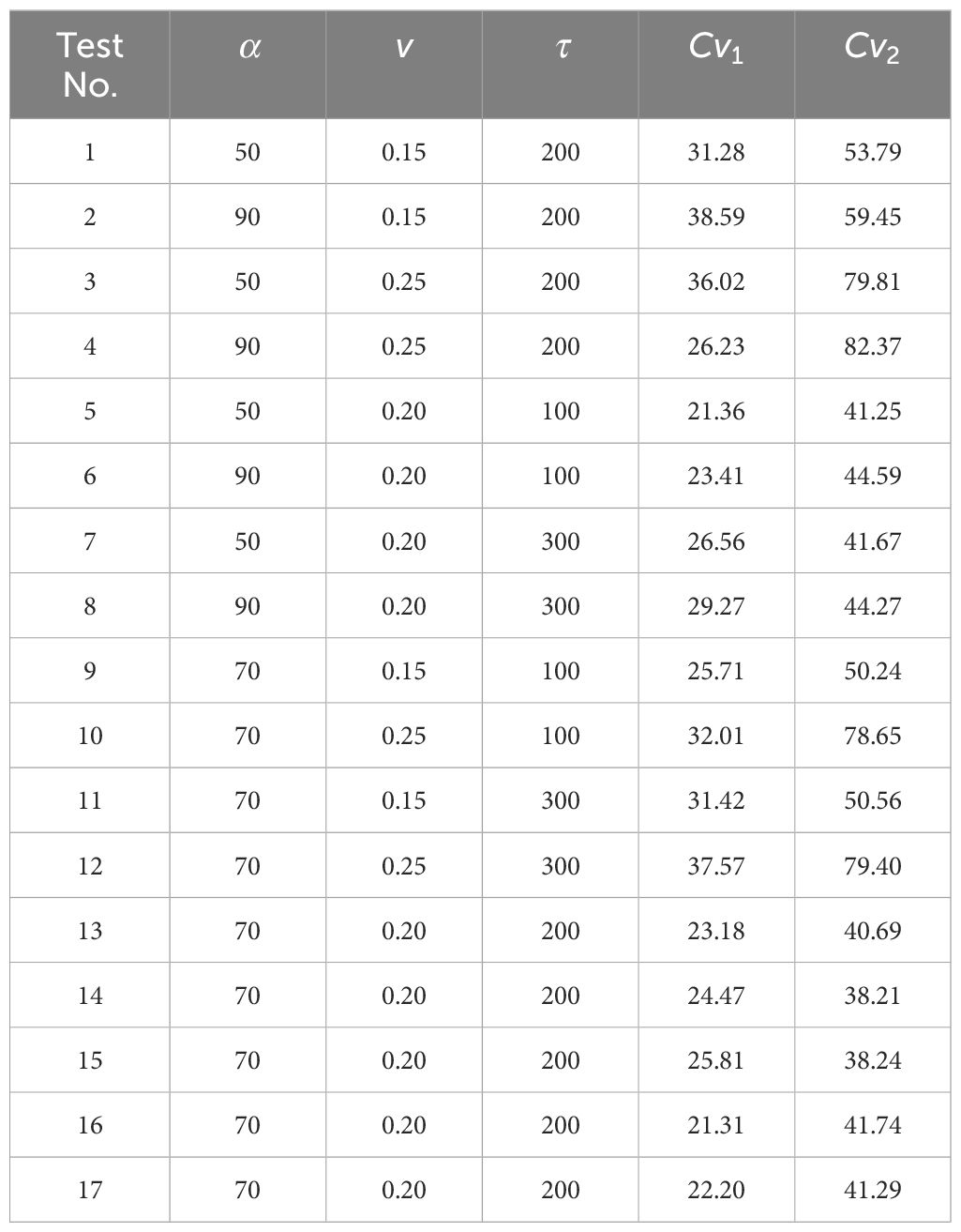
Table 7 Test scheme and results.
The experimental results were subjected to regression analysis using Design Expert software, successively eliminating non-significant terms related to the evaluation criteria. The analysis of variance results are shown in Tables 8, 9.
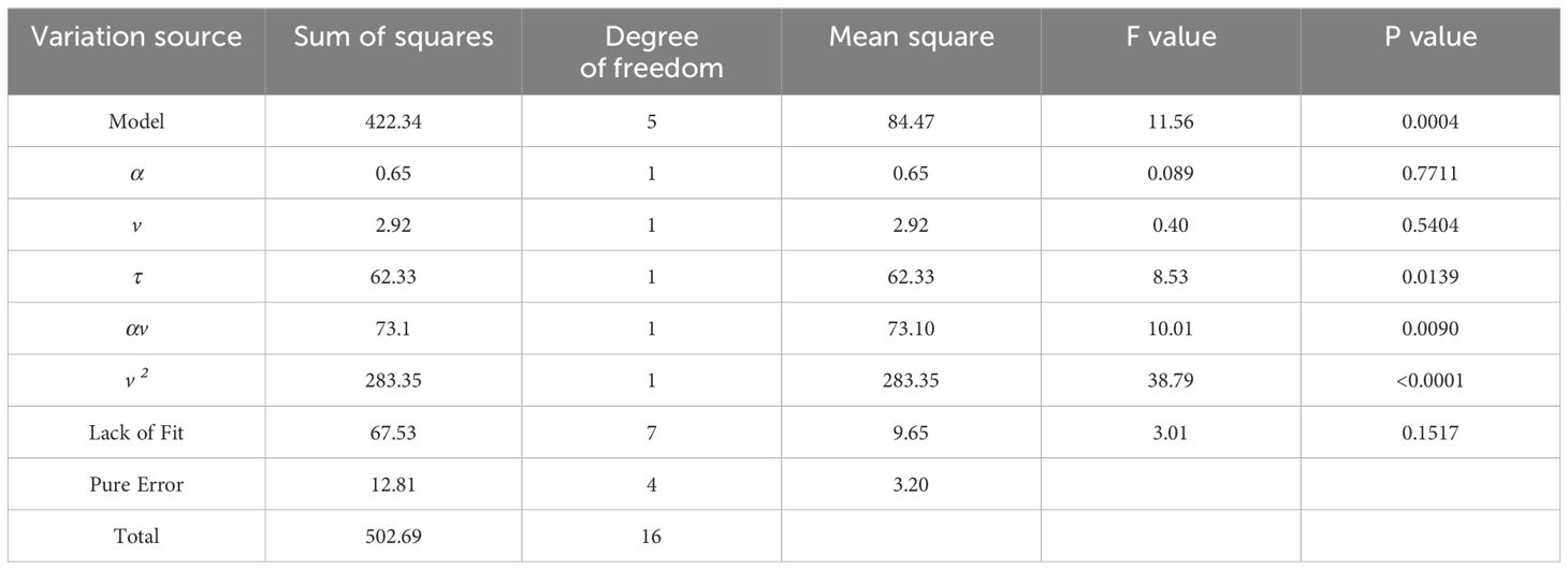
Table 8 ANOVA of the radial coefficient of variation of D-shaped larval distribution.
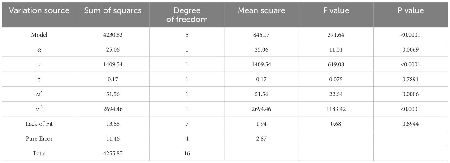
Table 9 ANOVA of the axial coefficient of variation of D-shaped larval distribution.
The analysis results in the table show that the lack-of-fit term in the variance analysis of the radial variation coefficient of D-shaped larvae distribution uniformity is 0.1517, which is greater than 0.05, demonstrating non-significance, indicating that the model can better reflect the influence of various influencing factors on the radial distribution variation coefficient. The inlet deflector angle(α), inflow velocity(v), the interaction term between the inlet deflector angle(α) and inflow velocity(v), and the quadratic term of inflow velocity(v) significantly affect the radial coefficient of variation of D-shaped larval distribution uniformity. The regression equation for the radial coefficient of variation () of D-shaped larval distribution uniformity with respect to each influencing factor is as shown in Equation 9:
The analysis results from the table indicate that the lack-of-fit term for the variance analysis of the axial coefficient of variation of D-shaped larval distribution is 0.6944, which is greater than 0.05, demonstrating non-significance, prove that the model can better reflect the influence of various influencing factors on the coefficient of variation of axial distribution. The inlet deflector angle(α), inflow velocity(v), the quadratic term of the inlet deflector angle(α), and the quadratic term of inflow velocity (v) significantly influence the axial coefficient of variation of D-shaped larval distribution uniformity. The regression equation for the axial coefficient of variation () of D-shaped larval distribution uniformity with each influencing factor is as shown in Equation 10:
When the cultivation density (τ) remains constant, the response surface of the radial coefficient of variation of D-shaped larvae to the inlet deflector angle (α) and inflow velocity(v) is shown in Figure 12. When the flow velocity(v) is less than 0.21 m/s, the radial coefficient of variation is directly proportional to the inlet deflector angle(α); however, when the inflow velocity(v) exceeds 0.21 m/s, the radial coefficient of variation is inversely proportional to the inlet deflector angle(α). Furthermore, when the inlet deflector angle(α) is constant, the radial coefficient of variation decreases initially and then increases with increasing inflow velocity(v).
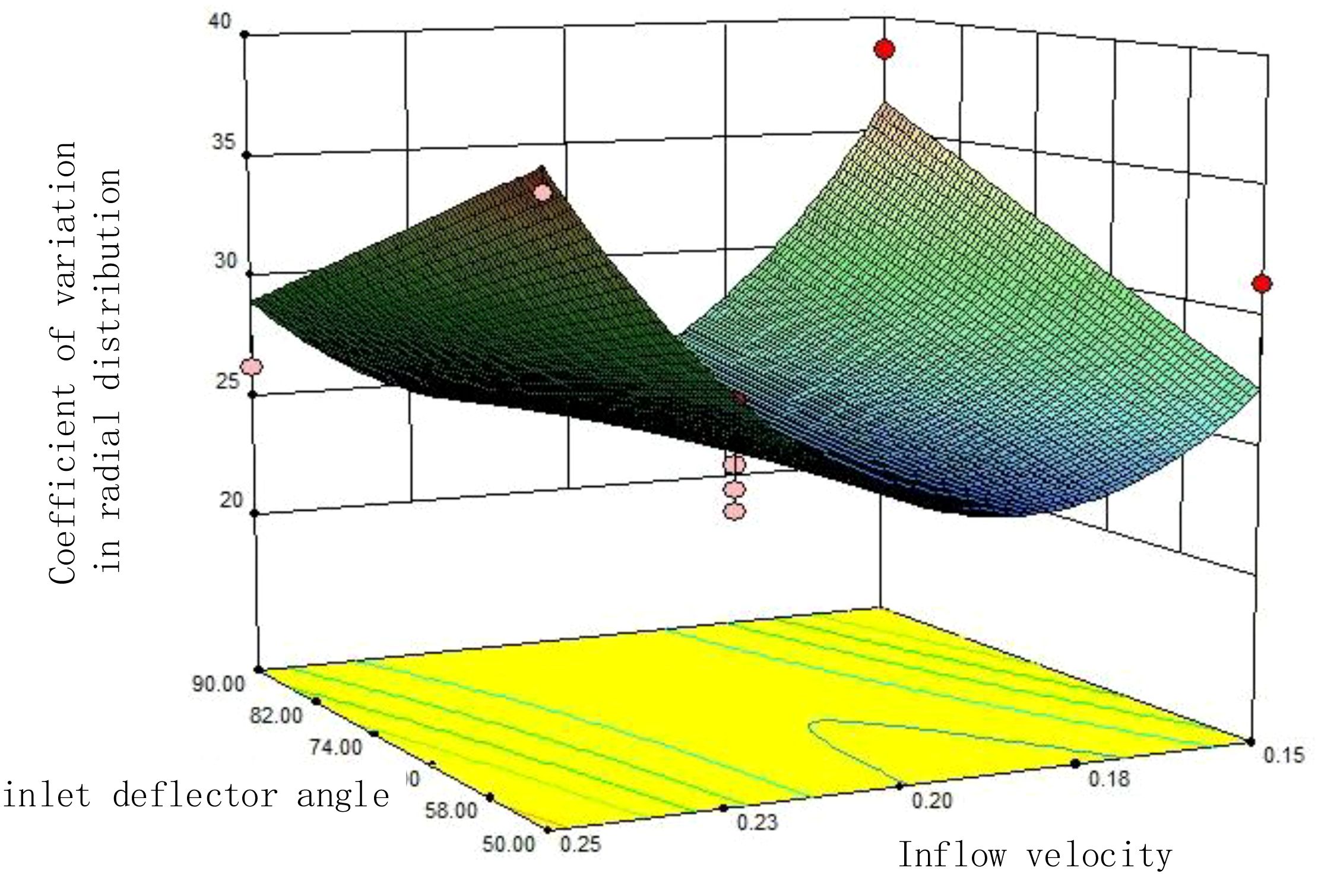
Figure 12 Response surface diagram.
The parameters of culture cone operation, such as inflow velocity (v), cultivation density (τ), and inlet deflector angle (α), have a significant impact on the distribution of D-shaped larvae. After determining the structure parameters of the culture cone, in order to further improve the spatial distribution uniformity of D-shaped larvae, the optimization objective is to minimize the variation coefficients of the radial and axial distribution of D-shaped larvae. The inlet deflector angle is limited to 50°~90°, the inflow velocity is limited to 0.15 m/s~0.35m/s, and the cultivation density ratio is limited to 100/ml~300/ml. The regression model is solved to obtain the optimal parameter combination, and the relevant constraint conditions are shown in the Equation 11.
The optimal combination function in Design-Expert is used to solve the regression model. When the inflow velocity is 0.19m/s, the cultivation density is 110 pcs/mL, and the inlet deflector angle is 60.94°, the experimental factor parameter combination is the best, the measured radial coefficient of variation for D-shaped larvae was 22.13%, and the axial coefficient of variation was 36.72%. The measured value of radial variation coefficient decreased by 43.14% compared to the simulation value, the reason for this is that the addition of an inlet deflector in the experiment improved the radial distribution uniformity of water flow in the culture cone, significantly improving the distribution uniformity of D-shaped larvae in the culture cone; the error between the measured and simulated values of the axial coefficient of variation is 4.41%, indicating that the fluid structure coupling simulation model established in this paper has good accuracy and can be used for optimizing the design of scallop larval culture devices.
1. This paper presents the design of an upwelling recirculating water system for scallop larval cultivation. Single-factor simulation experiments were conducted to investigate the distribution patterns of D-shaped larvae within the culture cone(θ). The primary factors affecting the distribution of D-shaped larvae were identified as the bottom cone angle, the column height/cone height ratio(n), and the inflow velocity(v);
2. A research of secondary rotation orthogonal experiment was conducted, the variance analysis and response surface analysis on the experimental results were performed using Design Expert software. The results indicate that the inflow velocity(v), bottom cone angle(θ), and column height/cone height ratio(n) have an extremely significant impact on the radial coefficient of variation of D-shaped larvae (P<0.01). The quadratic term of the inflow velocity(v), the bottom cone angle(θ) and its quadratic term, and the interaction between the bottom cone angle (θ) and the column height/cone height ratio (n) have an extremely significant impact on the axial coefficient of variation (P<0.01), the optimal structural parameters were determined using Design Expert software;
3. Conducted experimental research on scallop larval cultivation system. A secondary rotation orthogonal experiment was conducted to research the pattern of effects of inlet deflector angle(α), inflow velocity(v), and cultivation density(τ) on the spatial distribution uniformity of scallop larvae, determine the optimal operational parameters of an inlet deflector angle(α) of 60.94°, an inflow velocity(v) of 0.19 m/s, and a cultivation density(τ) of 110 pcs/mL. The inlet deflector improved the radial distribution uniformity of water flow inside the culture cone, the radial distribution coefficient of variation of D-shaped larvae reaches 21.28%, the coefficient of variation in axial distribution is 36.72%,and the error between the measured value and simulated values is 4.41%.
4. This study used flowing water cultivation, with a cultivation density of up to 110 pcs/ml, which is 9.17 times higher than that of still water cultivation. The cultivation density has been significantly increased, but this study did not consider the impact of high cultivation density on the growth and development of D-shaped larvae. Subsequent experimental studies can be conducted to determine the impact of cultivation density on the hatching rate and growth rate of D-shaped larvae, in order to achieve the best cultivation effect.
5. The up-flow circulating water cultivation system designed in this article significantly improves the cultivation density of scallop larvae, effectively saving cultivation water and reducing labor costs. However, scallop larval cultivation is a complex process, and precise control of parameters such as temperature, dissolved oxygen, and liquid level is also required during the cultivation process. It is recommended to implement remote monitoring and control of scallop larval cultivation process based on Internet of Things technology in the future.
The original contributions presented in the study are included in the article/supplementary material. Further inquiries can be directed to the corresponding author.
XL: Conceptualization, Project administration, Supervision, Writing – review & editing. YY: Methodology, Software, Writing – original draft. DL: Writing – review & editing. SC: Software, Writing – original draft. SW: Software, Writing – review & editing. XY: Writing – original draft. ZL: Writing – original draft. YW: Writing – review & editing. HZ: Methodology, Writing – review & editing.
The author(s) declare financial support was received for the research, authorship, and/or publication of this article. This research was funded by National Key R&D Program of China (2023YFD2400800); Unveiling and Commanding Project of Dalian(2021JB11SN035); Education Department of Liaoning Province (LKMZ20221112);”Azure Scholar” Project of Dalian Ocean University(for Hanbing Zhang); Key Laboratory of Environment Controlled Aquaculture (Dalian Ocean University) Ministry of Education(202212).
The authors declare that the research was conducted in the absence of any commercial or financial relationships that could be construed as a potential conflict of interest.
All claims expressed in this article are solely those of the authors and do not necessarily represent those of their affiliated organizations, or those of the publisher, the editors and the reviewers. Any product that may be evaluated in this article, or claim that may be made by its manufacturer, is not guaranteed or endorsed by the publisher.
An C. H., Sin M. G., Kim M. J., Jong I. B., Song G. J., Choe C., et al. (2018). Effect of bottom drain positions on circular tank hydraulics: CFD simulations. Aquacultural Eng. 83, 138–150. doi: 10.1016/j.aquaeng.2018.10.005
Cao S., Wang J., Wang Q., Liang W., Yin M., Liu G., et al. (2017). Artificial breeding of introduced rock scallop Crassadoma gigantea. J. Dalian Ocean Univ. 32, 1–6. doi: 10.16535/j.cnki.dlhyxb.2017.01.001
Cary S. C., Leighton D. L., Phleger C. F. (1981). Food and feeding strategies in culture of larval and early juvenile purple-hinge rock scallops, Hinnites multirugosus (GALE). J. World Mariculture Soc. 12, 156–169. doi: 10.1111/j.1749-7345.1981.tb00252.x
Chen L., Zhang D., Chen W. (2014). Numercial simulation and test on two-phase flow inside shell of transfer case based on fluid-structure interaction. Trans. Chin. Soc. Agric. Eng. 30, 54–61. doi: 10.3969/j.issn.1002-6819.2014.04.008
Dauda A. B., Ajadi A., Tola-Fabunmi A. S., Akinwole A. O. (2019). Waste production in aquaculture: Sources, components and managements in different culture systems. Aquaculture Fisheries 4, 81–88. doi: 10.1016/j.aaf.2018.10.002
Garcia A. B., Kamermans P. (2015). Optimization of blue mussel (Mytilus edulis) seed culture using recirculation aquaculture systems. Aquaculture Res. 46, 977–986. doi: 10.1111/ARE.12260
Gorle J. M. R., Terjesen B. F., Mota V. C., Summerfelt S. (2018). Water velocity in commercial RAS culture tanks for Atlantic salmon smolt production. Aquacultural Eng. 81, 89–100. doi: 10.1016/j.aquaeng.2018.03.001
Hu J., Ouyang H., Sun Y., Yan X., Zhu H. (2016). Differential analysis of scallop aquaculture between China and Japan. World Agric. 06, 115–120. doi: 10.13856/j.cn11-1097/s.2016.06.020
Jorgensen L. (1987). An automated system for incubation of pelagic fish eggs. Modeling Identification Control 8, 47–50. doi: 10.4173/mic.1987.1.6
Labatut R. A., Ebeling J. M., Bhaskaran R., Timmons M. B. (2015). Modeling hydrodynamics and path/residence time of aquaculture-like particles in a mixed-cell raceway (MCR) using 3D computational fluid dynamics (CFD). Aquacultural Eng. 67, 39–52. doi: 10.1016/j.aquaeng.2015.05.006
Lin Z., Chai X., Xiao G., Zhang J., Fang J., Wu H., et al. (2005). “Research on cultivating bivalve juveniles utilizing upwelling systems,” in 12th Academic Symposium of the Chinese Association of Oceanic Limnology and the Malacological Society of China, Vol. 09 (Taiyuan, China).
Liu X. (2008). A new type of incubator - aerated hatching net tube for fish fry. Shandong Fisheries 04), 30.
Liu X., Hu L., Zhang Y. (2016). Analysis of common issues in artificial cultivation of bay scallop juveniles and corresponding measures. Ocean Fishery 9, 64–66.
Liu Y., Zheng J., Qiu T. (2014). Research and development status and trends of shellfish aquaculture facilities engineering. Fishery Modernization 05, 1–5. doi: 10.3969/j.issn.1007-9580.2014.05.001
Mi G., Lian Q., Wei X. (2009). Floating aeration system for fish fry incubation experiment. Fishery Modernization 36, 50–53.
Rico-Villa B., Woerther P., Mingant C., Lepiver D., Pouvreau S., Hamon M., et al. (2008). A flow-through rearing system for ecophysiological studies of Pacific oyster larvae. Aquaculture 282, 54–60. doi: 10.1016/j.aquaculture.2008.06.016
Shi M. (2018). CFD simulation and optimization of multiphase flow in recirculating biofloc technology system (Hangzhou: Zhejiang University).
Spreitzenbarth S., Jeffs A. (2020). Egg survival and morphometric development of a merobenthic octopus, Octopus tetricus, embryos in an artificial octopus egg rearing system. Aquaculture 526. doi: 10.1016/j.aquaculture.2020.735389
Subhan U., Iskandar Z., Panatarani C., Joni I. M. (2022). Effect of ultrafine bubbles on various stocking density of striped catfish larviculture in recirculating aquaculture system. Fishes 7, 190. doi: 10.3390/fishes7040190
Xu X., He M. (2010). Experimental design and application of design-expert and SPSS[M] (Beijing: Science Press).
Keywords: scallop larvae, water-recirculating cultivation system, deflector, coupling simulation, uniformity of distribution
Citation: Li X, Yang Y, Liu D, Chen S, Wu S, Yuan X, Liu Z, Wang Y and Zhang H (2024) Optimization of recirculating water scallop larval cultivation system based on EDEM-fluent coupling. Front. Mar. Sci. 11:1407670. doi: 10.3389/fmars.2024.1407670
Received: 27 March 2024; Accepted: 15 July 2024;
Published: 29 July 2024.
Edited by:
Fukun Gui, Zhejiang Ocean University, ChinaReviewed by:
D. K. Meena, Central Inland Fisheries Research Institute (ICAR), IndiaCopyright © 2024 Li, Yang, Liu, Chen, Wu, Yuan, Liu, Wang and Zhang. This is an open-access article distributed under the terms of the Creative Commons Attribution License (CC BY). The use, distribution or reproduction in other forums is permitted, provided the original author(s) and the copyright owner(s) are credited and that the original publication in this journal is cited, in accordance with accepted academic practice. No use, distribution or reproduction is permitted which does not comply with these terms.
*Correspondence: Hanbing Zhang, emhhbmdoYW5iaW5nQGRsb3UuZWR1LmNu
Disclaimer: All claims expressed in this article are solely those of the authors and do not necessarily represent those of their affiliated organizations, or those of the publisher, the editors and the reviewers. Any product that may be evaluated in this article or claim that may be made by its manufacturer is not guaranteed or endorsed by the publisher.
Research integrity at Frontiers
Learn more about the work of our research integrity team to safeguard the quality of each article we publish.