Beyond counting calls: estimating detection probability for Antarctic blue whales reveals biological trends in seasonal calling

We explore the utility of estimating the density of calls of baleen whales for better understanding acoustic trends over time. We consider as a case study stereotyped ‘song’ calls of Antarctic blue whales (Balaenoptera musculus intermedia) on their Antarctic feeding grounds over the course of a year-long, continuous recording from 2014. The recording was made in the Southern Ocean from a deep-water autonomous hydrophone moored near the seafloor in the Eastern Indian sector of the Antarctic. We estimated call density seasonally via a Monte-Carlo simulation based on the passive sonar equation, and compared our estimates to seasonal estimates of detection rate, which are commonly reported in acoustic studies of Antarctic blue whales. The resulting seasonal call densities at our Antarctic site were strongly influenced by seasonally varying noise levels, which in turn yielded seasonal differences in detection range. Incorporating the seasonal estimates of detection area into our analysis revealed a pattern of call densities in accord with historic (non-acoustic) knowledge of Antarctic blue whale seasonal distribution and migrations, a pattern that differed from seasonal detection rates. Furthermore, our methods for estimating call densities produced results that were more statistically robust for comparison across sites and time and more meaningful for interpretation of biological trends compared to detection rates alone. These advantages came at the cost of a more complex analysis that accounts for the large variability in detection range of different sounds that occur in Antarctic waters, and also accounts for the performance and biases introduced by automated algorithms to detect sounds. Despite the additional analytical complexities, broader usage of call densities, instead of detection rates, has the potential to yield a standardized, statistically robust, biologically informative, global investigation of acoustic trends in baleen whale sounds recorded on single hydrophones, especially in the remote and difficult to access Antarctic.

1 Introduction

Underwater passive acoustic monitoring has for decades been proposed as an efficient means of studying certain vocal marine species, particularly cetaceans (Mellinger et al., 2007; Van Parijs et al., 2009) with many applications focusing on understanding distribution and movement patterns of particular species. In more recent years, advances in computing, acoustic, and statistical methods have seen an increasing trend towards local density estimation from passive acoustics (Thomas and Marques, 2012; Wilcock, 2012; Harris et al., 2013, 2018; Helble et al., 2013; Hildebrand et al., 2015).

Density estimation can ultimately lead us to make assessments across multiple recording sites (Helble, 2013) that can lead to understanding broader population trends in space and time. Estimating animal density from underwater passive acoustic monitoring data can be a significant challenge given uncertainties in detection range of listening stations, acoustic behaviour of animals, and the performance of automatic detectors of animal sounds, among others.

A variety of acoustic techniques have been proposed and summarized in a review by Marques et al. (2013), and most of these methods are derived from widely used (predominantly visual) methods for estimating abundance (e.g. Borchers et al., 2002). Here we present an application of one of these methods: estimating density from single fixed passive acoustic sensors with a detection function estimated from auxiliary data (Küsel et al., 2011; Marques et al., 2013 Section IV.3). Specifically, our application focuses on estimating the seasonal density of calls, (henceforth call density) of Antarctic blue whales (Balaenoptera musculus intermedia; henceforth ABWs) on their Antarctic feeding grounds.

ABWs, the largest animal to have ever lived, are critically endangered (Cooke, 2018) after being hunted to the brink of extinction during industrial whaling (Rocha et al., 2015). They were subsequently encountered very rarely during three decades of visual surveys spanning the 1970s-2000s (Branch, 2007), and for the past two decades much of the primary data collection on this species has relied on passive acoustics (e.g. Ljungblad et al., 1998; Širović et al., 2004, 2009; Rankin et al., 2005; Širović and Hildebrand, 2011; Gavrilov et al., 2012; Balcazar et al., 2015; Miller et al., 2015, 2017, 2019; Rocha et al., 2015; Tripovich et al., 2015; Leroy et al., 2016; Shabangu et al., 2017, 2019, 2020; Thomisch, 2017; Dréo et al., 2019; Letsheleha et al., 2022). The low frequency sounds of baleen whales, particularly blue and fin whales, have long been known to be detectable over very large areas (Payne and Webb, 1971; Širović et al., 2007; Miller et al., 2015). Work to quantify site- and time-specific detection ranges (e.g., McDonald and Fox, 1999; McCauley et al., 2001; Samaran et al., 2010a; Shabangu et al., 2020), and this has confirmed that detection range can vary across sites and timespans. However, relatively few acoustic studies have focused on quantifying and accounting for this variability in detection range, despite the importance of these factors when interpreting counts of acoustic detections. More recently, several of the underwater acoustic studies that have taken detection range and its variability into account have done so via estimation of call densities (e.g. Helble et al., 2013; Harris et al., 2018; Miksis-Olds et al., 2019; Oedekoven et al., 2021; Warren et al., 2021), though none of these studies have focused on the calls of ABWs in the extremely variable Antarctic environment.

Call densities are one-step removed from acoustic estimates of animal density in that call densities do not account for vocal behaviour of animals. Therefore, call densities should be interpreted as indicative of a potential combination of animal density and animal behaviour. Call densities are similar to detection rates (call-counts per unit time), which have been commonly reported in many prior passive acoustic studies of ABWs (Širović et al., 2009; Samaran et al., 2013; Balcazar et al., 2015; Leroy et al., 2016; Thomisch, 2017; Dréo et al., 2019; Shabangu et al., 2020). However, unlike detection rate, call density is standardised by detection area yielding units of calls per unit area per unit time. Detection range of low-frequency whale sounds can be highly variable across sites and over time (Samaran et al., 2010a; Harris et al., 2018; Shabangu et al., 2020), so by accounting for all the main factors that influence detection, including the performance of an automated detector (i.e. false positives and missed-detections), resulting call densities do not suffer from one of the biggest hindrances to interpreting detection rates from these previous studies.

Here we describe a method to estimate seasonal call densities of ABW sounds, and results are standardized and suitable to assess trends in space and time. We also describe and apply methods to estimate the coefficient of variation (CV) of each of our call density estimates, and this in turn facilitates statistically robust comparisons among different regions and/or timespans.

2 Methods

2.1 Data collection

Acoustic recordings for our application come from the Australian Antarctic Division’s long-term acoustic monitoring dataset (Miller et al., 2021c), which is part of the Southern Ocean Hydrophone Network (Opzeeland et al., 2013). We focus on the site located on the Southern Kerguelen Plateau (62.38°S, 81.79°E) and the year 2014, as this site and year contain near-continuous acoustic recording, and already contained a representative subset of 4298 ground-truth annotations of ABW song calls made by an expert analyst (Miller et al., 2020, 2021a). Recording for the full dataset started on February 10, 2014 and ended on February 7, 2015, totalling approximately 8700 hours of underwater sound.

2.2 Analysis

In general we follow the methods described in Harris et al. (2024, submitted), which were in turn extended from Küsel et al. (2011) to use auxiliary data to estimate the probability of detecting a call, which is a key parameter in density estimation methods. We apply the density estimation formula (Equation 1) for a single-sensor (a single fixed listening station with a single hydrophone) with call-counts, $n_c$, generated from an automated detector that has a false discovery rate $\widehat{f}$, such that:

$\begin{array}{ll}{\widehat{D}}_c=\frac{n_c(1-\widehat{f})}{A{\widehat{p}}_{a}T}& (1)\end{array}$

Here ${\widehat{D}}_c$ is the estimated call density; A is the sum of the area for each transect; T is the duration of recording (in h); ${\widehat{p}}_a$ is the probability of detection in the study area; and the circumflex or “hat operator” (^) indicates that a quantity is an estimated parameter. The following sections describe how each of these quantities were obtained.

2.2.1 Duration of recording ($T$)

Here we were interested in determining whether there were seasonal differences in call density, and how these compared to seasonal estimates of detection rate. To facilitate this we split the dataset into five time periods: four seasonal estimates and one annual estimate. Seasons were defined as summer comprising months: Dec, Jan, Feb; autumn: Mar, Apr, May; winter: Jun, Jul, Aug; and spring: Sep, Oct, Nov, and ‘full year’ included all of the data from each season. We opted for a conventional definition of seasons to enable comparisons with other ecological and biological studies using this approach, rather than relying on a physical oceanographic method, which can be region-specific. Each of the following quantities were then estimated independently for each time period, with T measured directly as the duration of recorded audio for each period.

2.2.2 Number of calls ($n_c$)

To count the number of calls we applied a spectrogram correlation detector to the entire duration of recorded data. This detector targets ABW song calls, also known as “Z-calls” (Širović et al., 2004), which are made up of unit A (the constant tone comprising the top of the Z), unit B, (the downsweep that connects units A & C), and unit C (the near-constant or slightly downswept tone comprising the bottom of the Z, Rankin et al., 2005). The detector we used is the same as the Antarctic blue whale “ABZ” call detector described by Miller et al. (2021a). According to the ground-truth detections (i.e., manual annotations made by an expert analyst), this spectrogram-correlation detector had mediocre performance (Miller et al., 2021a), but was capable of detecting calls composed of stand-alone unit-A, calls with only units A & B visible, and full Z-calls that contained all three units: A, B, and C (Figure 1). We chose a detection threshold that had a low false positive rate (approximately 2.5 false positives per hour), but also had a low true positive rate of approximately 0.27 for this site-year. Here, the true positive rate (AKA recall) was defined as the proportion of manually annotated detections found by the automated detector.

Figure 1

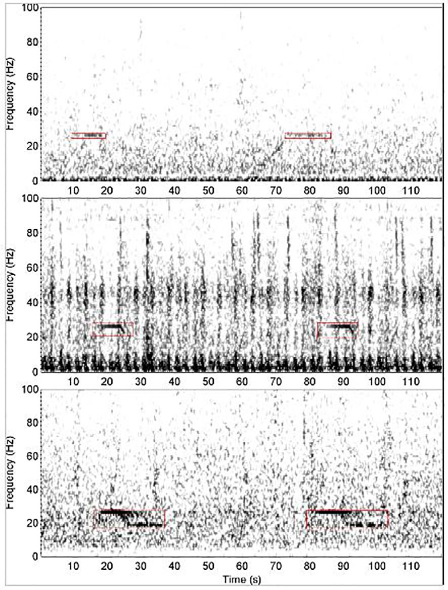
Figure 1. Examples of Antarctic blue whale song calls. Top: two detections of stand-alone unit-A. Middle: two detections that appear to consist solely of units A and B. Bottom: two Z-calls containing units A, B, & C. Image reproduced from (Miller et al., 2021a) under a creative-commons licence.

2.2.3 False discovery rate ($\widehat{f}$)

False discovery rate for each season was calculated by expert inspection of every 50th automated detection throughout the dataset. We applied a fixed interval for manual inspection to ensure a consistent examination of a subset of automated detections across the dataset. The expert analyst, author FRC, viewed a spectrogram of the detection, and then determined whether or not that detection was true positive, or a false positive. The total number of true positives, TP, and false positives, FP, were then tabulated for each time period in order to estimate the false discovery rate (Equation 2):

$\begin{array}{ll}\widehat{f}=FP/(FP+TP)& (2)\end{array}$

2.2.4 Probability of detecting a call within the study area (${\widehat{p}}_a$)

Detection probability was estimated with a Monte Carlo simulation using elements of the passive sonar equation. The method is described in full in Harris et al. (2024, submitted) and a summary is provided here. There were two main parts to the analysis: first, detection probability was modelled as a function of call signal-to-noise ratio (SNR) using a shape-constrained generalised additive model (GAM). Second, a Monte Carlo simulation was used to estimate the average detection probability ${\widehat{p}}_a$ needed for Equation 1. The simulation was populated with virtual blue whale calls around a single omnidirectional hydrophone. All virtual calls were assigned source levels (SL), ambient noise levels (NL) and a transmission loss (TL), given their virtual position was known in relation to the hydrophone. The SNR (in dB) for unit-A of each simulated call was calculated using the expression from the passive sonar equation (Equation 3):

$\begin{array}{ll}\mathrm{SNR}=\mathrm{SL}-\mathrm{TL}-\mathrm{NL}& (3)\end{array}$

A predicted detection probability for each call was estimated using the GAM results, and then the average detection probability, ${\widehat{p}}_a$, was estimated from all the simulated calls (see section Monte Carlo method below for additional details).

2.2.4.1 Detector characterisation curves (SNR-detection functions)

The data from the IWC-SORP annotated library (Miller et al., 2020) for the site-year S. Kerguelen Plateau-2014 were used to estimate the probability of detection as a function of SNR (AKA detector characterisation curves, Figure 2), which illustrates the estimated relationship between SNR and probability of detection, essential for assessing how effective and reliable a detection system is under different levels of noise interference. As in Miller et al. (2021a) the 4298 detections of unit-A, units A-B and Z-calls from the manual analyst were treated as ground-truth, and false-positive detections from the automated detector were removed prior to modelling the relationship. The model here was similar to that presented by Miller et al. (2021a), however, here we estimated the SNR as SNR=RL-NL (in dB) and we did not divide by the variance of the noise as in the previous work (Miller et al., 2021a). Furthermore, here the relationships between SNR and automated detections were modelled independently for each season and the full year, whereas in the previous work only a single model was created for the full year. The detector characterisation curves were modelled as binomial shape-constrained GAMs with logit link functions and 5 ‘knots’ using the package ‘scam’ (Pya, 2022) in R version 4.2.0 (R Core Team, 2019) using the formula (Equation 4):

Figure 2

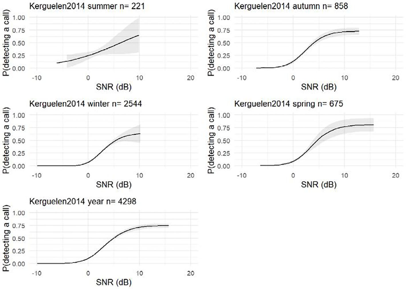
Figure 2. Probability of detecting a call given a signal-to-noise ratio (SNR) using a separate shape-constrained generalised additive model (GAM) for each time period. The grey area around each curve depicts the 95% confidence limits.

$\begin{array}{ll}\mathrm{detected}\sim \text{s}(\mathrm{SNR})& (4)\end{array}$

Here, “detected” was a Boolean response variable with value 1 or 0 depending on whether or not the automated detector had any temporal overlap with a ground-truth manual annotation; SNR was the predictor variable, measured from the acoustic data as defined above.

2.2.4.2 Source levels

For the Monte Carlo simulation, SL was modelled as normally distributed (in dB), with a mean of 189 dB re 1 μPa @1m and standard deviation of 8.0. There have been very few studies of SL of ABW sounds, but they all report mean SL of unit-A that are very close to this value (Širović et al., 2007; Samaran et al., 2010b; Bouffaut et al., 2021; Miller et al., 2021b), despite these studies all being conducted in different seasons. Thus, the same distribution of SL was used for all time periods. The standard deviation of SL used was that reported by Miller et al. (2021a), which has the largest sample size of all these studies in terms of both number of calls (350) and likely number of whales.

2.2.4.3 Transmission-loss modelling

Transmission-loss (TL) was modelled by applying the parabolic equation method via the RAMGeo acoustic propagation algorithm (Collins, 2002, Figure 3). This was implemented via the software package AcTUP (Duncan, 2005), which is a user interface to the 2005 version of the Ocean Acoustics Library (Porter, 2020). TLs were modelled for a frequency of 26 Hz (corresponding to unit A of ABW calls) along 24 evenly-spaced radial transects originating at the recorder, and ending at distance w along each bearing with a distance increment of 2 m following the principle of reciprocity of TL between source and receiver (Nghiem‐Phu and Tappert, 1985; Jensen et al., 2011).

Figure 3

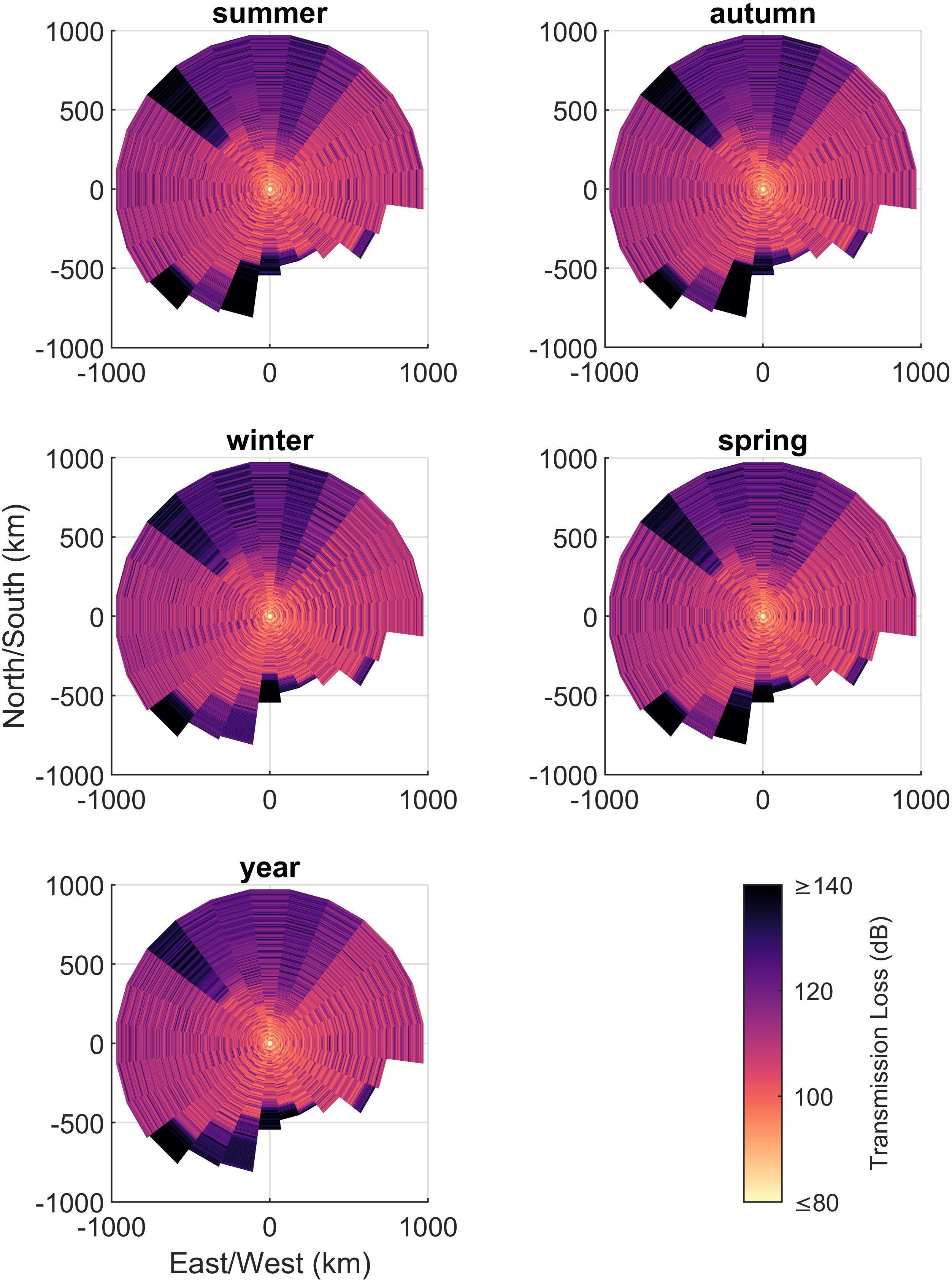
Figure 3. Transmission loss, TL, model per profile: 0-345° in 15° increments, respectively plotted for each season. TL were modelled at a frequency of 26 Hz assuming whale depth of 25 m and recorder depth of 1800 m.

Parameters for the TL model included the depth at which the call was produced and received, bathymetry, seabed acoustic properties, and water-column sound-speed profile (Figure 4). The depth of the recorder was estimated to be 1800 m using the ship’s echosounder during deployment, and the depth of calling was estimated to be 25 m, identical to that for which SL estimates were made (Miller et al., 2021b). We assumed that the effects of small variations in the depth of the calling whale, which can have large effects on the TL, were potentially counterbalanced by the SL adopted in this study, since such effects were taken into account in the SL estimation. Bathymetry was extracted for each transect from the etopo1 database at 10 km distance increments (Amante and Eakins, 2009). Seabed acoustic properties were modelled as large-grain with a compressional sound speed of 1520 m/s and a density of 1200 kg/m3. These properties were similar to typical parameters for a homogenous seabed made of “clay” (Lurton, 2010). Only limited in-situ spatial information on geoacoustic properties of the seabed in the region could be found, but a ‘clay’ seabed seemed to be a reasonable choice according to the few data products available (Dutkiewicz et al., 2015) (Figure 4).

Figure 4

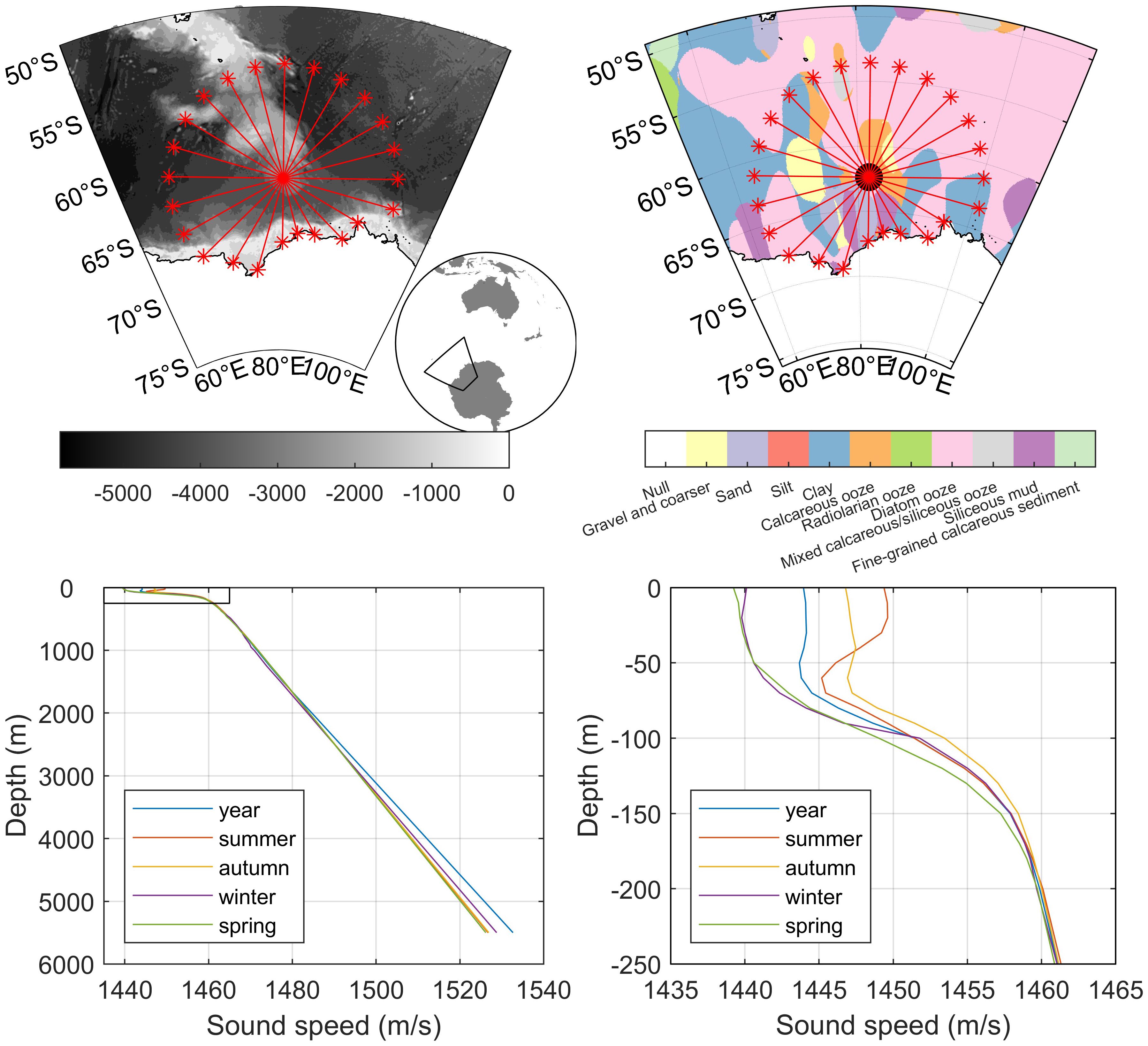
Figure 4. Maps of recording location (red circle) and transects used to estimate probability of detection in the study area (red lines). Top Left: bathymetry in m from etopo1 (Amante and Eakins, 2009). Top Right: sediment type from the Census of Seabed Sediments (Dutkiewicz et al., 2015) illustrating that the most common sediments are “clay” and “diatom ooze.” Bottom: seasonal sound-speed profiles at the recording location as a function of depth derived salinity and temperatures from the World Ocean Atlas 2018 (Boyer et al., 2018). Bottom left panel shows full depth range, while the bottom right panel shows the same information, but focused on the first 250 m to better illustrate the details of this region.

A single sound-speed profile (SSP) for each season (summer, autumn, winter, spring), and a single SSP for the full year was created from the World Ocean Atlas 2018 (Boyer et al., 2018) using the respective seasonal and yearly salinity and temperature water column profiles nearest in location to the instrument. The GSW Oceanographic Toolbox was used to calculate sound-speeds from salinity, temperature, and depth (McDougall and Barker 2011). Atmospheric seasons were chosen instead of physical oceanographic seasons as they are typically observed when discussing seasonality in marine mammals. However, the difference in SSP between atmospheric and oceanographic seasons, which are offset by a month, was not expected to substantially affect TL in this application and region. This is because Antarctic SSPs are upward refracting and contain shallow sound speed minima throughout the year, and thus are relatively stable across seasons compared to more temperate regions.

2.2.4.4 Noise levels

Noise levels were estimated for each manually annotated detection by calculating the mean power in dB re: 1 µPa in the 25-29 Hz frequency band of the spectrogram (i.e. the frequency band of SL measurements of unit-A of ABW song calls). The NL was measured 26 seconds (25 seconds + 1 second) prior to the onset of manual detection. When the annotation was at the beginning of the file, without 26 seconds of preceding audio, the noise was measured immediately following the detection. NL were measured for each call regardless of the presence or absence of other calls, and regardless of the presence or absence of a ‘chorus’ (i.e., elevated levels in the call band that arise from the hydrophone receiving multiple overlapping calls from many non-localisable and/or distant animals). This decision can be viewed as a choice to explicitly include the effects of the ‘chorus’ and the potential effects of masking from other calls as noise in our estimates of call density. The mean and standard deviation of measured NL for each season and the full year were then used as input parameters (i.e., to generate normal distributions of NL) for Monte-Carlo simulations for the respective time-periods.

2.2.4.5 Monte Carlo method

A Monte Carlo simulation similar to the method described in Harris et al. (2024, submitted) was used to estimate average detection probability, and is summarised here. The simulation has two stages referred to as the outer- and inner loops. The two stages are necessary to appropriately account for all sources of variability in the simulation.

In the outer loop, different source level and ambient noise level distributions were simulated, as well as a detector characterisation curve using parametric bootstraps. Normal distributions were assumed for the source- and noise level distributions with mean and standard deviations as described above, as the dB values were normally distributed in Miller et al. (2021b). A multivariate normal distribution was assumed for the model coefficients from the GAM. The estimated coefficient parameters were used as the mean values and the variance was derived from the GAM covariance matrix. The outer loop was run 1000 times, generating 1000 separate distributions for source- and noise level and 1000 detector characterisation curves. Each combination of simulated source- and noise level distributions, and the detector characterisation curve, were used to run the inner loop. The parametric bootstrap in the outer loop was intended to conservatively preserve variability and expand the range of uncertainty, particularly for SL. Though we used the best available estimates of SL, these estimates still came from a small number of whales and locations. The bootstrap aims to expand the 8 dB standard deviation around the mean SL to better model the uncertainty of these estimates.

In the inner loop, virtual whale calls were placed at 100 m range steps along each transmission loss transect (maximum range = 980 km, with land truncating some transects), resulting in a maximum of 9,800 virtual whale calls per transect. Each call was assigned a source level and an ambient noise level using a random draw from the simulated source- and noise level distributions. Then the relevant transmission loss value was used to estimate the simulated SNR of the call as expected at the hydrophone. The detector characterisation curve was then used to estimate the detection probability for each call, given their SNR values. An average detection probability, ${\widehat{p}}_a$, was then estimable for each transect for each run of the inner loop (averaged across the maximum number of calls per transect, weighted by range, to account for the increasing area represented by calls at increased ranges along the radial). Additionally, we computed the overall detection probability as a weighted mean, with weights based on the area of each transect.

2.2.4.6 Estimation of CV

The delta method (Seber, 1982) was used to estimate an associated CV for each density estimate. For this, the CVs of each component of the analysis that contributed to the uncertainty in the eventual density estimate were combined to produce an overall CV for the D_c. These components were the probability of detection, the encounter rate and the false discovery rate. A CV is defined as the standard deviation divided by the mean estimate. Therefore, given ${\widehat{p}}_a$ was a mean value, the standard error of ${\widehat{p}}_a$ was divided by ${\widehat{p}}_a$. The CV for $\widehat{f}$ was estimated in the same way. For $n_c$, the standard deviation was used since the encounter rate was not considered to be a mean estimate. For $\widehat{f}$, CV was estimated computing the variance of a weighted mean following the definition of Cochran (1977).

3 Results

3.1 Pre-processing of data for call density estimates

The automatic detector yielded 77905 detections, across 8640.2 hours of recording, corresponding to the total time of deployment. Of these, 1559 automated detections were used to estimate false discovery rate, $\widehat{f}$, with 313 from summer, 453 from autumn, 563 from winter, and 230 from spring. For the full year of deployment, $\widehat{f}$ was 0.314. The detections per season, and other seasonal inputs into the call density estimates are presented in Table 1.

Table 1

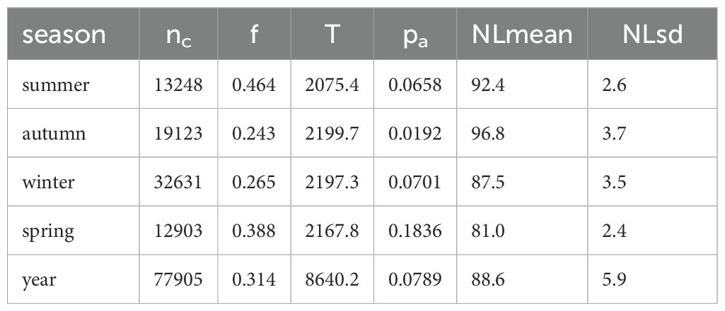
Table 1. Inputs into the call density equation for each season: number of detections (n_c), time of recording (T) in h, false discovery rate (f), probability of detection (p_a), and parameters for the distribution of noise level (NL) in dB re 1 µPa² RMS.

Noise levels showed strong differences over time yielding differences in seasonal mean NLs and respective standard deviations (Table 1; Figure 5). These seasonal differences in NL are in accord with what would be expected due to the seasonal effects of Antarctic sea-ice on underwater noise levels (Miller et al., 2016; Menze et al., 2017; Shabangu et al., 2020; Yun et al., 2021). However, the distribution of SNR of the annotated calls was relatively consistent over time (Figure 5). In contrast to NL, the SNR-detection functions for autumn, winter, and spring were all fairly similar to each other, but different than that for summer (Figure 2). In particular, the SNR-detection function for summer had a shallower slope than other seasons, and substantially wider confidence intervals.

Figure 5

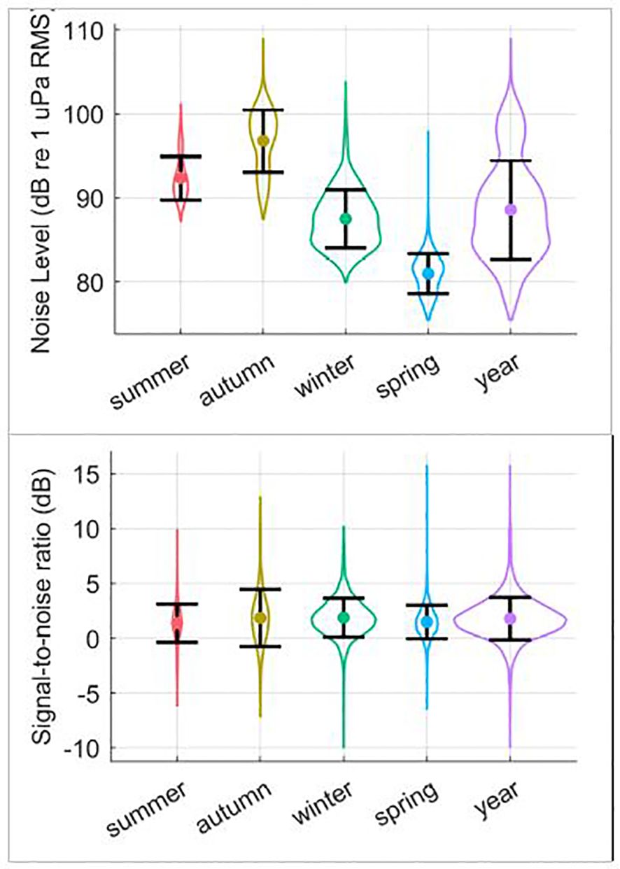
Figure 5. Top: Noise level (NL) and bottom: signal-to-noise ratio (SNR) distributions measured for unit-A of the manually annotated Antarctic blue whale A, B, and Z-calls (25-29 Hz band). Violin plots show the distributions of values from ground-truth detections, while error-bars show the standard deviation centred on the mean value.

The probability of detection produced by the Monte Carlo simulation decreased to a negligible value at the adopted maximum range of 980 km (Figure 3). Following the pattern set out by NL, the probability of detection within the study area, ${\widehat{p}}_a$, varied substantially across the different time periods (Figure 6; Table 1). The lowest ${\widehat{p}}_a$ occurred in autumn and the highest ${\widehat{p}}_a$ values were in spring and, as would be expected, these were inversely correlated with NL.

Figure 6

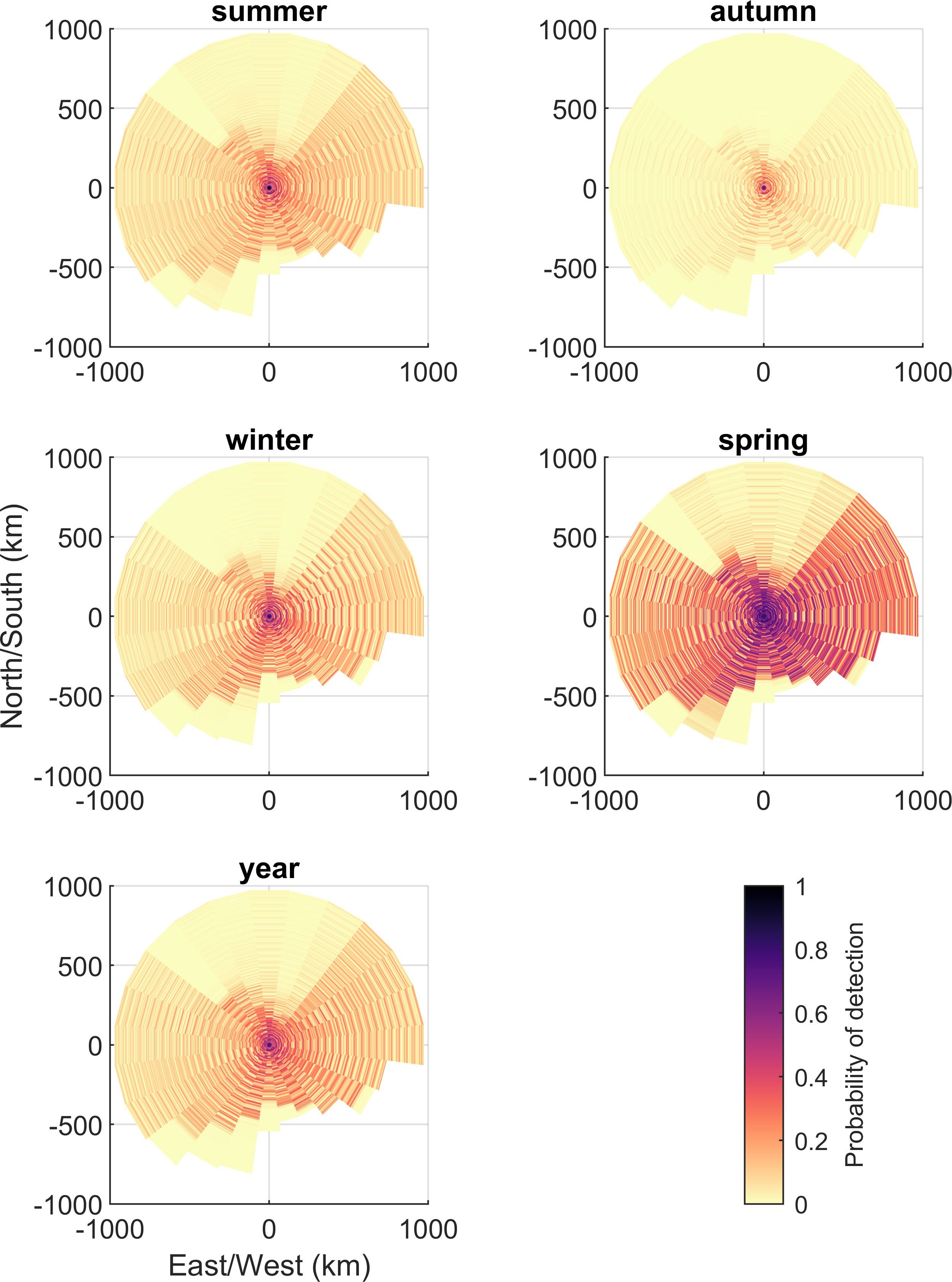
Figure 6. Probability of detection, ${\widehat{p}}_a$, within study area for each radial transect.

3.2 Seasonal density estimates

Seasonal call densities, ${\widehat{D}}_c$, ranged from 0.007 calls/h/1000 km² in spring to 0.128 in autumn. The CV of call density was highest in autumn (CV=0.153), and lowest in summer (CV=0.112), but with only small differences in CV among time periods (Figure 7; Table 2).

Figure 7

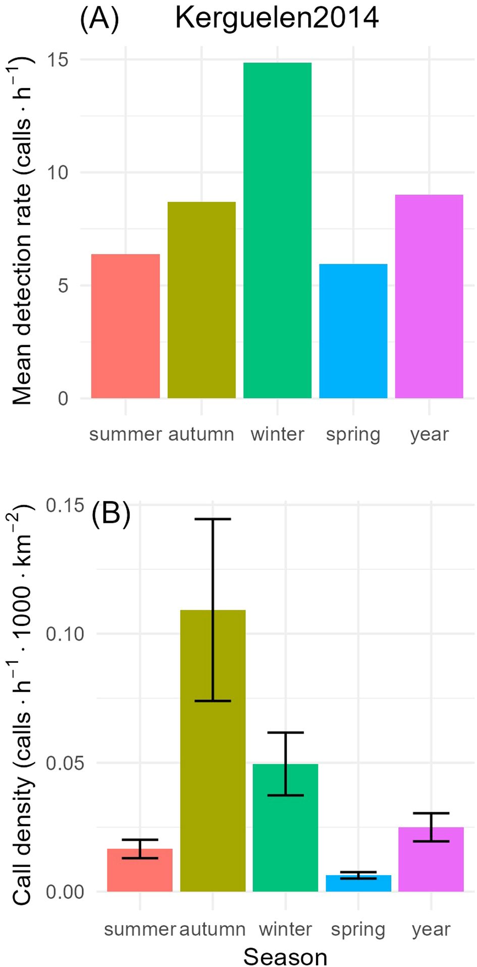
Figure 7. Top (A): mean detection rate (in units of calls/h) of Antarctic blue whale tonal calls at S. Kerguelen Plateau 2014 for each time period. Mean detection rates were calculated by dividing the total number of detections by the total duration of monitoring in each time period. Bottom (B): call densities (in units of calls/h/1000 km²) for each time period with error-bars showing the 95% confidence intervals for each time period.

Table 2

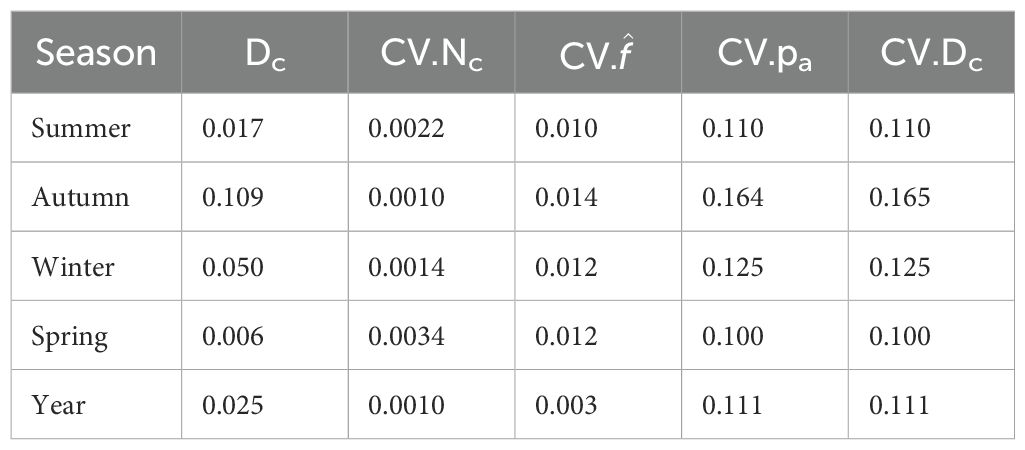
Table 2. Results of call density estimation for each season including: density of calls (D_c) in units of calls/h/1000 km², coefficient of variation for the parameters n_c, f, p_a, and D_c.

Detection rate peaked in winter at approximately 15 calls/h. In other seasons, these ranged from 5-8 calls/h (Figure 7). In contrast, maximum call densities occurred in autumn, followed by winter, and minimum call densities occurred in spring.

4 Discussion

4.1 Call density vs. detection rate

Here we present the first estimates of seasonal call densities of Antarctic blue whale song-calls from acoustic recordings made in the Antarctic. Previous passive acoustic studies of ABW calls in the Antarctic have focused on detection rate, and this has made it challenging to understand ecological and biological trends in detections over time and space. Our estimates of call density are more easily interpreted than estimates of detection rate – even if obtaining them is more complicated. By accounting for detection range and detector performance, we ensure that our call densities can be interpreted as some combination of animal density and animal behaviour – factors that are purely biological/ecological in nature. Detection rates, as they are usually presented, are simpler to estimate than call densities. However, within the detection rate the biological factors of interest are confounded with covariates from the physical environment (noise, propagation, detection range) and the detection process (detector performance). Accounting for variability in detection range and detector performance and propagating this variability throughout our call density estimate also provides a means of estimating the CV (and corresponding confidence intervals) of our seasonal call densities.

Plotting our seasonal call densities with confidence intervals reveals differences across seasons, without overlap in 95% confidence intervals. Furthermore, the seasonal pattern of call densities that we found was different from that of detection rate. Detection rate showed a maximum in the winter, with middling detection rates for summer, autumn, and spring that were all relatively indiscernible (within 2.5 in units of calls/h) from each other since they were confounded by greatly varying noise levels and thus ${\widehat{p}}_a$. Our call densities peaked at a maximum in autumn, falling to a clear minimum in spring. Thus, our data demonstrate that there is a quantifiable seasonal difference in call density, and that this difference was driven by some combination of seasonal changes in ABW density, and/or acoustic behaviour.

The apparent seasonal pattern in call density can serve, alongside other independently derived knowledge of blue whale life history, to develop and test further hypotheses about the biological function of these sounds. For example, it has long been hypothesized, with no evidence to the contrary, that blue whale song calls are produced by males (Oleson et al., 2007; Lewis et al., 2018), and are linked to breeding. Furthermore, there is some evidence from early studies that ABWs have a prolonged and temporally diffuse breeding season over autumn and winter, and that this correlates with a prolonged and temporally diffuse migration to lower latitudes in these seasons (Brown, 1954; Mackintosh, 1966). The seasonal pattern of call density from our high-latitude Southern Indian Ocean site in 2014 appears to be in accord with these facets of ABW life-history, whereas detection rates would at best be considered ambiguous or inconclusive for testing this hypothesis.

Our interpretation of our acoustic data is that the peak in call density in autumn corresponds to the start of the (relatively prolonged) breeding period. We suspect the second-highest call densities in winter correspond to a potential behavioural peak in calling. However, this behavioural peak has a lower call density because fewer animals are within the detection range of our Antarctic recording site, potentially because the site is heavily ice-covered during winter, and potentially because a large proportion of calling animals have already migrated to lower latitudes, beyond even the very large detection range afforded by lower winter noise levels. The lowest call densities in spring correspond to time periods when ABWs switch their behaviour from breeding (and calling) to returning to the Antarctic to feed, and this reduced calling behaviour combined with largest values for ${\widehat{p}}_a$, and high-detection range (due to reduced noise level from ice-covered seas, e.g. observed by Shabangu et al. (2020), and from reduction in the blue and fin whale choruses), results in a minimum call density at our Antarctic recording site. The higher call densities in summer would correspond to a time when most of the population have returned to the Antarctic feeding grounds and more are in proximity to our recording site. As the summer progresses into autumn and the breeding season approaches their energetic needs are met, and then some of the animals begin to alter their behaviour from feeding (and not calling much) back towards calling again. Further studies of seasonal calling behaviour, particularly estimates of the acoustic-cue rate (call production rate of an individual), and the proportion of individuals that are making calls, could serve to help test these hypotheses. Furthermore, collection of these data would provide for estimation of ABW (animal) density from our call densities.

4.2 Variability and confidence intervals

The CVs of our seasonal call densities ranged from 0.11 - 0.15. These are reasonable CV values and are lower compared to other methods of estimating abundance of Antarctic blue whales. For example, line-transect abundance estimates of ABWs reported by Branch and Butterworth (2001) from circumpolar sightings surveys ranged from 0.41- 0.52. However, the CVs from Branch and Butterworth were for estimates of global population abundance, whereas our CVs were for local call density where variability over a shorter time period and study area may be inherently reduced. Further, information on the relationship between call density and animal density (e.g., the Z call production rate of ABW, and the proportion of the ABW population that make Z calls) would be required to convert our call densities into animal densities. Previous studies have shown that the CV associated with such behavioural parameters can contribute the largest amount to an animal density CV (e.g., Harris et al., 2018). So, the relatively good CVs from our call density estimate could still increase by a large amount when scaling up the study area and time period to population abundance, and including the additional behavioural parameter(s) (see Fregosi et al., 2022, for another example).

Variability in ${\widehat{p}}_a$ appeared to be the overwhelmingly dominant driver of the overall CV for our call densities (Table 2). The CV of ${\widehat{p}}_a$ was driven by variability in NL, SL and TL, but predominantly by the distributions of SL. For our study, the same SL distribution was used across all seasons with a mean of 189 dB and standard deviation of 8 dB. The high variability in our SL distribution comes from a study that applied the sonar equation and modelled TL in a similar manner: i.e. using the software RAMGeo to model a deep water Antarctic environment similar to that of our site. The variability in SL thus includes both localisation error, and model mismatch including errors in TL. So as not to double count the uncertainty in TL, we assumed that it was already included amongst our highly variable SL. While variability in SL was the main driver of the CV of our call densities, the seasonal differences in our mean call densities were driven by noise.

Our distributions of NL showed substantial variability by season (Figure 5), with NL variation primarily linked to ice cover and chorusing. Autumn had the largest CV (of D_c and ${\widehat{p}}_a$), with the remaining seasons CVs relatively similar (within 0.02).

We chose shape constrained GAMs because our dataset produced GAMs that exhibited unrealistic behaviour at very high and low SNR without constraints. In future studies, it would be worth testing whether annotating a larger amount of data would improve the precision of our SNR-detection function, and subsequent estimates of CV of ${\widehat{p}}_a$ and of call density. This could be achieved in practice by adaptively annotating additional hours of summer recordings to supplement the distribution of summer SNR. Additionally, the spectrogram correlation detector that we used had poor recall for an acceptable level of precision, see (Miller et al., 2021a), so it would be worth exploring in a future study the extent to which using a better (i.e., less variable) detector could lower the CVs. The use of deep learning algorithms in conjunction with closed population capture-recapture models (Miller et al., 2022) has emerged as a novel approach to achieving improved results in call detection. Also, Schall et al. (2024), presented a deep learning benchmark for the detection of blue and fin whale vocalizations in marine long-term PAM dataset.

4.3 Further exploration and advancement of call density methods

The analysis that we presented here represents an initial first-step toward a standardized measure of bioacoustic detections of ABWs recorded on single instruments that is suitable for comparison across different timespans, in addition to sites. Future work can focus on transforming extant estimates of detection rates into call densities, but we also expect that there will be further modifications and hopefully improvements to the various steps that comprise this method. Such improvements and modifications might include: improved detectors with better recall, lower $\widehat{f}$, less variability in SNR-detection curves. A natural extension might also be to investigate call density over shorter time periods than annual & seasonal: e.g. monthly or weekly (though care has to be taken regarding sharing parameters between smaller time periods). Further, a key limitation of our method is that we have to assume a uniform call density across the area, thus it would be preferable to account for heterogeneity in spatial distribution of calls, if a priori knowledge is available (e.g., Harris et al., 2018). For example, in winter, large portions of our study area are covered by sea ice. Fully ice-covered areas may be less likely to contain whale calls than open water, so a simulation that included such effects of ice-cover and any other spatial covariates would be an important improvement.

Additionally, there is scope for improvement in estimation of TL, particularly via populating TL models with more accurate and higher-resolution environmental parameters, and accounting for uncertainty in model inputs where necessary. For example: higher-resolution and more accurate bathymetry than etopo1 could be used where available. Similarly, more accurate local SSPs than those derived from decadal & broad-spatial averages could also be used where available. Ideally, this would involve using in-situ data from argos floats and scientific surveys that occur in the vicinity of the monitoring sites (spatially and in time). Furthermore, it might also include modifications to vary the SSP spatially along each radial (in the same manner as bathymetry). And lastly, our assumption of homogenous seabed geoacoustics could be improved upon. In the Antarctic, little is known about density and sound-speed of the seabed at any location, but once measures are made at a location, these are likely to remain stable for a long time, so such data do have good potential for longevity/legacy, as well as retrospective re-analysis of call density should they become available. Such analysis would be important when comparing across different sites, but is less important for analyses comparing different time periods at a single site (like our seasonal analysis here) since these properties are not likely to vary much over time.

Compared to the potential improvements in estimating TL, there are fewer avenues for improvements in measuring NL. The main NL-related modification that would be useful to consider in future studies would be excluding times with very high noise from call density estimates. This would be analogous to going ‘off-effort,’ when conditions are unsuitable for detection, as is commonly done when estimating animal abundance with distance sampling. For example, during at-sea line-transect distance sampling surveys, visual observers stop data collection when the sightability is poor (e.g. sea-state is > Beaufort 5). This saves them time looking for animals in conditions where they would be very unlikely to detect anything, and costs little in the way of a reduction in number of detections. More importantly it also reduces variability of their density estimates. Applying this analogy to acoustics would involve identifying periods when high levels of noise prohibit reliable detection, and then excluding these periods from the estimates of call density.

Finally, there appears to be some scope to modify and improve upon estimation of SNR, detector characterisation, and false discovery rates. Estimation of SNR is an often overlooked and/or over-simplified aspect of passive acoustics, and so further investigation into how best to estimate SNR for call density estimation may be warranted. Questions for such investigation might include the timeframe over which to estimate noise and signal, and whether level measurements should focus on measures of central tendency (e.g. RMS, L50 measurements), or maxima (e.g. peak, L90). For the tonal calls of ABWs in this study the frequency band of interest was narrow and clearly defined, but for frequency-modulated calls, like blue whale D-calls it may not be appropriate to calculate signal and noise levels over a simple rectangular time-frequency box. Thus, there may be further need to better define the call in the time-frequency plane, e.g. by tracing a contour, for such calls. Another potential improvement related to SNR would be to better understand the effects of floating ground-truth on detector characterisation. For example, adjudicated mark-recapture methods, like those proposed by Miller et al. (2022), might be better able to address issues of variability and subjectivity in the human analysts annotations, and reduce potential biases that flow through to the SNR-detection function and $\widehat{f}$.

4.4 Implications for long-term monitoring (conclusions)

The methods that we have presented here represent a pathway to extract even more value from the increasingly large body of knowledge generated from worldwide long-term single sensor recordings of low-frequency baleen whales. These methods should be directly applicable not just to ABWs, but any subspecies or population of blue whales, fin whales. These methods potentially the low-frequency omnidirectional calls of minke, sei, and right whales, where other standard density estimation methods such as distance sampling and spatial-capture recapture cannot be applied. Further adaptations to the propagation modelling and source-level estimation could make these methods suitable for broadband calls of baleen whales, like humpback whales – similar to the methods proposed by Helble et al. (2013), and the Monte Carlo simulation method using odontocete clicks has been applied in several studies (Küsel et al., 2011; Hildebrand et al., 2015; Frasier et al., 2016).

For ABWs, application of this method across a wider geographic and temporal span of sites throughout the Southern Hemisphere would represent a pathway to deliver a cost-effective, statistically-robust, and intuitively-interpretable, long-term, global investigation of bioacoustic trends for this critically endangered subspecies. The method would be cost-effective since there have already been millions of hours of long-term underwater recordings that have been collected worldwide over the past two decades, and this sort of data is continuing to become more affordable to collect and analyse as technology progresses. The results of this method are statistically robust, with variability of each component propagated through to the final estimates of call density. But most importantly, the method produces results, call densities, that can be directly compared independent of the recording equipment, site-specific environmental factors, and detection methods, and that are driven by biological factors: animal density and behaviour.

As large-scale changes occur in the global ocean, these can have potential impacts on the distributions and abundance of pelagic prey and the whales species that feed upon it e.g (Moore, 2008; Moore and Huntington, 2008). Monitoring baleen whale call densities across large areas and timescales, including the use of existing passive acoustic datasets like those collected by the Southern Ocean Research Partnership (Opzeeland et al., 2013; Miller et al., 2021c), the Preparatory Commission for the Comprehensive Nuclear-Test-Ban Treaty Organization, or the Global Ocean Observing System, can be a valuable source of information for understanding the dynamics of changing pelagic ecosystems and is a step forward for global ocean observation.

Data availability statement

The raw data supporting the conclusions of this article will be made available by the authors, without undue reservation.

Ethics statement

Ethical approval was not required for the study involving animals in accordance with the local legislation and institutional requirements because the study was purely observational.

Author contributions

FC: Data curation, Formal analysis, Writing – original draft, Writing – review & editing. DH: Conceptualization, Funding acquisition, Methodology, Supervision, Writing – original draft, Writing – review & editing. SB: Conceptualization, Funding acquisition, Methodology, Supervision, Writing – original draft, Writing – review & editing, Project administration. NB: Writing – review & editing, Data curation. BM: Data curation, Writing – review & editing, Conceptualization, Formal analysis, Funding acquisition, Methodology, Supervision, Writing – original draft.

Funding

The author(s) declare financial support was received for the research, authorship, and/or publication of this article. This research was funded by International Whaling Commission-Southern Ocean Research Partnership (IWC-SORP) to SB (IWC SORP Research Fund Project 17). This research was also made possible by Australian Antarctic Division (AAD) AAS projects 4102 & 4600.

Acknowledgments

We thank the other members of the Acoustic Trends Working Group (Dr. Ana Širović, Dr. Fannie Shabangu, Dr. Flore Samaran, Dr. Ilse Van Opzeeland, Dr. Kathleen Stafford, and Dr. Ken Findlay) which is part of the Southern Ocean Research Partnership (SORP), for sharing their thoughts and supporting each step of this research development. BM thanks Drs Nat Kelly and Simon Wotherspoon from the AAD for their patience, guidance, and many conversations on distance sampling and density estimation. SB thanks the Center for Oceanographic Research COPAS COASTAL at the University of Concepción, Chile, funded by the Chilean Agencia Nacional de Investigación y Desarrollo (ANID) grant FB210021.

Conflict of interest

The authors declare that the research was conducted in the absence of any commercial or financial relationships that could be construed as a potential conflict of interest.

Publisher’s note

All claims expressed in this article are solely those of the authors and do not necessarily represent those of their affiliated organizations, or those of the publisher, the editors and the reviewers. Any product that may be evaluated in this article, or claim that may be made by its manufacturer, is not guaranteed or endorsed by the publisher.

References

Amante C., Eakins B. W. (2009). ETOPO1 1 Arc-Minute Global Relief Model: Procedures, Data Sources and Analysis. NOAA Technical Memorandum NESDIS NGDC-24 (National Geophysical Data Center, NOAA). doi: 10.7289/V5C8276M

Crossref Full Text | Google Scholar

Balcazar N. E., Tripovich J. S., Klinck H., Nieukirk S. L., Mellinger D. K., Dziak R. P., et al. (2015). Calls reveal population structure of blue whales across the southeast Indian Ocean and southwest Pacific Ocean. J. Mammalogy 96 (6), 1184-1193. doi: 10.1093/jmammal/gyv126

Crossref Full Text | Google Scholar

Borchers D. L., Buckland S. T., Zucchini W. (2002). Estimating Animal Abundance (London: Springer London). doi: 10.1007/978-1-4471-3708-5

Crossref Full Text | Google Scholar

Bouffaut L., Landrø M., Potter J. R. (2021). Source level and vocalizing depth estimation of two blue whale subspecies in the western Indian Ocean from single sensor observations. J. Acoustical Soc. America 149, 4422–4436. doi: 10.1121/10.0005281

Crossref Full Text | Google Scholar

Boyer T. P., Garcia H. E., Locarnini R. A., Zweng M. M., Mishonov A. V., Reagan J. R., et al. (2018). World Ocean Atlas 2018 (NOAA National Centers for Environmental Information). Available online at: https://accession.nodc.noaa.gov/NCEI-WOA18 (Accessed August 3, 2021).

Google Scholar

Branch T. A. (2007). Abundance of Antarctic blue whales south of 60 S from three complete circumpolar sets of surveys. J. Cetacean Res. Manage. 9, 253–262. Available at: http://www.iwcoffice.co.uk/_documents/sci_com/sc59docs/sc-59-SH9.pdf.

Google Scholar

Branch T. A., Butterworth D. S. (2001). Estimates of abundance south of 60° S for cetacean species sighted frequently on the 1978/79 to 1997/98 IWC/IDCR-SOWER sighting surveys. J. Cetacean Res. Manage. 3, 251–270. doi: 10.47536/jcrm.v3i3

Crossref Full Text | Google Scholar

Brown S. (1954). “Dispersal in blue and fin whales,” in Discovery Reports, vol. 26. , 357–384. Available at: http://scholar.google.com/scholar?hl=en&btnG=Search&q=intitle:Dispersal+in+blue+and+fin+whales#0.

Google Scholar

Cochran W. G. (1977). Sampling techniques (New York, USA: John Wiley & Sons).

Google Scholar

Collins M. D. (2002). User’s Guide for RAM Version 1.0 and 1.0p. Available online at: http://oalib.hlsresearch.com/AcousticsToolbox/. (accessed [August 7, 2024])

Google Scholar

Cooke J. G. (2018). Balaenoptera musculus ssp. intermedia (The IUCN Red List of Threatened Species), e.T41713A50226962. doi: 10.2305/IUCN.UK.2018-2.RLTS.T41713A50226962.en

Crossref Full Text | Google Scholar

Dréo R., Bouffaut L., Leroy E., Barruol G., Samaran F. (2019). Baleen whale distribution and seasonal occurrence revealed by an ocean bottom seismometer network in the Western Indian Ocean. Deep-Sea Res. Part II: Topical Stud. Oceanography 161, 132–144. doi: 10.1016/j.dsr2.2018.04.005

Crossref Full Text | Google Scholar

Duncan A. (2005). Acoustics Toolbox User interface and Post processor (AcTUP). Available online at: http://cmst.curtin.edu.au/products/underwater/. (accessed [August 7, 2024])

Google Scholar

Dutkiewicz A., Müller R. D., O’Callaghan S., Jónasson H. (2015). Census of seafloor sediments in the world’s ocean. Geology 43, 795–798. doi: 10.1130/G36883.1

Crossref Full Text | Google Scholar

Frasier K. E., Wiggins S. M., Harris D., Marques T. A., Thomas L., Hildebrand J. A. (2016). Delphinid echolocation click detection probability on near-seafloor sensors. J. Acoust. Soc Am. 140, 1918–1930. doi: 10.1121/1.4962279

PubMed Abstract | Crossref Full Text | Google Scholar

Fregosi S., Harris D. V., Matsumoto H., Mellinger D. K., Martin S. W., Matsuyama B., et al. (2022). Detection probability and density estimation of fin whales by a Seaglider. J. Acoustical Soc. America 152, 2277–2291. doi: 10.1121/10.0014793

Crossref Full Text | Google Scholar

Gavrilov A. N., McCauley R. D., Gedamke J. (2012). Steady inter and intra-annual decrease in the vocalization frequency of Antarctic blue whales. J. Acoustical Soc. America 131, 4476–4480. doi: 10.1121/1.4707425

Crossref Full Text | Google Scholar

Harris D., Matias L., Thomas L., Harwood J., Geissler W. H. (2013). Applying distance sampling to fin whale calls recorded by single seismic instruments in the northeast Atlantic. J. Acoustical Soc. America 134, 3522–3535. doi: 10.1121/1.4821207

Crossref Full Text | Google Scholar

Harris D. V., Clarke T., Heaney K., Mellinger D. K., Miles D., Thomas L. (2024, submitted). Estimating the detection probability of long-ranging baleen whale song using a single sensor: towards density estimation. J. Acoustical Soc. Am.

Google Scholar

Harris D. V., Miksis-Olds J. L., Vernon J. A., Thomas L. (2018). Fin whale density and distribution estimation using acoustic bearings derived from sparse arrays. J. Acoustical Soc. America 143 (5), 2980-2993. doi: 10.1121/1.5031111

Crossref Full Text | Google Scholar

Helble T. A. (2013). Site specific passive acoustic detection and densities of humpback whale calls off the coast of California. Thesis. UC San Diego, CA, USA.

Google Scholar

Helble T. A., D’Spain G. L., Campbell G. S., Hildebrand J. A. (2013). Calibrating passive acoustic monitoring: Correcting humpback whale call detections for site-specific and time-dependent environmental characteristics. J. Acoustical Soc. America 134, EL400–EL406. doi: 10.1121/1.4822319

Crossref Full Text | Google Scholar

Hildebrand J. A., Baumann-Pickering S., Frasier K. E., Trickey J. S., Merkens K. P., Wiggins S. M., et al. (2015). Passive acoustic monitoring of beaked whale densities in the Gulf of Mexico. Sci. Rep. 5, 16343. doi: 10.1038/srep16343

PubMed Abstract | Crossref Full Text | Google Scholar

Jensen F. B., Kuperman W. A., Porter M. B., Schmidt H. (2011). Computational Ocean Acoustics (New York, NY: Springer New York). doi: 10.1007/978-1-4419-8678-8

Crossref Full Text | Google Scholar

Küsel E. T., Mellinger D. K., Thomas L., Marques T. A., Moretti D., Ward J. (2011). Cetacean population density estimation from single fixed sensors using passive acoustics. J. Acoustical Soc. America 129, 3610–3622. doi: 10.1121/1.3583504

Crossref Full Text | Google Scholar

Leroy E. C., Samaran F., Bonnel J., Royer J. (2016). Seasonal and diel vocalization patterns of Antarctic blue whale (Balaenoptera musculus intermedia) in the Southern Indian Ocean: A multi-year and multi-site study. PloS One 11, e0163587. doi: 10.1371/journal.pone.0163587

PubMed Abstract | Crossref Full Text | Google Scholar

Letsheleha I. S., Shabangu F. W., Farrell D., Andrew R. K., la Grange P. L., Findlay K. P. (2022). Year-round acoustic monitoring of Antarctic blue and fin whales in relation to environmental conditions off the west coast of South Africa. Mar. Biol. 169, 41. doi: 10.1007/s00227-022-04026-x

Crossref Full Text | Google Scholar

Lewis L. A., Calambokidis J., Stimpert A. K., Fahlbusch J., Friedlaender A. S., McKenna M. F., et al. (2018). Context-dependent variability in blue whale acoustic behaviour. R. Soc. Open Sci. 5 (8), 180241. doi: 10.1098/rsos.180241

PubMed Abstract | Crossref Full Text | Google Scholar

Ljungblad D. K., Clark C. W., Shimada H. (1998). A comparison of sounds attributed to pygmy blue whales (Balaenoptera musculus brevicauda) recorded south of the Madagascar Plateau and those attributed to ‘true’ blue whales (Balaenoptera musculus) recorded of Antarctica. Rep. Int. Whaling Commission 48, 439–442.

Google Scholar

Lurton X. (2010). An Introduction to Underwater Acoustics: Principles and Applications (London ; New York: Springer Science & Business Media).

Google Scholar

Mackintosh N. A. (1966). “The distribution of southern blue and fin whales,” in Whales, dolphins and porpoises. Ed. Norris K. S. (University of California Press, Berkeley and Los Angeles), 125–145.

Google Scholar

Marques T. A., Thomas L., Martin S. W., Mellinger D. K., Ward J. A., Moretti D. J., et al. (2013). Estimating animal population density using passive acoustics. Biol. Rev. 88, 287–309. doi: 10.1111/brv.12001

Crossref Full Text | Google Scholar

McCauley R. D., Jenner C., Bannister J. L., Burton C. L. K., Cato D. H., Duncan A. (2001). Blue whale calling in the Rottnest Trench – 2000, western Australia. Report R2001-6, Centre for Marine Science and Technology, Curtin University of Technology, Perth, Western Australia.

Google Scholar

McDonald M. A., Fox C. G.. (1999). Passive acoustic methods applied to fin whale population density estimation. J. Acoustical Soc. Am 105, 2643–2651.

Google Scholar

Mellinger D. K., Stafford K. M., Moore S. E., Dziak R. P., Matsumoto H. (2007). An overview of fixed passive acoustic observation methods for cetaceans. Oceanography 20, 36–45. doi: 10.1109/PASSIVE.2008.4786981

Crossref Full Text | Google Scholar

Menze S., Zitterbart D. P., van Opzeeland I., Boebel O. (2017). The influence of sea ice, wind speed and marine mammals on Southern Ocean ambient sound. R. Soc. Open Sci. 4, 160370. doi: 10.1098/rsos.160370

PubMed Abstract | Crossref Full Text | Google Scholar

Miksis-Olds J. L., Harris D. V., Mouw C. (2019). Interpreting fin whale (balaenoptera physalus) call behavior in the context of environmental conditions. Aquat. Mammals 45, 691–705. doi: 10.1578/AM.45.6.2019.691

Crossref Full Text | Google Scholar

Miller B. S., Balcazar N., Nieukirk S., Leroy E. C., Aulich M., Shabangu F. W., et al. (2021a). An open access dataset for developing automated detectors of Antarctic baleen whale sounds and performance evaluation of two commonly used detectors. Sci. Rep. 11, 806. doi: 10.1038/s41598-020-78995-8

PubMed Abstract | Crossref Full Text | Google Scholar

Miller B. S., Barlow J., Calderan S., Collins K., Leaper R., Olson P., et al. (2015). Validating the reliability of passive acoustic localisation: a novel method for encountering rare and remote Antarctic blue whales. Endangered Species Res. 26, 257–269. doi: 10.3354/esr00642

Crossref Full Text | Google Scholar

Miller B. S., Calderan S., Leaper R., Miller E. J., Širović A., Stafford K. M., et al. (2021b). Source level of antarctic blue and fin whale sounds recorded on sonobuoys deployed in the deep-ocean off Antarctica. Front. Mar. Sci. 8. doi: 10.3389/fmars.2021.792651

Crossref Full Text | Google Scholar

Miller B. S., Calderan S., Miller E. J., Širović A., Stafford K. M., Bell E., et al. (2019). “A passive acoustic survey for marine mammals conducted during the 2019 Antarctic voyage on Euphausiids and Nutrient Recycling in Cetacean Hotspots (ENRICH),” in Proceedings of ACOUSTICS 2019, Cape Schanck, Victoria, Australia: Australian Acoustical Society. 1–10.

Google Scholar

Miller B. S., Madhusudhana S., Aulich M. G., Kelly N. (2022). Deep learning algorithm outperforms experienced human observer at detection of blue whale D‐calls: a double‐observer analysis. Remote Sens Ecol. Conserv. 9 (1), 104-116. doi: 10.1002/rse2.297

Crossref Full Text | Google Scholar

Miller B. S., Miller E., Calderan S., Leaper R., Stafford K., Širović A., et al. (2017). “Circumpolar acoustic mapping of endangered Southern Ocean whales: Voyage report and preliminary results for the 2016/17 Antarctic Circumnavigation Expedition,” in Paper SC/67a/SH03 submitted to the Scientific Committee 67a of the International Whaling Commision, Bled Slovenia, Vol. 18.

Google Scholar

Miller B. S., Milnes M., Whiteside S. (2021c). Long-term underwater acoustic recordings 2013-2019. Ver. 4. doi: 10.26179/h7xa-y729

Crossref Full Text | Google Scholar

Miller B. S., Milnes M., Whiteside S., Double M. C., Gedamke J. (2016). “Calibrated underwater sound levels at two Antarctic recording sites : the seasonality of sounds from wind, ice, and marine mammals,” in Paper submitted to the Scientific Committee of the International Whaling Commission. SC66B. Bled, Slovenia. SC/66B/SH19. 1–13.

Google Scholar

Miller B. S., Stafford K. M., Van Opzeeland I., Harris D., Samaran F., Širović A., et al. (2020). An annotated library of underwater acoustic recordings for testing and training automated algorithms for detecting Antarctic blue and fin whale sounds. doi: 10.26179/5e6056035c01b. (Accessed [August 7, 2024])

Crossref Full Text | Google Scholar

Moore S. E. (2008). Marine mammals as ecosystem sentinels. J. Mammalogy 89, 534–540. doi: 10.1644/07-MAMM-S-312R1.1

Crossref Full Text | Google Scholar

Moore S. E., Huntington H. P. (2008). Arctic marine mammals and climate change: impacts and resilience. Ecol. Appl. 18, S157–S165. doi: 10.1890/06-0571.1

PubMed Abstract | Crossref Full Text | Google Scholar

Nghiem‐Phu L., Tappert F. (1985). Modeling of reciprocity in the time domain using the parabolic equation method. J. Acoustical Soc. America 78, 164–171. doi: 10.1121/1.392553

Crossref Full Text | Google Scholar

Oedekoven C. S., Marques T. A., Harris D., Thomas L., Thode A. M., Blackwell S. B., et al (2021). A comparison of three methods for estimating call densities of migrating bowhead whales using passive acoustic monitoring. Environ. Ecol. Statistics. doi: 10.1007/s10651-021-00506-3

Crossref Full Text | Google Scholar

Oleson E. M., Calambokidis J., Burgess W. C., McDonald M. A., LeDuc C. A., Hildebrand J. A. (2007). Behavioral context of call production by eastern North Pacific blue whales. Mar. Ecol. Prog. Ser. 330, 269–284. Available at: http://escholarship.org/uc/item/5xk9k7bp.pdf.

Google Scholar

Opzeeland I. V., Samaran F., Stafford K., Findlay K., Gedamke J., Harris D., et al. (2013). Towards collective circum-Antarctic passive acoustic monitoring: The Southern Ocean Hydrophone Network (SOHN). Polarforschung 83, 47–61.

Google Scholar

Payne R., Webb D. (1971). Orientation by means of long range acoustic signaling in baleen whales. Ann. New York Acad. Sci. 188, 110–141. doi: 10.1111/j.1749-6632.1971.tb13093.x

Crossref Full Text | Google Scholar

Porter M. B. (2020). Acoustics Toolbox. Acoustics Toolbox. Available online at: http://oalib.hlsresearch.com/AcousticsToolbox/ (Accessed August 2, 2021).

Google Scholar

Pya N. (2022). scam: Shape Constrained Additive Models. Available online at: https://CRAN.R-project.org/package=scam. (accessed [August 7, 2024])

Google Scholar

Rankin S., Ljungblad D. K., Clark C. W., Kato H. (2005). Vocalisations of Antarctic blue whales, Balaenoptera musculus intermedia, recorded during the 2001/2002 and 2002/2003 IWC/SOWER circumpolar cruises, Area V, Antarctica. J. Cetacean Res. And Manage. 7, 13–20. doi: 10.47536/jcrm.v7i1

Crossref Full Text | Google Scholar

R Core Team (2019). R: A language and environment for statistical computing. Available online at: https://www.r-project.org/. (accessed [August 7, 2024])

Google Scholar

Rocha J. R.C., Clapham P. J., Ivashchenko Y. (2015). Emptying the oceans: A summary of industrial whaling catches in the 20th century. Mar. Fisheries Rev. 76, 37–48. doi: 10.7755/MFR

Crossref Full Text | Google Scholar

Samaran F., Adam O., Guinet C. (2010a). Detection range modeling of blue whale calls in Southwestern Indian Ocean. Appl. Acoustics 71, 1099–1106. doi: 10.1016/j.apacoust.2010.05.014

Crossref Full Text | Google Scholar

Samaran F., Guinet C., Adam O., Motsch J.-F., Cansi Y. (2010b). Source level estimation of two blue whale subspecies in southwestern Indian Ocean. J. Acoustical Soc. America 127, 3800–3808. doi: 10.1121/1.3409479

Crossref Full Text | Google Scholar

Samaran F., Stafford K. M., Branch T. A., Gedamke J., Royer J.-Y., Dziak R. P., et al. (2013). Seasonal and geographic variation of Southern blue whale subspecies in the Indian Ocean. PloS One 8, e71561. doi: 10.1371/journal.pone.0071561

PubMed Abstract | Crossref Full Text | Google Scholar

Schall E., Kaya I. I., Debusschere E., Devos P., Parcerisas C. (2024). Deep learning in marine bioacoustics: a benchmark for baleen whale detection. Remote Sensing in Ecology and Conservationdoi: 10.1002/rse2.392

Crossref Full Text | Google Scholar

Seber G. (1982). The estimation of animal abundance and related parameters. Macmillan, New York, USA.

Google Scholar

Shabangu F., Andrew R., Yemane D., Findlay K. (2020). Acoustic seasonality, behaviour and detection ranges of Antarctic blue and fin whales under different sea ice conditions off Antarctica. Endangered Species Res. 43, 21–37. doi: 10.3354/esr01050

Crossref Full Text | Google Scholar

Shabangu F. W., Findlay K. P., Yemane D., Stafford K. M., van den Berg M., Blows B., et al. (2019). Seasonal occurrence and diel calling behaviour of Antarctic blue whales and fin whales in relation to environmental conditions off the west coast of South Africa. J. Mar. Syst. 190, 25–39. doi: 10.1016/j.jmarsys.2018.11.002

Crossref Full Text | Google Scholar

Shabangu F. W., Yemane D., Stafford K. M., Ensor P., Findlay K. P. (2017). Modelling the effects of environmental conditions on the acoustic occurrence and behaviour of Antarctic blue whales. PloS One 12, e0172705. doi: 10.1371/journal.pone.0172705

PubMed Abstract | Crossref Full Text | Google Scholar

Širović A., Hildebrand J. A. (2011). Using passive acoustics to model blue whale habitat off the Western Antarctic Peninsula. Deep Sea Res. Part II: Topical Stud. Oceanography 58, 1719–1728. doi: 10.1016/j.dsr2.2010.08.019

Crossref Full Text | Google Scholar

Širović A., Hildebrand J. A., Wiggins S. M. (2007). Blue and fin whale call source levels and propagation range in the Southern Ocean. J. Acoustical Soc. America 122, 1208–1215. doi: 10.1121/1.2749452

Crossref Full Text | Google Scholar

Širović A., Hildebrand J. A., Wiggins S. M., McDonald M. A., Moore S. E., Thiele D. (2004). Seasonality of blue and fin whale calls and the influence of sea ice in the Western Antarctic Peninsula. Deep Sea Res. Part II: Topical Stud. Oceanography 51, 2327–2344. doi: 10.1016/j.dsr2.2004.08.005

Crossref Full Text | Google Scholar

Širović A., Hildebrand J. A., Wiggins S. M., Thiele D. (2009). Blue and fin whale acoustic presence around Antarctica during 2003 and 2004. Mar. Mammal Sci. 25, 125–136. doi: 10.1111/j.1748-7692.2008.00239.x

Crossref Full Text | Google Scholar

Thomas L., Marques T. (2012). Passive acoustic monitoring for estimating animal density. Acoustics Today 8, 35–44. Available at: http://link.aip.org/link/?ATCODK/8/35/1.

Google Scholar

Thomisch K. (2017). Distribution patterns and migratory behavior of Antarctic blue whales (Bremerhaven, Germany: Alfred-Wegener-Institut Helmholtz-Zentrum für Polar- und Meeresforschung Am). doi: 10.2312/BzPM_0707_2017

Crossref Full Text | Google Scholar

Tripovich J. S., Klinck H., Nieukirk S. L., Adams T., Mellinger D. K., Balcazar N. E., et al. (2015). Temporal segregation of the Australian and Antarctic blue whale call types (Balaenoptera musculus spp.). J. Mammalogy 96 (3), 603-610. doi: 10.1093/jmammal/gyv065

Crossref Full Text | Google Scholar

Van Parijs S., Clark C. W., Sousa-Lima R. S., Parks S. E., Rankin S., Risch D., et al. (2009). Management and research applications of real-time and archival passive acoustic sensors over varying temporal and spatial scales. Mar. Ecol. Prog. Ser. 395, 21–36. doi: 10.3354/meps08123

Crossref Full Text | Google Scholar

Warren V. E., Širović A., McPherson C., Goetz K. T., Radford C. A., Constantine R. (2021). Passive acoustic monitoring reveals spatio-temporal distributions of Antarctic and pygmy blue whales around central New Zealand. Front. Mar. Sci. 7. doi: 10.3389/fmars.2020.575257

Crossref Full Text | Google Scholar

Wilcock W. S. D. (2012). Tracking fin whales in the northeast Pacific Ocean with a seafloor seismic network. J. Acoustical Soc. America 132, 2408–2419. doi: 10.1121/1.4747017

Crossref Full Text | Google Scholar

Yun S., Lee W. S., Dziak R. P., Roche L., Matsumoto H., Lau T.-K., et al. (2021). Quantifying soundscapes in the Ross sea, Antarctica using long-term autonomous hydroacoustic monitoring systems. Front. Mar. Sci. 8. doi: 10.3389/fmars.2021.703411

Crossref Full Text | Google Scholar