 William Copeland
 Penelope Wagner
 Nick Hughes
 Alistair Everett
 Trond Robertsen
- Værvarslinga divisjon for Nord-Norge, Norwegian Meteorological Institute, Tromsø, Norway
The MET Norway Ice Service (NIS) celebrated its fiftieth year as a formal operational sea ice information provider in 2020. Prior to the 1970’s, support to navigation had started off with ad-hoc observations from coastal stations on Svalbard in the 1930’s, before developing as a research programme in the 1960’s. Activity in the region has steadily increased, and now the NIS also supports a large number of research, tourist, and resource exploration vessels, in addition to the ice chart archive being a resource for climate change research. The Ice Service has always been at the forefront in the use of satellite Earth Observation technologies, beginning with the routine use of optical thermal infrared imagery from NASA TIROS and becoming a large user of Canadian RADARSAT-2 Synthetic Aperture Radar (SAR), and then European Copernicus Sentinel-1, in the 2000’s and 2010’s. Initially ice charts were a weekly compilation of ice information using cloud-free satellite coverage, aerial reconnaissance, and in situ observations, drawn on paper at the offices of the Norwegian Meteorological Institute (MET Norway) in Oslo. From 1997 production moved to the Tromsø office using computer-based Geographical Information System (GIS) software and the NIS developed the ice charting system Bifrost. This allowed the frequency of production to be increased to every weekday, with a greater focus on detailed sea ice concentrations along the ice edge and coastal zones in Eastern Greenland and in the Svalbard fjords. From 2010, the NIS has also provided a weekly austral summer ice chart for the Weddell Sea and Antarctic Peninsula. To further develop its capabilities, NIS engages in a number of national and international research projects and led the EU Horizon 2020 project, Key Environmental monitoring for Polar Latitudes and European Readiness (KEPLER). This paper summarises the overall mandate and history of the NIS, and its current activities including the current state of routine production of operational ice charts at the NIS for maritime safety in both the Arctic and Antarctic, and future development plans.
1 Introduction
The main aim of this paper is to give an overview of the activities of the MET Norway Ice Service (NIS) at the Norwegian Meteorological Institute (MET Norway) and address the current limitations and future prospects for the NIS in a changing Arctic. Not only will this serve as a historical record, but it will also aid our end users to better understand our products and processing chains.
1.1 Arctic navigation: challenges and opportunities
The Arctic Ocean is a nearly landlocked ocean consisting of two deep central basins, i.e. Eurasian and Amerasian, bordered by seven epicontinental seas, i.e. The Greenland Sea, Lincoln Sea, Beaufort Sea, Chukchi Sea, East Siberian Sea, Laptev Sea, Kara Sea and Barents Sea Jakobsson et al., 2003, 2012). The presence of multiyear sea ice coverage is consistent throughout the year in the northern Canadian and northern Fram Strait regions, although this is rapidly decreasing due to climate change (Massonnet et al., 2012; Babb et al., 2022; Regan et al., 2023). The presence of ice is not restricted to only Arctic latitudes, forming during the winter season within the Okhotsk, Baltic, Bering, Labrador Seas and Baffin and Hudson Bay, with significant inter annual variability (Serreze and Meier, 2018; Matveeva and Semenov, 2022). It is in regions with seasonal sea ice where reliable charting is of most interest, due to a combination of active year round maritime traffic and in some areas a very dynamic ice pack/ice edge (Babb et al., 2021). Despite declining sea ice, the trend is not spatially uniform, meaning regional trends can be masked by a pan Arctic approach (Onarheim and Årthun, 2017; Arthun et al., 2021).
Shipping in ice infested waters around the Arctic consists of a variety of maritime operators. These include, but are not limited to, fisheries, research, tourism, military, energy exploration and production, and cargo transport (Wagner et al., 2020). Calving glaciers and the creation of icebergs along the coasts of Svalbard and Greenland are an additional hazard, especially those icebergs that drift into the highly frequented waters of the Barents Sea, where they are particularly hazardous due to their small size (Løset and Carstens, 1996; Nesterov et al., 2023). This makes them difficult to detect. It was the sinking of the RMS Titanic in 1912 in the waters off of Newfoundland which was the catalyst for the International Convention for the Safety Of Life At Sea (SOLAS), which still governs maritime safety today International Maritime Organization, 1974, and resulted in the formation of the International Ice Patrol (IIP) (Murphy and Cass, 2012).
Climate change has caused a significant decline in the Arctic ice cover, resulting in more open water and increased accessibility to Arctic regions for maritime traffic and geopolitical purposes (Huntington et al., 2021; Meier and Stroeve, 2022). Over the last 4 decades, sea ice extent has decreased 40% in September and 10% in March (Meleshko et al., 2020). However, it is important to consider interannual variability when discussing operational sea ice forecasting, as such fluctuations in ice cover can pose a significant risk to maritime users (Mioduszewski et al., 2019; Stocker et al., 2020). The reduction of sea-ice thickness and extent does not translate to decreased risk of ice hazard along maritime routes, rather this results in an increased risk due to drift of residual multiyear ice embedded within the seasonal sea ice cover, which is difficult to detect both in satellite images and on shipboard radar. This is exemplified by the large inter-annual variability in open navigation days along the Northern Sea Route (NSR), with a marked increase from 2016 to an 88 day opening in 2020, followed by a drastic reduction to 0 in 2021 (CHNL, 2020). Consequently, a number of vessels became trapped, necessitating a protracted rescue period of multiple vessels over 2–3 months (Müller et al., 2023). Meanwhile on the North West Passage an increase in maritime traffic is observed due to the decrease in overall sea ice year on year. However, increasingly thinning multiyear ice drifting south onto the route through the summer, and an increase in lower ice class vessels operating in the region, has increased navigational risk (Dawson et al., 2022).
It’s also important to note that the term “ice free” when referring to the Arctic is a misnomer, because ice-free includes < 1 million km2 of sea ice (Kim et al., 2023) The term “ice free” is defined by a threshold for sea-ice extent, which indicates the area of ocean with at least 15 percent sea-ice concentration, as measured by the assimilation passive microwave sensor used by climate modellers (Overland and Wang, 2013). This terminology originated due to the limitation of models to assimilate sea ice data accurately, yet conflicts with the definition in the Sea Ice, 2014 Sea Ice Nomenclature. Due to the models being limited by this constraint, the risk to maritime activities increases significantly when the sea ice extent falls below this limit with ice that does not appear in the forecasts moving rapidly in regional areas. The increased outflow of multiyear ice through the Fram Strait and a propensity for more highly dynamic first year ice in the Barents sea and around Svalbard, raises the risks of navigational hazards in these regions.
Furthermore, tourism is opening up a wide variety of route possibilities, with summer cruises to the North Pole, and more daring expeditions into remote areas where there is a lack of historical in situ sea ice data. Over the last decade ship traffic across the Arctic has doubled, with the most significant increase observed in the Svalbard region (Stocker et al., 2020). Increased traffic opens up not only issues with regards to maritime safety, but also involves geopolitical tensions and ecological impacts for the region (Marchenko et al., 2015; Hovelsrud et al., 2023).
1.2 A brief history of the Norwegian Ice Service
Ice charting of the ice edge has been of particular interest to mariners since the beginning of the hunting industry in the Atlantic sector of the high Arctic during the mid 16th Century (Divine and Dick, 2006; Mö et al., 2020). The NIS has a partial ice observation catalogue spanning back to the 1500s created by the manual digitizing of early observations from ship logbooks and other records up to 2002, concluding with a collection of over 6000 charts, that can be viewed using GIS software (ACSYS, 2003). Sea ice observation and reporting grew in importance especially during the era of polar exploration, when sea ice conditions played a role in some of the most well-known expeditions led by the likes of the Norwegian explorers Fridthjof Nansen and Roald Amundsen. Svalbard became part of Norwegian territory in 1925, and from 1933 official sea ice bulletins were released from the newly built Isfjord Radio on Svalbard by the Norwegian Svalbard and Arctic Ocean Survey (NSIU) headed by Adolf Hoel. Hoel, a Norwegian polar region scientist, political activist and trade/industry promoter, led multiple expeditions to Svalbard and Greenland (Hoel, 1929; Drivenes, 1994). Reporting of sea ice continued right up until the beginning of World War Two, when operations temporarily ceased. In 1948, the NSIU was renamed to the Norwegian Polar Institute (NPI) as a result of post war structural change, and as of 1963, sea ice reporting started anew, led by the NPI from both Bjørnøya and Isfjord Radio.
In 1969 the meteorological institute in Oslo began to download NASA Television Infrared Observation Satellite (TIROS) analogue thermal infrared (TIR) satellite imagery, and in 1970 the NIS was formed.
Reporting from the stations Bjørnøya and Hopen were fairly routine and sent to the Meteorological Institute in Oslo for analysis in the early days of satellite imagery (Figures 1A-C). Satellite imagery allowed for a greater overview of the region, and approximate ice edge position data was sent from the meteorological institute to the stations during the 1970s. In addition to this there were ad hoc ice observation flights along the ice edge from Andøya to Svalbard. Ice edge locations were plotted, along with identification of icebergs as show in Figures 1D, E. If visibility was greatly reduced, the flight radar was used to calculate the rough position of the ice edge.
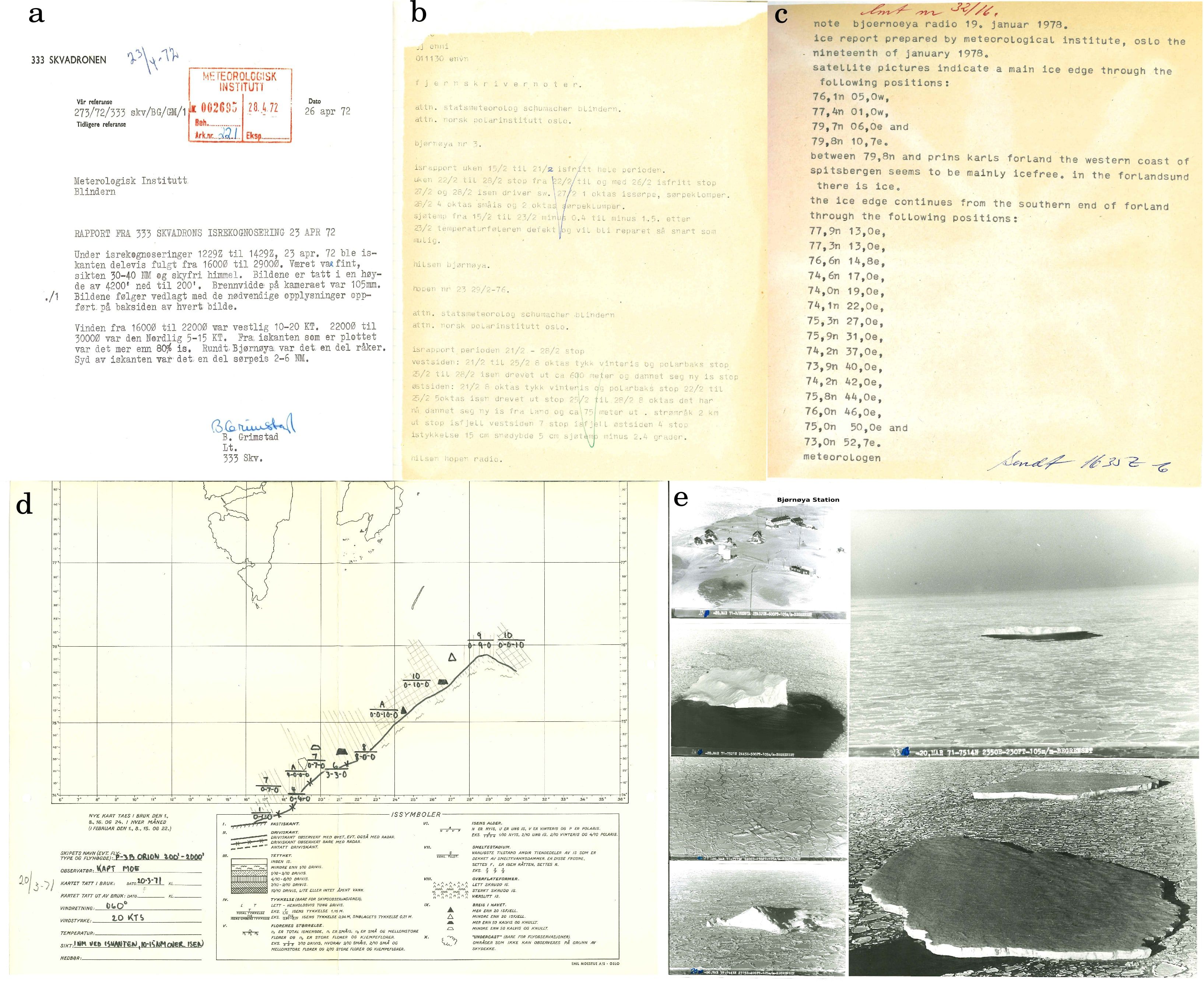
Figure 1. (A) Flight report from flyover 23rd April 1972, (B) Ice observations from Bjørnøya and Hopen sent to the Meteorological Institute February 1976, (C) Ice edge positions sent out from the meteorological institute using TIROS satellite imagery as a guide, (D) Ice edge plot map with icebergs from a flyover on 20th March 1971, (E) Aerial photographs complementing the plotting map for the same date as panel (D).
Today the NIS is the mandated authority for provision of sea ice and iceberg information in WMO/IOC JCOMM GMDSS METAREA-XIX. The service is also tied to the SOLAS convention, which has the main aim to ensure the safety of life and property at sea, designated by the International Maritime Organization (IMO) and the International Hydrographic Organization (IHO). To fulfil this mandate, the NIS provides standardised sea ice and weather information, forecasts and warnings. This includes daily (working day, Monday-Friday) ice concentration charts with an emphasis on Svalbard, the Barents Sea and eastern Greenland. The NIS also provides a weekly (on Mondays) ice chart for the Weddell and Bellingshausen Seas of the Antarctic during the austral summer (October to April) as part of the “Collaborative Antarctic Char” project between Norway, Russia and the United States. Several short-term sea ice forecast models are being evaluated on a pre-operational basis to assess their suitability for use in the Ice Service. These include: (a) U.S. Naval Research Laboratory GOF3.1 (Metzger et al., 2017), (b) Copernicus Marine Service (CMEMS) neXtSIM (Williams et al., 2021), and (c) the MET Norway Barents Ensemble Prediction System (Barents-EPS) model (Röhrs et al., 2023).
2 Area of study
2.1 METAREA XIX
The NIS provides ice charts for METAREA-XIX, covering the northern Norwegian mainland coastline, a large portion of the Greenland Sea, and the western Barents Sea, and the sector of the Arctic Ocean north of these areas up to the North Pole (see Figure 2) The ice charts include the entirety of this region with extension to include the entire Barents Sea, northern Baltic Sea, and the southern Greenland Sea, including the Denmark Strait. Ice charts also cover the Skagerrak, Kattegat and Outer-Oslofjord which can become ice covered in severe winters. The Svalbard region is the primary area of operations due to high ship traffic and where many of our end users operate.
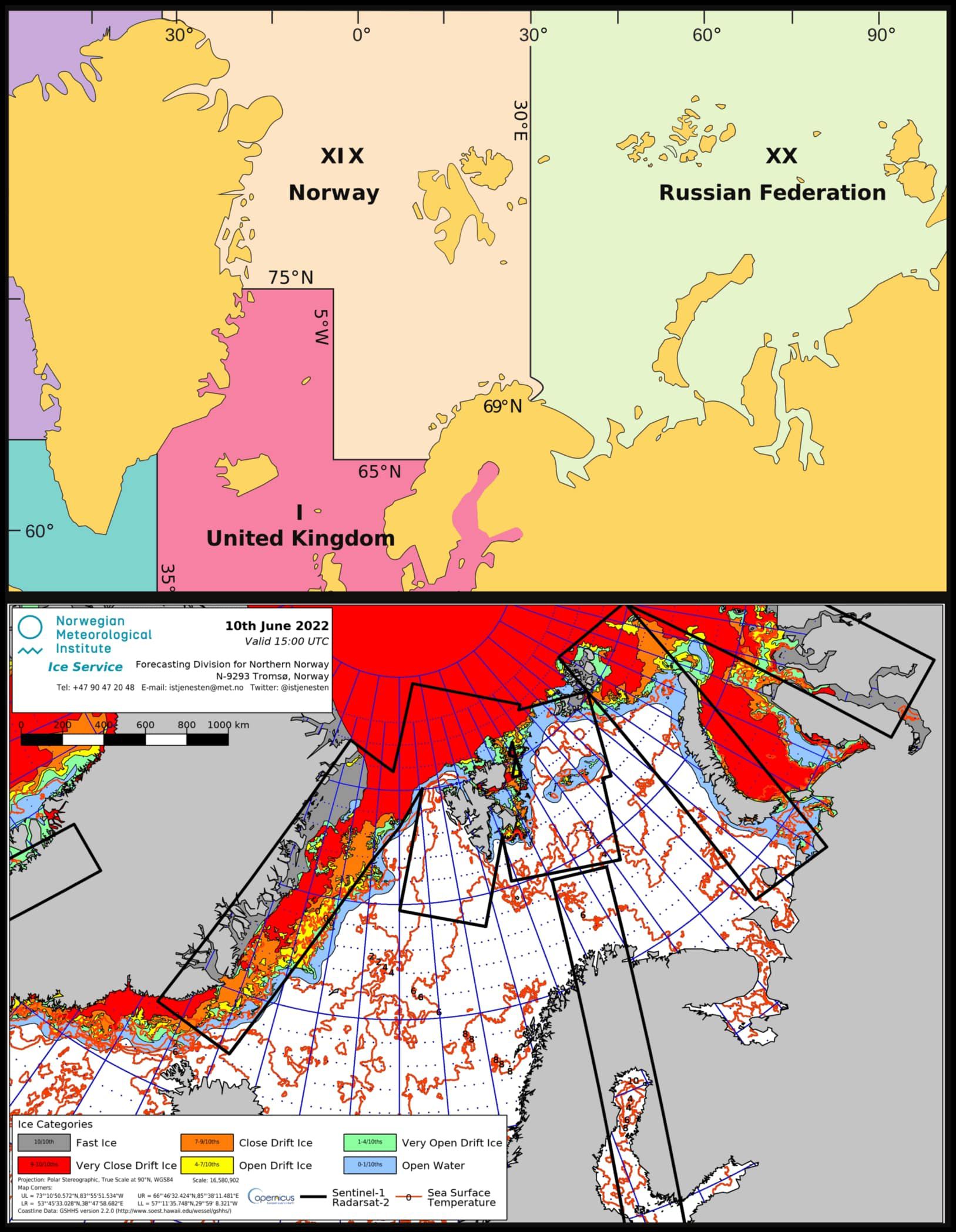
Figure 2. METAREA XIX along with the boundary area for NIS ice charts. Highest priority is given to the mandated area of the NIS, however maps are produced for further afield to complement ice charts created by other ice services e.g. AARI and Greenland ice service. Black boxes in the ice chart highlight available Sentinel 1 SAR imagery for the specific date.
European Arctic users of ice information are diverse, ranging from land communities, maritime navigators on leisure crafts to expert ice pilots. The foundations of user needs in METAREA XIX began with the fishing and hunting industry but quickly evolved to include tourism, the offshore energy sector, research expeditions, military activities, search-and-rescue (SaR) and general navigational vessels. Tourism is becoming a significant user base in this region, fuelled by a combination of increasing adventure tourism demand and increased duration of accessibility during the shoulder seasons (Stocker et al., 2020; Müller et al., 2023). The varying experience amongst ice pilots and increasingly dynamic ice conditions in this region during the shoulder months, raises the possibility of dangerous maritime incidents (Parsons and Progoulaki, 2014). The Svalbard and Barents region have especially dynamic ice conditions, arguably the greatest in the entire Arctic (Koenigk et al., 2008; Docquier et al., 2020).
During the Spring and Summer seasons the European Arctic experiences its highest vessel traffic, coinciding with sea ice retreat and rapidly changing ice movement. During this time, non-ice reinforced vessels are able to travel along and within the marginal ice zone (MIZ) and ice edge because the ice is often of low concentration. This allows for ships to travel to areas (i.e. fjords and narrow channels) that are normally inaccessible during the freeze-up and winter seasons. Meanwhile within the pack ice north of Svalbard, and more especially North East Greenland, first (FYI), second (SYI) and multiyear ice (MYI) cover presents itself with thick ridging, multi-year ice floes and potential for embedded icebergs throughout the year (Renner et al., 2013; Krumpen et al., 2016). Although this is changing as a result of climate change, with thinner ice becoming more predominant (Sumata et al., 2023), this environment continues to pose significant safety risks for the inexperienced and unprepared, especially those that do not fall under the goal-based polar code requirements (Müller et al., 2023).
One of the most challenging aspects for predicting sea ice conditions in METAREA XIX is inter-annual variability of sea ice in the region. This poses major challenges for long term route planning and predictability of the ice edge on a seasonal basis, that has traditionally relied upon climate based monitoring capabilities. Weather, and more especially sustained wind direction, plays a major role in changing sea ice extent, where thinner ice is more susceptible to wind and wave action. With a lack of in situ meteorological observational data in the Arctic region, models struggle to predict weather systems as comprehensively as they do in temperate and equatorial regions (Jung et al., 2016). This compounds the issues surrounding long term route planning for ships, especially tourist vessels that use the ice edge as their primary target, as forecasting resources and capabilities are greatly hindered.
2.2 The Antarctic
Although the mandate of the NIS does not extend to the Antarctic region, the NIS actively participates in the “Collaborative Antarctic Chart” project between Norway, Russia and the United States. During the austral summer, from the beginning of October to the end of April, weekly charts for the Weddell Sea and Antarctic Peninsula region are created every Monday, aligning with the summer tourist season in the region (Figure 3). Most importantly, the NIS contributes to the Antarctic Iceberg Database, with naming supplemented by the U.S. National Ice Center, 2024.
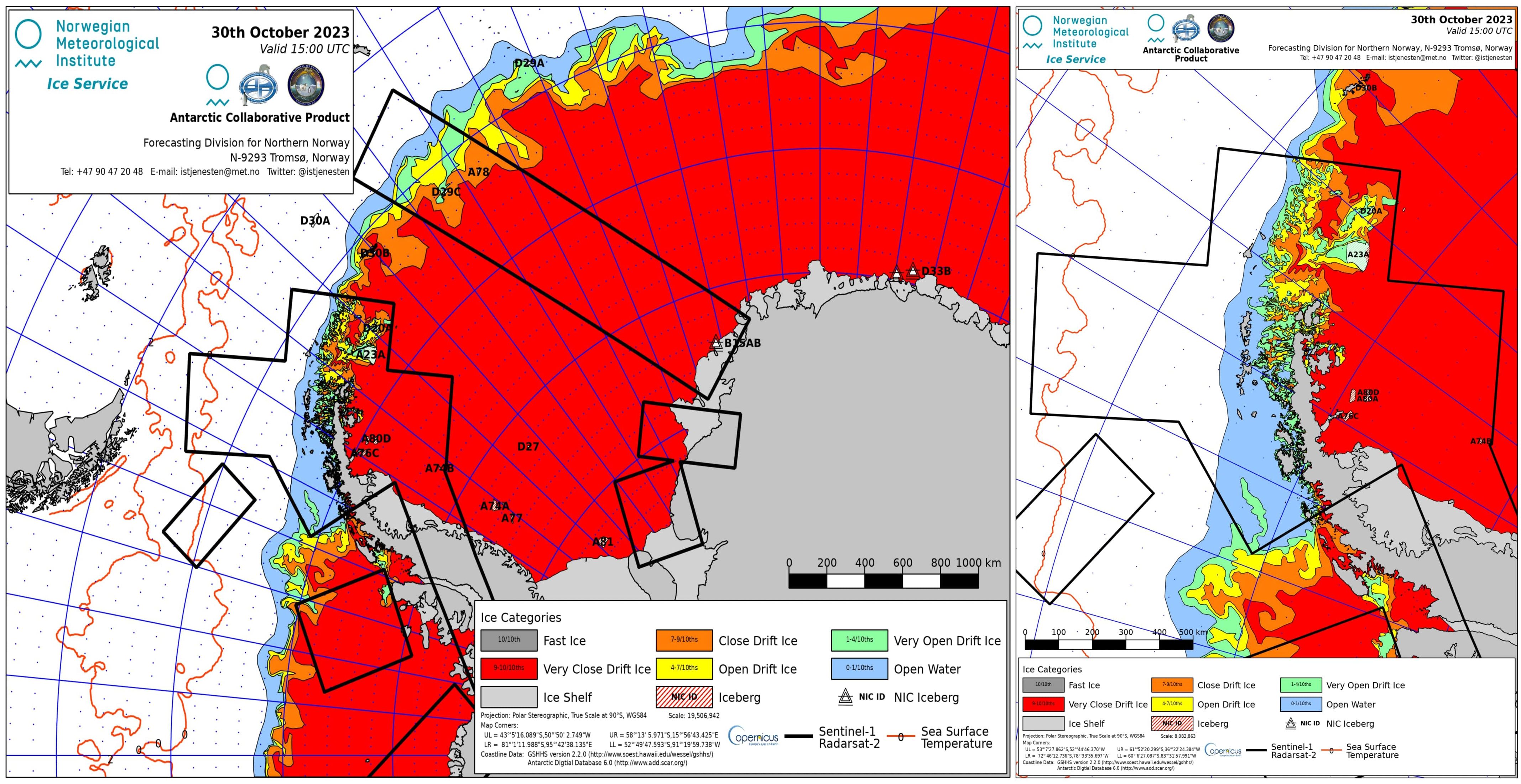
Figure 3. Antarctic ice chart area primarily focusing on the Weddell Sea and Peninsula region where the highest ship traffic takes place during the austral summer.
In the Antarctic, FYI is the predominant stage of development (SoD). This SoD is susceptible to rapid development and decay, rendering its temporal evolution difficult to ascertain solely from sporadic satellite data (Eayrs et al., 2019). Conversely, old ice, which has persisted over multiple years, is relatively scarce in the Antarctic, primarily confined to limited regions in the Weddell and Ross Sea gyres. However, this is reducing due to the impact of climate change (Turner et al., 2020; Shi et al., 2021; Melsheimer and Spreen, 2022).
Despite the SoD not being of primary concern in the creation of ice charts of SIC, the dominance of FYI, drift and the ice edge creates challenges in accurately monitoring ice in near real time (NRT) (Eayrs et al., 2019). This highlights the high competence needed for sea ice analysts with regards to weather patterns and local knowledge, especially where weather has significant interplay with oceanographic or topographic features. Polynya formations are a well-known feature of Antarctic sea ice throughout the formation and melt seasons (Barber and Massom, 2007; Kern, 2009; Campbell et al., 2019).
An additional hazard is the very high density of icebergs, bergy bits and growlers around Antarctica, extending many 10s of km away from the ice shelves. Monitoring of icebergs is carried out by the U.S. NIC and the Argentine Naval Hydrographic Service, where the latter uses both in situ and satellite observations (Scardilli et al., 2022).
3 User needs for ice information in METAREA XIX
Changes in sea-ice regimes in the polar regions are driven by the changing climate, retreating sea ice in some areas and more importantly shifting weather patterns on regional scales that contributes to a high level of variability. There has been an increase in the number of ships observed in polar waters, and this trend is expected to continue in all areas of the Arctic, based on ship-building statistics from the Russian Maritime Register of Shipping, 2024 and Dawson et al., 2022.
Extensive studies have been conducted on the needs of mariners and land-based users in the European Arctic (Kepler D1.1 (Wagner et al., 2019), 1.2 (Mustonen et al., 2019), 1.4 (Hughes et al., 2020), D4.1 (Kangas et al., 2020), 4.3 (Tietsche et al., 2020); Jeuring and Knol-Kauffman, 2019; Jeuring et al., 2019; Stewart et al., 2019; Stocker et al., 2020; Veland et al., 2021; Blair et al., 2022).The recurring theme among end-users is a growing provision for augmented sea-ice products that significantly enhance current operational sea ice information. This includes parameters such as sea-ice SoD/ice type, areas of deformation, sub-daily ice concentration information, and, most Importantly, short-term sea ice forecasts on the spatial scales relevant to the users (Wagner and Hegelund, 2020; Veland et al., 2021).
3.1 Tailoring ice services to diverse user needs
Ice services directly engage with users and stakeholders, regularly documenting user feedback as part of their service. In the European Arctic, users of ice information vary significantly based on their activities, which can be related to maritime or land-based community requirements, as well as their individual levels of expertise. Land-based users require information about the ice’s location and its stability over water. Maritime users navigate through different ice regimes, which may be within the ice pack, around the outer ice pack area, along the edges of ice-encumbered regions, or with the goal of avoiding ice conditions altogether. User needs are not straightforward because they depend on the specific activity, and often, the information requirements and activities overlap in terms of spatial and temporal scales.
One aspect of the IMO Polar Code (Deggim, 2018) concerns the voyage planning component, where the vessel master must be well-prepared for any environmental conditions along the planned route and ensure that the ship is equipped in accordance with the Polar Code. A basic level of competency for the crew is essential, and it is expected that the vessel receives regular and high-quality updates on weather, ocean, and ice conditions for navigational safety and situational awareness.
The ice information requirements of end-users and stakeholders in the European Arctic are influenced by their proximity to the ice edge or ice-covered areas and their varying levels of skill and vessel capabilities. The International Ice Chart Working Group (IICWG) mariner survey provides a concise overview of how these factors relate to how users perceive ice information Table 1 (Veland et al., 2021).
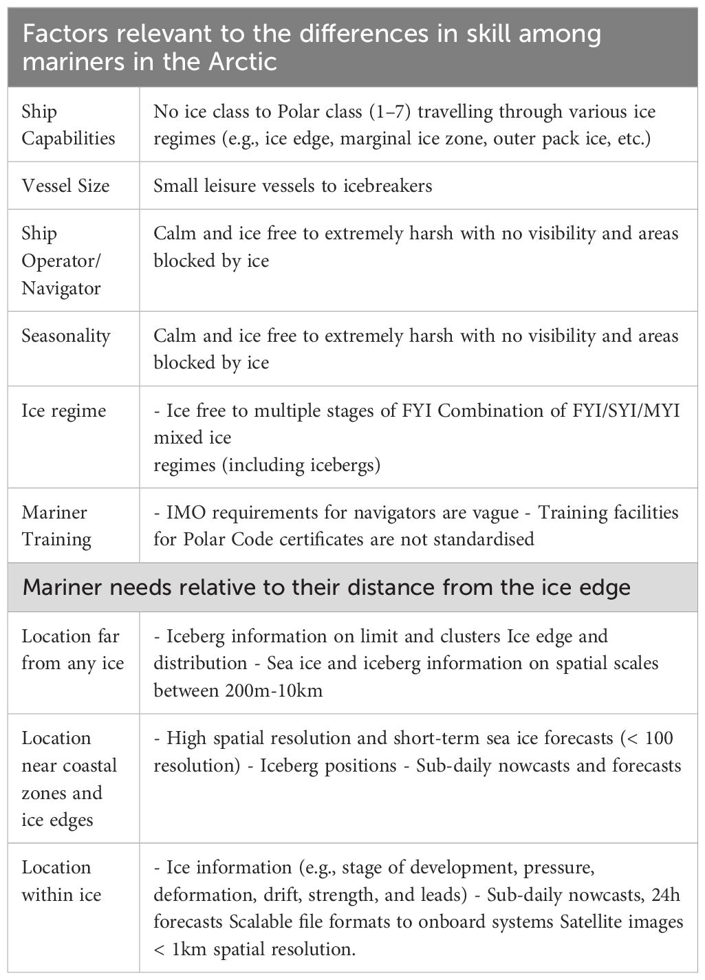
Table 1. Overview of the findings from the IICWG Mariner Survey 2019; Veland et al., 2021 and summer seasons (Sandven et al., 2023).
3.2 User hazards and mitigating ice service requirements
Operating conditions on or around sea ice can turn hazardous at any time due to prevailing weather conditions, and require that ice services ensure information that is sent out is relevant, representative of actual conditions, reliable and accessible. These are part of mitigating measures that underpin the usefulness of the data for end-users. Figure 4 summarises the spatial and temporal scales relevant for the various applications and operations.
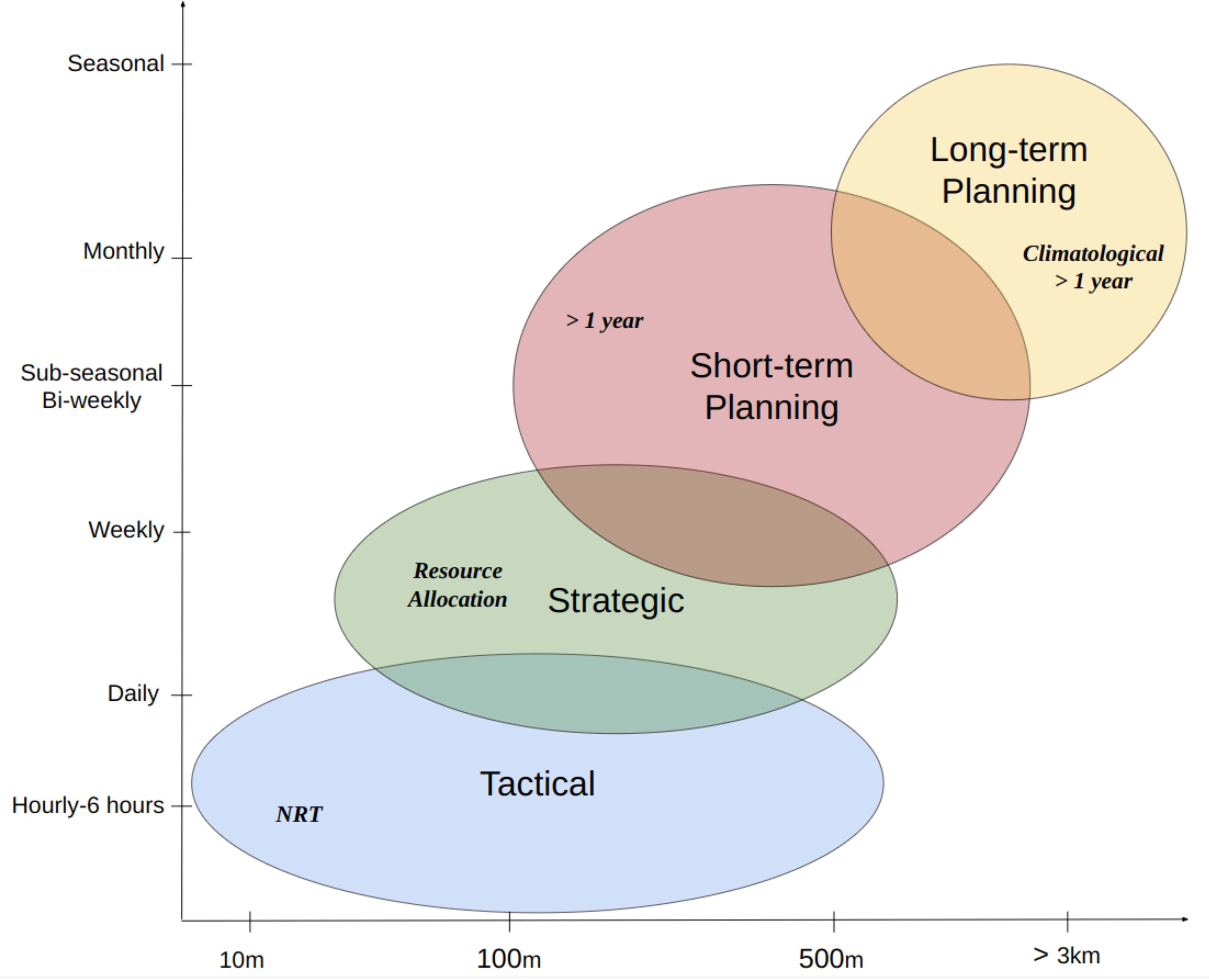
Figure 4. Different situations and corresponding spatial and temporal scales required by the maritime and land use sectors. (Taken from Hughes et al., 2020).
Ships operating in the Arctic Seas continue to experience limited communication bandwidth when at high latitudes (over 75N [with exceptions]) or when ships are travelling in mountainous coastal regions with narrow fjords. This means product dissemination should be clear so the user understands the difference between products, including the quality and relevance to their activity. All ice services aim to provide daily and sub-daily ice information for critical areas (near harbours, choke points); and high resolution products (< 1km) that represent sea ice at the scale necessary to observe features such as ice edges, SoD, deformation and areas of open water. This is particularly challenging given the geophysical caveats observed during the melting of snow on sea ice. As the snow transitions into water on the ice surface, microwave sensors struggle to effectively separate open water, thin and thick ice, impacting the ability to measure sea-ice volume, a key factor in understanding changing sea-ice trends (Tilling et al., 2018; Landy et al., 2021). These limitations are especially pronounced during the melt.
Maritime traffic is increasing with the melting sea ice, especially in the European Arctic, where a mixing of old and new ice regimes continue to be susceptible to ocean and wind forcing. For this reason, a high level of quality control is required to oversee sea ice information that analysts in ice services use prior to being disseminated to the public. Ice analysts closely monitor ice along northeast Greenland where a combination of new melting ice from breakup of the fast ice and old ice flowing out of the Arctic through Fram Strait begin to mix to create larger ice floes. Generally, the thick compact first year ice and old ice north of Svalbard begins to become less compact as the melt season advances towards the summer. This introduces a higher risk for ice advection in the fjords to the north, as well as along the eastern part Nordaustlandet where the ice can be pushed up Hinlopen Strait, depending on local weather conditions.
The vulnerability of sea ice to unexpected displacement during this period creates a misunderstanding between where there are areas of open ice and opportunities for maritime activity in the Arctic. With a lack of observational data in the polar regions, reliability of weather and ice forecasts is reduced (Lawrence et al., 2019; Laroche and Poan, 2021). On the one hand the possibility for more areas of open ice encourages a higher potential for various types of vessels to traverse through regions that are normally ice covered throughout the year. On the other hand, from a user perspective, this creates an operational challenge because in the event of sudden or unpredictable weather conditions, commonly occurring in polar regions, ice can become a hazard if large amounts are quickly moved in the area of a vessel that does not have the appropriate ice class, or if the maritime activity is operating in an area and is unable to obtain appropriate ice information to safely navigate to a safer area.
Therefore there is a critical need for ice services to increase their portfolio to include a variety of relevant products and services that can address a broad group of users with targeted and relevant sea-ice information. The ideal ice service includes the following attributes:
● Ice information that is specific to the METAREA where known areas of high traffic are routinely monitored and where the predominant user/stakeholder community is closely aligned with the ice service products and mandate.
● Sea ice information provided at required resolutions for maritime navigation.
● High update frequency with capabilities to observe hazardous ice (scale: 100–200m or less, sub-daily updates for certain regions).
● Full coverage of satellite data at sub-kilometre resolution for ice charting.
● Tailored/high resolution ice information provision for certain dynamic or critical locations linking to early warning systems.
● Ice information products that can be translated or integrated into risk assessment schemes.
● Local/regional high spatial resolution sea ice forecast products covering 24–48 hours for safe/efficient navigation in/near ice.
● Improved access to scalable ice information and maintain graphical formats for other displays.
● Extended access to automated/annotated satellite Quicklooks.
4 International and national collaboration
The NIS works as a bridge between institution-based projects which aim to develop new products through deep learning/AI methods, and ice service end users. Our role is primarily to provide input from an operational standpoint and help evaluate the algorithms for usability in the operational community. Collaborative efforts are taken both internationally and nationally. Within the NIS the internal development structure provides a crucial role in evaluating product performance. This involves utilising large data volumes and utilising the expertise of the ice analysts, to identify areas for improvement and streamlining the product-to-service chain.
Since the inception of IICWG in 1999, the NIS has been a key member of the Group. The NIS takes part in, and leads, a number of task teams with diverse objectives, including iceberg modelling, implementation of new satellite sensors for operational use, best practises, their usage, gaps and opportunities.
Close collaboration also exists between the International Hydrographic organisation (IHO), International Maritime Organisation (IMO) and the World Meteorological Organisation (WMO). Within the WMO, the NIS plays an active role within the Global Cryosphere Watch (GCW), Sea ice Watch (SIW) which strives to consolidate requirements for sea-ice monitoring, analysis and forecasting, as well as updating WMO guides for instruments and observation best practices. The NIS is also in the Standing Committee on Marine Meteorological and Oceanographic Services (SC-MMO) where the Expert Team on Maritime Safety (ET-MS) maintains the documentation and data standards on sea-ice reporting, including the Sea Ice Nomenclature laid out by the Sea Ice 2014; JCOMM Expert Team on Sea Ice, 2014; International Hydrographic Organization (IHO), 2014).
5 Information sources for ice charting
The creation of ice charts is primarily reliant on the delivery of timely and reliable satellite image data. This is supplemented with in situ, ship-based and aircraft observations, that are sparse in the region due to the logistical challenges posed by the remoteness of data collection in polar regions. All of these data sources are assessed by experienced ice analysts and the information collated into the ice charts.
5.1 Information sources
Over time, the availability of satellite data has significantly expanded, resulting in a wide variety of increasingly higher spatial resolution imagery with varying sensor capabilities. Figure 5 illustrates the evolution of satellite missions, while Table 2 provides a more in-depth overview of the capabilities of SAR imagery specifically. The European Sentinel-1A is currently heavily relied upon for its daily imaging capacity due to a malfunction of its twin satellite Sentinel-1B in December 2021. Improved coverage will be restored when Sentinel-1C is successfully launched (scheduled for November 2024) and after a 6 month commissioning phase.
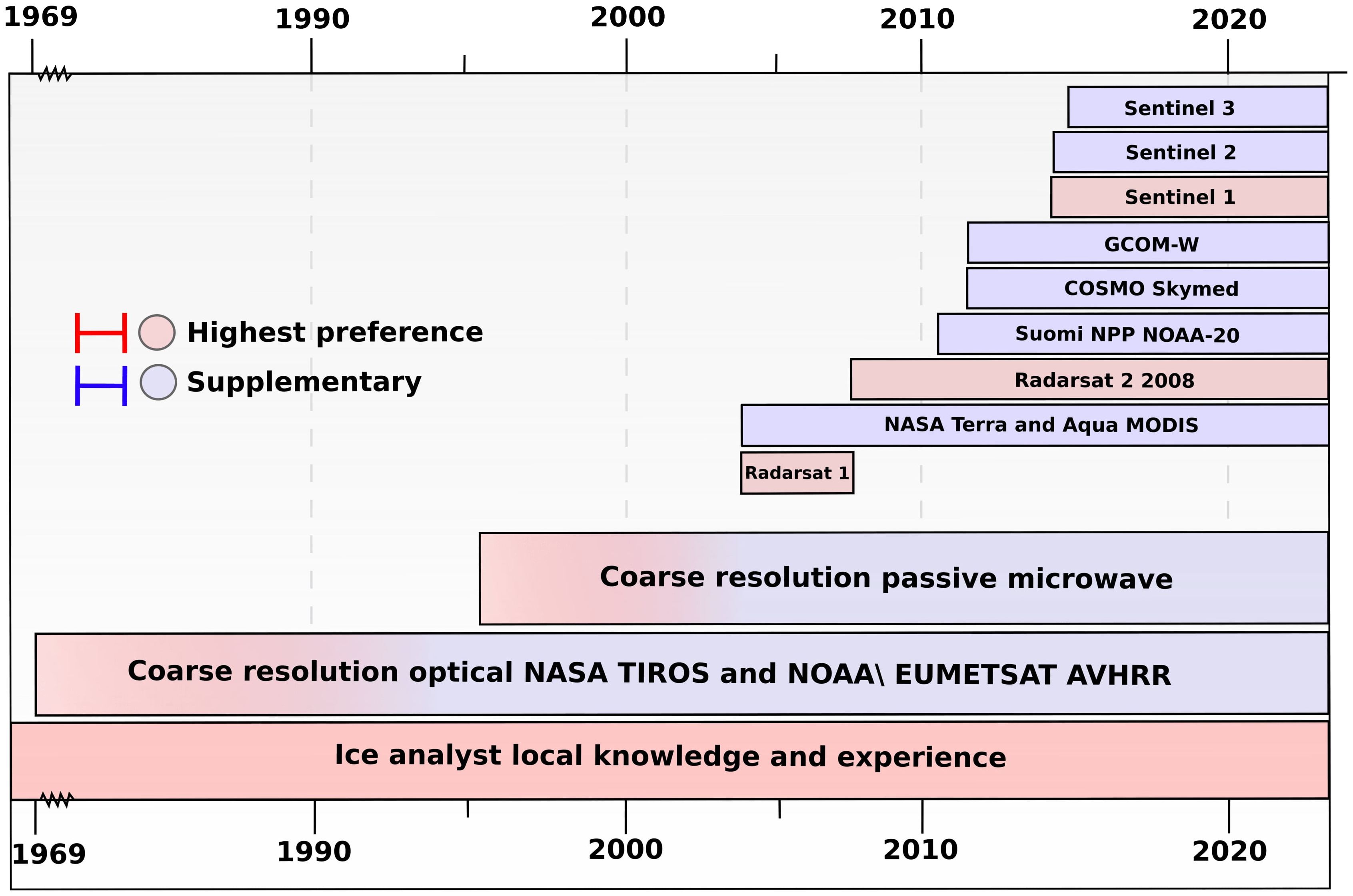
Figure 5. List of satellite data sources as of summer 2022, ranked in order of preference (highest first). Note that ice analyst local knowledge and experience is ranked as highest preference throughout the time period and will continue to be so into the near future even with the initiation of AI and machine learning techniques.
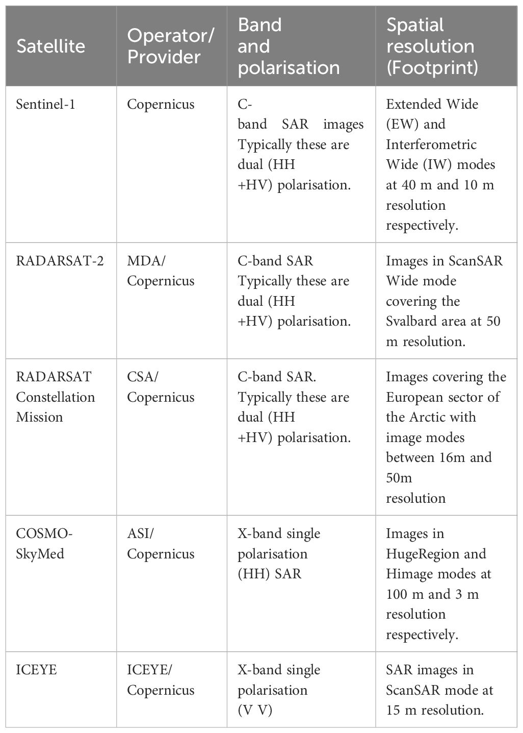
Table 2. SAR sources.
Presently, any gaps in orbital coverage in Sentinel-1A imagery are filled using supplementary SAR imagery from RADARSAT-2, RADARSAT Constellation Mission (RCM), COSMO-SkyMed, as well as optical images from VIIRS, Sentinel-2, Sentinel-3, and METEOSAT Advanced Very High Resolution Radiometer (AVHRR), provided that weather and lighting conditions allow. Passive microwave imagery from AMSR2 is also employed as a guide and supplement to the above-mentioned sources.
5.1.1 Synthetic Aperture Radar
Since the 1980s, Synthetic Aperture Radar (SAR) has emerged as the preferred sensor type for global ice services, first as airborne systems and later on satellites (Haykin et al., 1994). SAR is favoured for its independence from the restrictions imposed by cloud cover and daylight, which hinder the use of optical imagery (Sandven et al., 2023). With resolutions ranging from 3 to 100 meters and wide swath widths of 20 to 400 kilometres, SAR allows for detailed analysis of large areas, depending on the satellite acquisition mode. This capability enables ice analysts to cover extensive regions without the need for secondary sources (Dierking, 2013).
SAR systems can utilize polarimetry to provide information on the orientation of the electromagnetic field vectors, allowing for enhanced analysis of the geophysical properties of the observed surface (Shuchman et al., 2004; Dierking, 2013). A multi-frequency and multi-sensor approach has demonstrated the capability to derive automated sea ice concentration and SoD products that support operational ice services (Singha et al., 2018; Khachatrian et al., 2021; Salvó et al., 2023). This approach can potentially resolve regional and seasonal challenges that have notably hindered the accuracy of sea ice monitoring, particularly during the spring and summer seasons, due to the melting snow atop sea ice and melt ponds (Casey et al., 2016).
The penetration depth of the SAR C, L, and X-band frequencies varies, enabling more accurate 3-D mapping of the ice. Optical and infrared visible sensors complement this data to provide a more realistic observation of sea ice SoD (Lohse et al., 2020) and concentration (Singha et al., 2018; Zhang and Hughes, 2023).
At the NIS, C-band Sentinel-1 and RADARSAT-2 are the primary sources of microwave imagery for ice chart production.
L-band SAR is expected to offer significant improvements for SoD classification, and we have evaluated data from ALOS-2 (Singha et al., 2018; Færch et al., 2023) and SAOCOM satellites in preparation for expanded coverage expected from the future NISAR and ROSE-L missions, set to launch in early 2024 and 2028, respectively.
5.1.2 Optical satellite imagery (infrared and visible)
When available, optical imagery is the preferred supplement to SAR images for ice analysts because features and boundaries are more defined and are easier to identify compared to other forms of imagery. However, its use is limited by the constraints of the polar night and periodic cloud cover.
The main sources for optical imagery are listed in Table 3. The NIS utilizes optical satellite data sources from the Visible Infrared Imaging Radiometer Suite (VIIRS) on the NASA/NOAA Suomi National Polar-orbiting Partnership (Suomi NPP) and NOAA-20 satellites, the Ocean and Land Color Instrument (OLCI), and Sea and Land Surface Temperature Radiometer (SLSTR) on Copernicus Sentinel-3, and AVHRR due to their abundance and frequent overpasses. Previously, the Moderate Resolution Imaging Spectroradiometer (MODIS) on the NASA Terra and Aqua satellites was also used. The Copernicus Sentinel-2 satellite carries the Multi-Spectral Imager (MSI) with 13 spectral bands and has a 10-meter resolution within the visible spectrum and a 60-meter resolution in the near-infrared bands. This provides analysts with a very high-resolution overview of the ice conditions in specific locations, complementing the resolution available from SAR. This high resolution is especially important within the complex fjord systems of the Svalbard and North East Greenland regions, where small-scale features such as icebergs can also be identified.
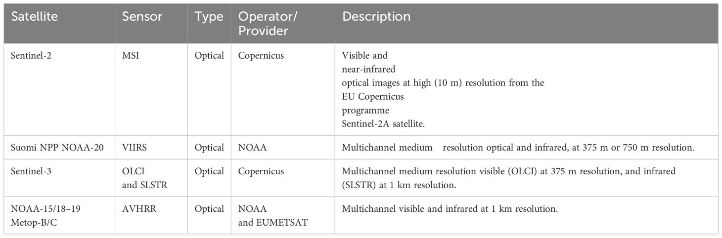
Table 3. Optical imagery sources.
5.1.3 Passive microwave
Passive microwave sensors (Table 4) provide valuable data products that are utilised primarily in climate analysis, particularly for observing sea-ice concentration and extent over long time scales, and more recently, thin sea ice thickness through L-band radiometry (Heygster et al., 2009). Despite being available year-round, this data is typically only used as an aid to ice charting during the Northern Hemisphere winter for latitudes north of 60°N, when optical images are no longer viable due to limited daylight hours, or in the Southern Hemisphere, where SAR coverage is sparse. The Advanced Microwave Scanning Radiometer (AMSR-2) sensor, onboard the GCOM-W satellite, is the primary used in these instances (Meier and Stroeve, 2022). When the data from AMSR-2’s 89 GHz channels are processed to 3.125km (e.g. Spreen et al., 2008), the data can be of use with quality control from an analyst and in the absence of SAR and optical imagery.
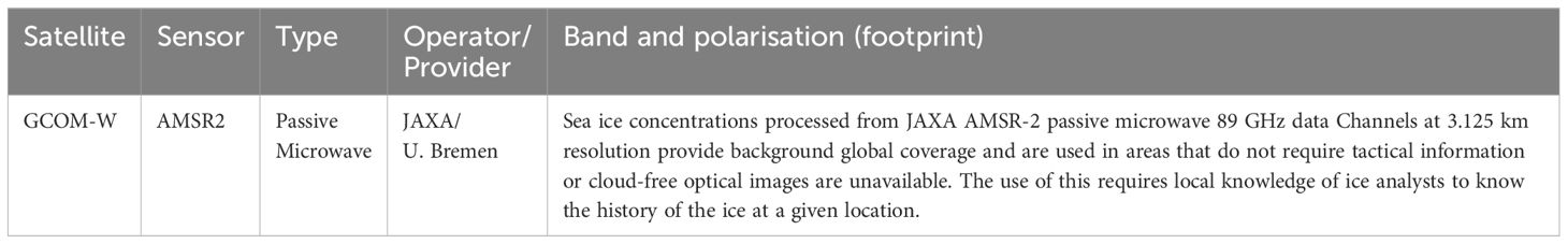
Table 4. Passive microwave imagery source.
6 Sea ice analyst knowledge on local and regional scales
Ice analysts not only interpret satellite imagery but also apply their inherent understanding of weather conditions and utilise past experience, and local knowledge when creating an ice chart. This section aims to emphasise the importance of having ice analysts in all ice service teams to ensure the most reliable ice chart is delivered to our end users, even with the advent of artificial intelligence (AI) and machine learning techniques.
6.1 Sea-ice development, dynamics and decay
Interpreting sea-ice conditions from satellites requires skill that involves integrating insights from local environmental systems to understand ice formation and decay. This entails having a proficient understanding of how sea ice develops, encompassing seasonal and regional variations. We provide a short summary here, but the interested reader is referred to the International Hydrographic Organization (IHO), 2014 webpage and Wadhams, 2000.
A typical sea-ice SoD cycle in the northern hemisphere starts in mid to late September, with freeze-up, and continues through to the next summer. Freeze-up begins when the surface sea water is cooled to around -1.8 °C, for water with average salinity of 35 psu (practical salinity units). The first indication of sea ice formation begins with small ice crystals, frazil ice, forming in the water. Under calm conditions, these coalesce into grease ice, and in the presence of waves, into pancake ice. Both of these types of sea ice are distinctly recognisable, both visually, and in SAR images. Further cooling under calm conditions results in increased ice thickness, and a thin sheet called Nilas ice is developed. This can be subdivided into dark (thin, up to 5 cm) and light (thicker, up to 10 cm) nilas. Waves result in increasingly thick, and large floes of, pancake ice. Both nilas and pancake ice may thicken further and floes freeze together to form grey (up to 15 cm) and grey-white (up to 30 cm) ice. So far the ice crystals in all these types of sea ice, collectively known as Young Ice, are still randomly orientated due to their frazil origin.
The next stage of development is FYI, and thickening occurs through columnar ice crystal growth on the underside of ice floes. Thin FYI is 30–70 cm thick, medium FYI is 70–120 cm, and thick FYI is up to 200 cm, a limit imposed by onset of melting in the spring. All of these types of FYI are also distinct in high resolution satellite images, with thin FYI having smooth surfaces, often confused with calm water in SAR images, medium FYI having small ridges, and thick FYI having large ridges. In areas of high snow accumulation, typically in the Antarctic but also in some locations in the Arctic, the snow load can push the ice surface below sea level, resulting in flooding and the growth of superimposed ice.
When air temperatures go above 0°C in late spring or early summer, the melt season begins. Snow that has accumulated on the ice surface melts and forms puddles, called melt ponds. These are darker than the surrounding ice and absorb solar radiation, causing enlargement of the melt pond and eventually penetrating through to form thaw holes. For this reason, analysts consider that the melt and freeze-up periods are expected to vary regionally, when assessing the current ice situation.
FYI can survive a summer melt season and is then classified as Old Ice. This can be divided into SYI and MYI. The melt season causes the ice to become less saline due to brine drainage, and air pockets in the ice being removed. This increases the hardness of the ice, and MYI embedded within FYI is therefore a significant hazard to marine users. MYI is also distinct from FYI in both optical and SAR satellite images.
An example of some varying ice regimes and types can be seen in Figure 6 from the CIRFA cruise in Spring 2022. These were observed both by Sentinel-2 optical and Sentinel-1 SAR and compared to in-situ imagery taken as part of the Ice Watch program Ice Watch ASSIST Data Network, 2006.
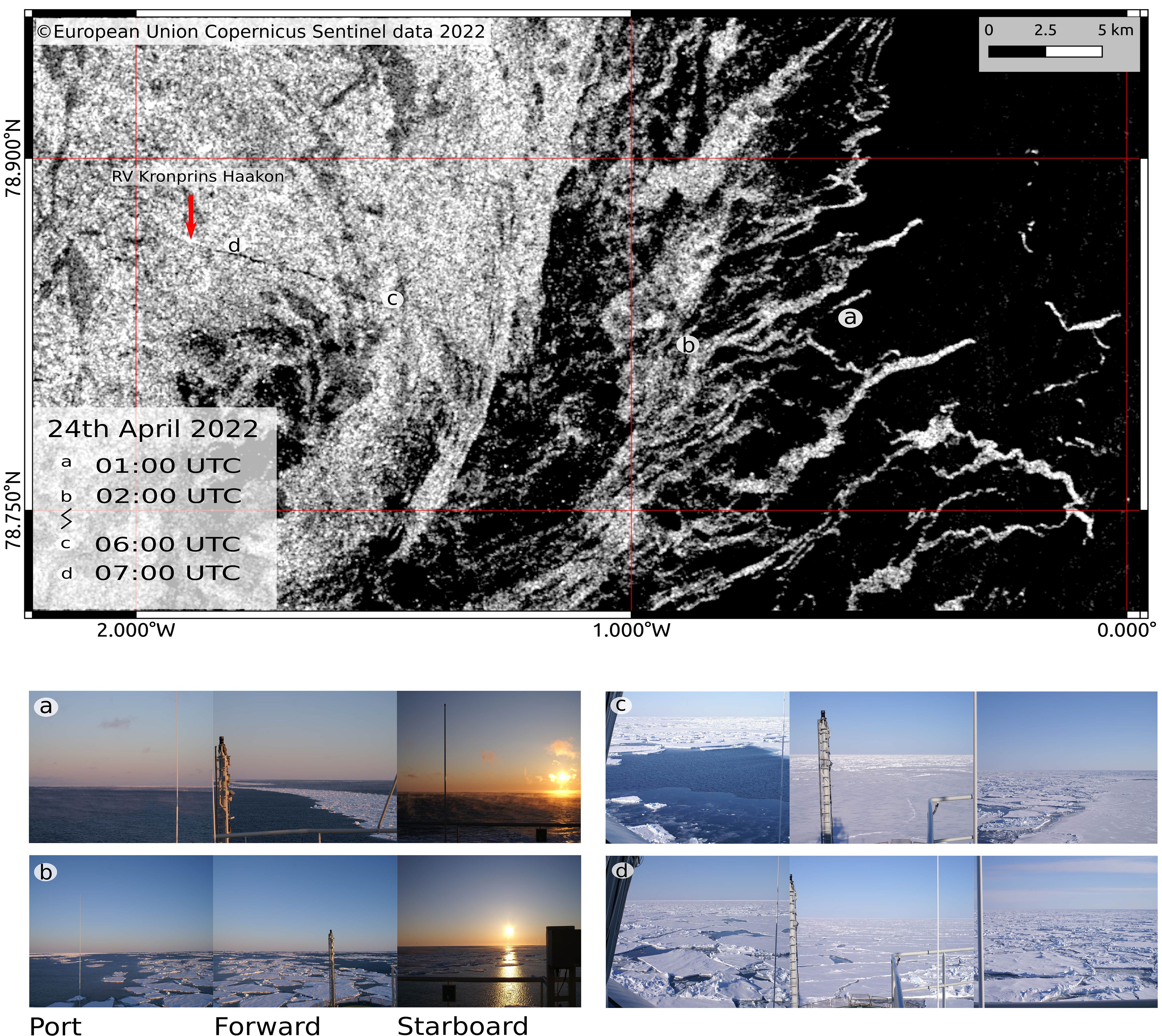
Figure 6. SAR imagery for 24th April 2022. Ice Watch imagery location aligned with satellite imagery to show in situ conditions (Ice Watch ASSIST Data Network, Norwegian Meteorological Institute, 2023). The markers a-d show the locations at which photographs were taken, which can be seen under the satellite image. (Copernicus sentinel data 2022, processed by ESA).
6.2 Inter-annual variability
Within METAREA XIX, interannual variability is becoming increasingly prevalent in response to climate change (Serreze and Stroeve, 2015; Onarheim et al., 2018; Lundesgaard et al., 2021; Luo et al., 2023; Sumata et al., 2023). Figure 7 shows the variability of ice conditions from the ice charts over the period 2012–2023 for the end of various months through the year around Svalbard. It is evident that interannual variability can be significant, creating challenges in providing reliable long term forecasting of ice edge positions on an annual to interdecadal time scales. Most of these large variations are due to shifts in weather patterns which need to be understood by ice analysts in order to update the ice chart accordingly.
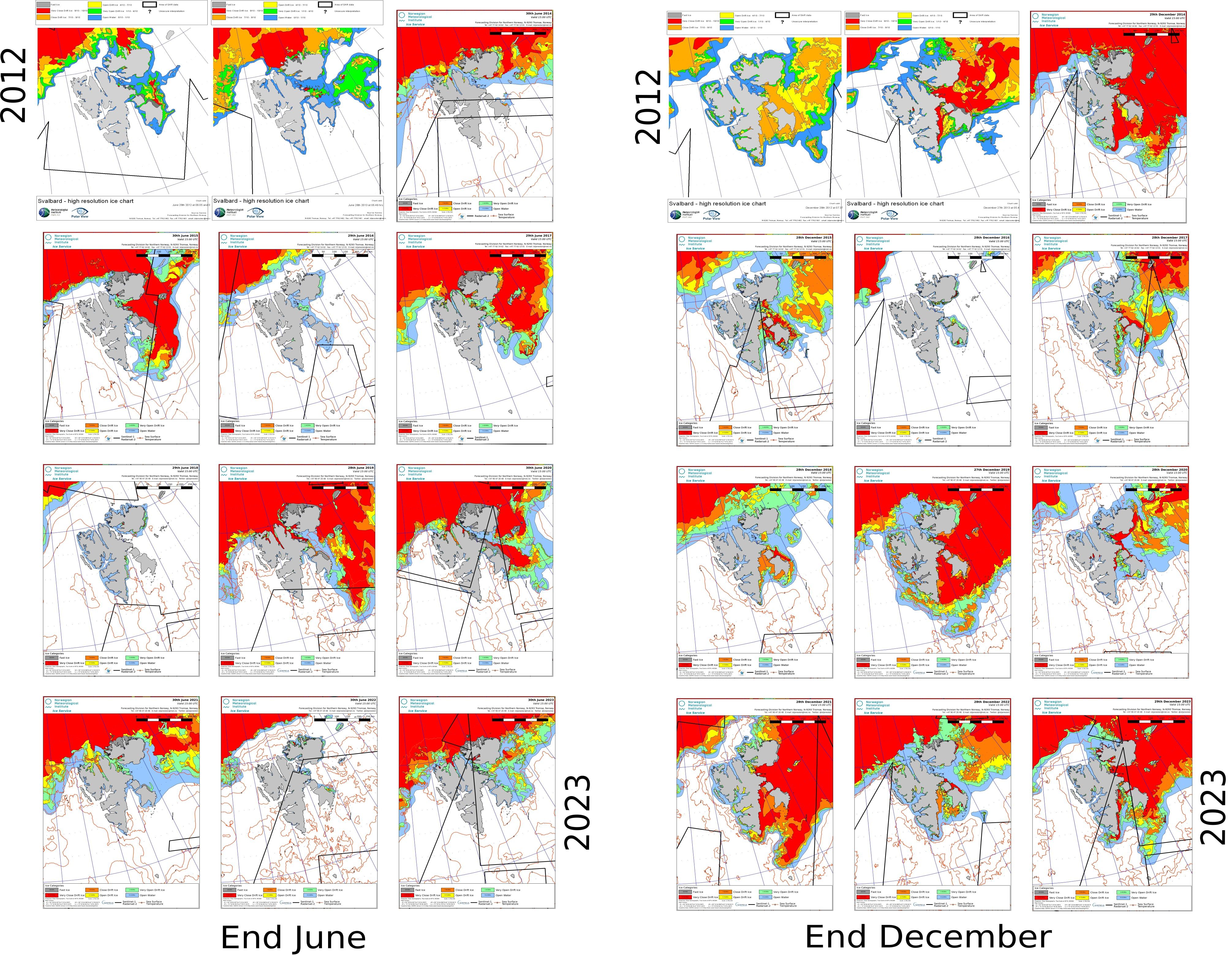
Figure 7. Variability of ice conditions from the ice charts for summer conditions (late June - 28-30th) and winter conditions (late December - 27-29th) over the period 2012–2023 around Svalbard. There is quite clearly a large range of inter-annual variability over the last decade, which can be explained by prevailing winds over the course of weeks or months resulting in drift and formation of ice around the archipelago.
6.3 Regional sea ice changes due to weather impacts
Over short time scales (1–7 days) the effect of large fluctuations in temperature and wind and wave action can have a significant impact on the ice edge and how sea ice and surrounding ice free water appears in satellite imagery. This is where the skill of the ice analyst is vital, as they are able to distinguish between ice and water, and identify surface characteristic changes of the ice. AI and machine learning techniques struggle to find consistent patterns that accurately represent the current ice situation, emphasizing the importance of tracking ice history through ice analysts as displayed in the Extreme Earth Project, 2021. During intense weather events, the risk of ice advection in unexpected areas rises. Therefore, timely and reliable ice information is crucial.
METAREA XIX experiences significant weather fluctuations due to its exposure to Atlantic low pressure systems. In addition, very cold air masses moving over the warmer waters that flow northward into the West Spitsbergen Current create the perfect environment for polar lows, a defining polar weather system that can rapidly affect the sea ice edge state of an area within the space of just a few hours (Rojo et al., 2015; Mallet et al., 2017).
Figure 8 shows the effects of strong katabatic winds flowing south eastward from north east Greenland creating a polynya along the fast ice (FI) edge in early May 2022. Sea surface temperatures and air temperatures were conducive to sea ice formation. There is a clear indication of pancake ice formation due to the combination of strong wind and ocean forcings. As a result, the corresponding SAR image demonstrates challenges to decipher the presence of sea ice in a given area, due to rough surface conditions/reflectance. By the 4th May, winds had calmed slightly allowing pancake ice to cement, significantly reducing wave action and therefore resulting in a more flat reflectance signal in the SAR imagery. As can be seen in the optical imagery (left), both days have similar sea-ice concentrations within the polynya, however, this is difficult to perceive from SAR imagery alone. Without analyst knowledge of the area, weather conditions and continuity in monitoring, misinterpretation of these two images without the help of optical imagery (such as in the winter or with cloudy skies) would be very likely.
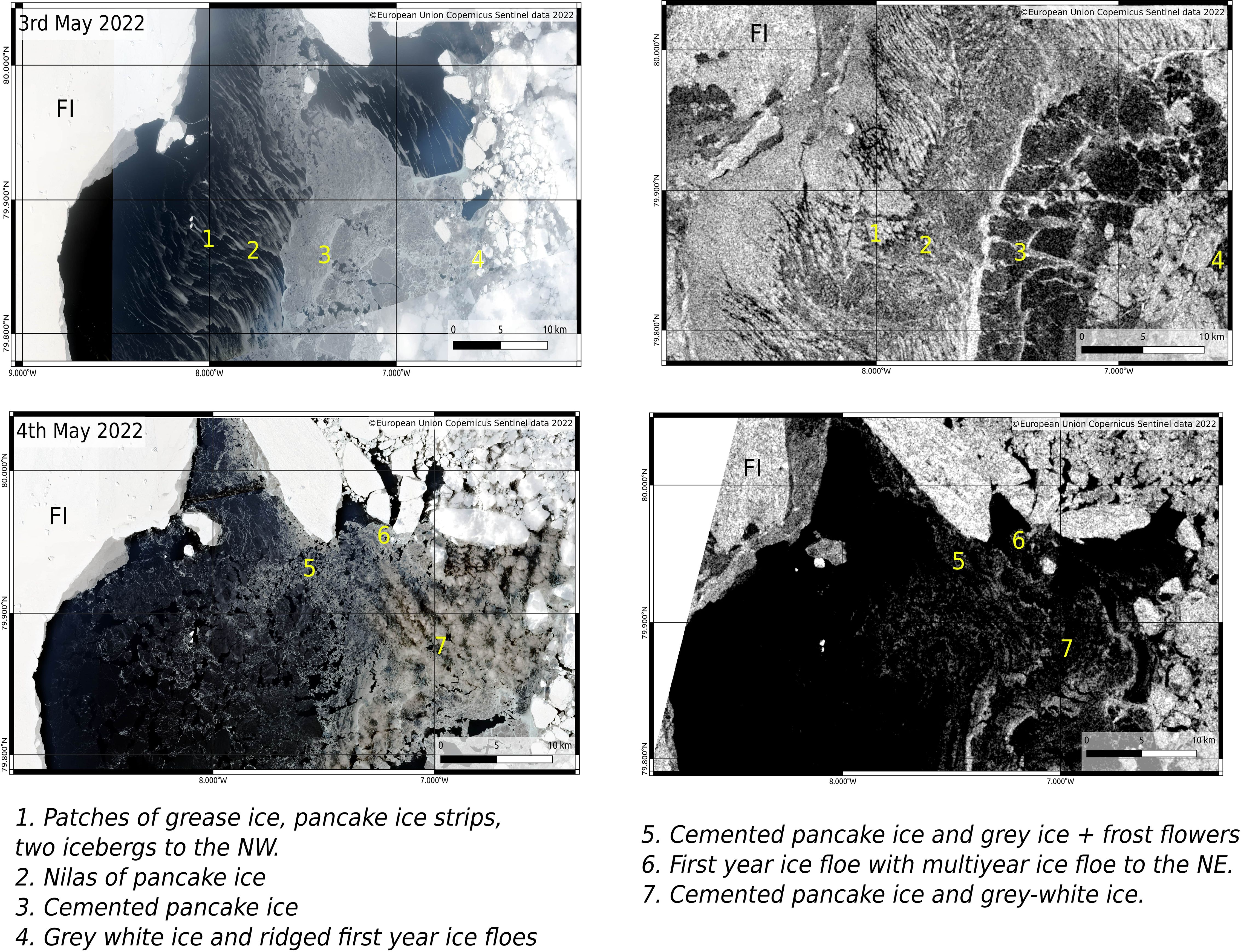
Figure 8. Ice watch observations versus satellite imagery for 2 consecutive days. Sea ice SoD and concentration (expressed in 10ths) stated for specific locations along the track of RV Kronprins Haakon in Spring 2022. (Copernicus sentinel data 2022, processed by ESA) (CIRFA research cruise 2022).
7 Construction of sea ice charts
The NIS produces routine ice charts for the Arctic from Monday through Friday, as part of its operational mandate for METAREA XIX. The ice charts nomenclature and colour code standards follow the WMO, 2004 Ice Chart Colour Code Standard (WMO/TD-No. 1215) and Sea Ice, 2014 Sea Ice Nomenclature (WMO-259) documents used at all ice services. Ice chart production at the NIS relies on manual analysis from expert ice analysts due to the geophysical limitations of sea ice monitoring as outlined in section 5. Currently, the sea ice charts represent sea ice concentration, ice edge and delineation of fast ice areas.
7.1 Tools and systems
Geographical Information Systems (GIS) software serves as the standard ice charting system for all ice services. It allows for scalable data representation and standardized vector data formats that seamlessly convert to S-411 (ice information product specifications laid out by the IHO) and sea ice grid (SIGRID) standards. This compatibility is vital for users needing information to be transmitted through electronic navigational charts (ENC) onboard ships or in the field. The analysts are supported by a selection of systems designed to automate a number of tasks and aid in the production of an ice chart. At NIS these are set up as part of the Bifrost system and run on various parts of the infrastructure at MET Norway.
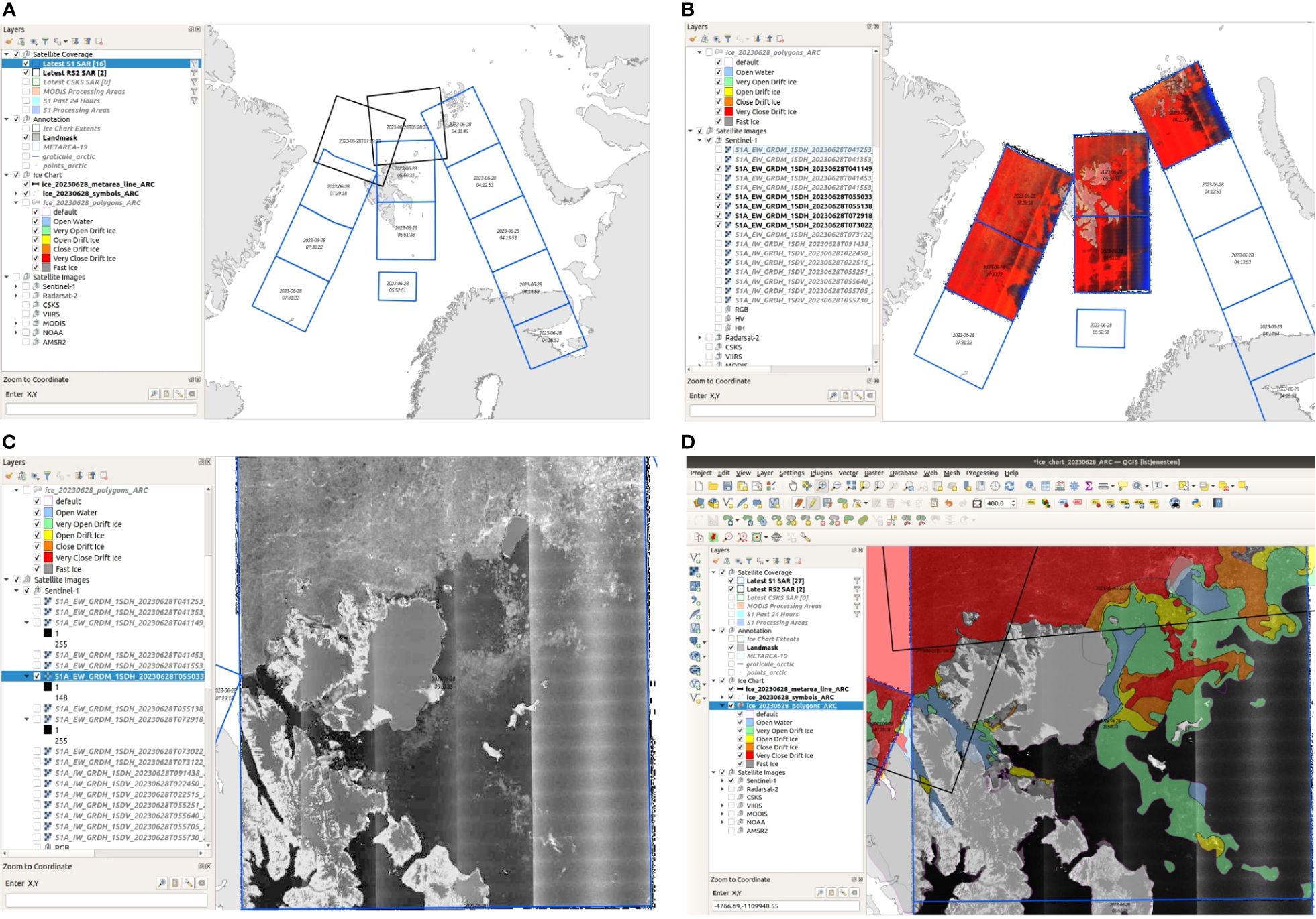
Figure 9. Screen shots showing various stages of the ice chart creation process. (A) Shows the satellite imagery timestamps loaded automatically on opening of the QGIS project. (B) Pre-rendered sentinel 1 SAR imagery selected for the area of interest. (C) Zoomed in and rendered Sentinel 1 SAR image from NE Svalbard. Image rendered by changing render type from multiband colour to single band grey and choosing Band 2 (green band), along with increasing the brightness and contrast under colour rendering. (D) An underway ice chart for the satellite image in c where the analyst is using their knowledge and experience to identify areas of differing ice concentration.
The NIS developed an ice charting system using QGIS, an open source geographic information system (QGIS Development Team, 2023). QGIS includes tools for drawing and editing polygons and overlaying various satellite products. It is also compatible with digital drawing tablets, which some analysts prefer over using the mouse. NIS employs customised QGIS profiles which are installed on the analyst work stations. Each day a project is automatically generated with all the required layers available such that an analyst can quickly begin drawing polygons. On Mondays, a fresh ice chart is generated using only the fast ice extent and the ice edge from the previous Friday, while on subsequent days of the week the chart is a copy from the previous day which is then updated to match current conditions.
The various satellite products outlined in Section 4 are downloaded and processed on MET Norway’s high performance computing cluster. These are then made available on the analyst’s workstation where they can open and view images in QGIS (Figure 9). This processing is almost entirely automated, with the exception of some more bespoke satellite products. Other data used by the analysts, such as weather models and observations are viewed using Diana, a meteorological visualisation and production software developed at MET Norway.
While the ice chart is being drawn, the analyst can run scripts which validate the ice polygons and check for errors which may not be obvious to the naked eye. After the ice chart is completed, the analyst must go through a quality control (QC) process to check the chart, and after this the ice chart can be sent for further processing. This primarily involves the production of the various products outlined in the following section, as well as distribution via email and uploads to various other distribution channels.
Inter comparison between analysts and comparison studies of ice charts against models have been carried out with regards to the inherent subjectivity of ice chart creation, showing positive results (Moen et al., 2013; Karvonen et al., 2015; Cheng et al., 2020).
7.2 The sea ice analyst’s workflow
Producing an ice chart begins with reviewing weather, wind patterns and temperatures from the previous day. The fast ice, attached to land, is updated as needed throughout the week, unlike drift ice, which requires more frequent updates. Ice analysts align with the Canadian Ice Service, 2005 Manual of Standard Procedures for Observing and Reporting Ice Conditions (MANICE).
Using the satellite imagery, the analyst constructs the ice chart by subdividing a large initial polygon into smaller polygons denoted by primary, secondary and tertiary. Each smaller polygon is then assigned its respective ice concentration in tenths.
Additionally, high-resolution satellite images from the previous night are downloaded, particularly those covering eastern Greenland, to mitigate gaps in satellite coverage later in the day. Analysts receive individual SAR swaths beginning over Nova Zemlya and proceeds westward, ending at NE Greenland. Satellite imagery delivery of individual swaths follow the satellite acquisition from the orbit and the latency is typically less than 3 hours from acquisition to delivery to BiFrost. In exceptional cases, the acquisition is less than one hour for priority swaths from the Collaborative Ground Segment in Norway, or orders through Kongsberg Satellite Services (KSAT).
When drawing the ice chart, analysts prioritize high-traffic areas, focusing on detailed analysis. This includes considering the capabilities of vessels with low or no ice class that travel around Svalbard and snowmobile excursions around Spitsbergen. The sea-ice concentration within individual polygons is determined by tenths of the total ice concentration of an ice area, adhering to the criteria outlined in MANICE and the WMO Egg Code.
Analysts use all available satellite data to assess the current ice situation. Upon completion of analysis on all imagery, the polygons are quality checked for any invalid polygons or nodes. In areas with gaps in SAR coverage, lower spatial resolution satellite data may be used to supplement. However, analysts possess inherent knowledge of ice precision and can adjust for ambiguities, especially at the Marginal Ice Zone (MIZ) and ice edge. When the ice chart analysis is completed, the Metarea XIX line from southwest Greenland to the eastern part of Franz Joseph Land is drawn. After a quality check for any data errors, the ice chart distributed online. The METAREA XIX line is sent separately into the meteorological weather system. The ice edge coordinates are sent to the coastal radio centre for distribution to fishing vessels. It is important to note that the operational definition of the “ice edge” is considered the line separating open sea from any type of sea ice at a specific time as outlined by the WMO, 2004.
Alternatively, the typical threshold used in climate monitoring is 15 percent, or more, within a 12 - 25km pixel or grid cell. If a pixel or grid cell exceeds 15 percent ice concentration, it is considered ice covered; otherwise it is deemed as ice free. It is important to clarify this distinction when communicating with end-users and stakeholders.
7.3 NIS products
A general ice chart is generated for the entire region, while regional charts for the Baltic, Barents sea, Denmark Strait, Fram Strait, Oslofjord and Svalbard (Figure 10) are also generated from the analyst’s daily chart.
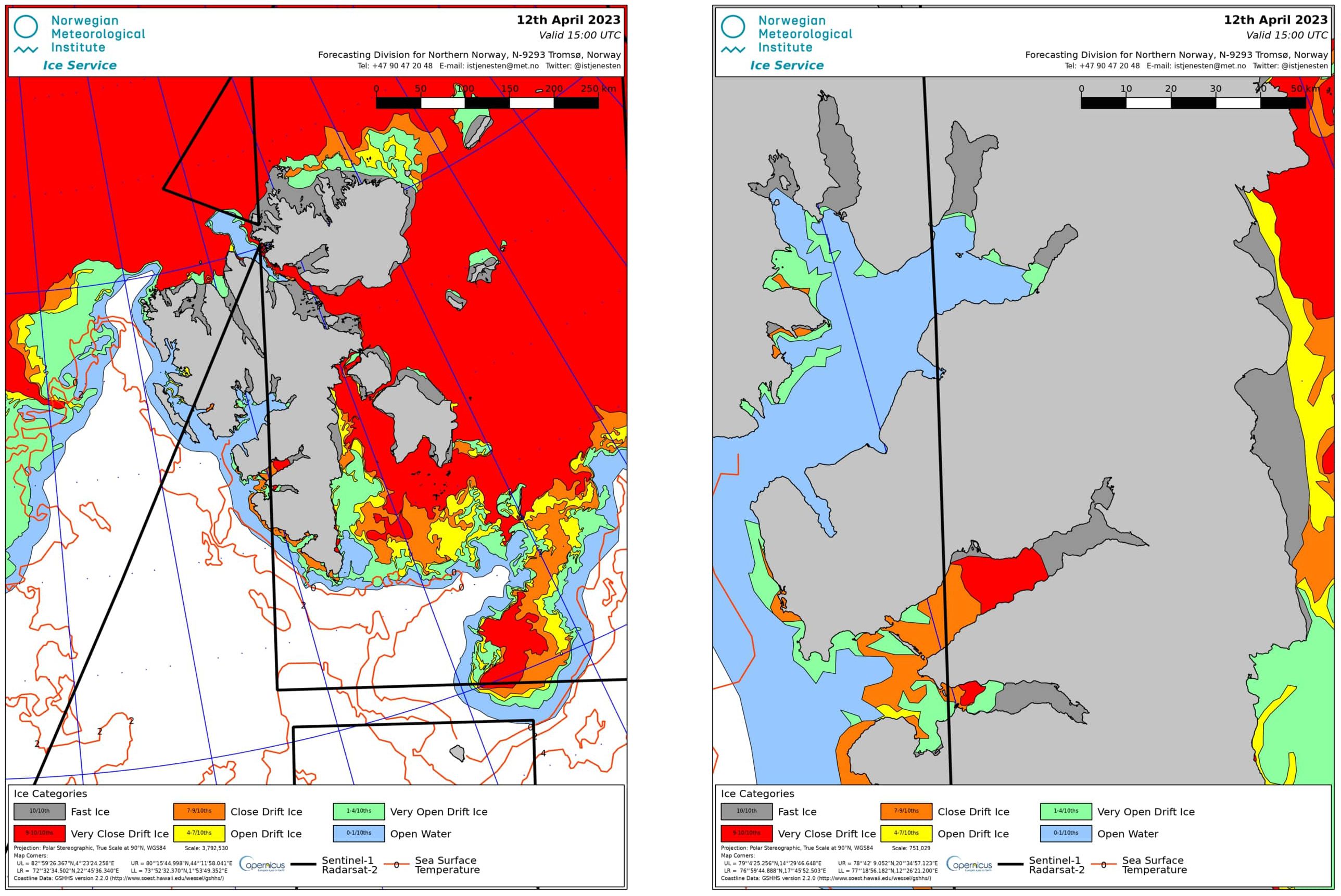
Figure 10. Example of a completed regional specific ice chart for Svalbard. Black bounding boxes highlight where satellite imagery was available during construction of the chart to allow for users to know where the greatest reliability of sea ice information is present. Red contour lines delineating sea surface temperatures are taken from a combination of thermal imagery sources according to the data from E.U. Copernicus Marine Service Information (CMEMS), 2023.
The SIGRID-3 file format is currently the standard for all ice services due to its two main advantages of being compact and scalable. This means vector data typically requires less disk space and can be displayed at varying scales without loss of quality. For ice information relevant for users, this allows for information to be easily retained and catalogued for easy access for maritime users, particularly in the field, which has resulted in the development of the IHO S-411 format for use in Electronic Navigational Chart (ENC) systems.
Users can receive ice charts via email covering any of the available regions in PNG, JPG or PDF format, depending on their available bandwidth. Zipped SIGRID-3 and S-411 files can also be provided to users, but require some GIS or ENC knowledge to use. The ice edge position for METAREA-XIX is communicated via telex. All archived ice charts from 1997-present are stored and available on the website for the ice service, available in JPG format, and as Shapefile upon request. Earlier ice charts from 1967 to 2002 can also be found in ACSYS, 2003. Further products provided by the NIS as of 2023 are listed below and can be found at the MET Norway Ice Service webpage.
● Applications of Research to Operations at Mesoscale (AROME) weather prediction and the Regional Ocean Modeling System (ROMS) ocean prediction models integrate NIS gridded data into their systems, and these are distributed publicly through the MET Norway Thredds server. The gridded products are also disseminated via the EU Copernicus Marine Environment Monitoring Service (CMEMS).
● High resolution charts are available for the Svalbard (Isfjord) area.
● A weekly (Monday) Antarctic chart has been produced during austral summers (October to April) since the 2010/2011 season. In addition, a high-resolution chart is issued for the Bransfield Strait and Adelaide Island areas of the Antarctic Peninsula. These charts are produced in collaboration with the U.S. National Ice Center and Russian Arctic and Antarctic Research Institute.
● Visualisations of external short range, 10 day or less, sea ice forecasts at intervals of 24, 48, 72, 96, 120, 144 and 168 hours. The Global Ocean Forecast System version 3.1 (GOFS3.1), Nansen Center Sea Ice Model (neXtSIM) and Barents-25km models are used due to their spatial resolutions being better than 5km, therefore approaching a scale that can better represent finer sea ice edge detail and conditions within the Svalbard fjords. These products are considered as experimental at this stage due to their external creation, meaning the NIS cannot guarantee availability or accessibility of this product.
8 Discussion - future of the NIS
8.1 Ice charting automation
A number of projects have focused on the automation of ice charting procedures with varying degrees of success so far (Dierking, 2020). However, as of yet there is still no algorithm or products that are used for year round sea ice charting and operationally in ice services. The scope of research and literature addressing this work is vast and out of the scope of the paper but relevant information can be found at (KEPLER Project, 2020; Extreme Earth Project, 2021). The more advanced products are in the beta-testing phase and will require further understanding of how they address specific inter-annual and regional variability within each METAREA as highlighted in the Extreme Earth Project, 2021. The challenges are due to a combination of the complexity of satellite images through the shifting seasons (especially spring and summer) and the patchwork nature of SAR imagery in a given region. Another factor limiting automation of ice charting is the time in which analysts have to create an ice chart. Time constraints leave little time for analysts to evaluate an algorithm output and provide quality control for all the inaccuracies, whereby more time is spent on correcting errors than using the traditional manual method. Continued work with improved coverage of relevant satellite sensors, advanced intelligent AI and machine learning algorithms for sea ice mapping and forecasting, and assessments of the seasonal robustness and applicability to seasonal variability, will lead to more semi-automated ice services and enhanced capacity to service users (Karmakar et al., 2023; Khachatrian et al., 2023; Lima et al., 2023). Iceberg detection is also showing promising results with the Constant False Alarm Rate (CFAR) algorithm for object detection. In combination with known Automatic Identification Data (AIS) which can provide input when carrying out high resolution iceberg forecasting. Meanwhile drift models are providing information about areas of all known ice that can be useful in risk assessment and situational awareness for iceberg forecasting (Kubat et al., 2005; Dagestad et al., 2018; Færch et al., 2023).
8.2 Stage of development charts
Sea ice SoD is currently not routinely included in the ice charts at the NIS, however, ice analysts do take into account the ice age and type during the creation of the concentration charts. This is necessary to provide forecasts to users where they can anticipate drift dynamics in changing weather conditions (e.g. old thick ice is much less likely than thin new ice to drift rapidly with changing wind directions).
8.3 User need for reliable sea ice forecasts
There is an overall need from the operational marine community to have reliable, understandable and easily accessible sea-ice forecasts available at multiple time scales. They assist with strategic and route planning (short-term and sub-seasonal), as well as being valuable for long-term planning or logistics (seasonal). Sea ice forecasts typically assimilate data on the spatial scale of sea-ice climate mapping and models, although more advanced techniques for sea-ice thickness allow for resolutions of 5 or more kilometres. While this is felt by some developers to be inadequate, there are few attempts to push for datasets that are more representative of actual ice conditions due to the time and resources used in setting up and running these models (Blockley et al., 2020; Hunke et al., 2020; Wagner et al., 2020; Andersson et al., 2021; Veland et al., 2021; Müller et al., 2023). Drifting sea ice poses a challenge for sea-ice forecasts to accurately assimilate certain parameters such as sea ice SoD or thickness, and concentration, particularly during the late spring and summer seasons due to snow melt. It is especially difficult to convey sea ice in forecasts at the MIZ and along the coastal areas where due to the merging of satellite products from multiple time points and with varying sensor frequency footprints, there is often a smearing of the ice edge and any features of potential interest. A full review of the current state of sea-ice forecasts is out of the scope of this manuscript but refer to Smith et al., 2019 and Fox-Kemper et al., 2019) for a further overview.
It has been demonstrated that assimilation of ice charts improves prediction accuracy of short term forecasts by providing quality controlled and regularly updated information on ice concentration and potentially stage of development (when available) (Posey et al., 2015; Kvanum et al., 2024). The use of ice charts for initialization into models and forecasts can enable real-time adjustments, that significantly boosts forecasting precision and maritime safety (Hunke et al., 2020).
8.4 Exploitation of new ESA satellite missions
Over the next few years, multiple new satellite missions aim to introduce availability of L-Band SAR. For the NIS, the NASA/Indian Space Research Organisation (ISRO) Synthetic Aperture Radar (NISAR) and Copernicus Radiometer Occultation Scattering Experiment - Lite (ROSE-L) are of most interest. After successful deployment of the satellites, evaluation must take place over the course of the next few years, meaning there is still a delay after the launch date before these satellites are operational. In preparation NIS is engaged in evaluations of the benefits of L-band SAR for sea ice mapping and iceberg detection (Dierking et al., 2022; Færch et al., 2023).
Studies were carried out during the KEPLER project to ascertain the spatial resolution requirements of end users. Results show that the spatial resolution of sea-ice information is of particular concern. The current state of information provision cannot always provide details on sea ice features such as ice type and deformation on the scale that would improve support for the operational marine community; unless it is administered by private or commercial services that need to be prepared in advance. There is a collective need for spatial and temporal resolutions for the Arctic and Baltic operators. New and improved products for the maritime sector are consistently requested in order to provide high resolution ice products based on SAR as well as information on ice thickness and ice type. Table 1 shows the level of interest in spatial scales for different parameters based on whether these were for tactical or planning purposes. High-resolution products for tactical purposes, where high resolution is understood to be on the sub-kilometre scale, are highly sought after. Spatial resolutions on the kilometre scale are of interest at the planning stage for most users, and more commonly in the research community. End-users deemed the kilometre scale too coarse for navigational and tactical use due to the difficulty in detecting features important for maritime operations such as ice concentration at the edge, the marginal ice zone and coastal zones, ice concentration, leads, polynyas and icebergs. In addition, a number of intermediate users noted that this spatial resolution was an impediment to the development of regional forecast products applicable to end-user demands.
In addition to SAR, new missions such as the Copernicus Land Surface Temperature Monitoring (LSTM) are expected to provide TIR imaging at much higher (30–50m) spatial resolution than is presently available, and will be of significant benefit to complement SAR and improve the ability to provide automatic classification at the scales necessary for maritime safety.
8.5 A future ice service process chain
Figure 11 shows the Ice Service process chain, highlighting the impact of preprocessed automated products on the future direction of the Service. The vision for the NIS into the future is a sustainable value chain incorporating high resolution (< 1km) automated sea ice charting algorithms, NRT in-situ observations (Ice Watch, 2023) and sea ice analysts in tandem. This will free up time for analysts to give more specific end user support and lay the foundations for production of routine SoD in charts. A more in depth overview of the ice service value chain can be found at the National Snow and Ice Data Center, 2024 webpage.
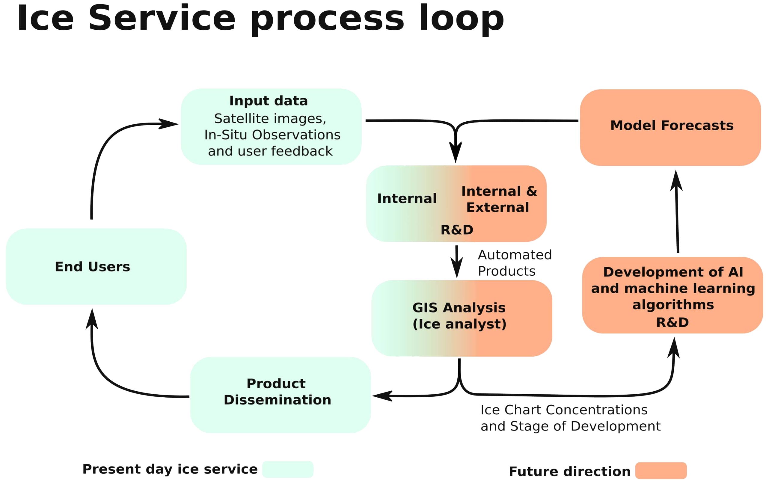
Figure 11. The NIS service process chain currently (green) and the direction for the future (red). The hope is that automated products will provide a more regulatory constrained data format to feed into forecast models and eventually to aid in the creation of model forecasts than what is currently available from hand drawn ice charts. This will be aided by an increase in satellite data availability and in situ observations from increased boat traffic in the region, especially with regards to the NIS hosted Ice Watch program.
Ice analysts possess extensive training and experience in comprehending local conditions, meteorological patterns, and the intricate dynamics of ice drift. These factors present ongoing challenges for automation and modelling in comparison to real-world observations. Looking optimistically toward the future, the vision for ice services is to develop products that incorporate pertinent validation metrics, with input from seasoned ice analysts. Such an approach which will enrich and expand our repository of ice-related information.
Author contributions
WC: Writing – review & editing, Writing – original draft, Investigation, Data curation, Conceptualization. PW: Writing – review & editing, Writing – original draft. NH: Writing – review & editing, Writing – original draft. AE: Writing – review & editing, Writing – original draft. TR: Writing – review & editing, Writing – original draft.
Funding
The author(s) declare that financial support was received for the research, authorship, and/or publication of this article. Funding for this article was received from the Research Council of Norway.
Conflict of interest
The authors declare that the research was conducted in the absence of any commercial or financial relationships that could be construed as a potential conflict of interest.
Publisher’s note
All claims expressed in this article are solely those of the authors and do not necessarily represent those of their affiliated organizations, or those of the publisher, the editors and the reviewers. Any product that may be evaluated in this article, or claim that may be made by its manufacturer, is not guaranteed or endorsed by the publisher.
References
ACSYS. (2003). ACSYS Historical Ice Chart Archive, (1553-2002) (Tromsø, Norway: Arctic Climate System Study). IACPO Informal Report No. 8.
Andersson T. R., Hosking J. S., Pe´rez-Ortiz M., Paige B., Elliott A., Russell C., et al. (2021). Seasonal Arctic sea ice forecasting with probabilistic deep learning. Nat. Commun. 12. doi: 10.1038/s41467-021-25257-4
Arthun M., Onarheim I. H., Dörr J., Eldevik T. (2021). The seasonal and regional transition to an ice-free Arctic. Geophys. Res. Lett. 48, e2020GL090825. doi: 10.1029/2020GL090825
Babb D. G., Galley R. J., Howell S. E. L., Landy J. C., Stroeve J. C., Barber D. G. (2022). Increasing multiyear sea ice loss in the Beaufort sea: A new export pathway for the diminishing multiyear ice cover of the Arctic ocean. Geophys. Res. Lett. 49, e2021GL097595. doi: 10.1029/2021GL097595
Babb D. G., Kirillov S., Galley R. J., Straneo F., Ehn J. K., Howell S. E. L., et al. (2021). Sea ice dynamics in Hudson strait and its impact on winter shipping operations. Journal Geophys. Res.: Oceans 126, e2021JC018024. doi: 10.1029/2021JC018024
Barber D. G., Massom R. A. (2007). “Chapter 1 The Role of Sea Ice in Arctic and Antarctic Polynyas,” in Polynyas: Windows to the World, vol. 74 . Eds. Smith W. O., Barber D. G. (Amsterdam, Netherlands: Elsevier), 1–54. doi: 10.1016/S04229894(06)74001-6
Blair B., Andrea M. U. G., Jelmer J., Steffen M. O., Machiel L. (2022). Mind the gap! A consensus analysis of users and producers on trust in new sea ice information products. Climate Serv. 28, 100323. doi: 10.1016/j.cliser.2022.100323
Blockley E., Vancoppenolle M., Hunke C. Bitz E., Feltham D., Lemieux J., Losch M., et al. (2020). The future of sea ice modeling: where do we go from here?” In. Bull. Am. Meteorol. Soc. 101, E1304–E1311. doi: 10.1175/BAMS-D-20-0073.1
Campbell E. C., Wilson E. A., Moore G. W. K., Riser S. C., Brayton C. E., Mazloff M. R., et al. (2019). Antarctic offshore polynyas linked to Southern Hemisphere climate anomalies. Nature 570, 319–325. doi: 10.1038/s41586-019-1294-0
Canadian Ice Service. (2005). MANICE: Manual of Standard Procedures for Observing and Reporting Ice Conditions. Ninth Edition (Ottawa, Ontario: Crown copyrights reserved. Meteorological Service of Canada). Available at: https://publications.gc.ca/site/eng/9.646757/publication.html. Environment Canada.
Casey J. A., Howell S. E. L., Tivy A., Haas C. (2016). Separability of sea ice types from wide swath C- and L-band synthetic aperture radar imagery acquired during the melt season. Remote Sens. Environ. 174, 314–328. doi: 10.1016/j.rse.2015.12.021
Cheng A., Casati B., Tivy A., Zagon T., Lemieux J.-F., Tremblay L. B. (2020). Accuracy and inter-analyst agreement of visually estimated sea ice concentrations in Canadian ice service ice charts using single-polarization RADARSAT-2. Cryosphere 14, 1289–1310. doi: 10.5194/tc-14-1289-2020
CHNL. (2020). Northern Sea Route Information Office. Available online at: https://arctic-lio.com/.
Dagestad K. F., Röhrs J., Breivik Ø., Ådlandsvik B. (2018). OpenDrift v1. 0: a generic framework for trajectory modelling. Geosci. Model. Dev. 11, 1405–1420. doi: 10.5194/gmd-11-1405-2018
Dawson J., Cook A., Holloway J., Copland L. (2022). “Analysis of Changing Levels of Ice Strengthening (Ice Class) among Vessels Operating in the Canadian Arctic over the Past 30 Years. ARCTIC 75 (4), 413–430. doi: 10.14430/arctic75553
Deggim H. (2018). The international code for ships operating in polar waters (Polar Code). Sustain. shipping changing Arctic, 15–35. doi: 10.1007/978-3-319-78425-0_2
Dierking W. (2013). Sea ice monitoring by synthetic aperture radar. Oceanography 26, 100–111. doi: 10.5670/oceanog
Dierking W. (2020). “Maritime Surveillance with Synthetic Aperture Radar, Sea Ice and Icebergs,” in SAR Handbook: Comprehensive Methodologies for Forest Monitoring and Biomass Estimation. University of Naples Federico II, Naples, Italy: Institution of Engineering and Technology, pp. 173–225. doi: 10.1049/SBRA521E
Dierking W., Iannini L., Davidson M. (2022). “Joint use of L-and C-band spaceborne SAR data for sea ICE monitoring,” in IGARSS 2022 - 2022 IEEE International Geoscience and Remote Sensing Symposium, Kuala Lumpur, Malaysia. 4711–4712. doi: 10.1109/IGARSS46834.2022.9884133
Divine D. V., Dick C. (2006). Historical variability of sea ice edge position in the Nordic Seas. J. Geophys. Res. 111. doi: 10.1029/2004JC002851
Docquier D., Fuentes-Franco R., Koenigk T., Fichefet T. (2020). Sea ice—Ocean interactions in the Barents sea modeled at different resolutions. Front. Earth Sci. 8. doi: 10.3389/feart.2020.00172
Drivenes E.-A. (1994). Adolf Hoel – polar ideologue and imperialist of the Polar Sea. Acta Borealia 11, 63–72. doi: 10.1080/08003839408580437
Eayrs C., Holland D., Francis D., Wagner T., Kumar R., Li X. (2019). Understanding the seasonal cycle of Antarctic sea ice extent in the context of longer-term variability. Rev. Geophys. 57, 1037–1064. doi: 10.1029/2018RG000631
E.U. Copernicus Marine Service Information (CMEMS). (2023). Arctic Ocean - Sea and Ice Surface Temperature. Toulouse, France.
Extreme Earth Project. (2021). Implementation and evaluation of the Polar use case - version II (Extreme Earth Project). Available online at: https://earthanalytics.eu/deliverables.html (Accessed 2024-06-24). Deliverable D5.5.
Færch L., Dierking W., Hughes N., Doulgeris A. P. (2023). A comparison of CFAR object detection algorithms for iceberg identification in L- and C-band SAR imagery of the Labrador sea. Cryosphere Discuss. 2023, 1–26. doi: 10.5194/tc-2023-17
Fox-Kemper B., Adcroft A., Böning C. W., Chassignet E. P., Curchitser E., Danabasoglu G., et al. (2019). Challenges and prospects in ocean circulation models. Front. Mar. Sci. 6. doi: 10.3389/fmars.2019.00065
Haykin S., Lewis E. O., Raney R.K., Rossiter J. R. (1994). Remote sensing of sea ice and icebergs Vol. 13 (Hoboken, New Jersey, USA: John Wiley & Sons).
Heygster G., Hendricks S., Kaleschke L., Maass N., Mills P., Stammer D., et al. (2009). L-Band Radiometry for Sea-Ice Applications, Executive Summary of Final Report for ESA ESTEC Contract 21130/08/NL/EL. Germany: University of Bremen.
Hovelsrud G. K., Olsen J., Nilsson A. E., Kaltenborn B., Lebel J. (2023). Managing Svalbard tourism: inconsistencies and conflicts of interest. Arctic Rev. Law Polit. 14, 86–106. doi: 10.23865/arctic.v14.5113
Hughes N., Qvistgaard K., Seppänen J., Eriksson P., Kangas A., Grönfeldt I., et al. (2020). KEPLER Deliverable Report: Overall Assessment of Stakeholder Needs. Available online at: https://kepler-polar.eu/deliverables/index.html.
Hunke E., Allard R., Blain P., Blockley E., Feltham D., Fichefet T., et al. (2020). Should sea-ice modeling tools designed for climate research be used for short-term forecasting? Curr. Climate Change Rep. 6, 121–136. doi: 10.1007/s40641-020-00162-y
Huntington H. P., Zagorsky A., Kaltenborn B. P., Shin H. C., Dawson J., Lukin M., et al. (2021). Societal implications of a changing Arctic Ocean. Ambio 51 (2), 298–306. doi: 10.1007/s13280-021-01601-2
Ice Watch. (2023). Norwegian Meteorological Institute. Available online at: https://icewatch.met.no/.
Ice Watch ASSIST Data Network, Norwegian Meteorological Institute. (2006). Ice Watch Program for Sea Ice Observations. Available online at: https://icewatch.met.no/ (Accessed January 1st 2024).
International Hydrographic Organization (IHO). (2014). Ice Information Product Specification (Monaco: JCOMM). Tech. rep. S-411.
International Maritime Organization. (1974). International Convention for the Safety of Life At Sea (United Kingdom: International Maritime Organization). Available at: https://www.refworld.org/legal/agreements/imo/1974/en/46856.
Jakobsson M., Grantz A., Kristoffersen Y., Macnab R. (2003). Physiographic provinces of the Arctic Ocean seafloor. Geol. Soc. America Bull. 115, 1443–1455. doi: 10.1130/B25216.1
Jakobsson M., Mayer L. A., Coakley B., Dowdeswell J. A., Forbes S., Fridman B. E., et al. (2012). The international bathymetric chart of the Arctic ocean (IBCAO) version 3.0. Geophys. Res. Lett. 39. doi: 10.1029/2012GL052219
JCOMM Expert Team on Sea Ice. (2014). SIGRID-3: a vector archive format for sea ice georeferenced information and data. Version 3.0. JCOMM Technical Report 23 (Geneva, Switzerland: WMO & IOC), 40. doi: 10.25607/OBP-1498.2
Jeuring J., Knol-Kauffman M. (2019). Mapping Weather, Water, Ice and Climate Knowledge & Information Needs for Maritime Activities in the Arctic Survey report. Available online at: https://salienseas.com/wp-content/uploads/2019/09/SALIENSEAS-Mapping-WWICKnowledge-and-Information-Needs-for-Maritime-Activities-in-the-Arctic_FINAL_20190830.pdf.
Jeuring J., Knol-Kauffman M., Sivle A. (2019). Toward valuable weather and sea-ice services for the marine Arctic: exploring user–producer interfaces of the Norwegian Meteorological Institute. Polar Geogr. 43, 139–159. doi: 10.1080/1088937x.2019.1679270
Jung T., Gordon N. D., Bauer P., Bromwich D. H., Chevallier M., Day J. J., et al. (2016). Advancing polar prediction capabilities on daily to seasonal time scales. Bull. Am. Meteorol. Soc. 97, 1631–1647. doi: 10.1175/BAMS-D-14-00246.1
Kangas A., Seppa¨nen J., Eriksson P., Grönfeldt I., Wagner P., Hughes N., et al. (2020). KEPLER Deliverable Report: Harmonisation and improvement of sea ice mapping products (Finnish Meteorological Institute Finnish Ice Service). Available at: https://keplerpolar.eu/deliverables/index.html.
Karmakar C., Dumitru C. O., Hughes N., Datcu M. (2023). A visualization framework for unsupervised analysis of latent structures in SAR image time series. IEEE J. Select. Topics Appl. Earth Observ. Remote Sens. 16, 5355–5373. doi: 10.1109/JSTARS.2023.3273122
Karvonen J., Vainio J., Marnela M., Eriksson P., Niskanen T. (2015). A comparison between high-resolution EO-based and ice analyst-assigned sea ice concentrations. IEEE J. Select. Topics Appl. Earth Observ. Remote Sens. 8, 1–9. doi: 10.1109/JSTARS.4609443
KEPLER Project (2020). Key Environmental Monitoring for Polar Latitudes and Environmental Readiness. Available online at: https://kepler-polar.eu/deliverables/ (Accessed 2024-06-24).
Kern S. (2009). Wintertime Antarctic coastal polynya area: 1992–2008. Geophys. Res. Lett. 36. doi: 10.1029/2009GL038062
Khachatrian E., Chlaily S., Eltoft T., Dierking W., Dinessen F., Marinoni A. (2021). Automatic selection of relevant attributes for multi-sensor remote sensing analysis: A case study on sea ice classification. IEEE J. Select. Topics Appl. Earth Observ. Remote Sens. 14, 9025–9037. doi: 10.1109/JSTARS.2021.3099398
Khachatrian E., Dierking W., Chlaily S., Eltoft T., Dinessen F., Hughes N., et al. (2023). SAR and passive microwave fusion scheme: A test case on sentinel-1/AMSR-2 for sea ice classification. Geophys. Res. Lett. 50, e2022GL102083. doi: 10.1029/2022GL102083
Kim Y. H., Min S. K., Gillett N. P., Notz D., Malinina E. (2023). Observationally constrained projections of an ice-free Arctic even under a low emission scenario. Nat. Commun. 14, 3139. doi: 10.1038/s41467-023-38511-8
Koenigk T., Mikolajewicz U., Jungclaus J. H., Kroll A. (2008). Sea ice in the Barents Sea: seasonal to interannual variability and climate feedbacks in a global coupled model. Climate Dynam. 32, 1119–1138. doi: 10.1007/s00382008-0450-2
Krumpen T., Gerdes R., Haas C., Hendricks S., Herber A., Selyuzhenok V., et al. (2016). Recent summer sea ice thickness surveys in Fram Strait and associated ice volume fluxes. Cryosphere 10, 523–534. doi: 10.5194/tc-10-523-2016
Kubat I., Sayed M., Savage S. B., Carrieres T. (2005). An operational model of iceberg drift”. Int. J. Offshore Polar Eng. 15, 26–30.
Kvanum A. F., Palerme C., Müller M., Rabault J., Hughes N. (2024). Developing a deep learning forecasting system for short-term and high-resolution prediction of sea ice concentration. doi: 10.5194/egusphere-2023-3107
Landy J., Bouffard J., Wilson C., Rynders S., Aksenov Y., Tsamados M. (2021). Improved arctic sea ice freeboard retrieval from satellite altimetry using optimized sea surface decorrelation scales. J. Geophys. Res.: Oceans 126, e2021JC017466. doi: 10.1029/2021JC017466
Laroche S., Poan E. (2021). Impact of the arctic observing systems on the ECCC global weather forecasts. Q. J. R. Meteorol. Soc. 148, 252–271. doi: 10.1002/qj.4203
Lawrence H., Bormann N., Sandu I., Day J., Farnan J., Bauer P. (2019). Use and impact of Arctic observations in the ECMWF Numerical Weather Prediction system. Q. J. R. Meteorol. Soc. 145, 3432–3454. doi: 10.1002/qj.3628
Lima R., Vahedi B., Hughes N., Barrett A. P., Meier W., Karimzadeh M. (2023). Enhancing sea ice segmentation in Sentinel-1 images with atrous convolutions. Int. J. Remote Sens. 44, 5344–5374. doi: 10.1080/01431161.2023.2248560
Lohse J., Doulgeris A. P., Dierking W. (2020). Mapping sea-ice types from Sentinel-1 considering the surface-type dependent effect of incidence angle. Ann. Glaciol. 61, 260–270. doi: 10.1017/aog.2020.45
Løset S., Carstens T. (1996). Sea ice and iceberg observations in the western Barents sea in 1987. Cold Reg. Sci. Technol. 24, 323–340. doi: 10.1016/0165-232X(95)00029-B
Lundesgaard Ø., Sundfjord A., Renner A. H. H. (2021). Drivers of interannual sea ice concentration variability in the Atlantic water inflow region North of Svalbard. J. Geophys. Res. Oceans 126, e2020JC016522. doi: 10.1029/2020JC016522
Luo B., Luo D., Ge Y. (2023). Origins of Barents-Kara sea-ice interannual variability modulated by the Atlantic pathway of El Niño–Southern oscillation. Nat. Commun. 14, 585. doi: 10.1038/s41467-023-36136-5
Mallet P. E., Claud C., Vicomte M. (2017). North Atlantic polar lows and weather regimes: do current links persist in a warmer climate? Atmos. Sci. Lett. 18, 349–355. doi: 10.1002/asl.763
Marchenko N., Borch O. J., Markov S. V., Andreassen N. (2015). “Maritime activity in the high north - The range of unwanted incidents and risk patterns”,” in Proceedings International Conference on Port and Ocean Engineering under Arctic Conditions 2015, Trondheim, Norway.
Massonnet F., Fichefet T., Goosse H., Bitz C. M., Philippon-Berthier G., Holland M. M., et al. (2012). Constraining projections of summer Arctic sea ice. Cryosphere 6, 1383–1394. doi: 10.5194/tc-6-1383-2012
Matveeva T. A., Semenov V. A. (2022). Regional features of the Arctic sea ice area changes in 2000-2019 versus 1979-1999 periods. Atmosphere 13, 2073–4433. doi: 10.3390/atmos13091434
Meier W. N., Stroeve J. (2022). An updated assessment of the changing Arctic sea ice cover. Oceanography 35, 10–19. doi: 10.5670/oceanog
Meleshko V. P., Pavlova T., Bobylev L. P., Golubkin P. (2020). Current and projected sea ice in the Arctic in the twenty-first century. Sea Ice Arctic: Past present Future, 399–463. doi: 10.1007/978-3-030-21301-5_10
Melsheimer C., Spreen G. (2022). Remote sensing of multiyear ice in the Antarctic. DAC H2022. Leipzig Deutschland , 21–25. doi: 10.5194/dach2022-284
Metzger E. J., Helber R. W., Hogan P. J., Posey P. G., Thoppil P. G., Townsend T. L., et al. (2017). Global Ocean Forecast System 3.1 Validation Testing (Naval Research Laboratory, Stennis Space Center, MS). Tech. rep. NRL/MR/7320–17-9722. Approved for public release; distribution is unlimited.
Mioduszewski J. R., Vavrus S., Wang M., Holland M., Landrum L. (2019). Past and future interannual variability in Arctic sea ice in coupled climate models. Cryosphere 13, 113–124. doi: 10.5194/tc-13-113-2019
Mö N.-A., Solheim J.-E., Humlum O., Falk-Petersen S. (2020). Changes in Barents Sea ice Edge Positions in the Last 440 years: A Review of Possible Driving Forces. Int. J. Astronom. Astrophys. 10, 97–164. doi: 10.4236/ijaa.2020.102008
Moen M. A., Doulgeris A. P., Anfinsen S. N., Renner A. H., Hughes N., Gerland S., et al. (2013). Comparison of feature based segmentation of full polarimetric SAR satellite sea ice images with manually drawn ice charts. Cryosphere 7, 1693–1705. doi: 10.5194/tc-7-1693-2013
Müller M., Batrak Y., Dinessen F., Grote R., Wang K. (2023). Challenges in the description of sea ice for a kilometer-scale weather forecasting system. Weather Forecast. 38, 1157–1171. doi: 10.1175/WAF-D-22-0134.1
Murphy D. L., Cass J. L. (2012). The international ice patrol: safeguarding life and property at sea”. Coast. Guard J. Saf. Secur. at Sea 69.
Mustonen T., Mustonen K., Saijets J., Feodoroff P., Kirillov J., Mikaelsson S., et al. (2019). Report on Deliverable D1.2: Community-Based Observation and Societal Needs (EU Project Kepler, Work Package Report). Available at: https://kepler-polar.eu/deliverables/index.html.
National Snow and Ice Data Center. (2024). International Ice Charting Working Group. Available online at: https://nsidc.org/noaa/iicwg (Accessed 2024).
Nesterov A. V., Gavrilov Y. G., Buzin I. V., Skutin A. A., Gudoshnikov Y. P., Kornishin K. A., et al. (2023). “Icebergs detection and characterization capabilities: field trials in the Arctic seas,” in 33rd International Ocean and Polar Engineering Conference, Ottawa, Canada: International Society of Offshore and Polar Engineers. doi: 10.17736/10535381
Onarheim I. H., Årthun M. (2017). Toward an ice-free Barents sea. Geophys. Res. Lett. 44, 8387–8395. doi: 10.1002/2017GL074304
Onarheim I. H., Eldevik T., Smedsrud L. H., Stroeve J. C. (2018). Seasonal and regional manifestation of Arctic sea ice loss. J. Climate 31, 4917–4932. doi: 10.1175/JCLI-D-17-0427.1
Overland J. E., Wang M. (2013). When will the summer Arctic be nearly sea ice free? Geophys. Res. Lett. 40, 2097–2101. doi: 10.1002/grl.50316
Parsons J., Progoulaki M. (2014). “Promoting safety and managing risks in arctic marine transportation: A best practices approach and the polar code,” in Proceedings of the ASME 2014 33rd International Conference on Ocean, Offshore and Arctic Engineering. San Francisco, California, USA: American Society of Mechanical Engineers (ASME). doi: 10.1115/OMAE2014-23271
Posey P., Metzger E., Wallcraft A., Hebert D., Allard R., Smedstad O., et al. (2015). Improving arctic sea ice edge forecasts by assimilating high horizontal resolution sea ice concentration data into the US navy’s ice forecast systems. Cryosphere 9, 1735–1745. doi: 10.5194/tc-9-1735-2015
QGIS Development Team. (2023). QGIS Geographic Information System. Open Source Geospatial Foundation Project. Version 3.22. Available at: https://qgis.org [Accessed 20 September 2023].
Regan H., Rampal P., Ólason E., Boutin G., Korosov A. (2023). Modelling the evolution of Arctic multiyear sea ice over 2000–2018. Cryosphere 17, 1873–1893. doi: 10.5194/tc-17-1873-2023
Renner A. H. H., Hendricks S., Gerland S., Beckers J., Haas C., Krumpen T. (2013). Large-scale ice thickness distribution of first-year sea ice in spring and summer north of Svalbard. Ann. Glaciol. 54, 13–18. doi: 10.3189/2013AoG62A146
Röhrs J., Gusdal Y., Rikardsen E. S. U., Durán Moro M., Brændshøi J., Kristensen N. M., et al. (2023). Barents-2.5km v2.0: an operational data-assimilative coupled ocean and sea ice ensemble prediction model for the Barents Sea and Svalbard. Geosci. Model. Dev. 16, 5401–5426. doi: 10.5194/gmd-16-5401-2023
Rojo M., Claud C., Mallet P.-E., Noer G., Carleton A. M., Vicomte M. (2015). Polar low tracks over the Nordic Seas: a 14-winter climatic analysis. Tellus A: Dynam. Meteorol. Oceanogr. 67 (1), 24660. doi: 10.3402/tellusa.v67.24660
Russian Maritime Register of Shipping (2024). Russian Maritime Register of Shipping. Available online at: https://rs-class.org/en/.
Salvó C. S., Gomez Saez L., Arce J. C. (2023). Multi-band SAR intercomparison study in the Antarctic Peninsula for sea ice and iceberg detection. Front. Mar. Sci. 10, 1255425. doi: 10.3389/fmars.2023.1255425
Sandven S., Spreen G., Georg H., Girard-Ardhuin F., Farrell S. L., Dierking W., et al. (2023). Sea ice remote sensing—Recent developments in methods and climate data sets. Surv. Geophys. 44, 1653–1689. doi: 10.1007/s10712-023-09781-0
Scardilli A. S., Salvó C. S., Saez L. G. (2022). Southern Ocean ice charts at the Argentinian Naval Hydrographic Service and their impact on safety of navigation. Front. Mar. Sci. 9. doi: 10.3389/fmars.2022.971894
Sea Ice, JCOMM Expert Team on. (2014). sea-ice nomenclature: Snapshot of the WMO sea ice nomenclature WMO No. 259, volume1–terminology and codes; volume II–illustrated glossary and III–international system of sea-ice symbols.
Serreze M. C., Meier W. N. (2018). The Arctic’s sea ice cover: trends, variability, predictability, and comparisons to the Antarctic. Ann. New York Acad. Sci. 1436, 36–53. doi: 10.1111/nyas.13856
Serreze M. C., Stroeve J. (2015). Arctic sea ice trends, variability and implications for seasonal ice forecasting. Phil. Trans. R. Soc A 373, 20140159. doi: 10.1098/rsta.2014.0159
Shi Q., Yang Q., Mu L., Wang J., Massonnet F., Mazloff M. R. (2021). Evaluation of sea-ice thickness from four reanalyses in the Antarctic Weddell Sea. Cryosphere 15, 31–47. doi: 10.5194/tc-15-31-2021
Shuchman R. A., Onstott R. G., Johannessen O. M., Sandven S., Johannessen J. A. (2004). Processes at the ice edge: the arctic”. Synth. Aperture Radar Mar. user’s manual, 373–395.
Singha S., Johansson M., Hughes N. F., Hvidegaard S. M., Skourup H. (2018). Arctic sea ice characterization using spaceborne fully polarimetric L-, C-, and X-band SAR with validation by airborne measurements. IEEE Trans Geosci Remote Sens. 56, 3715–3734. doi: 10.1109/TGRS.36
Smith G. C., Allard R., Babin M., Bertino L., Chevallier M., Corlett G., et al. (2019). Polar ocean observations: A critical gap in the observing system and its effect on environmental predictions from hours to a season. Front. Mar. Sci. 6. doi: 10.3389/fmars.2019.00429
Spreen G., Kaleschke L., Heygster G. (2008). Sea ice remote sensing using AMSR-E 89-GHz channels”. J. Geophys. Res. 113. doi: 10.1029/2005JC003384
Stewart E. J., Liggett D., Lamers M., Ljubicic G., Dawson J., Thoman R., et al. (2019). Characterizing polar mobilities to understand the role of weather, water, ice and climate (WWIC) information. Polar Geogr. 43, 95–119. doi: 10.1080/1088937X.2019.1707319
Stocker A. N., Renner A. H. H., Knol-Kauffman M. (2020). Sea ice variability and maritime activity around Svalbard in the period 2012-2019. Sci. Rep. 10, 17043. doi: 10.1038/s41598-020-74064-2
Sumata H., de Steur L., Divine D. V. (2023). Regime shift in Arctic ocean sea ice thickness. Nature 615, 443–449. doi: 10.1038/s41586-022-05686-x
Tietsche S., Mueller M., Bertino L., Garric G., Goessling H., Pedersen L. T., et al. (2020). KEPLER Deliverable Report: Recommendations for more user-relevant sea-ice forecasts (European Centre for Medium-Range Weather Forecasts (ECMWF). Available at: https://kepler-polar.eu/deliverables/index.html.
Tilling R. L., Ridout A., Shepherd A. (2018). Estimating Arctic sea ice thickness and volume using CryoSat-2 radar altimeter data. Adv. Space Res. 62, 1203–1225. doi: 10.1016/j.asr.2017.10.051
Turner J., Guarino M. V., Arnatt J., Jena B., Marshall G. J., Phillips T., et al. (2020). Recent decrease of summer sea ice in the Weddell sea, Antarctica. Geophys. Res. Lett. 47, e2020GL087127. doi: 10.1029/2020GL087127
U.S. National Ice Center. (2024). (U.S. National Ice Center). Available online at: https://usicecenter.gov/ (Accessed 05 March 2024).
Veland S., Wagner P., Bailey D., Everett A., Goldstein M., Rivas H. R., et al. (2021). Knowledge needs in sea ice forecasting for navigation in Svalbard and the High Arctic. doi: 10.13140/RG.2.2.11169.33129
Wadhams P. (2000). Ice in the Ocean. 1st (Boca Raton, Florida, USA: CRC Press/ Taylor and Francis Group). doi: 10.1201/9781482283082
Wagner P. M., Hegelund O. J. (2020). Key Environmental Monitoring for Polar Latitudes and Environmental Readiness. Available online at: https://kepler-polar.eu/deliverables/.
Wagner P. M., Hegelund O. J., Hughes N., Qvistgaard K., Seppänen J., Eriksson P., et al. (2019). Report on Deliverable D1.1: Stakeholder Needs: Maritime Sector Needs (Norwegian Meteorological Institute - Norwegian Ice Service). Available at: https://kepler-polar.eu/deliverables/index.html.
Wagner P. M., Hughes N., Bourbonnais P., Stroeve J., Rabenstein L., Bhatt U., et al. (2020). Sea-ice information and forecast needs for industry maritime stakeholders. Polar Geogr. 43, 160–187. doi: 10.1080/1088937X.2020.1766592
Williams T., Korosov A., Rampal P., Olasoń E. (2021). Presentation and evaluation of the Arctic sea ice forecasting system neXtSIM-F. Cryosphere 15, 3207–3227. doi: 10.5194/tc-15-3207-2021
WMO. (2004). Ice chart colour code standard - 259. Available online at: https://library.wmo.int/records/item/37175-ice-chart-colourcode-standard.
Keywords: sea ice (Arctic), Arctic, Norway, Svalbard, Barents, Fram Strait, Ice Service, sea ice operations
Citation: Copeland W, Wagner P, Hughes N, Everett A and Robertsen T (2024) The MET Norway Ice Service: a comprehensive review of the historical and future evolution, ice chart creation, and end user interaction within METAREA XIX. Front. Mar. Sci. 11:1400479. doi: 10.3389/fmars.2024.1400479
Received: 13 March 2024; Accepted: 10 July 2024;
Published: 08 August 2024.
Edited by:
Kum Fai Yuen, Nanyang Technological University, SingaporeReviewed by:
Leandro Ponsoni, Flanders Marine Institute, BelgiumJan L. Lieser, Bureau of Meteorology, Australia
Copyright © 2024 Copeland, Wagner, Hughes, Everett and Robertsen. This is an open-access article distributed under the terms of the Creative Commons Attribution License (CC BY). The use, distribution or reproduction in other forums is permitted, provided the original author(s) and the copyright owner(s) are credited and that the original publication in this journal is cited, in accordance with accepted academic practice. No use, distribution or reproduction is permitted which does not comply with these terms.
*Correspondence: William Copeland, d2lsbGlhbWpwQG1ldC5ubw==