Subsurface temperature estimation of mesoscale eddies in the Northwest Pacific Ocean from satellite observations using a residual muti-channel attention convolution network

The mesoscale eddies are prevalent oceanic circulation phenomena, exerting significant influence on various aspects of the marine environment including energy transfer, material transport and ecosystem dynamics in the Northwest Pacific Ocean. However, due to sparse vertical observational data, the understanding of the three-dimensional temperature structure of individual cases of mesoscale eddies remains limited. In recent years, utilizing surface remote sensing observations to estimate subsurface temperature anomaly has been crucial for comprehending the intricate multi-dimensional dynamic processes in the ocean. Consequently, this paper proposes an eddy residual multi-channel attention convolution network (ERCACN) with the adaptive threshold and designs the combination of various surface features to estimate the eddy subsurface temperature anomaly (ESTA). By integrating results with climatic temperature, thermal structures containing 46 levels at depths up to 1000 m could be obtained, achieving excellent daily temporal resolution and 0.25° spatial resolution. Validation using independent Argo profiles from 2016 to 2017 reveals that the combination of multiple surface variables outperforms univariate methods, and the ERCACN model demonstrates superior performance compared to other approaches. Overall, with an 8% error deemed acceptable, the ERCACN model achieves a precision of 88.08% in estimating ESTA. This method provides a novel perspective for other essential oceanic variables, contributing to a better perception of the global climate system.

1 Introduction

Mesoscale eddies are widely distributed in the global oceans, with the horizontal radius primarily ranging from 50 km to 300 km and vertical depths exceeding 1000 m (Chelton et al., 2011a; Dong et al., 2014; Zhang et al., 2014b; Li et al., 2024). They play crucial roles in the mid- to long-distance water mass exchange, material and energy transport, and vertical dynamic enhancement (Liu and Tang, 2018; Chen et al., 2023b). As one of the most complex regions in the ocean circulation system, the Northwest Pacific Ocean has a significant number of mesoscale eddies, exerting profound impacts on the distribution of temperature, salinity, and chlorophyll (Xu et al., 2016; Dong et al., 2017; Sun et al., 2022; Yuan and Hu, 2023). For instance, mesoscale eddies induce heat flux anomalies at the sea surface, weakening the upper ocean thermal structure in the Kuroshio Extension region, resulting in a notable decrease in the sea surface temperature (SST) and corresponding reductions in vertical heat transfer (Yang et al., 2018; Shan et al., 2020). In addition, mesoscale eddies alter the reproductive patterns and migration behaviors of marine organisms by influencing nutrient redistribution (Bibby et al., 2008; Dobashi et al., 2022; Ueno et al., 2023; An et al., 2024). Previous studies have investigated the horizontal structure, lifetime, and trajectories of mesoscale eddies through the comprehensive integration of multi-source data, aiming to elucidate their complex impacts on various physical dynamic processes in the marine environment (Chelton et al., 2011b; Yang et al., 2013; Dong et al., 2022).

During the development of satellite sensors, ocean surface data with high spatiotemporal resolution can be continuously obtained, providing abundant information for researching mesoscale eddy surface features (Zhao et al., 2021; Huo et al., 2024). However, due to the lack of high-resolution in-situ observational data, our understanding of the generation and dissipation mechanisms of the vertical three-dimensional temperature structure of specific mesoscale eddies remains limited (Zhang et al., 2016; Chen et al., 2023b). Zhang et al. (2013) utilized satellite sea surface information and Argo float-measured data to obtain the universal structure of mesoscale eddies by normalization method and composite analyses. Zhang et al. (2014a) combined high-resolution satellite altimeter data with temperature-salinity data observed by Argo to reconstruct the potential density field of mesoscale eddies and estimated the volume transport of water masses through comprehensive analysis methods. Nencioli et al. (2018) reconstructed the specific three-dimensional structure of mesoscale eddies using similar methods and studied the transport and exchange of water masses. Yang et al. (2019) analyzed the horizontal and vertical heat and salinity transport caused by mesoscale eddies by combining observation data, satellite data, and ocean model data. Considering the influence of eddy currents and background flows, He et al. (2021) enhanced the universal three-dimensional reconstruction of mesoscale eddies and explored their role in the redistribution of water masses and heat transfer. Despite the increase in various in-situ observational data over time, the impact of uneven spatial distribution and long data collection period still exists. Previous studies have mainly focused on the mean three-dimensional structure of eddies or conducted composite analyses of individual eddies. However, it remains challenging to acquire continuous and high-resolution three-dimensional temperature structures of different specific mesoscale eddies in the Northwest Pacific Ocean. In addition, the temperature structure of mesoscale eddies exerts profound ecological impacts, influencing the distribution of heat and nutrients within oceanic regions (Shan et al., 2020). The magnitude and direction of heat fluxes can be quantified more effectively with the accurate temperature structure of mesoscale eddies, thereby refining global climate models and predictions. Moreover, understanding how temperature gradients impact particle advection and diffusion can aid in predicting pollutant dispersal, tracking the migration patterns of marine species, and assessing ecosystem resilience to environmental changes (Ueno et al., 2023). Next, variations in temperature structure can alter marine organism metabolic rates, reproductive cycles, and habitat preferences, ultimately influencing marine ecosystem composition and function (An et al., 2024). Clarifying the thermal characteristics of mesoscale eddies can contribute to predicting species distributions, evaluating habitat suitability, and informing marine conservation strategies. Therefore, estimating the continuous and high-resolution temperature structure of mesoscale eddies holds significant scientific and practical implications.

Currently, the combination of various satellite ocean surface data and Argo profiles constitutes an effective method for accurately estimating the subsurface three-dimensional temperature structure (Chen et al., 2023d; Chen et al., 2024). Firstly, relatively straightforward univariate or multivariate linear regression (MLR) is one of the most common approaches. For instance, Guinehut et al. (2012) described the temperature field at a spatial resolution of 1° for the period from 1993 to 2009 by combining satellite observations of sea level anomaly (SLA) and SST data with Argo profiles using the MLR method. Jeong et al. (2019) also utilized the MLR approach to estimate the subsurface temperature structure by incorporating SLA, SST anomaly (SSTA), wind stress anomaly and Argo observational data. In addition, a combination of dynamic and statistical methods has been applied to reconstruct the three-dimensional temperature structure. Yan et al. (2020) estimated the subsurface density field using an improved surface quasi-geostrophic method with sea surface height (SSH) and sea surface density (SSD) data, and the ocean temperature field can be achieved by applying the least squares multivariate algorithm combined with SST and sea surface salinity (SSS) data. In recent years, significant advancements have been made in the inversion of the three-dimensional temperature structure using artificial intelligence methods. Ali et al. (2004) employed artificial neural networks, integrating various sea surface information including SST, SSH, and sea surface wind (SSW) to estimate the temperature structure in the Arabian Sea. Wu et al. (2012) reconstructed the temperature anomaly of the North Atlantic at a spatial resolution of 1° using a self-organizing map neural network approach with SSH anomaly (SSHA), SSTA and SSS anomaly (SSSA). Lu et al. (2019) partitioned and predicted temperature fields in different regions of the global ocean by combining pre-clustering and neural networks, demonstrating better performance compared to methods without pre-clustering. Xie et al. (2022) estimated the ocean temperature field at a spatial resolution of 0.5° by applying an improved U-net network with satellite data including SLA, SSW, SST, wind stress curl and Argo profiles. Chen et al. (2023a) proposed an algorithm combining deep evidence regression networks with empirical orthogonal functions to reconstruct global ocean temperature profiles using sea surface information and Argo observational data. Various machine learning methods have also been applied to estimate the subsurface temperature structure, including the random forest regression (RFR) (Su et al., 2018), support vector machine (Su et al., 2015), multilayer perceptron network (Sammartino et al., 2020), extreme gradient boosting (Su et al., 2019) and convolutional neural network (CNN) (Su et al., 2021). These demonstrate the feasibility of utilizing multiple sea surface information and observational data to estimate subsurface three-dimensional temperature fields.

However, compared to the estimation of temperature profiles in the global ocean, mesoscale eddies exhibit more intricate three-dimensional structures, diverse shapes and pronounced nonlinearity (McGillicuddy, 2016). Yu et al. (2021) devised a method applying the Eddy CNN method for ESTA with SLA and Argo observational profiles. But this network relies on SLA alone, which contains limited surface feature information, and the relatively simplistic structure of Eddy CNN poses challenges in dynamically adjusting attention weights and reducing noise to capture mesoscale eddy features. In addition, SST and SSW play pivotal roles in the lifecycle of mesoscale eddies. Hence, this study proposes an effective combination of various remote sensing features, including SLA, SSTA, SSW speed anomaly (SSWSA), and its u and v components (referred to as UWA and VWA, respectively), and designs the ERCACN method with the adaptive threshold for residual multi-channel attention module. Integrating Argo observational data, this algorithm adopts a data-driven approach to bypass complex physical modeling, aiming to efficiently estimate the three-dimensional temperature structure of mesoscale eddies in the Northwest Pacific Ocean with a spatial resolution of 0.25° and a temporal resolution of 1 day, reaching depths of up to 1000 m across 46 levels vertically. Section 2 introduces the used satellite observational data, mesoscale eddy data, Argo observational data and climatological data in the study area. Section 3 elaborates on the architecture and configuration of the ERCACN algorithm model. Section 4 discusses the comparative performance of the ERCACN algorithm with other methods in estimating ESTA in the Northwest Pacific Ocean, which demonstrates the effectiveness in temperature estimation for anticyclonic and cyclonic eddies at various depths and different time. Finally, section 5 presents the conclusions.

2 Materials

2.1 Satellite data

Various satellite data products, containing SLA, SSTA, SSWSA, UWA and VWA, are applied for a more effective estimation of ESTA. A gridded SLA with a spatial resolution of 0.25°, named SEALEVEL_GLO_PHY_L4_MY_008_047 and produced by Ssalto/Duacs, is available for free download from the Copernicus Marine and Environmental Monitoring Service (Capet et al., 2014). Subsequently, the 0.25° resolution SSTA data used is derived from the Optimum Interpolation SST (OISST) product, developed by the National Oceanic and Atmospheric Administration (NOAA). OISST v2.1 integrates data from ships, buoys, satellites, and Argo floats using optimal interpolation methods (Huang et al., 2021). The surface wind field is obtained from gridded data provided by the Cross-Calibrated Multi-Platform (CCMP) product, which utilizes a variational analysis method to merge data from multiple microwave radiometers and scatterometers (Mears et al., 2019). SSWSA is computed by subtracting the monthly average wind speed magnitude from the current-day wind field velocity. Similarly, UWA and VWA are also acquired.

2.2 Mesoscale eddy trajectory dataset

The dataset of mesoscale eddy trajectories is extracted from daily gridded sea-surface height anomaly data produced by two satellites, initially provided by the Archiving, Validation, and Interpretation of Satellite Oceanographic (AVISO+) (Chen et al., 2023c). The dataset contains information about the position, amplitude, radius, and temporal evolution of mesoscale eddies. The algorithm identifies mesoscale eddies characterized by connected pixels, with a diameter ranging from 100 to 300 km, an amplitude exceeding 1 cm and a lifespan exceeding 4 weeks (Chelton et al., 2011b). The selected data ranges from 2001 to 2017, with a temporal resolution of 1 day and a spatial resolution of 0.25°.

2.3 Argo data

This article utilizes Argo data obtained from French Research Institute for the Exploitation of the Seas (IFREMER), a well-established global dataset (Wang and Liu, 2024). Figures 1A, B illustrate all the selected Argo profiles that have undergone quality control. The study area is defined as the region between 0° ~ 60° N and 105° ~ 165° E. The downloaded dataset spans 17 years from 2001 to 2017. Before utilizing the Argo data, a comprehensive quality control process was conducted to ensure data reliability (Pun et al., 2014). The Argo data encompass a wide range of parameters, including the initial temperature data points recorded in the Argo profiles, minimum depths observed, minimum number of effective observations, and maximum depth and minimum temperature differences. The detailed quality assurance process for Argo profiles is outlined in Table 1. Initially, the eddy center, size, time and location for mesoscale eddies within the study region are obtained from the eddy dataset. Subsequently, Argo profile locations must fall within the eddy center and radius regions of any identified eddy to filter the appropriate Argo profiles. Then, Argo profiles from 2001 to 2015 are utilized for training ERCACN. Subsequently, the accuracy of the ERCACN method is verified by using Argo profile data from 2016 and 2017.

Figure 1

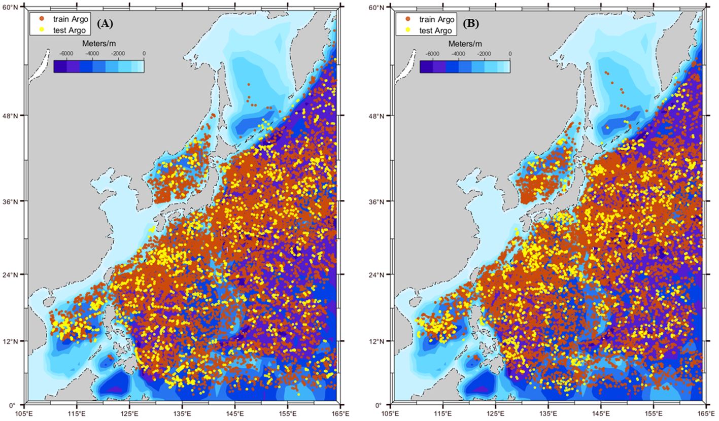
Figure 1 The distribution of selected and quality-controlled Argo locations from 2001 to 2017. (A) Argo observations of anticyclonic eddies; (B) Argo observations of cyclonic eddies. The blue area indicates water depth, the red points denote the locations of Argo used from 2001 to 2015 for the training dataset, and the yellow points represent the locations of Argo selected from 2016 to 2017 for the testing dataset.

Table 1

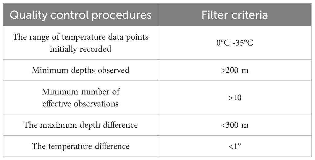
Table 1 The detailed quality assurance process for Argo profiles.

2.4 Climate state data

This study utilizes historical temperature and salinity data from the World Ocean Atlas 2018 (WOA18). The WOA18 calculates the 10-year average climate fields from 1955 to 2017, which serves as a standard for objective analysis (Purkiani et al., 2022). Each average field includes a large amount of observation data, with a high spatial resolution of 0.25°and vertical resolution of 0–5500 m with 102 levels, including 47 levels above 1000 m. The data has been smoothed and mesoscale signals are significantly suppressed, making it suitable for testing the anomalous temperature and salinity structures caused by mesoscale processes as a background field. In this paper, WOA18 temperature data from 5 to 1000 m, comprising 46 levels, are utilized for model training. Meanwhile, to ensure the accuracy of observations in ocean temperature and salinity profiles, CTD sensors equipped on Argo cease operation when ascending to a depth of approximately 5 m from the ocean surface to avoid interference caused by floating debris. This limitation results in Argo’s ability to observe depths ranging from roughly 5 to 10 m from the ocean surface. Therefore, daily SST with a spatial resolution of 0.25°from the OISST data product is used as a substitute to complete the analysis of the thermal structure of eddies.

The temperature anomaly $Y_{a(lon,lat,level)}$ is calculated by subtracting the climatological temperature of WOA18 from the temperature measured by the Argo profiles near the eddy, which indicates the deviation of the point’s temperature from the inter-annual average temperature. Subsequently, this temperature anomaly value at the given location is used as the label variable for training. The Equation 1 is presented below:

$\begin{array}{ll}{Y}_{a(lon,lat,level)}=Y_{Argo(lon,lat,level)}-Y_{WOA(lon,lat,level),}& (1)\end{array}$

where $Y_{Argo(lon,lat,level)}$ represents the temperature measurements of various levels at the longitudinal and latitudinal positions of eddies from Argo observations, and $Y_{WOA(lon,lat,level)}$ denotes the temperature data at corresponding positions from the WOA18.

3 Methods

3.1 Eddy residual muti-channel attention convolution network

3.1.1 The residual module

The CNN model is particularly applied to handle data with grid-like structures, such as images and videos. Features are extracted by using convolutional kernels to local regions of input data, and the spatial dimensions and quantity of feature maps are gradually refined through stacked layers of convolutional and pooling operations. The residual network is introduced to maintain smooth gradient flow and enhance generalization capabilities by incorporating skip connections between network layers (Shankar Manche et al., 2024). This structure effectively mitigates gradient dispersion and explosion during backpropagation optimization. The residual connections enhance the smooth propagation of feature information, ensuring the expressive capability of output feature maps and improving the network’s receptive field without altering the output feature maps. The residual connection method has found broad applications in diverse domains such as ocean temperature reconstruction and image recognition, achieving satisfactory results (Ping et al., 2021; Mahaur et al., 2023). To effectively utilize information from multiple satellite signals and achieve a real-time, stable and efficient estimation of ESTA, we have designed and improved this structure by incorporating various activation functions and modifying the network structure at different layers.

3.1.2 The residual multi-channel attention module with the adaptive threshold

The attention mechanism (Shi et al., 2022; Zhao et al., 2022) has been a hot topic of research in recent years, with the squeeze-and-excitation network (SENet) being recognized as a classic attention algorithm (Zhao et al., 2023). Figure 2 illustrates the architecture of the traditional SENet. Initially, the input feature map h×w×c is processed by the convolution layer and global average pooling (GAP) $F_{sq}(x_c)$ operations to derive a global information feature vector for each channel, resulting in the feature map with a size of 1×1×c as shown in Equation 2. Subsequently, the features map is performed by connecting two fully connected (FC) layers to establish the correlation between different channels. The output is normalized to a value between 0 and 1 using a sigmoid layer, as depicted in Equation 3, to obtain the weight of each channel as 1×1×c. The initial input features are multiplied completely with these weights, resulting in a feature layer with different channel weight percentages. It utilizes a small network to learn a set of weight coefficients by assessing the importance of each feature channel and assigns suitable weights to each feature channel based on its significance.

Figure 2

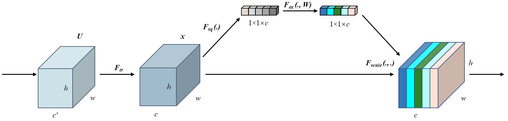
Figure 2 The attention mechanism of the traditional SENet.

$\begin{array}{ll}{F}_{sq}(x_c)=\frac{1}{h\times w}{\displaystyle \sum _{i=1}^h{\displaystyle \sum _{j=1}^w{x}_c(i,j),}}& (2)\end{array}$

$\begin{array}{ll}Sigmoid(x_c\text{'})=\frac{1}{1+e^{-x_c\text{'}}},& (3)\end{array}$

where $x_c$ represents the cth element in the squeeze operation to generate channel statistics through GAP, while h and w denote the height and width of the feature map, and $x_c\text{'}$ indicate the feature channel after undergoing the squeeze and excitation operations.

However, SENet for channel attention suffers from complexity, and fully connected layers resulting in excessive computational load. In addition, marine data often contain noise and redundant information, impacting the inversion of mesoscale eddy temperature structure. Not all information from each channel data is usable, leading to adopt an adaptive thresholding strategy for each channel. This approach has been widely employed in the signal and image recognition fields (Zhao et al., 2020), and shrinks input data towards zero. Figure 3 illustrates the structural diagram of the residual multi-channel attention module proposed in this paper. The threshold generated by the sigmoid function is not only positive but also appropriately scaled, ensuring normal gradient iteration. Below are the computational method and derivative of adaptive thresholding in Equations 4 and 5:

$\begin{array}{ll}y=soft(x,\tau )=\{\begin{array}{l}x-\tau ,x>\tau ,\\ 0,\left|x\right|\le \tau ,\\ x+\tau ,x<-\tau .\end{array},& (4)\end{array}$

$\begin{array}{ll}\frac{{\partial }_y}{{\partial }_x}=\{\begin{array}{l}1,x>\tau ,\\ 0,\left|x\right|\le \tau ,\\ 1,x<-\tau .\end{array},& (5)\end{array}$

Figure 3

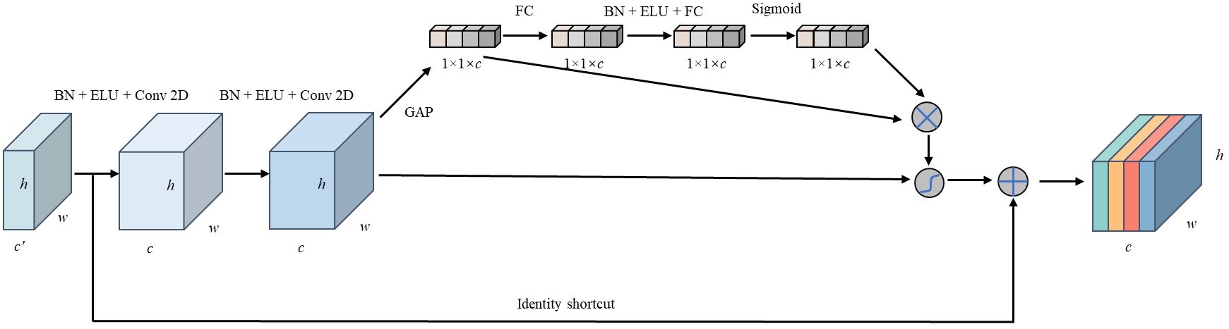
Figure 3 The structure of the residual multi-channel attention module with the adaptive threshold.

where the features of the input and output are respectively denoted by x and y, and the adaptive threshold τ is determined based on the pre-extracted feature map.

The attention mechanism module can be integrated with an end-to-end training method and various deep neural networks. In this paper, we implement the fusion of mixed attention and multi-channel attention with the residual module of the network. Due to the smaller input data, the convolution kernel size of 2 × 2 with a stride of 1 is applied to extract spatial and multi-channel features. Edge padding is used to fill the missing areas of the matrix, and the size of the output feature map generated is the same as the input feature map. The residual channel attention module consists of two main steps: the first step involves processing the input feature map through the residual connection, while the second step is to obtain multi-channel adaptive weights. Firstly, the input feature map through two convolution layers to extract features. Next, the multi-channel channel weights are determined using the adaptive threshold method based on two fully connected layers with the sigmoid activation function and multiplied by the GAP matrix to obtain channel weights. Batch Normalization (BN) is a commonly employed feature normalization strategy in various deep-learning models to reduce the internal covariate shift.

3.1.3 ELU activation function

The exponential linear unit (ELU) activation function has the same positive axis as the rectified linear unit (ReLU) activation function but introduces soft saturation for the negative axis instead of zero output (Kim et al., 2020). Equations (6, 7) provide the mathematical expressions for the ELU function and its derivative. ELU offers the same advantages as ReLU for the positive axis, but it also defines the negative axis, resulting in an overall output close to zero. In comparison to LeakyReLU, which also activates the negative axis, ELU has a soft saturation region with a decaying slope, providing certain robustness to models. Additionally, the parameter α controls the slope change of the function, with gradients closer to natural gradients, further accelerating the learning process.

$\begin{array}{ll}ELU(x)=\{\begin{array}{l}x,x\ge 0\\ \alpha (e^x-1),\text{x}<0\end{array}& (6)\end{array}$

$\begin{array}{ll}\frac{dELU}{dx}=\{\begin{array}{c}1, \\ \alpha e^x,\end{array}\begin{array}{c} x\ge 0\\ x<0\end{array},& (7)\end{array}$

where x represents input features, while α is a hyperparameter that is adjusted in the same way as other hyperparameters, typically set to 1.

Figure 4 illustrates the comprehensive architecture of ERCACN, which is a variant of the residual network and includes residual multi-channel attention modules (RCAM), canonical processing modules (BN), active modules (ELU), GAP and FC. Initially, the input data undergoes the convolution layer with 10 filters of the size 2 × 2, followed by the BN and activation function layer, resulting in a 5 × 5 × 10 feature map. The feature map is subsequently processed sequentially through three blocks of residual multi-channel attention modules with the adaptive threshold. By using both channel and spatial attention mechanisms, it concentrates on the “what” (channels) and “where” (spatial) aspects of the input data, which optimizes the feature extraction by dynamically adjusting the contribution of each channel according to its relative significance. Consequently, the feature map dimensions change to 16, 24 and 32. The extracted high-dimensional features are processed by a final fully connected layer with 800 neurons, leading to the prediction of ESTA. The Mean Square Error (MSE) loss function is selected for training due to its smooth, continuous curve, making it conducive to rapid convergence with gradient descent algorithms. The Equation 8 is as follows:

$\begin{array}{ll}\text{MSE}=\frac{{\displaystyle {\sum }_{i=1}^n{(Y_{obs,i}-Y_{pre,i})}^2}}{n}& (8)\end{array}$

Figure 4

Figure 4 The structure of ERCACN.

where $Y_{obs,i}$ indicates the temperature anomaly observed by Argo, and $Y_{pre,i}$ represents the temperature anomaly predicted by the model at the corresponding location. Table 2 presents the hyperparameters and the optimal value determined through experimental trials conducted during the model training process. In order to prevent overfitting, the ERCACN model incorporates several techniques, including L2 regularization, dropout, and early stopping. The tanh function is applied for initial low-dimensional feature extraction, while the ELU function is used as the activation function for subsequent layers. Adaptive Moment Estimation (Adam) is chosen as the optimizer for model training, enabling automatic adjustment of the learning rate without being impacted by gradient scaling transformations (Liu et al., 2023; Pasta et al., 2023).

Table 2

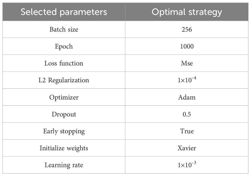
Table 2 Hyperparameter settings during the model training.

Figure 5 illustrates the comprehensive process of estimating ESTA utilizing the ERCACN model. Firstly, the temperature profiles of mesoscale eddies are extracted by combining the mesoscale eddy trajectory dataset from 2001 to 2017 with Argo profile data. Next, ESTA from Argo observations is generated by subtracting the temperature background field from WOA18 as the label data for the ERCACN model. The SLA and SSTA data are closely linked to the temperature structure of the water column caused by mesoscale eddies and wind stress can impact the mesoscale eddy motion and mixing processes (Wang et al., 2023; Yao et al., 2023). Therefore, multiple scales and variables of satellite remote sensing data, including SLA, SSTA, SSWSA, UWA and VWA, are selected based on the location information of mesoscale eddies and Argo profiles, and applied as the input of training and testing datasets for the ERCACN model. The datasets of mesoscale eddies, Argo and satellite data are matched in both temporal and spatial aspects. The data from 2001 to 2015 are classified into 13,161 anticyclonic eddies and 13,971 cyclonic eddies based on the properties of mesoscale eddies as training datasets. Since mesoscale eddies typically have a range of hundreds of kilometers and the satellite data has a spatial resolution of 0.25°, approximately five pixels matching mesoscale eddies, the 5 × 5 satellite data matrix centered around Argo profiles is meticulously chosen, containing abundant spatial information features. In the training dataset, diverse satellite variable data are individually subjected to data processing and normalization procedures. The resulting input data are subsequently arranged into the 5 × 5 × 5 matrix, which contains multivariate satellite data obtained from both the observation points and their surrounding areas.

Figure 5

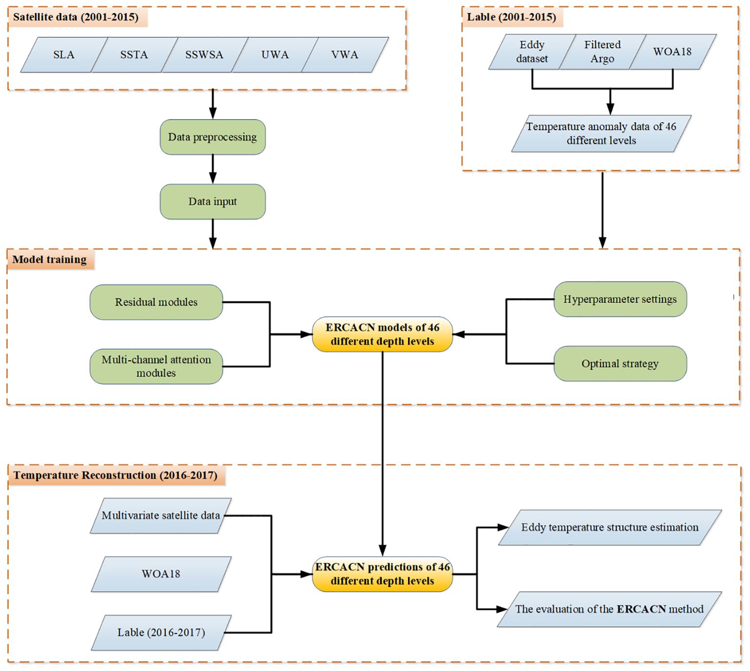
Figure 5 The overall flowchart of estimating ESTA based on ERCACN models.

Next, the ERCACN models are trained on the training set to acquire appropriate weights for ESTA estimations. Multivariate satellite remote sensing data and observed temperature anomaly data are used as the input and target output, respectively. Based on the different levels of WOA18 data, models are divided into 46 levels spanning depths from 5 m to 1000 m. Eventually, distinct models are individually trained for the anticyclonic and cyclonic mesoscale eddies, leading to the generation of 92 models.

Multivariate surface data at the locations of eddies with Argo profiles from 2016 to 2017, consisting of 2772 anticyclonic mesoscale eddy and 2706 cyclonic mesoscale eddy samples, are inputted into the 92 trained ERCACN models to estimate temperature anomalies at corresponding depths during model testing. The predictions are combined with WOA18 background temperature data to derive inversion results for the mesoscale eddy structures. Subsequently, the temperature values at the 0m level of SST data are utilized to fill the temperature structures, producing temperature structures for both anticyclonic and cyclonic mesoscale eddies from 0 to 1000 m.

3.2 Compared models

Various machine learning and deep learning methods commonly used in ocean temperature estimation are compared with the proposed the ERCACN model to evaluate its effectiveness. Among them, machine learning models such as MLR and RFR, have been previously employed in ocean temperature estimation (Guinehut et al., 2012; Su et al., 2018; Jeong et al., 2019). In addition, significant progress has been achieved in deep learning methodologies like the CNN architecture in this field (Su et al., 2021; Yu et al., 2021). These models are selected for comparison in estimating ESTA, with parameters and variables adjusted accordingly.

MLR: Based on ordinary least squares, this algorithm fits a linear model to predict the relationship between the dependent variable and multiple independent variables. Since the MLR model assumes a linear relationship, its effectiveness is usually limited when dealing with multivariate nonlinear relationships.

RFR: It is an ensemble learning algorithm based on decision trees, which constructs multiple decision trees and combines them into a powerful regression model for estimating ESTA. It has the capability to capture nonlinear relationships between different variables. However, the model structure is relatively simple, and it may encounter performance bottlenecks when dealing with high-order features in complex nonlinear data relationships.

CNNs: The sequential CNN model is designed, including CNN, batch normalization, the ELU activation function and fully connected layers. Through a data pipeline, the output of the previous layer serves as the input to the next layer. To validate the performance, the identical convolutional layer parameters and fully connected layer parameters are selected for comparison with the ERCACN model, along with the same parameter settings and loss functions. Finally, the extracted high-dimensional features are also inputted into a fully connected layer with 800 nodes to predict ESTA.

4 Results and discussion

In this section, the ESTA values estimated by the ERCACN model are compared and evaluated with Argo profiles including anticyclonic and cyclonic eddies in the observation region. Furthermore, the estimation performances of other methods using different combinations of sea surface features are compared under the same regional and training dataset conditions. In addition, the selected test dataset spans from 2016 to 2017.

To effectively evaluate the performance of various models, commonly used evaluation metrics were selected to analyze the accuracy of results in estimating ESTA.

(1) The Root Mean Square Error (RMSE), an important statistical metric utilized across various domains including meteorology, geographic information systems and machine learning, serves as a crucial tool for assessing the accuracy of the models. It quantifies the disparity between actual observed values. $Y_{obs,i}$ and model predictions $Y_{pre,i}$, enabling the evaluation of predictive capability and accuracy. The Equation 9 is as follows:

$\begin{array}{ll}\text{RMSE}=\sqrt{\frac{{\displaystyle {\sum }_{i=1}^n{(Y_{obs,i}-Y_{pre,i})}^2}}{n}}.& (9)\end{array}$

(2) The correlation coefficient (R), a statistical metric, is employed to measure the relationship between two variables. It evaluates the strength and direction of the association between $Y_{obs,i}$ and $Y_{pre,i}$, which holds significant importance in data analysis and decision. The Equation 10 is presented below:

$\begin{array}{ll}\text{R}=\frac{{\displaystyle {\sum }_{i=1}^n(Y_{obs,i}-\overline{Y_{obs,i}})(Y_{pre,i}-\overline{Y_{pre,i}})}}{\sqrt{{\displaystyle {\sum }_{i=1}^n{(Y_{obs,i}-\overline{Y_{obs,i}})}^2}}\sqrt{{\displaystyle {\sum }_{i=1}^n{(Y_{pre,i}-\overline{Y_{pre,i}})}^2}}}.& (10)\end{array}$

(3) Error indicates that the RMSE of temperature anomalies estimated by models at each depth layer occupies the ratio of the average temperature measured by Argos. The Equation 11 is as follows:

$\begin{array}{ll}\text{Error}=\frac{1}{\overline{Y_{pre,i}}}\sqrt{\frac{{\displaystyle {\sum }_{i=1}^n{(Y_{obs,i}-Y_{pre,i})}^2}}{n}}\times 100\%.& (11)\end{array}$

4.1 Comparison of different methods

4.1.1 Feature combinations and evaluations

Table 3A summarizes the performance of the anticyclonic estimations on the test dataset from 2016 to 2017 for all methods. Consistent conclusions are found for all other methods. With the gradual increase in the number of surface variables in the training model, there is a corresponding enhancement in the optimization of the regression model performance. In Case 1, utilizing only the SLA data for training the ERCACN model without additional parameters, the overall RMSE on the test set is 0.8571°C and the R value is 0.7507. Among them, Case 4, incorporating all training variables included in the model training process, demonstrates the best performance with an RMSE value of 0.8328°C and an R value of 0.7758. The comparison of Cases 1 to 4 indicates that these surface values play a positive role in the ESTA prediction of the anticyclonic eddy during the estimation process. Furthermore, despite utilizing the ERCACN method with different variable combinations, the RMSE and R values consistently remain below 0.8767°C and above 0.7342, providing the stability and robustness of our proposed method.

Table 3

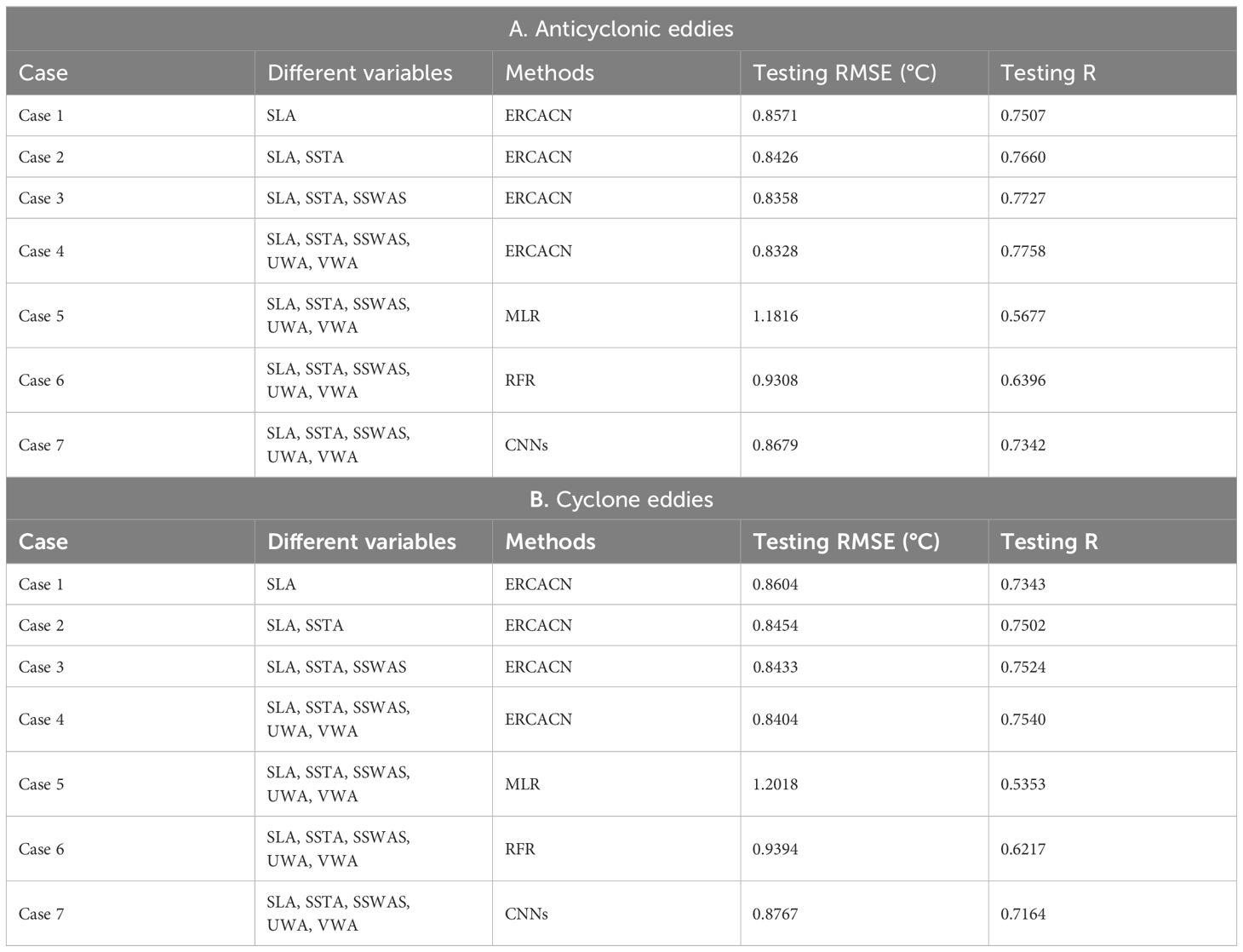
Table 3 Performance of ESTA vertical profiles fitted on the test data.

Similarly, compared to the linear Case 5 MLR, Case 4 exhibits remarkably better performance, which can be attributed to the method utilized to capture the nonlinear relationship between inputs and outputs. While MLR can fit the smooth characteristics of large-scale ocean temperature anomalies, the inherently nonlinear dynamics of mesoscale eddies impede the application of linear regressors such as MLR, leading to incapable of effectively capturing the nonlinear characteristics (Chelton et al., 2011b). In addition, compared to the RFR method applied in Case 6 (Su et al., 2018) and the CNNs method used in Case 7 (Yu et al., 2021), the performance of Cases 1 to 5 demonstrates lower RMSE and higher R values. As mentioned above, our approach, which employs the foundational architecture of convolutional neural networks, shares some similarities with the method used in Case 7. However, the key difference lies in the residual multi-channel attention module with the adaptive threshold in our proposed ERCACN model, enabling adaptive weight adjustments by considering the mutual interdependence between different features. Therefore, it shows that ERCACN outperforms other methods.

Table 3B presents the outcomes of the cyclonic eddy estimation under various parameters and methods, indicating similar performances with anticyclonic eddies. In Case 4, the RMSE is 0.8404°C, and the R value is 0.7540, which are the best results among all Cases. This highlights the superiority of our proposed ERCACN method over other approaches, whether applied to cyclonic or anticyclonic eddies. In addition, despite Case 1 only utilizing SLA as training input, it achieves an RMSE of 0.8604°C and an R value of 0.7343. In Case 5, although multivariable parameters are employed as input data, the utilization of MLR makes it challenging to capture the nonlinear information of mesoscale eddies, resulting in an RMSE of 1.2018°C and an R value of 0.5353. This significantly lower performance of Case 5 compared to other methods indirectly confirms the dominance of nonlinear characteristics in mesoscale eddies. Furthermore, Case 1, where only SLA parameters are used as input to train the ERCACN model, outperforms the RFR method in Case 6 and the CNNs method in Case 7, both of which utilize multiple parameters. These show the better performance of our proposed ERCACN model’s residual multi-channel attention module with the adaptive threshold.

Figure 6 illustrates the RMSE and R values of ESTA estimated for anticyclonic (A and C) and cyclonic (B and D) eddies. These are derived by using the combination of various surface features (SLA, SSTA, SSWAS, UWA and VWA) with MLR, RFR, CNNs and ERCACN methods on the test dataset at depths of 46 levels, corresponding to Cases 5, 6, 7 and 4 in Table 3. It can be observed that the vertical distribution of R and RMSE values obtained by various methods on the test dataset exhibits a similar pattern in terms of vertical structure. In Figure 6A, the RMSE values of diverse methods on the test dataset for anticyclonic eddies are depicted, highlighting the better performance of our proposed ERCACN model across all methods. Most RMSE values are below 1°C at most levels, demonstrating the superiority of our proposed method. Additionally, even near the surface, most RMSE values are within an acceptable range of below 1.2°C. CNNs also show a commendable performance, with a relatively smooth overall trend. Despite the reasonable performance of the RFR method, it exhibits fluctuations across different levels, indicating potential instability. MLR performs the worst among all methods, with a noticeable gap compared to other methods, primarily due to the dominance of nonlinear features of mesoscale eddies. Subsequently, Figure 6B illustrates the RMSE values of different methods for cyclonic eddies on the test dataset. Similarly, our proposed ERCACN model consistently exhibits the best performance and the RMSE values are below 1.2°C overall. The CNNs model achieves the second-best performance, followed by the RFR method with satisfactory results, while the MLR method exhibits the poorest performance. Additionally, regardless of anticyclonic or cyclonic eddies, our proposed ERCACN model achieves the best performance. For all cases, RMSE values above 200 m are relatively large, with a noticeable “bump” phenomenon observed in the depth range of 50 to 200 m, which may be associated with the depth of the mixed layer and the thermocline (de Boyer Montégut et al., 2004). The typical mixed layer depth in the Northwestern Pacific Ocean ranges from 50–100 m and remains relatively stable, leading to low RMSE values. In contrast, the water temperature in the thermocline experiences significant variations, while mesoscale eddies induce vertical and horizontal displacements of water masses, disrupting the vertical stratification of the temperature and promoting mixing between the oceanic mixed layer and the underlying thermocline. Consequently, this mixing process alters the thermal structure of the water column, leading to significant temperature fluctuations in the affected region, which complicates the estimation of ESTA values.

Figure 6

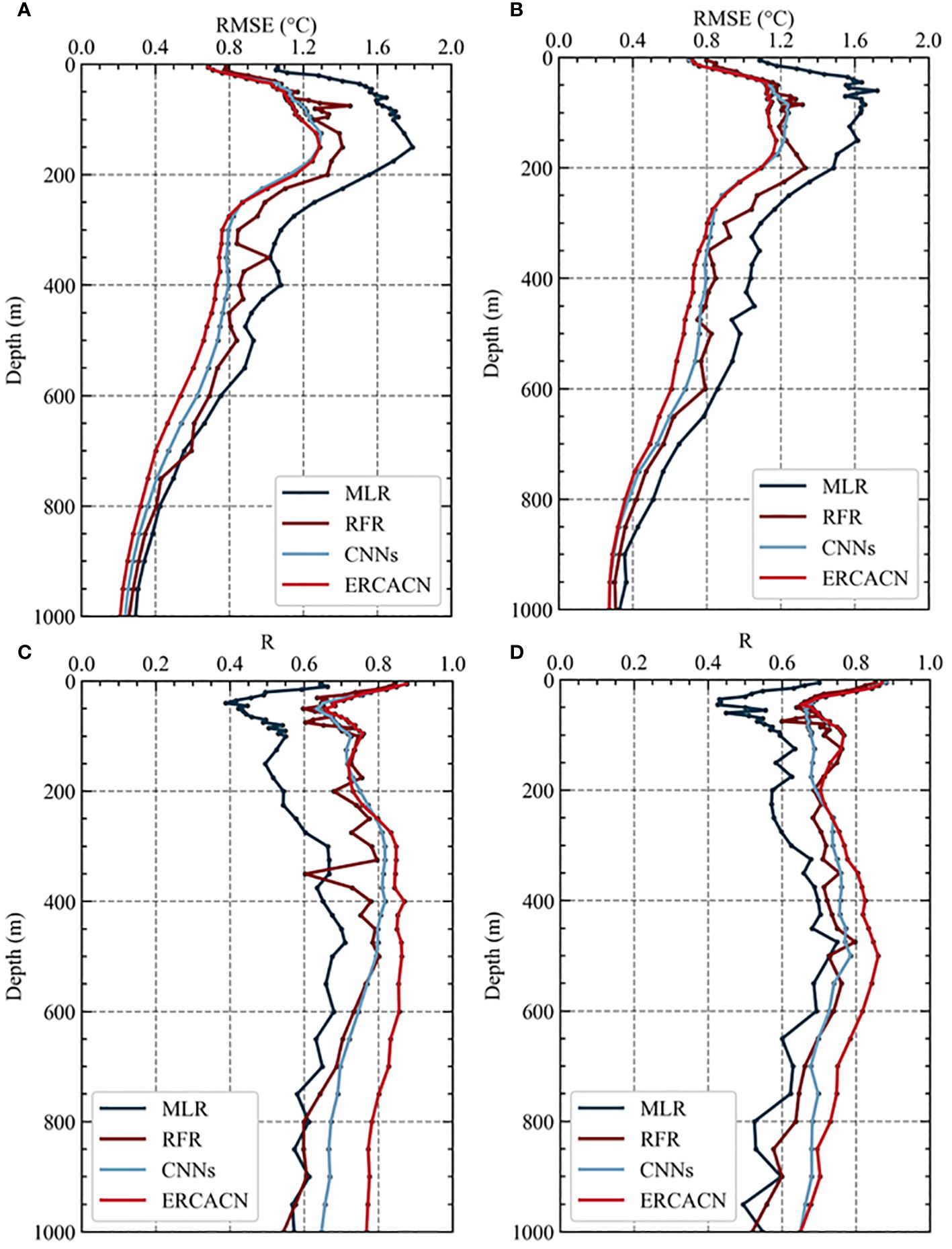
Figure 6 RMSE (°C) and R of ESTA which are estimated from different models by using all variable combinations for anticyclonic eddies (A, C) and cyclonic eddies (B, D) at depths of 5–1000 meters (comprising a total of 46 levels) on the test dataset. The distinct colors correspond to different methods, including MLR, RFR, CNNs and ERCACN.

Figure 6C presents the R values of ESTA estimates from 5–1000 m on the anticyclonic eddy test dataset obtained by applying different methods. These results indicate the correlation between the predicted values of various methods and the actual observed values. Overall, our proposed ERCACN model exhibits better performance compared to the CNNs model which shares a similar architecture but lacks our designed residual multi-channel attention module with the adaptive threshold, including most R values exceeding 0.7, particularly at deeper levels compared to other methods. This may be attributed to our designed residual multi-channel attention module with the adaptive threshold, which can capture the nonlinear features of anticyclonic eddies even under deep-sea conditions, leading to improved fitting results. Similar to the performance based on RMSE values, the CNNs method ranks second, the RFR method holds the third position and the MLR method performs the worst. Likewise, for cyclonic eddies, the performance rankings of these methods are similar in Figure 6D, with our proposed ERCACN model maintaining its superiority. Therefore, whether considering RMSE values or R values, our proposed ERCACN model can effectively extract features of mesoscale eddies from various remote sensing data to achieve the accurate estimation of ESTA from 5–1000 m.

4.1.2 Profile analysis

Figure 7 illustrates the comparison between the temperature profiles of eddies at depths ranging from 5 to 1000m obtained by various methods, including MLR, RFR, CNNs, ERCACN and the observed temperature from Argo profiles. Estimated temperature results for eddies can be derived by summing the temperature anomalies estimated by different models with the WOA18 temperature corresponding to the current location and time. Profiles of anticyclonic and cyclonic eddies are randomly selected based on the season and location. It is evident that the temperature profiles estimated by different methods closely resemble the observed profiles from Argo floats, indicating the feasibility of estimating subsurface temperature structures of eddies from satellite-derived sea surface data. Figure 7A specifically displays the estimated temperature profiles of anticyclonic eddies at different locations and seasons. The performance of MLR in estimating profiles is comparatively poor, with significant deviations from Argo profiles at some depths. While RFR performs relatively better than MLR, it still falls short compared to the results obtained by using deep learning methods such as CNNs and proposed ERCACN. Consequently, the temperature profiles of anticyclonic eddies estimated by deep learning methods exhibit greater proximity to the measured profiles. The CNNs method closely approximates the observed temperature profiles from Argo floats but shows slight deviations at certain depths. In addition, our proposed ERCACN method demonstrates a closer alignment with the measured temperature profiles, attributed to the design of our residual multi-channel attention module with the adaptive threshold, which assigns different weights to sea surface information channels and suppress noise signals to obtain accurate estimations of subsurface temperature profiles of anticyclonic mesoscale eddies.

Figure 7

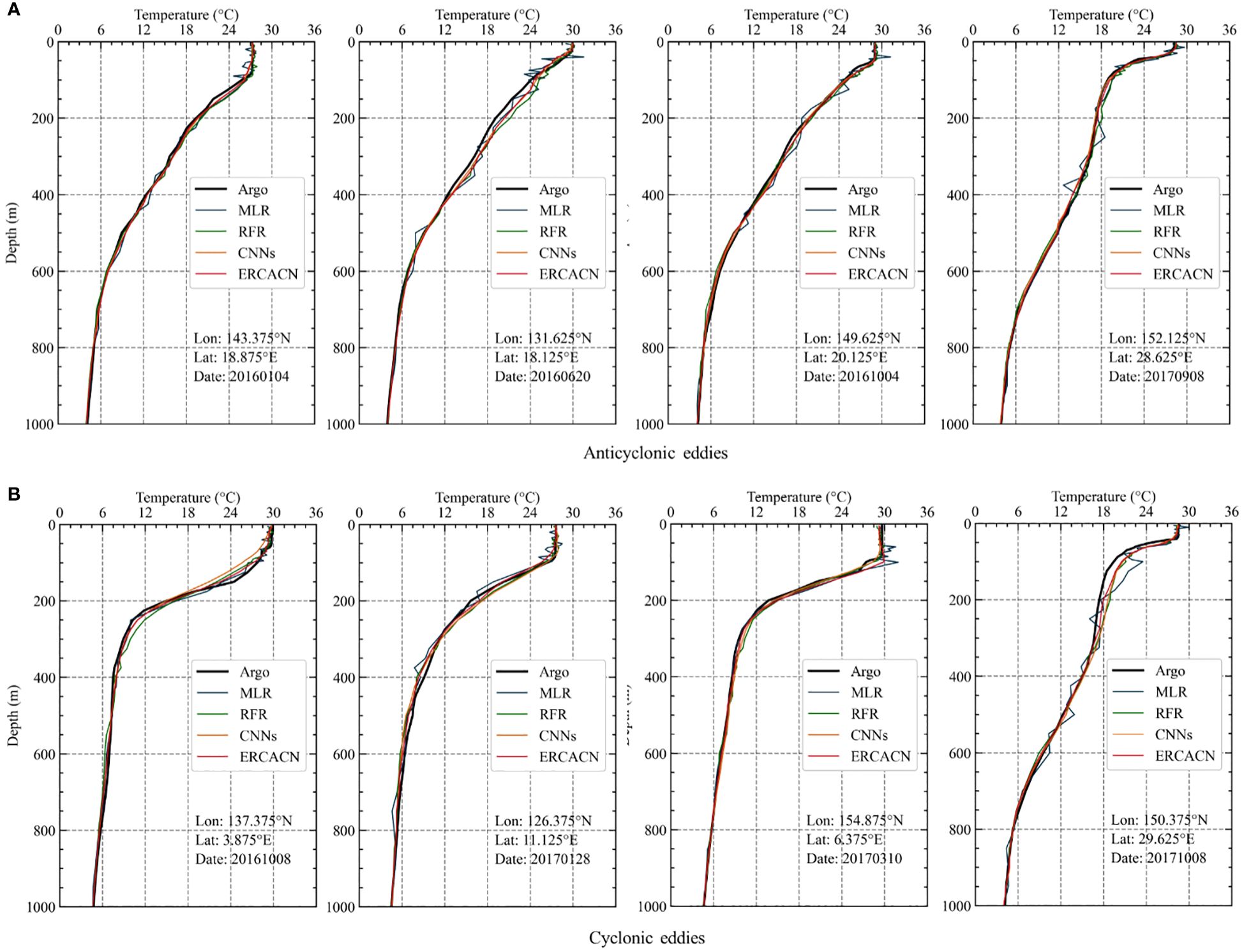
Figure 7 Different methods, including MLR, RFR, CNNs and ERCACN, are compared in terms of their estimation of eddy temperature profiles at depths ranging from 5 to 1000 meters with the temperature profiles obtained from Argo floats: (A) anticyclonic eddies, and (B) cyclonic eddies. The selection of profiles is made at random, considering the season and location.

Similarly, Figure 7B presents the estimated temperature profiles of cyclonic eddies across various locations and seasons. It is clear from the figure that different methods can estimate the temperature profiles of cyclonic eddies within acceptable ranges, demonstrating the correlation between various satellite-derived sea surface data and temperature structures at different depths. Similar to the results of anticyclonic eddies, the MLR method exhibits the poorest estimation performance, while the RFR method is comparable to the CNNs method, and the ERCACN method shows the best performance. Therefore, whether for anticyclonic or cyclonic eddies, nonlinear characteristics play a dominant role, which is the primary reason for the inferior performance of MLR. Conversely, our proposed ERCACN method consistently outperforms other methods in estimating temperature profiles across different mesoscale eddies with diverse locations and seasons, demonstrating the superiority and robustness of the ERCACN method, which can be applied to various regions in the Northwestern Pacific Ocean.

4.2 Result evaluations

4.2.1 The distribution of estimations for anticyclonic eddies

Figure 8 presents the accuracy distribution of temperature estimations for anticyclonic eddies using the ERCACN model and Argo observations. The temperature unit for the plotted points is °C, and the depths range are respectively (A) 40 m, (B) 85 m, (C) 125 m, (D) 200 m, (E) 400 m and (F) 700 m. The x-axis represents the temperature values of anticyclonic eddies measured by Argo at the current depth, while the y-axis displays the temperature values of anticyclonic eddies estimated by the ERCACN model at the current depth. RMSE and R values are also provided in figures for different depths. The y=x line is plotted to indicate that points closer to this line represent more accurate temperatures estimated by the ERCACN model. Additionally, due to the abundance of observational points in each layer, a Gaussian kernel is applied to perform kernel density estimation for the points in each layer, which is a non-parametric method for estimating the probability density function of a random variable (Viver et al., 2024). Points are shaded red to indicate higher concentration areas. In Figure 8, most red points in all subplots are concentrated around or near the y=x line, suggesting closer agreement between temperature estimations of anticyclonic eddies by the ERCACN model and Argo observations at different depths, demonstrating the accuracy and robustness of our proposed ERCACN model. Furthermore, the deviations between the temperature estimations of anticyclonic eddies by the ERCACN model and the data obtained by Argos are within reasonable ranges across different depths.

Figure 8

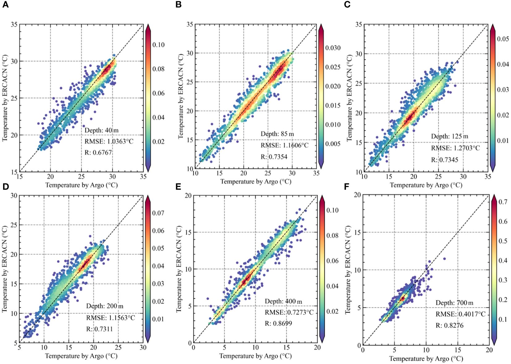
Figure 8 The accuracy analysis of the anticyclonic mesoscale eddy temperatures estimated by the ERCACN model and those observed by Argos at different depths. Depths of (A) 40m, (B) 85m, (C) 125m, (D) 200m, (E) 400m and (F) 700m.

Figure 8A depicts the distribution of temperatures for anticyclonic eddy at a depth of 40 m, with corresponding RMSE and R values of 1.0363°C and 0.6767. The data points cluster closely around or near the y=x line, with temperature estimations typically exceeding 23°C due to the shallow depth. Figure 8F exhibits the distribution of temperatures for anticyclonic eddy at a depth of 700 m, with corresponding RMSE and R values of 0.4017°C and 0.8276, and temperatures of most points cluster around 5°C. Figures 8B-E represent the temperature distributions of anticyclonic eddies at depths of 85 m, 125 m, 200 m and 400 m respectively. The clustering of temperature points for anticyclonic eddies gradually shifts downward with increasing depths. In addition, the proximity of temperature points to the y=x line across different depths demonstrates the accuracy and robustness of our proposed ERCACN model in this study. Furthermore, Figures 8A-C show the temperature estimations of anticyclonic eddies by the ERCACN model in the mixed and thermocline layers. Despite encountering the broad spectrum of temperatures, the temperature points largely converge with the y=x line, underscoring the model’s effectiveness in accurately estimating ESTA even in deep levels with complex thermal structures such as the mixed and thermocline layers.

4.2.2 The distribution of estimations for cyclonic eddies

Similar to the temperature estimations for anticyclonic mesoscale eddies, Figure 9 shows the accuracy distribution of temperature estimations for cyclonic eddies predicted by the ERCACN model compared to Argo observations. The selected depths for visualization remain consistent at (A) 40 m, (B) 85 m, (C) 125 m, (D) 200 m, (E) 400 m and (F) 700 m, enabling direct comparisons with temperature estimations for anticyclonic mesoscale eddies at corresponding depths. Additionally, the precision of temperature estimations by the ERCACN model at different depths exhibits a similar pattern to that of anticyclonic eddies, indicating a depth-dependent influence on accuracy. Furthermore, the distribution of temperature estimations for cyclonic mesoscale eddies at different depths falls within the reasonable margin of error.

Figure 9

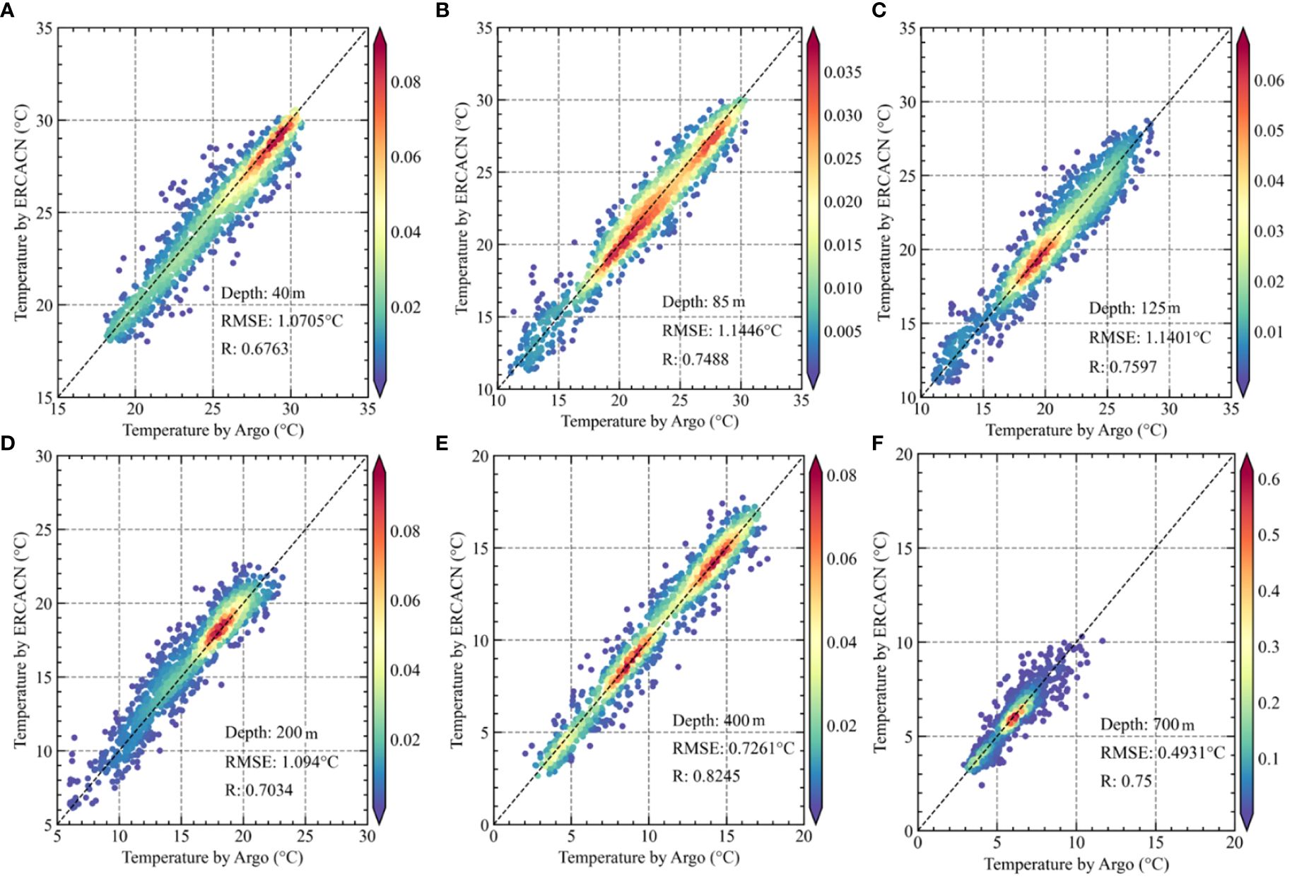
Figure 9 The accuracy analysis of the cyclonic mesoscale eddy temperatures estimated by the ERCACN model and those observed by Argos at different depths. Depths of (A) 40m, (B) 85m, (C) 125m, (D) 200m, (E) 400m and (F) 700m.

In Figure 9A, the ERCACN model predicts the temperature distribution of cyclonic eddies at a depth of 40 m, generating RMSE and R values of 1.0705°C and 0.6763 respectively, which align with the values obtained for anticyclonic mesoscale eddies. In addition, there is a noticeable trend of reduced temperature clustering compared to the results for anticyclonic eddies. Figure 9B shows the temperature distribution of cyclonic eddies at a depth of 85 m, presenting RMSE and R values of 1.1446°C and 0.7488 respectively. Most points cluster around 20°C, indicating a lower temperature relative to the temperature observations for anticyclonic eddies. This disparity could be attributed to cyclonic eddies displacing colder deep-ocean water towards the surface, thus replacing the original water and causing a decline in temperature. Figure 9C depicts the temperature distribution of cyclonic eddies at a depth of 125 m, exhibiting a similar pattern. As the depth increases, most points in Figures 9D-F converge near the y=x line, confirming the capability of the ERCACN model to accurately estimate cyclonic eddy temperatures at various depths. Moreover, although the occurrence of outliers may slightly affect the overall precision of the estimations of the ERCACN model, their frequency remains within acceptable limits, as depicted in Figure 9. In summary, the temperature estimates derived from the ERCACN model for both anticyclonic and cyclonic eddies at various depths closely correspond to temperature observations from Argo profiles, which could validate the accuracy and robustness of our proposed ERCACN model.

4.2.3 Error evaluation

Figure 10 illustrates that RMSE values occupy the percentage of the mean temperature observed by Argo for estimating ESTA at different depths, denoting the error through the MLR, RFR, CNNs and ERCACN methods. Figure 10A shows the error performance of various models concerning anticyclonic eddies. The error exhibits an increasing trend with depth, followed by a subsequent decrease. Initially, the MLR method demonstrates the worst performance, with errors exceeding 10% at most depths. It indicates linear methods have inadequate predictive capabilities for forecasting temperature results for anticyclonic mesoscale eddies, which are characterized by significant nonlinear features. Subsequently, the performance of the RFR method fluctuates considerably at different depths, with the majority of errors remaining below 10%, representing a significant improvement compared to the MLR method. Moreover, the CNNs method shows additional enhancement compared to the RFR method, closely approaching our proposed ERCACN method at shallower depths. However, as depth increases, the ERCACN method achieves smaller prediction errors, with most errors falling below 8% at various depths. In addition, the error peaks around 200m, possibly due to spatial variations induced by anticyclonic eddies at the thermocline, which may influence the ability of the ERCACN model to estimate ESTA.

Figure 10

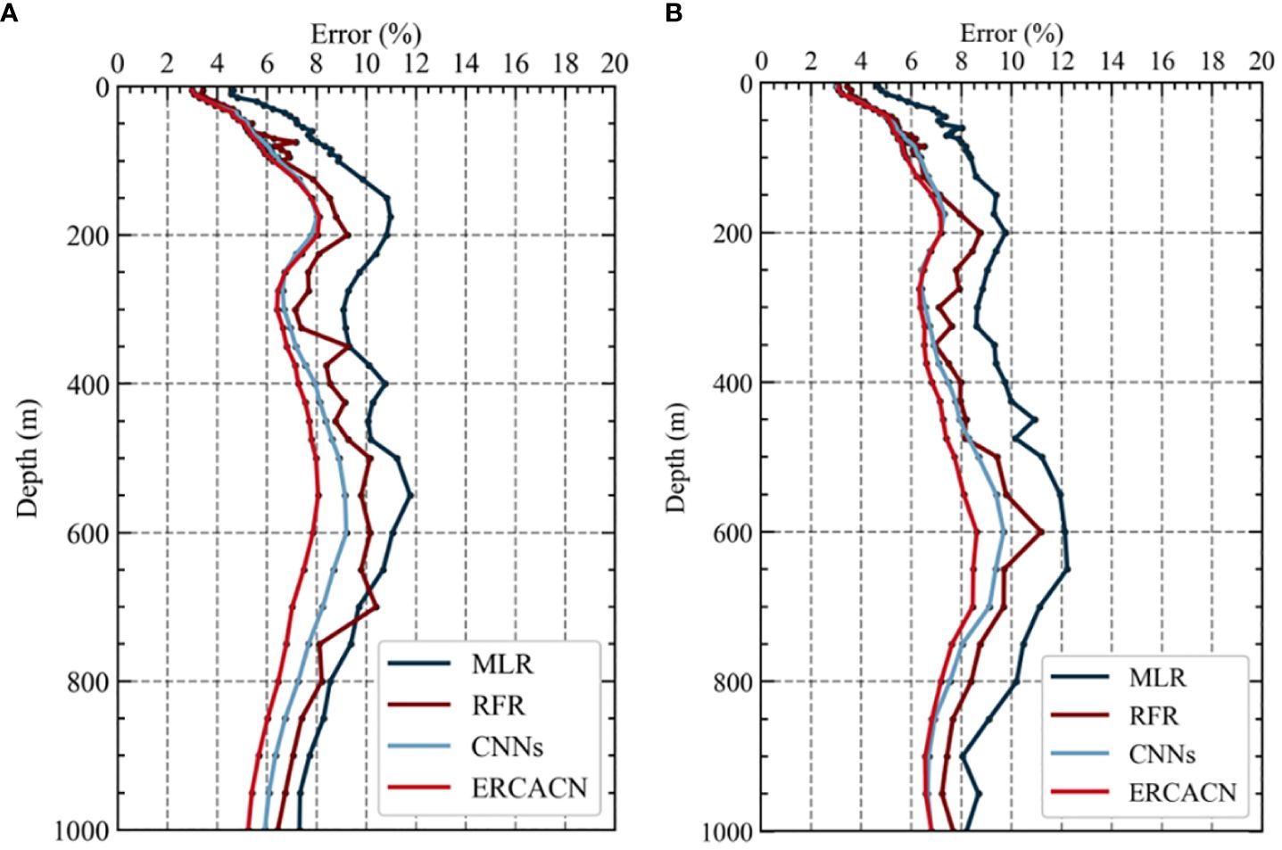
Figure 10 The Error values in estimating ESTA at various depths across different models, including (A) anticyclonic eddies and (B) cyclonic eddies.

Figure 10B shows the error of various models concerning cyclonic mesoscale eddies, exhibiting a trend of initial increase followed by a subsequent decline at deeper levels. However, unlike anticyclonic eddies, the errors for cyclonic eddies peak around 600 m due to the vertical impact, which typically extends to the deeper depths. Cyclonic mesoscale eddies induce the upward movement of deeper water masses, thereby affecting deeper layers. In contrast, anticyclonic eddies generally influence shallower depths, resulting in the downward movement of warm surface water masses. Similarly, the MLR method consistently exhibits the worst performance in error analysis, with values mostly below 12%. Errors for the RFR method largely remain below 10%, which closely compares to the result produced by the CNNs method. The ERCACN method demonstrates the optimal performance, with errors usually below 8% at different depths, which are within acceptable thresholds.

In summary, the ERCACN method demonstrates the accuracy and robustness in temperature estimations for both anticyclonic and cyclonic mesoscale eddies at various depths, highlighting its effectiveness in predicting mesoscale eddy temperatures using surface remote sensing information. Moreover, the ERCACN method exhibits superior performance including 46 different layers at various depths, meeting the requirements for high-precision resolution in estimating ESTA. Furthermore, the inherent limitations of MLR and RFR models necessitate the transformation of two-dimensional sea surface features into a one-dimensional format. This process restricts the utilization of spatial information, thereby hindering their performance compared to deep learning methods. Notably, the better performance exhibited by RFR relative to MLR indicates the importance of using algorithms capable of effectively handling complex nonlinear relationships between input features and target variables, particularly when estimating ESTA. In comparison to the CNNs model, our proposed ERCACN model demonstrates more remarkable performance. Unlike traditional CNN which processes all features uniformly, the ERCACN model incorporates an attention mechanism, enabling the network to prioritize the most influential features, thereby enhancing the identification of key features. Moreover, the integration of a residual CNN with the attention mechanism facilitates the dynamic adjustment of attention weights across different regions, effectively capturing long-range dependencies and optimizing model performance. An adaptive thresholding strategy is implemented to mitigate the impact of noise interference and redundant features in order to enhance the robustness and accuracy of the model.

4.3 Metrics analysis of the monthly results

Figure 11 illustrates the temporal variations in estimating the RMSE and R values for the temperature anomaly of anticyclonic eddies using the test dataset at depths of 50 m, 100 m, 150 m and 300 m by the ERCACN model. The results at various depths fall within an acceptable range. The RMSE value peaked at a depth of 100 m in October 2016, while the R value hit its nadir at 50m depth in November 2017. RMSE values generally increase during autumn at different depths, while corresponding R values decrease. This trend may be attributed to the decreased frequency of anticyclonic eddies during autumn, along with the limited profiles collected by Argos, thereby affecting the capability of the ERCACN model to estimate ESTA. In addition, compared to other depth levels, the RMSE value is generally lower at 300 m depth, with a correspondingly higher R value, indicating a relatively consistent capability of the ERCACN model to estimate ESTA on a time scale. This observation may be associated with the generally lower temperature at 300 m depth compared to other depths. The RMSE and R values at depths of 50 m, 100 m, and 150 m display consistent temporal variations, potentially owing to the subsidence of surface seawater induced by anticyclonic mesoscale eddies affecting shallower depths, deviating from the pattern at 300 m depth. Furthermore, the RMSE and R values at depths of 100 m and 150 m remain consistently similar throughout the observation period, due to their location at the thermocline layer within analogous oceanic structure.

Figure 11

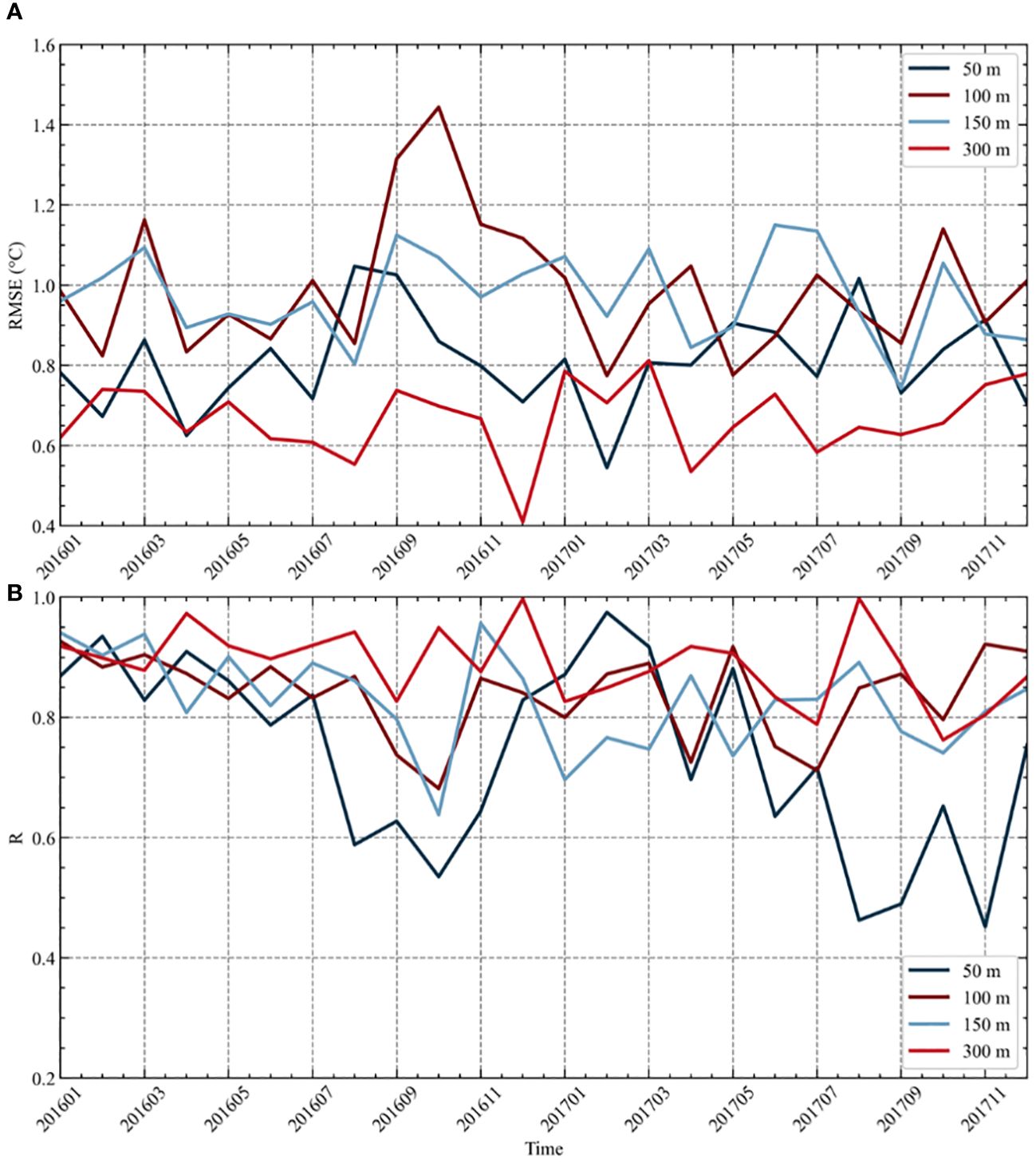
Figure 11 The (A) RMSE and (B) R values of anticyclonic eddies at depths of 50m, 100m, 150m and 300m obtained from the ERCACN model across various time points on the testing dataset spanning from 2016 to 2017.

Similarly, The ERCACN model depicts the temporal changes in predicting the RMSE and R values for eddy temperature anomalies of cyclonic mesoscale at depths of 50 m, 100 m, 150 m, and 300 m in Figure 12. It is evident that the results at different depths fall within a reasonable range. The RMSE value for the estimated temperature of cyclonic eddies peaked at a depth of 100 m in October 2016, while the R value reached its minimum at a depth of 50 m in May 2017. Analogous to anticyclonic eddies, RMSE values during autumn show a general upward trend across various depths, while the corresponding R values exhibit a downward trend. The overall trends of RMSE values at depths of 50 m, 100 m, 150 m and 300 m, as well as corresponding R values, are similar, indicating the consistent capability of the ERCACN model to estimate the temperature anomaly of cyclonic eddies at these depth levels. This phenomenon may be attributed to the upward movement of deeper seawater induced by cyclonic eddies, affecting deeper depths and resulting in similar trends of seawater across these depth levels. Significant variations in R values across different depth levels over time suggest discrepancies in the ERCACN model’s estimation of cyclonic eddy temperature anomalies in different months, which deserves further exploration in future studies.

Figure 12

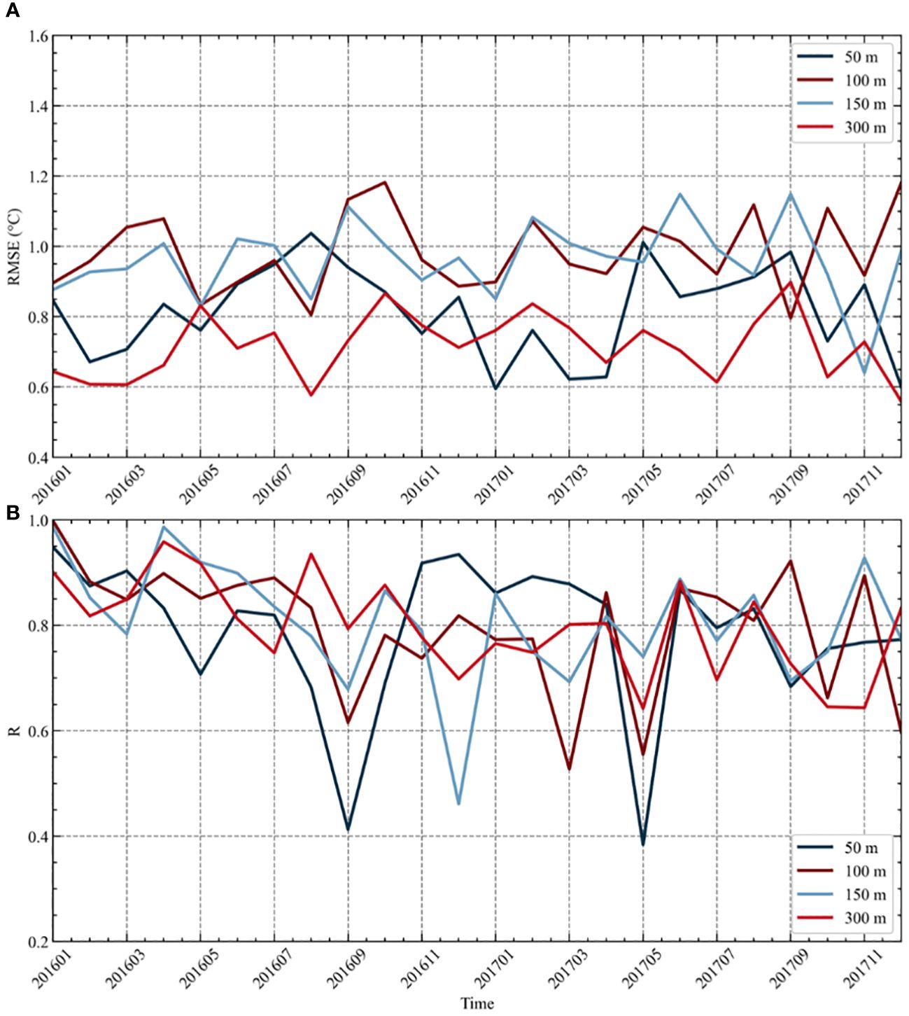
Figure 12 The (A) RMSE and (B) R values of cyclonic eddies at depths of 50m, 100m, 150m and 300m obtained from the ERCACN model across various time points on the testing dataset spanning from 2016 to 2017.

To quantify discrepancies in estimating ESTA at various depths and in different months by using the ERCACN model, this study applied the Error as a judgment threshold. The evaluation threshold of 8% was adopted to assess accuracy monthly at different depths. In the shallow ocean, the ERCACN model’s estimations of error range for temperature anomalies are generally consistent across all months. However, in deeper waters, the error in ESTA slightly exceeds the threshold. This discrepancy may arise from the decrease in average temperature observed by Argos with increasing depth, resulting in a higher percentage of RMSE in the observed temperature average. Among the ERCACN model’s estimation, 87.71% meet the accuracy threshold for anticyclonic mesoscale eddies, and the percentage is 88.45% for cyclonic mesoscale eddies. Overall, the ERCACN model’s estimation of ESTA on the test data achieves an 88.08% compliance rate with the 8% error as a threshold.

5 Conclusions

The Northwestern Pacific Ocean, owing to its distinctive regional oceanic features, is recognized as one of the global hotspots for mesoscale eddies. In this study, the combination of diverse surface remote sensing data including SLA, SST, SSWSA, UWA and VWA is designed and the ERCACN model is proposed, which successfully estimates ESTA at depths ranging up to 1000 m across 46 levels in the Northwestern Pacific Ocean. The model makes up for the lack of the observed temperature data of mesoscale eddies, providing data with a temporal resolution of one day and a spatial resolution of 0.25°. Through validation using independent Argo profiles, the ERCACN model demonstrates more accurate estimations of three-dimensional structures of ESTA compared to other methods. In summary, the results indicate an 88.08% conformity rate with the 8% error threshold, affirming the effectiveness and robustness of this combination approach and the proposed ERCACN model for temperature field estimations.

However, there is a systematic bias in the temporal and spatial alignment between Argo data and mesoscale eddies. With the continuous deployment of Argo profiles, the phenomenon could be further improved. In addition, the gridded data from satellite remote sensing observations leads to spatial resolution loss and interpolation errors, hindering accurate estimations of the three-dimensional temperature structure of mesoscale eddies. Furthermore, the spatial resolution of input satellite images at different levels may impact the accuracy and precision of the model, and future plans involve exploring and evaluating its influence on predictive performance and computational efficiency. Finally, the estimation of ESTA represents only the initial step in applying deep learning methods to obtain subsurface oceanic variables from surface information. Future research will focus on deriving salinity fields, velocity fields, and other variables of mesoscale eddies while concurrently enhancing temperature estimation precision.

Data availability statement

The original contributions presented in the study are included in the article/supplementary material. Further inquiries can be directed to the corresponding authors.

Author contributions

SL: Conceptualization, Data curation, Formal analysis, Investigation, Methodology, Software, Visualization, Writing – original draft, Writing – review & editing. AZ: Writing – review & editing, Funding acquisition, Project administration, Supervision. HZ: Writing – review & editing, Data curation, Formal analysis, Investigation, Validation. JL: Project administration, Writing – review & editing, Funding acquisition, Supervision. YL: Writing – review & editing, Funding acquisition, Resources.

Funding

The author(s) declare financial support was received for the research, authorship, and/or publication of this article. This study is supported by National Key R&D Program Project of China (2023YFB3907202).

Acknowledgments

We thank all authors, reviewers, and editors that have contributed to this research topic.

Conflict of interest

Author AZ was employed by the company Blue Sea Intelligent Equipment Services Company Limited.

The remaining authors declare that the research was conducted in the absence of any commercial or financial relationships that could be construed as a potential conflict of interest.

Publisher’s note

All claims expressed in this article are solely those of the authors and do not necessarily represent those of their affiliated organizations, or those of the publisher, the editors and the reviewers. Any product that may be evaluated in this article, or claim that may be made by its manufacturer, is not guaranteed or endorsed by the publisher.

References

Ali M. M., Swain D., Weller R. A. (2004). Estimation of ocean subsurface thermal structure from surface parameters: A neural network approach. Geophys. Res. Lett. 31, 1–4. doi: 10.1029/2004GL021192

CrossRef Full Text | Google Scholar

An L., Liu X., Xu F., Fan X., Wang P., Yin W., et al. (2024). Different responses of plankton community to mesoscale eddies in the western equatorial Pacific Ocean. Deep Sea Res. Part I 203, 104219–104231. doi: 10.1016/j.dsr.2023.104219

CrossRef Full Text | Google Scholar

Bibby T. S., Gorbunov M. Y., Wyman K. W., Falkowski P. G. (2008). Photosynthetic community responses to upwelling in mesoscale eddies in the subtropical North Atlantic and Pacific Oceans. Deep Sea Res. Part II 55, 1310–1320. doi: 10.1016/j.dsr2.2008.01.014

CrossRef Full Text | Google Scholar

Capet A., Mason E., Rossi V., Troupin C., Faugère Y., Pujol I., et al. (2014). Implications of refined altimetry on estimates of mesoscale activity and eddy-driven offshore transport in the Eastern Boundary Upwelling Systems. Geophys. Res. Lett. 41, 7602–7610. doi: 10.1002/2014GL061770

CrossRef Full Text | Google Scholar

Chelton D. B., Gaube P., Schlax M. G., Early J. J., Samelson R. M. (2011a). The influence of nonlinear mesoscale eddies on near-surface oceanic chlorophyll. Science 334, 328–332. doi: 10.1126/science.1208897

PubMed Abstract | CrossRef Full Text | Google Scholar

Chelton D. B., Schlax M. G., Samelson R. M. (2011b). Global observations of nonlinear mesoscale eddies. Prog. Oceanogr. 91, 167–216. doi: 10.1016/j.pocean.2011.01.002

CrossRef Full Text | Google Scholar

Chen C., Liu Z., Li Y., Yang K. (2023a). Reconstructing subsurface temperature profiles with sea surface data worldwide through deep evidential regression methods. Deep Sea Res. Part I 197, 104054. doi: 10.1016/j.dsr.2023.104054

CrossRef Full Text | Google Scholar

Chen G., Chen X., Cao C. (2023b). Eddy trains and eddy jets tracked by constellated altimetry. Remote Sens. Environ. 296, 113746–113760. doi: 10.1016/j.rse.2023.113746

CrossRef Full Text | Google Scholar

Chen L., Dong C., Wang G. (2023c). The satellite-observed linkages between large-scale climate fluctuations and mesoscale eddy movements in the North Pacific. Geophys. Res. Lett. 50, e2023GL102820. doi: 10.1029/2023GL102820

CrossRef Full Text | Google Scholar

Chen Q., Cai C., Chen Y., Zhou X., Zhang D., Peng Y. (2024). TemproNet: A transformer-based deep learning model for seawater temperature prediction. Ocean Eng. 293, 116651–116664. doi: 10.1016/j.oceaneng.2023.116651

CrossRef Full Text | Google Scholar

Chen Z., Wang X., Liu L., Wang X. (2023d). Estimating three-dimensional structures of eddy in the south Indian ocean from the satellite observations based on the is QG method. Earth Space Sci. 10, e2023EA002991. doi: 10.1029/2023EA002991

CrossRef Full Text | Google Scholar

de Boyer Montégut C., Madec G., Fischer A. S., Lazar A., Iudicone D. (2004). Mixed layer depth over the global ocean: An examination of profile data and a profile-based climatology. J. Geophys. Res. Oceans 109. doi: 10.1029/2004JC002378

CrossRef Full Text | Google Scholar

Dobashi R., Ueno H., Matsudera N., Fujita I., Fujiki T., Honda M. C., et al. (2022). Impact of mesoscale eddies on particulate organic carbon flux in the western subarctic North Pacific. J. Oceanogr. 78, 1–14. doi: 10.1007/s10872-021-00620-7

CrossRef Full Text | Google Scholar

Dong D., Brandt P., Chang P., Schütte F., Yang X., Yan J., et al. (2017). Mesoscale eddies in the northwestern Pacific Ocean: three-dimensional eddy structures and heat/salt transports. J. Geophys. Res. Oceans 122, 9795–9813. doi: 10.1002/2017JC013303

CrossRef Full Text | Google Scholar

Dong C., Liu L., Nencioli F., Bethel B. J., Liu Y., Xu G., et al. (2022). The near-global ocean mesoscale eddy atmospheric-oceanic-biological interaction observational dataset. Sci. Data 9, 1–13. doi: 10.1038/s41597-022-01550-9

PubMed Abstract | CrossRef Full Text | Google Scholar

Dong C., McWilliams J. C., Liu Y., Chen D. (2014). Global heat and salt transports by eddy movement. Nat. Commun. 5, 1–6. doi: 10.1038/ncomms4294

CrossRef Full Text | Google Scholar

Guinehut S., Dhomps A.-L., Larnicol G., Le Traon P.-Y. (2012). High resolution 3-D temperature and salinity fields derived from in situ and satellite observations. Ocean Sci. 8, 845–857. doi: 10.5194/os-8-845-2012

CrossRef Full Text | Google Scholar

He Y., Feng M., Xie J., He Q., Liu J., Xu J., et al. (2021). Revisit the vertical structure of the eddies and eddy-induced transport in the leeuwin current system. J. Geophys. Res. Oceans 126, e2020JC016556. doi: 10.1029/2020JC016556

CrossRef Full Text | Google Scholar

Huang B., Liu C., Banzon V., Freeman E., Graham G., Hankins B., et al. (2021). Improvements of the daily optimum interpolation sea surface temperature (DOISST) version 2.1. J. Climate 34, 2923–2939. doi: 10.1175/JCLI-D-20-0166.1

CrossRef Full Text | Google Scholar

Huo J., Zhang J., Yang J., Li C., Liu G., Cui W. (2024). High kinetic energy mesoscale eddy identification based on multi-task learning and multi-source data. Int. J. Appl. Earth Obs. Geoinf. 128, 103714–103722. doi: 10.1016/j.jag.2024.103714

CrossRef Full Text | Google Scholar

Jeong Y., Hwang J., Park J., Jang C. J., Jo Y.-H. (2019). Reconstructed 3-D ocean temperature derived from remotely sensed sea surface measurements for mixed layer depth analysis. Remote Sens. 11, 3018–3036. doi: 10.3390/rs11243018

CrossRef Full Text | Google Scholar

Kim D., Kim J., Kim J. (2020). Elastic exponential linear units for convolutional neural networks. Neurocomputing 406, 253–266. doi: 10.1016/j.neucom.2020.03.051

CrossRef Full Text | Google Scholar

Li X., Wang Q., Danilov S., Koldunov N., Liu C., Müller V., et al. (2024). Eddy activity in the Arctic Ocean projected to surge in a warming world. Nat. Clim. Change 14, 156–162. doi: 10.1038/s41558-023-01908-w

CrossRef Full Text | Google Scholar

Liu S., Fu X., Xu H., Zhang J., Zhang A., Zhou Q., et al. (2023). A fine-grained ship-radiated noise recognition system using deep hybrid neural networks with multi-scale features. Remote Sens. 15, 2068. doi: 10.3390/rs15082068

CrossRef Full Text | Google Scholar

Liu F., Tang S. (2018). Influence of the interaction between typhoons and oceanic mesoscale eddies on phytoplankton blooms. J. Geophys. Res. Oceans 123, 2785–2794. doi: 10.1029/2017JC013225

CrossRef Full Text | Google Scholar

Lu W., Su H., Yang X., Yan X.-H. (2019). Subsurface temperature estimation from remote sensing data using a clustering-neural network method. Remote Sens. Environ. 229, 213–222. doi: 10.1016/j.rse.2019.04.009

CrossRef Full Text | Google Scholar

Mahaur B., Mishra K. K., Singh N. (2023). Improved Residual Network based on norm-preservation for visual recognition. Neural Networks 157, 305–322. doi: 10.1016/j.neunet.2022.10.023

PubMed Abstract | CrossRef Full Text | Google Scholar

McGillicuddy D. J. (2016). Mechanisms of physical-biological-biogeochemical interaction at the oceanic mesoscale. Annu. Rev. Mar. Sci. 8, 125–159. doi: 10.1146/annurev-marine-010814-015606

CrossRef Full Text | Google Scholar

Mears C. A., Scott J., Wentz F. J., Ricciardulli L., Leidner S. M., Hoffman R., et al. (2019). A near-real-time version of the cross-calibrated multiplatform (CCMP) ocean surface wind velocity data set. J. Geophys. Res. Oceans 124, 6997–7010. doi: 10.1029/2019JC015367

CrossRef Full Text | Google Scholar

Nencioli F., Dall’Olmo G., Quartly G. D. (2018). Agulhas ring transport efficiency from combined satellite altimetry and argo profiles. J. Geophys. Res. Oceans 123, 5874–5888. doi: 10.1029/2018JC013909

CrossRef Full Text | Google Scholar

Pasta E., Carapellese F., Faedo N., Brandimarte P. (2023). Data-driven control of wave energy systems using random forests and deep neural networks. Appl. Ocean Res. 140, 103749–103763. doi: 10.1016/j.apor.2023.103749

CrossRef Full Text | Google Scholar

Ping B., Su F., Han X., Meng Y. (2021). Applications of deep learning-based super-resolution for sea surface temperature reconstruction. IEEE J. Sel. Topics Appl. Earth Observ. Remote Sens. 14, 887–896. doi: 10.1109/JSTARS.2020.3042242

CrossRef Full Text | Google Scholar

Pun I.-F., Lin I.-I., Ko D. S. (2014). New generation of satellite-derived ocean thermal structure for the western north pacific typhoon intensity forecasting. Prog. Oceanogr. 121, 109–124. doi: 10.1016/j.pocean.2013.10.004

CrossRef Full Text | Google Scholar

Purkiani K., Haeckel M., Haalboom S., Schmidt K., Urban P., Gazis I.-Z., et al. (2022). Impact of a long-lived anticyclonic mesoscale eddy on seawater anomalies in the northeastern tropical Pacific Ocean: a composite analysis from hydrographic measurements, sea level altimetry data, and reanalysis model products. Ocean Sci. 18, 1163–1181. doi: 10.5194/os-18-1163-2022

CrossRef Full Text | Google Scholar

Sammartino M., Buongiorno Nardelli B., Marullo S., Santoleri R. (2020). An artificial neural network to infer the Mediterranean 3D chlorophyll-a and temperature fields from remote sensing observations. Remote Sens. 12, 4123. doi: 10.3390/rs12244123

CrossRef Full Text | Google Scholar

Shan X., Jing Z., Gan B., Wu L., Chang P., Ma X., et al. (2020). Surface heat flux induced by mesoscale eddies cools the Kuroshio-Oyashio extension region. Geophys. Res. Lett. 47, e2019GL086050. doi: 10.1029/2019GL086050

CrossRef Full Text | Google Scholar

Shankar Manche S., Nayak R. K., Sikhakolli R., Bothale R. V., Chauhan P. (2024). Characteristics of mesoscale eddies and their evolution in the north Indian ocean. Prog. Oceanogr. 221, 103213. doi: 10.1016/j.pocean.2024.103213

CrossRef Full Text | Google Scholar

Shi Z., Guan C., Li Q., Liang J., Cao L., Zheng H., et al. (2022). Detecting marine organisms via joint attention-relation learning for marine video surveillance. IEEE J. Ocean. Eng. 47, 959–974. doi: 10.1109/JOE.2022.3162864

CrossRef Full Text | Google Scholar

Su H., Li W., Yan X.-H. (2018). Retrieving temperature anomaly in the global subsurface and deeper ocean from satellite observations. J. Geophys. Res. Oceans 123, 399–410. doi: 10.1002/2017JC013631

CrossRef Full Text | Google Scholar

Su H., Wang A., Zhang T., Qin T., Du X., Yan X.-H. (2021). Super-resolution of subsurface temperature field from remote sensing observations based on machine learning. Int. J. Appl. Earth Obs. Geoinf. 102, 102440–102450. doi: 10.1016/j.jag.2021.102440

CrossRef Full Text | Google Scholar

Su H., Wu X., Yan X.-H., Kidwell A. (2015). Estimation of subsurface temperature anomaly in the Indian Ocean during recent global surface warming hiatus from satellite measurements: A support vector machine approach. Remote Sens. Environ. 160, 63–71. doi: 10.1016/j.rse.2015.01.001

CrossRef Full Text | Google Scholar

Su H., Yang X., Lu W., Yan X.-H. (2019). Estimating subsurface thermohaline structure of the global ocean using surface remote sensing observations. Remote Sens. 11, 1598–1619. doi: 10.3390/rs11131598

CrossRef Full Text | Google Scholar

Sun W., An M., Liu J., Liu J., Yang J., Tan W., et al. (2022). Comparative analysis of four types of mesoscale eddies in the Kuroshio-Oyashio extension region. Front. Mar. Sci. 9. doi: 10.3389/fmars.2022.984244

PubMed Abstract | CrossRef Full Text | Google Scholar

Ueno H., Bracco A., Barth J. A., Budyansky M. V., Hasegawa D., Itoh S., et al. (2023). Review of oceanic mesoscale processes in the North Pacific: Physical and biogeochemical impacts. Prog. Oceanogr. 212, 102955. doi: 10.1016/j.pocean.2022.102955

CrossRef Full Text | Google Scholar

Viver T., Conrad R. E., Rodriguez-R L. M., Ramírez A. S., Venter S. N., Rocha-Cárdenas J., et al. (2024). Towards estimating the number of strains that make up a natural bacterial population. Nat. Commun. 15, 1–13. doi: 10.1038/s41467-023-44622-z

PubMed Abstract | CrossRef Full Text | Google Scholar

Wang C., Liu F. (2024). Influence of oceanic mesoscale eddies on the deep chlorophyll maxima. Sci. Total Environ. 917, 170510. doi: 10.1016/j.scitotenv.2024.170510

PubMed Abstract | CrossRef Full Text | Google Scholar

Wang H., Qiu B., Liu H., Zhang Z. (2023). Doubling of surface oceanic meridional heat transport by non-symmetry of mesoscale eddies. Nat. Commun. 14, 1–10. doi: 10.1038/s41467-023-41294-7

PubMed Abstract | CrossRef Full Text | Google Scholar

Wu X., Yan X.-H., Jo Y.-H., Liu W. T. (2012). Estimation of subsurface temperature anomaly in the North Atlantic using a self-organizing map neural network. J. Atmos. Oceanic Technol. 29, 1675–1688. doi: 10.1175/JTECH-D-12-00013.1

CrossRef Full Text | Google Scholar

Xie H., Xu Q., Cheng Y., Yin X., Jia Y. (2022). Reconstruction of subsurface temperature field in the South China sea from satellite observations based on an attention U-net model. IEEE Trans. Geosci. Remote Sens. 60, 1–19. doi: 10.1109/TGRS.2022.3200545

CrossRef Full Text | Google Scholar

Xu L., Li P., Xie S.-P., Liu Q., Liu C., Gao W. (2016). Observing mesoscale eddy effects on mode-water subduction and transport in the North Pacific. Nat. Commun. 7, 1–9. doi: 10.1038/ncomms10505

CrossRef Full Text | Google Scholar

Yan H., Wang H., Zhang R., Chen J., Bao S., Wang G. (2020). A dynamical-statistical approach to retrieve the ocean interior structure from surface data: SQG-mEOF-R. J. Geophys. Res. Oceans 125, e2019JC015840. doi: 10.1029/2019JC015840

CrossRef Full Text | Google Scholar

Yang P., Jing Z., Wu L. (2018). An assessment of representation of oceanic mesoscale eddy-atmosphere interaction in the current generation of general circulation models and reanalyses. Geophys. Res. Lett. 45, 11,856–11,865. doi: 10.1029/2018GL080678

CrossRef Full Text | Google Scholar

Yang G., Wang F., Li Y., Lin P. (2013). Mesoscale eddies in the northwestern subtropical Pacific Ocean: Statistical characteristics and three-dimensional structures. J. Geophys. Res. Oceans 118, 1906–1925. doi: 10.1002/jgrc.20164

CrossRef Full Text | Google Scholar

Yang Y., Wang D., Wang Q., Zeng L., Xing T., He Y., et al. (2019). Eddy-induced transport of saline kuroshio water into the Northern South China sea. J. Geophys. Res. Oceans 124, 6673–6687. doi: 10.1029/2018JC014847

CrossRef Full Text | Google Scholar

Yao H., Ma C., Jing Z., Zhang Z. (2023). On the vertical structure of mesoscale eddies in the kuroshio-oyashio extension. Geophys. Res. Lett. 50, e2023GL105642. doi: 10.1029/2023GL105642

CrossRef Full Text | Google Scholar

Yu F., Wang Z., Liu S., Chen G. (2021). Inversion of the three-dimensional temperature structure of mesoscale eddies in the Northwest Pacific based on deep learning. Acta Oceanolog. Sin. 40, 176–186. doi: 10.1007/s13131-021-1841-z

CrossRef Full Text | Google Scholar

Yuan Q., Hu J. (2023). Spatiotemporal characteristics and volume transport of lagrangian eddies in the northwest pacific. Remote Sens. 15, 4355–4374. doi: 10.3390/rs15174355

CrossRef Full Text | Google Scholar

Zhang Y., Liu Z., Zhao Y., Wang W., Li J., Xu J. (2014a). Mesoscale eddies transport deep-sea sediments. Sci. Rep. 4, 1–7. doi: 10.1038/srep05937

CrossRef Full Text | Google Scholar

Zhang Z., Tian J., Qiu B., Zhao W., Chang P., Wu D., et al. (2016). Observed 3D structure, generation, and dissipation of oceanic mesoscale eddies in the South China sea. Sci. Rep. 6, 1–11. doi: 10.1038/srep24349

PubMed Abstract | CrossRef Full Text | Google Scholar

Zhang Z., Wang W., Qiu B. (2014b). Oceanic mass transport by mesoscale eddies. Science 345, 322–324. doi: 10.1126/science.1252418

PubMed Abstract | CrossRef Full Text | Google Scholar

Zhang Z., Zhang Y., Wang W., Huang R. X. (2013). Universal structure of mesoscale eddies in the ocean. Geophys. Res. Lett. 40, 3677–3681. doi: 10.1002/grl.50736

CrossRef Full Text | Google Scholar

Zhao N., Huang B., Yang J., Radenkovic M., Chen G. (2023). Oceanic eddy identification using pyramid split attention U-net with remote sensing imagery. IEEE Geosci. Remote Sens. Lett. 20, 1–5. doi: 10.1109/LGRS.2023.3243902

CrossRef Full Text | Google Scholar

Zhao D., Xu Y., Zhang X., Huang C. (2021). Global chlorophyll distribution induced by mesoscale eddies. Remote Sens. Environ. 254, 112245–112257. doi: 10.1016/j.rse.2020.112245

CrossRef Full Text | Google Scholar

Zhao Y., Zhang H., Gao Z., Guan W., Nie J., Liu A., et al. (2022). A temporal-aware relation and attention network for temporal action localization. IEEE Trans. Image Process 31, 4746–4760. doi: 10.1109/TIP.2022.3182866

PubMed Abstract | CrossRef Full Text | Google Scholar

Zhao M., Zhong S., Fu X., Tang B., Pecht M. (2020). Deep residual shrinkage networks for fault diagnosis. IEEE Trans. Ind. Inf. 16, 4681–4690. doi: 10.1109/TII.9424

CrossRef Full Text | Google Scholar