A high-precision interpretable framework for marine dissolved oxygen concentration inversion

Variations in Marine Dissolved Oxygen Concentrations (MDOC) play a critical role in the study of marine ecosystems and global climate evolution. Although artificial intelligence methods, represented by deep learning, can enhance the precision of MDOC inversion, the uninterpretability of the operational mechanism involved in the “black-box” often make the process difficult to interpret. To address this issue, this paper proposes a high-precision interpretable framework (CDRP) for intelligent MDOC inversion, including Causal Discovery, Drift Detection, RuleFit Model, and Post Hoc Analysis. The entire process of the proposed framework is fully interpretable: (i) The causal relationships between various elements are further clarified. (ii) During the phase of concept drift analysis, the potential factors contributing to changes in marine data are extracted. (iii) The operational rules of RuleFit ensure computational transparency. (iv) Post hoc analysis provides a quantitative interpretation from both global and local perspectives. Furthermore, we have derived quantitative conclusions about the impacts of various marine elements, and our analysis maintains consistency with conclusions in marine literature on MDOC. Meanwhile, CDRP also ensures the precision of MDOC inversion: (i) PCMCI causal discovery eliminates the interference of weakly associated elements. (ii) Concept drift detection takes more representative key frames. (iii) RuleFit achieves higher precision than other models. Experiments demonstrate that CDRP has reached the optimal level in single point buoy data inversion task. Overall, CDRP can enhance the interpretability of the intelligent MDOC inversion process while ensuring high precision.

1 Introduction

Marine Dissolved Oxygen Concentration (MDOC) serves as an essential indicator for evaluating seawater conditions and plays a significant role in the regulation of the global climate. The decrease in MDOC, also known as marine hypoxia, can significantly affect marine ecosystems, potentially leading to extensive marine biota mortality events (Karadurmus and Sari, 2022; Brock et al., 2023; Wang et al., 2023b). This phenomenon directly impacts 10% to 12% of the global population reliant on coastal ecosystems for sustenance (Breitburg et al., 2018; Li et al., 2023b). On the other hand, the production of nitrous oxide (N₂O) shows obvious sensitivity to variations in MDOC. Particularly in conditions of reduced MDOC, there is a notable rise in N₂O production (Suntharalingam et al., 2000; Jin and Gruber, 2003; Hutchins and Capone, 2022). Despite the importance of MDOC research within the field of marine science, the accessibility of MDOC data remains relatively constrained in comparison to data on temperature and salinity. This limitation hinders comprehensive research efforts in this area (Wang et al., 2020). Currently, widely used marine data include buoy measurements of MDOC and other marine elements from the World’s Oceans Real-time Network Plan (ARGO)¹, as well as the World Ocean Database (WOD)², which compiles datasets from various countries and organizations. However, initial deployments primarily focused on measuring temperature and salinity, meanwhile modern buoys face challenges related to calibration and drift (Johnson et al., 2017). Consequently, utilizing data such as temperature and salinity to infer MDOC holds great significance, making MDOC inversion highly meaningful.

The development of MDOC inversion methodologies has primarily undergone three stages: numerical computation, machine learning, and deep learning (Figure 1): Initially, numerical computation was employed for inversion calculations, but the associated computational costs were found to be excessively high; Nonetheless, the introduction of machine learning methodologies within the domain of artificial intelligence significantly reduced computational costs (Figure 1A); More recently, the deployment of deep learning models has further elevated computational precision, but the uninterpretable working mechanism of the “black-box” has led to the low interpretaiblity of these models (Figure 1B); After conducting research, we found that rule-based methods such as RuleFit, excelling in both precision and interpretability, have not been widely applied in oceanography, thus their adoption could effectively ensure high precision and inherent interpretability in marine intelligent inversion models (Figure 1C).

Figure 1

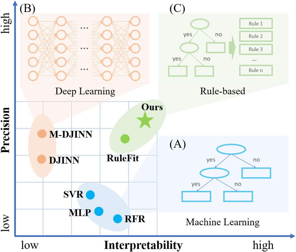
Figure 1 Precision and interpretability in MDOC inversion tasks. (A) Machine Learning; (B) Deep Learning; (C) Rule-based.

At present, there have been multiple approaches to address the MDOC inversion. Traditionally, using climate system models and low-order marine biogeochemical models for MDOC inversion has been a common practice (Matear and Hirst, 2003), while mathematical modeling is also a prevalent method for MDOC inversion (Naik and Manjappa, 2011). However, these traditional models have some limitations, such as slow computational speed, demanding equipment requirements, and high operational costs, making it difficult to implement streamlined inversion for MDOC.

Nowadays with the rapid expansion of marine datasets, machine learning has supassed traditional methods in robustness and has shown excellent performance in uncovering the complex nonlinear relationships between variables (Jiang et al., 2017), because of its faster computational speeds and lower dependence on data assumptions. And multiple machine learning algorithms have been emplyed to investigate the association between dissolved oxygen concentration and other elements. Ji et al. (2017) utilized eleven hydrochemical variables from the Wen-Rui Tang River to assess the accuracy of dissolved oxygen concentration inversion using Support Vector Regression (SVR). Giglio et al. (2018) attempted to use Random Forest Regression (RFR) to reproduce the dissolved oxygen concentration fields from the Southern Ocean State Estimate (SOSE), and explored the precision effects in specific boundary areas. Ross and Stock (2019) applied Multilayer Perceptron (MLP) to explore the relationship between monthly marine elements and dissolved oxygen concentration in Chesapeake Bay, analyzing stratification phenomena on a sub-seasonal scale. However, the structure of machine learning is relatively simple, leaving considerable room for the further boosting of the fitting precision.

Recently, deep learning has been employed to increase the precision of MDOC inversion based on single point buoy data. Wang et al. (2020) used DJINN and its improved version, M-DJINN, to clarify the relationship between dissolved oxygen concentration and other variables such as temperature and salinity, utilizing data from the World Ocean Database. Experimental evidence shows that the precision of deep learning networks significantly outperforms traditional machine learning algorithms. However, the interpretability of deep learning networks is limited by their hidden layers, which extensively abstract and transform input data nonlinearly, and involve large number of parameter. This complexity makes it difficult to understand how the model operates. As a result, current high-precision MDOC inversion methods encounter difficulties in gaining full trust from decision-makers in marine ecology, posing substantial risks in decision-making processes. Therefore, developing a fully interpretable, high-precision intelligent inversion framework for MDOC becomes a significant challenge to overcome.

Rule-based methodologies offer a practical solution for achieving interpretable computations with high precision. Friedman and Popescu (2008) introduced RuleFit, a model consisting of a linear combination of rules and linear components, where each rule is expressed through straightforward evaluative statements about the input variables’ values. This collection of rules can achieve predictive precision comparable to the best methods, with the added benefit of being easily interpretable. In recent years, RuleFit has seen widespread use in fields that emphasize the interpretability of artificial intelligence, such as intelligent healthcare. For instance, Carrazana-Escalona et al. (2022) used RuleFit to predict the characteristics of blood pressure parameters among 8 adolescent volunteers during dynamic pressure-bearing processes, and Luo et al. (2022) applied it to diagnose nasopharyngeal carcinoma in 1706 patients. These studies illustrate that RuleFit can provide operational rules for models with high precision, thus enhancing their inherent interpretability. Although rule-based methods have the advantages of high precision and interpretability, these methods still have certain limitations. Bénard et al. (2021) introduced SIRUS, which enhances the precision and stability of rule extraction by restricting decision tree node splits to empirical quantile positions. However, the conclusions provided by this method are too specific and verbose, making it difficult to analyze the rules. Additionally, Mollas et al. (2022) proposed LionForests, which is valued for its “conclusiveness”, demonstrating improved stability and interpretability. Nonetheless, this method still has shortcomings in terms of its coverage of the decision-making process. Zhang et al. (2023) introduced OptExplain, an algorithm that utilizes particle swarm optimization for the optimization process, but it is currently applicable only to classification tasks, which does not align with the MDOC inversion task. By contrast, RuleFit, with its broad application base and superior performance, excels in rule generation and offers ease of interpretation. Therefore, RuleFit is ultimately selected as the inversion model in this work.

In this paper, we introduce a framework that offers both high precision and interpretability for the intelligent inversion of MDOC. We have named this framework CDRP because it comprises Causal Discovery, Drift Detection, RuleFit Model, and Post Hoc Analysis. To clarify the causal relationships between marine elements, we adopt the PCMCI causal discovery method, which helps to remove weakly correlated relationships and elucidate the associations between MDOC and other relevant elements, thereby enhancing the effectiveness and interpretability of model learning. In addition, the concept drift detection technique is also used to further improve the precision of the intelligent model and to help users understand the key features of the data. This technique helps users select more representative data, known as key frame data, for training the intelligent inversion model. Additionally, to realize high-precision interpretable intelligent inversion at the computational aspect of the model, we utilize the rule-based RuleFit algorithm. This algorithm not only achieves high-precision inversion of MDOC but also aids in clarifying the internal mechanisms of intelligent computation by analyzing the extracted rules. Upon completion of training, we utilize post-hoc analysis techniques like SHAP and LIME to investigate the model’s operational mechanisms. Our focus is on obtaining quantitative insights into how different marine elements influence the climatological normals of MDOC, both in terms of magnitude and direction. The analysis shows that our framework CDRP produces results that align well with conclusions in marine literature. In summary, our contributions are mainly in the following five aspects: (i) We propose an interpretable artificial intelligence framework CDRP for achieving high-precision interpretability in the MDOC intelligent inversion process; (ii) The introduction of PCMCI enhances the interpretability of CDRP by elucidating the relationships between MDOC and other elements while eliminating the interference of weakly correlated elements; (iii) By utilizing concept drift detection, this paper ensures a more representative selection of training data and model tuning, thereby effectively elevating the model’s precision and interpretability based on data reduction; (iv) This study pioneers the application of the rule-based RuleFit model to marine ecology, enhancing both the inversion precision and the interpretability of the operational mechanism; (v) The validation of CDRP through causal discovery, rule analysis, SHAP, and LIME, and its consistency with conclusions in marine literature on MDOC, effectively ensures interpretability in the inversion process.

2 Materials and methods

2.1 Study area and dataset

After reviewing extensive literature and datasets, we have preliminarily identified several marine elements related to MDOC inversion, including temperature, salinity, pH, chlorophyll concentration, turbidity, CO₂ concentration, water column level, and sediment phosphorus. In further selection of these elements, we have considered the following aspects: Since both pH and CO₂ concentration are key indicators of ocean acidification, which creates redundancy in their impact mechanisms on MDOC, we have abandoned the CO₂ concentration in our study. Additionally, as the oceanographic data involved in the inversion task are two-dimensional, while water column level are inherently three-dimensional, we will not consider the water column level for MDOC inversion. Moreover, because turbidity already reflects certain changes in sediment phosphorus, and data on sediment phosphorus are difficult to obtain, we have decided to exclude the utilization of sediment phosphorus. Finally, we selected the following 5 marine elements for further exploration: temperature (OTMP), salinity (SAL), chlorophyll concentration (CLCON), turbidity (TURB), and pH.

The dataset used in this study was provided by the National Data Buoy Center (NDBC)³, which is part of the National Oceanic and Atmospheric Administration (NOAA). It includes data collected from about 100 moored buoys and Coastal-Marine Automated Network (C-MAN) stations. Additionally, it includes data from 55 Tropical Atmosphere Ocean (TAO) buoys that are deployed and maintained in the equatorial Pacific, covering a range from 9°N to 8°S and from 95°W to 165°E. This buoy network system automatically captures and transmits real-time meteorological and oceanographic data to the National Ocean Service (NOS), located in Maryland.

2.2 Description of the proposed framework

In this research, we introduce a high-precision interpretable framework aimed at resolving the MDOC inversion challenge. This framework (Figure 2) is principally segmented into four phases: Causal Discovery, Drift Detection, RuleFit Model, and Post Hoc Analysis. All interpretive actions are supported by validation from marine-related research literature, ensuring the professional integrity and logical consistency of the interpretive results. The details are outlined as follows:

Figure 2

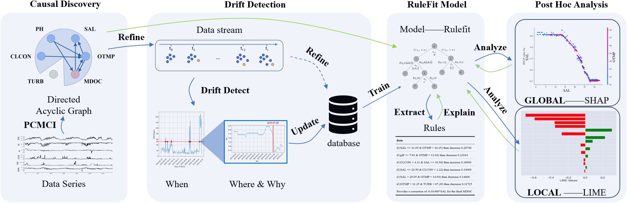
Figure 2 Framework of the proposed approach.

Causal Discovery: In this stage, we utilize the causal discovery algorithm PCMCI to learn the causal relationship among the marine elements. By removing elements with weakly correlated relationship, we eliminate the interference with the model learning process. Subsequently, we analyze the associations between MDOC and relevant elements, enhancing the overall interpretability of the framework.

Drift Detection: This phase involves calculating the drift degree in continuously batched stream data to identify the timing (When) and specific data distribution (Where) of concept drift occurrences. It also includes an analysis of the underlying reasons related to marine observation processes (Why). The data collected when concept drift occurs are marked as key frame data for the intelligent model’s training.

RuleFit Model: Training the RuleFit model with the dataset refined by key frame selection in the previous phase, elevates the precision of inversion and allows for the extraction of the model’s internal operational rules. Analyzing these rules offers a preliminary explanation of the model’s operational mechanism.

Post Hoc Analysis: Employing global-level SHAP analysis and local-level LIME analysis offers more detailed explanations of the RuleFit model’s operational mechanism. The insights derived from causal discovery, RuleFit’s rules, along with these analyses, demonstrate excellent consistency with conclusions in marine literature, thus greatly enhancing the interpretability of intelligent computations.

2.3 Causal discovery

To elucidate the causal relationships between each marine element and MDOC, we introduced the PCMCI algorithm for causal discovery. This method was proposed by Runge et al. (2019) and consists of two main stages:

(i) PC Algorithm: Used for causal relationship discovery in time series data. It iteratively employs independence testing to remove unrelated causal associations, converging to a small number of key causal relationships and constructing an initial causal relationship graph.

(ii) MCI Algorithm: Used for instantaneous conditional independence testing. It suppresses false positives for highly interdependent time series.

Given a dynamic system $X_t=\left\{X_t^1,\dots ,X_t^N\right\}$ of N representing marine elements considered at t time points, the following equation holds true (Equation 1):

$\begin{array}{ll}{X}_t^j=f_j(P(X_t^j),{\eta }_t^j)& (1)\end{array}$

where f_j represents some potential nonlinear functional dependencies, and $n_t^j$ denotes mutually independent dynamic noise $P(X_t^j)$ represents the causal parents of variable $X_t^j$ among all N elements in the past. This causal discovery method is based on the concept of conditional independence. By estimating the strength and direction of causal relationships between highly interdependent time series of multiple marine elements, it effectively removes the interference of weakly correlated marine elements in model learning. Furthermore, by classifying each marine element based on its association with MDOC, the interpretability of the overall framework can be effectively enhanced.

2.4 Drift detection

The dissolved oxygen station data utilized in this paper is presented as a continuous data stream. As time progresses, the distribution of input data may undergo significant changes, which may adversely affect the performance of the intelligent inversion model trained on historical data. This phenomenon is known as concept drift (Lu et al., 2018). Detecting concept drift enables adjustments to the intelligent inversion model to improve its precision. It also allows for explanations of changes in data distribution, linking these changes to variations in marine elements. The methodology employed in this paper utilizes incremental Gaussian Mixture Model (GMM) clustering for each data batch. This process calculates the drift degree between the current batch and historical marine data. It selects the most representative data exceeding a predefined threshold to compile a dataset, designated as key frame data, for training the inversion task (Yang et al., 2020). The formula for drift degree is defined as follows (Equation 2):

$\begin{array}{ll}{D}_t={\displaystyle \sum _i\frac{\left|X_t^i\right|}{\left|X_t\right|}d(X_t^i,{\widehat{X}}^i)}& (2)\end{array}$

In this context, |·| represents the number of marine data samples, and d(·) denotes the energy distance between marine data samples. X_t represents all the data of the current batch. $X_t^i$ and ${\widehat{X}}^i$ respectively represent the current batch data and the historical data for the i-th cluster. The formula for energy distance is defined as follows (Equation 3):

$\begin{array}{ll}d(X,Y)=(2A-B-C)/2A& (3)\end{array}$

Here, $A=\frac{1}{mn}{\displaystyle {\sum }_{i=1}^n{\displaystyle {\sum }_{j=1}^m\Vert x_i-y_i\Vert }}$ represents the average Euclidean distance between elements of marine features in two sets of marine data samples X and Y. $B=\frac{1}{n^2}{\displaystyle {\sum }_{i=1}^n{\displaystyle {\sum }_{j=1}^{\text{n}}\Vert x_i-x_j\Vert }}$ and $C=\frac{1}{m^2}{\displaystyle {\sum }_{i=1}^{\text{m}}{\displaystyle {\sum }_{j=1}^m\Vert y_i-y_j\Vert }}$ respectively represent the average Euclidean distance between elements within marine data samples X and Y.

2.5 Model computation

To elevate the computational precision and clarify the intrinsic operational mechanisms of the intelligent inversion model for MDOC, a rule-based ensemble method, RuleFit, has been adopted. This method constructs a model through a linear combination of rules and linear expressions, where each rule includes a concise set of statements about the individual input variables. Such collection of rules can achieve predictive precision comparable to that of the best methods. It also enables an initial understanding of the operational mechanism of the intelligent model through the analysis of principal rules (Friedman and Popescu, 2008). Specifically, given a marine data sample x = {x₁,x₂,…,x_n}^T ∈ Rⁿ, the RuleFit model is defined as follows (Wan et al., 2023) (Equation 4):

$\begin{array}{ll}{F}_{Rfit}(x)={\alpha }_0+{\displaystyle \sum _{k=1}^K{\alpha }_k{r}_k(x)+{\displaystyle \sum _{j=1}^n{\alpha }_j^{*}{l}_j(x_j)}}& (4)\end{array}$

Here, ${\alpha }_0\in R,{\alpha }_k\in R(k=0,1,\dots ,K),{\alpha }_j^{\ast }\in R(j=1,\dots ,n)$ represent the MDOC climatological normals, the coefficients for the rule terms of the intelligent inversion model, and the coefficients for the linear terms of intelligent inversion model, respectively. The rule terms are formed by combining judgment clauses for specific marine elements (r_k: Rⁿ → R), and the linear terms are comprised of functions related to specific marine elements (l_j: R → R).

2.6 Post hoc analysis

2.6.1 SHAP analysis

To provide a more comprehensive and reliable explanation of the operational mechanisms of the inversion model, we utilized SHAP (Shapley Additive Explanations) analysis. This approach quantitatively assesses the impact magnitude and direction that various marine elements have on the MDOC climatological normals from a global perspective. SHAP represents a game theory-based method for interpreting artificial intelligence models (Štrumbelj and Kononenko, 2014). It facilitates assessing the negative and positive effects that marine elements have on the output of the intelligent MDOC inversion model. Given an intelligent inversion model trained with marine data samples X_i = {x₁,x₂,…,x_n}^T, an explanation model (EM) is employed by SHAP to evaluate the contribution of each marine element to the intelligent inversion model. The details can be described in the following equation (Equations 5, 6):

$\begin{array}{ll}EM={\phi }_0+{\displaystyle \sum _{i=1}^n{\phi }_i{t}_i}& (5)\end{array}$

$\begin{array}{ll}{\phi }_i(f,x)={\displaystyle \sum _{t\subseteq x}\frac{\left|t\right|!(n-\left|t\right|-1)!}{n!}[f(t)-f(t\backslash i)]}& (6)\end{array}$

Where n is the number of marine elements, t_i is the simplification of marine element i, t_i ∈ R denotes the contribution of variable i to the artificial intelligence model, \ denotes the difference-set notation for set operations, and f indicates the interpretable artificial intelligence model.

2.6.2 LIME analysis

To better understand how intelligent inversion models work, especially at critical points like MDOC extrema, we intend to utilize the Local Interpretable Model-agnostic Explanations (LIME) analysis. This approach will allow us to examine how various marine elements influence the output of the intelligent inversion model. When a new observation is introduced, LIME creates an extended dataset consisting of perturbed samples and their corresponding model outputs. A linear explanatory model is then adjusted based on this dataset, applying weights according to the closeness of these sampled observations (Ribeiro et al., 2016). Through this approach, we can apply the interpretable model, which is tailored for local explanations (Chakraborty et al., 2021), to estimate the influence of marine elements on the MDOC extrema. Specifically, the definition of the local interpretable model g is as follows (Equation 7):

$\begin{array}{ll}g=\text{ arg min }L(f,g,{\pi }_x)+\Omega (\text{g})& (7)\end{array}$

Here, π_x measures how close the changed marine data instances are to each other, usually using a Gaussian kernel. L(f,g,π_x) shows how much the interpretable model g differs from the model f we want to explain, especially at MDOC extrema. Ω(g) measures the complexity of the interpretable model (such as the number of non-zero weights in a linear model).

2.7 Implementation and evaluation metrics

In this study, we applied the Python programming language, widely used in data science, along with key modules such as Numpy, scikit-learn, SHAP, and LIME. The configuration of our environment comprised Python 3.7, a 12th Gen Intel(R) Core(TM) i7–12700H, and Windows 11.

To evaluate the precision of CDRP within the MDOC inversion task, this study utilizes three widely recognized statistical and regression metrics to measure its performance: Mean Square Error (MSE), Accuracy (ACC), and Explained Variance Score (EVS).

Mean Squared Error (MSE) is defined as follows (Equation 8):

$\begin{array}{ll}MSE=\frac{1}{n}{\displaystyle \sum _{i=1}^n{({\widehat{y}}_i-y_i)}^2}& (8)\end{array}$

In this context, n denotes the total number of observations, with y_i indicating the observed value for the i-th observation, and ${\widehat{y}}_i$ representing the predicted value for it. A reduction in the MSE value signifies improved accuracy in the inversions. Consequently, the accuracy of the model is derived from the MSE as defined below (Equation 9):

$\begin{array}{ll}ACC=1-\frac{\frac{1}{n}{\displaystyle {\sum }_{i=1}^n{({\widehat{y}}_i-y_i)}^2}}{\frac{1}{n}{\displaystyle {\sum }_{i=1}^n{y}_i}}& (9)\end{array}$

Explained variance score (EVS) is defined as follows (Equation 10):

$\begin{array}{ll}EVS=1-\frac{Var(Y-\widehat{Y})}{Var(Y)}& (10)\end{array}$

Here, $\widehat{Y}$ denotes the predicted output, Y is the observed output in relation to $\widehat{Y}$, and Var represents variance. Importantly, the highest possible score is 1, with a lower score reflecting a decrease in the prediction’s adequacy, as shown by the variance in the dependent variables.

3 Result

3.1 Inversion performance

In this study, buoy data from various locations along the U.S. West Coast were employed, with the dataset for MDOC inversion comprising the first-hour average values of temperature (OTMP), salinity (SAL), chlorophyll concentration (CLCON), and pH (According to the causal discovery graph in Section 3.2.1, we excluded turbidity, which showed weak correlation with MDOC). SVR, RFR, MLP, DJINN, M-DJINN, and RuleFit were trained and evaluated utilizing this dataset. To validate the models’ performance in this study, data from January 1, 2016, to October 18, 2019, making up the initial continuous 80%, was designated as the training set. Conversely, data ranging from October 19, 2019, to February 22, 2022, representing the subsequent continuous 20%, was selected for the test set.

By continuously conducting concept drift detection on marine element data, organized in batches corresponding to one week’s duration, variations in drift degree are depicted in Figure 3. By setting an appropriate threshold, it becomes possible to accurately identify the dates when drifts occur. Following the identification of concept drift, data from those dates are merged with the dataset previously used for model training. The model is then retrained on this updated dataset. Upon setting the drift degree threshold at 12, eight specific instances of concept drift were detected. Figure 4 shows the distinct changes in data distribution for each instance of concept drift, highlighted by red lines. Based on comparisons of data before and after each detected instance of concept drift, preliminary analysis of the causative factors is presented as follows: The first concept drift occurred on March 12, 2016 (Figure 4A), where the pH decreased from 8.6 to 8.0. In contrast, on January 24, 2019 (Figure 4G), pH showed an increase. These changes may be attributed to the influence of upwelling and possible coastal discharge (Kroeker et al., 2020; Li et al., 2023a). On June 10, 2016 (Figure 4B), October 9, 2016 (Figure 4D), and March 28, 2019 (Figure 4H), there were significant increases in chlorophyll concentration, possibly due to the extensive proliferation of phytoplankton (Conley et al., 2007). Furthermore, fluctuations in temperature and salinity influenced by local coastal climate were effectively detected and corrected (Figures 4C, E, F).

Figure 3

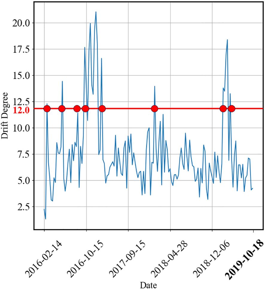
Figure 3 The variation of drift degree over time. (The red line represents the set drift threshold, and the red solid point is the dates when the concept drift detection is occurred).

Figure 4

Figure 4 (A–H) The data distribution at the date of concept drift. (The date when concept drift occurs is highlighted by a red line).

This research selected MDOC data samples from the first 30 days to pre train the inversion model, and then conducted concept drift detection in batches of 7 days. As shown in Figure 3, eight distinct instances of concept drift were detected. Together with 30 pre-trained data samples, the final key frame dataset comprised a total of 86 data samples, which shows a significant reduction compared to the overall 1080 MDOC training data samples. It is worth noting that the data reduction reduced the complexity and redundancy of training data, filtered out more informative features, and allowed the model to focus more on learning key features, effectively helping users improve their understanding of the overall features of the learning process (Atitey et al., 2024). Therefore, while improving the precision of MDOC inversion, it effectively enhanced the interpretability of the intelligent inversion process.

To assess the precision superiority of CDRP for MDOC inversion task, a comparative analysis was conducted between CDRP and several models currently used in this field, including SVR, RFR, MLP, DJINN, and M-DJINN. Despite the moderate novelty of the models compared in the experiment, they adequately represent the current accuracy level in the field of MDOC inversion. Therefore, the experimental results can convincingly demonstrate the superior precision of CDRP. Considering the diversity of hyperparameters among the models used in our experiment, we adopted the hyperparameter settings recommended in their respective studies. The hyperparameter configurations are detailed in Table 1. It can be observed that the hyperparameters for machine learning algorithms are relatively simpler, whereas those for deep learning methodologies are more complex. This preliminary observation reflects that deep learning needs a large amount of data and parameters, leading to higher precision but lower interpretability (Li et al., 2024b).

Table 1

Table 1 Hyperparameter configurations of the employed models.

To explore the effect of different training strategies on the precision of MDOC inversion, we trained selected models using four distinct strategies: direct training, training with causal discovery, training with concept drift detection, and training with a combination of causal discovery and concept drift detection. The experimental results are presented in Table 2. Our analysis reveals that integrating causal discovery significantly improved the inversion precision across all participating models, achieving optimal performance in most cases. This highlights the effect of removing weak-correlation factors on enhancing precision, with implementation of causal discovery described in Section 3.2.1. It is speculated that this is due to the weak correlation between turbidity and MDOC, as well as its characteristics of large variability and unstable changes, which may cause negative interference to the inversion model (Schmitt et al., 2008). Besides, introducing concept drift detection notably benefited the precision of tree-based algorithms (RuleFit, DJINN, and RFR). Especially in the training of the RFR model, incorporating concept drift detection achieved optimal accuracy. This occurred because when the training and test sets cover different time periods, tree-based algorithms can better learn generalizable mappings from more representative training data, which improves their performance on future tasks. Finally, we attempted to train the model using the strategy of concept drift detection update after removing the weakly associated turbidity. After analyzing the experimental results, it was found that not all models experienced further improvements in precision. This may be because the combination of causal discovery and concept drift detection update training strategies does not work well for all algorithms. Ultimately, it can be found that CDRP, which integrates causal discovery and concept drift detection within the RuleFit model, achieved the highest precision among the implemented methods.

Table 2

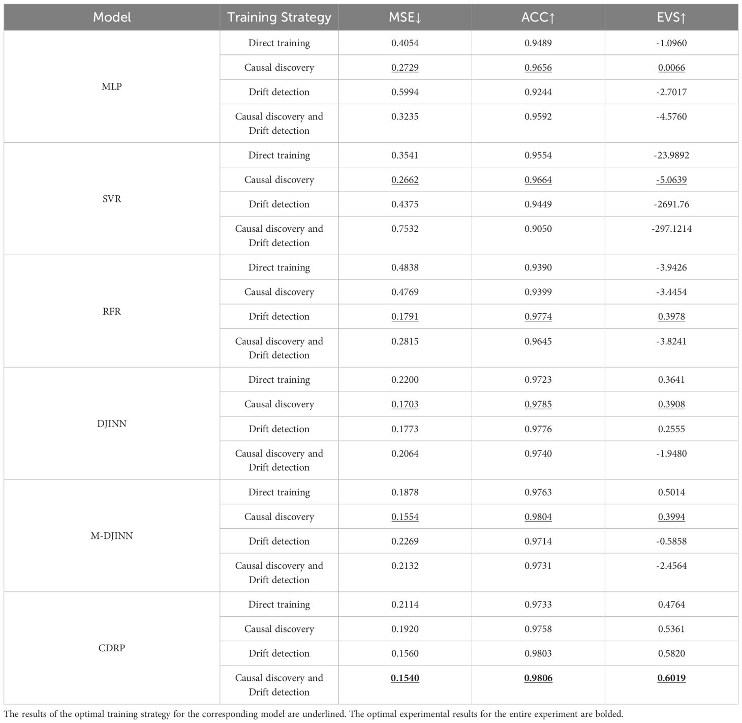
Table 2 Performance of the selected models with different training strategies.

To validate the effectiveness of removing interference from weakly associated elements and concept drift detection on the improvement of RuleFit’s precision in the MDOC inversion tasks, RuleFit was trained using both direct training and training with a combination of causal discovery and concept drift detection. Figure 5 shows the variation curves of MSE, ACC, and EVS. It’s evident that the utilization of causal discovery and concept drift detection notably reduced MSE, while at the same time increasing ACC and EVS. Models enhanced with causal discovery and concept drift detection demonstrated significant early-stage optimization in MSE and ACC around 15 to 18 weeks, compared to the RuleFit model that underwent direct training. The EVS also showed an increase after the final training session was completed. This convincingly confirms the superiority of CDRP in elevating the precision for MDOC inversion task.

Figure 5

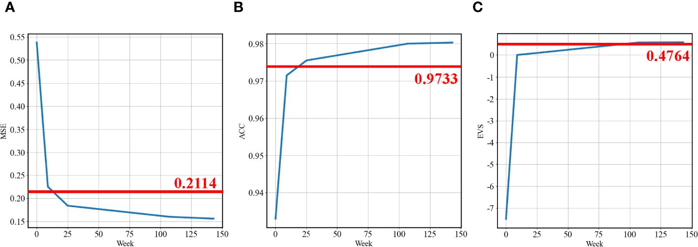
Figure 5 Performance of CDRP and directly trained RuleFit. (A)MSE; (B)ACC; (C)EVS. (The blue line represents the metric change of CDRP, while the solid red line represents the metric of directly trained RuleFit.).

For an intuitive analysis of CDRP’s fitting effect, the RuleFit model, trained with a combination of causal discovery and concept drift detection, was used to process the entire dataset. The comparison between predicted and observed MDOC values is presented through overlay plot and scatter plot (Figure 6). Figure 6A displays a notable consistency between predicted and observed MDOC values. Meanwhile, Figure 6B reveals that the predictions for a significant portion of data points lie within the orange area, which signifies the range of Root Mean Square Error (RMSE). From the analysis, it can be concluded that CDRP demonstrates commendable fitting efficacy, rendering it applicable for real-world MDOC inversion task.

Figure 6

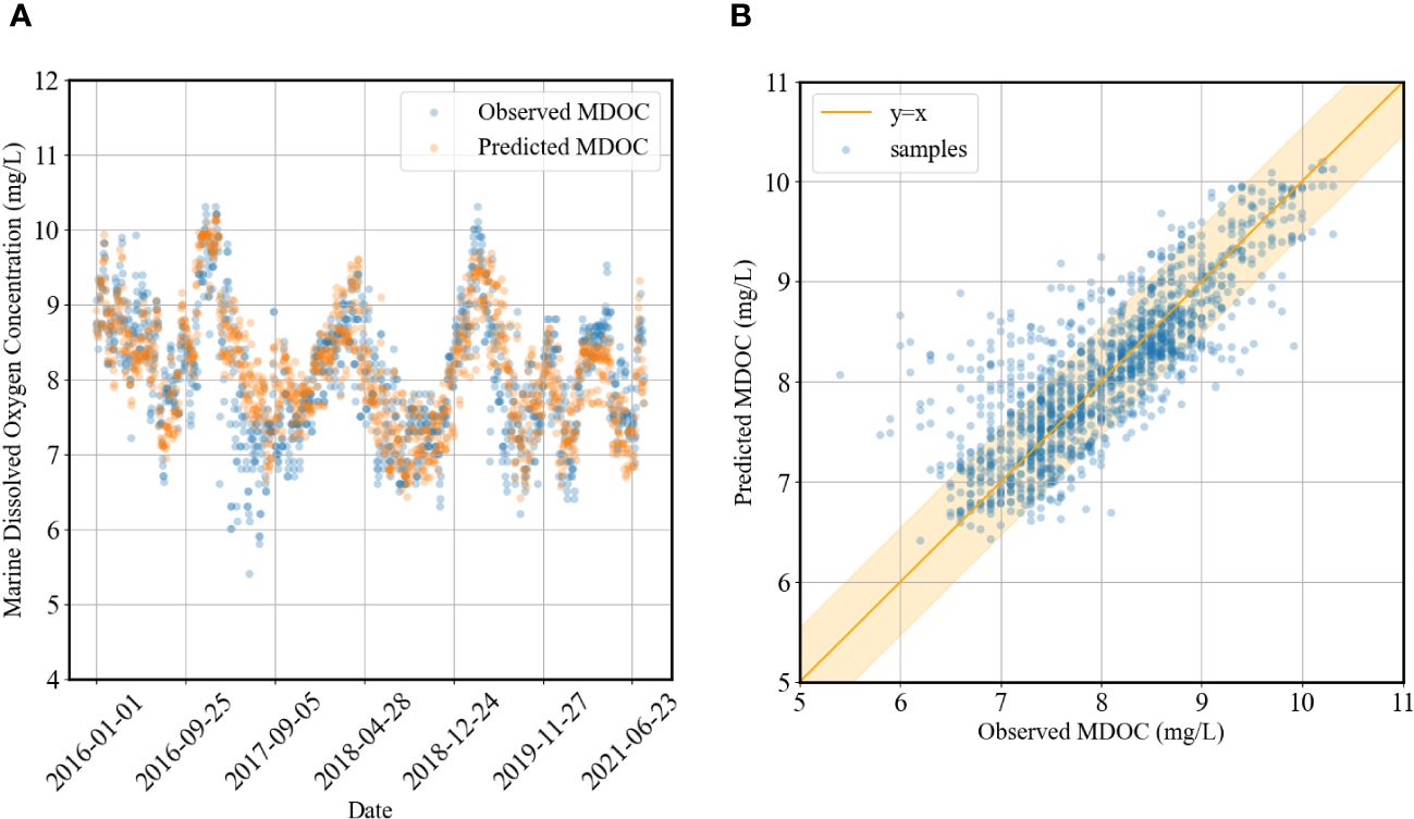
Figure 6 Comparison of the predicted and observed MDOC, using overlay plot (A) and scatter plot (B). (Orange line in scatter plot is the fitted linear between observed and predicted values).

3.2 Interpretation of inversion results

3.2.1 Causal discovery

To analyze the correlation between marine elements from the causal perspective, we employ the PCMCI causal discovery algorithm to conduct causal analysis on the initially selected five elements (OTMP, SAL, CLCON, PH, and TURB) with the target element MDOC. Figure 7A shows the causal relationship graph between marine elements, while Figure 7B displays the causal relationship graph from the perspective of time series, highlighting the two-day delay between temperature (OTMP) and MDOC. In addition to the direct causal influence from pH to MDOC, chlorophyll concentration (CLCON) indirectly affects MDOC through OTMP. All of them indicate that pH, OTMP and CLCON are key elements in MDOC inversion. Additionally, a notable causal link exists from MDOC to salinity (SAL), which is supported by the subsequent SHAP analysis. Finally, we can conclude that turbidity (TURB) has almost no causal relationship with MDOC. This conclusion is reinforced by the experiments described in Section 3.1, which shows that removing weakly associated turbidity effectively reduces interference in the MDOC inversion task.

Figure 7

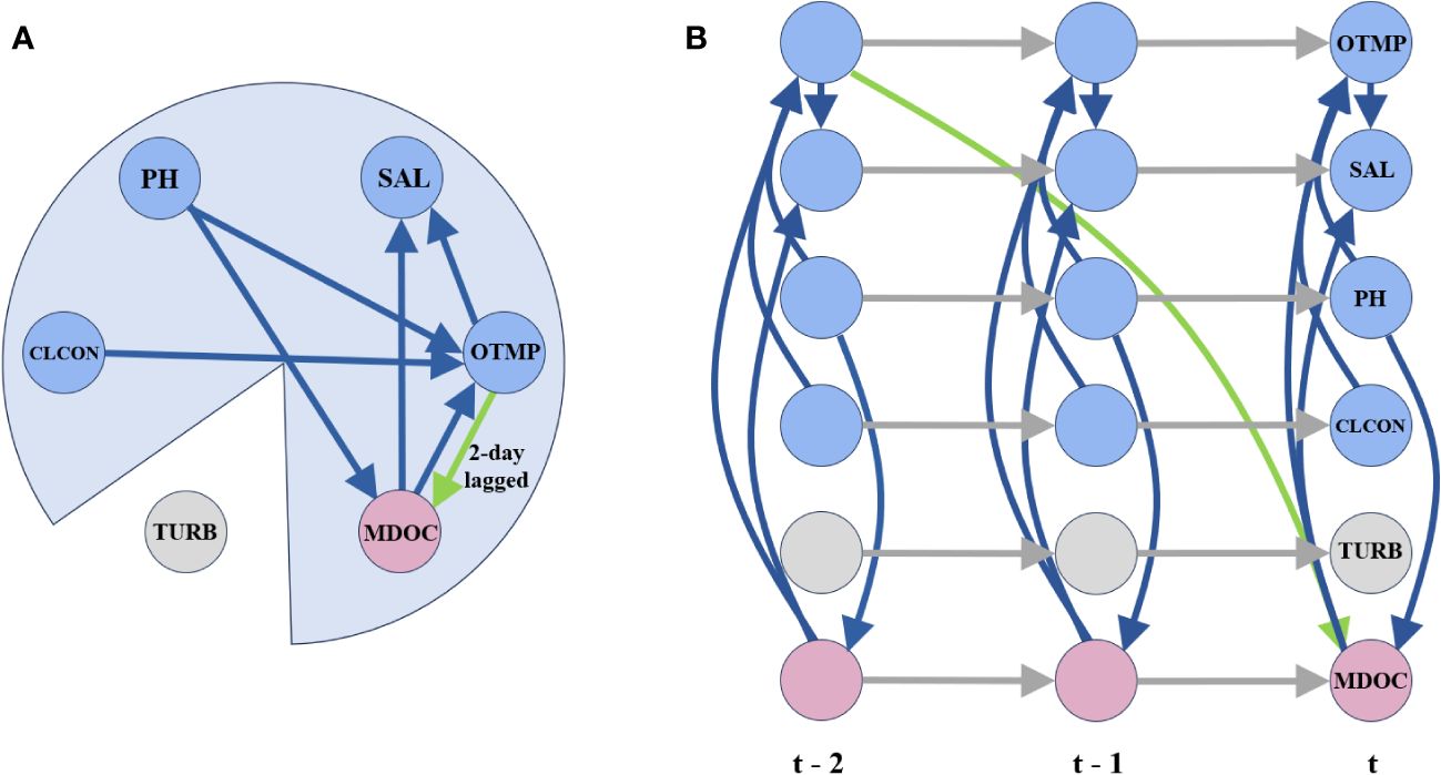
Figure 7 Causal relationships between marine elements. (A) Causal relationship graph; (B) Time series graph.

3.2.2 Rulefit rule extraction

RuleFit, composed of a series of readily interpretable IF-THEN rules and linear adjustments, not only demonstrates significant precision in inversion tasks but also enables initial insights into the operational mechanisms of the intelligent inversion. This is achieved through the extraction and subsequent analysis of critically significant rules. The primary rules extracted by RuleFit are detailed in Table 3. By analyzing the judgments on specific elements within the primary rules, we conclude the following insights: (i) An increase in temperature is inversely related to MDOC, as shown by rules 3 and 4; (ii) Salinity mostly has a negative impact on MDOC, as depicted by rules 1, 2 and 3; (iii) A decrease in pH is related with a reduction in MDOC, as specified by rule 1 and 4; (iv) An elevation in chlorophyll concentration is positively linked to MDOC, as illustrated by rules 2.

Table 3

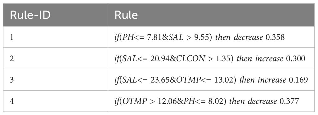
Table 3 The main rules extracted through RuleFit.

3.2.3 SHAP analysis

To understand the operational mechanisms of the intelligent inversion model from a global perspective, SHAP analysis was utilized to quantify the impact magnitude and direction of the marine elements on the climatological normals of MDOC. We present a summary plot of the SHAP analysis for selected marine elements (Figure 8). In this plot, the vertical axis orders the marine elements by their impact magnitude, and the horizontal axis shows the change (Shapley value) to the MDOC climatological normals (7.98 mg/L) based on the values of these marine elements. The color of the dots is detailed in the legend to the right of the plot, while the vertical stacking of dots illustrates the frequency of sample points with specific values. Figure 8 shows that salinity has the largest impact on MDOC climatological normals, with a trend suggesting that lower salinity leads to a higher positive impact on MDOC climatological normals. This is consistent with the results of RuleFit rule extraction analysis. The influence of pH on MDOC climatological normals is secondary, primarily indicating a positive impact at higher pH levels. Lower temperatures are associated with a greater positive impact on the MDOC climatological normals. The impact of chlorophyll concentration on MDOC climatological normals is the smallest, primarily manifested as a negative effect.

Figure 8

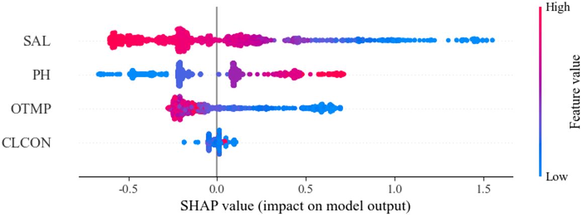
Figure 8 Summary plot for marine elements.

To investigate the interaction between salinity, which contributes most significantly to the impact on MDOC climatological normals, and other elements, we conducted SHAP analysis and produced dependence plots (Figure 9). Preliminary analysis of Figure 9 allows us to deduce that salinity exerts a positive impact on the MDOC climatological normals when below approximately 25 psu, and manifests a negative impact when exceeding this threshold. The increase in temperature reduces the positive impact of salinity (Figure 9A), while an increase in pH elevates the positive impact of salinity (Figure 9B). Conversely, chlorophyll concentration does not exhibit a significant effect on the impact of salinity (Figures 9C).

Figure 9

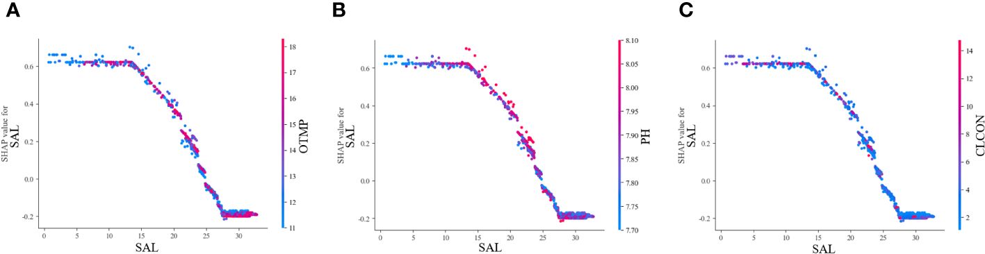
Figure 9 Dependence plot of the interaction between SAL and other marine elements. (A) OTMP; (B) pH; (C) CLCON.

3.2.4 LIME analysis

Contrary to the SHAP analysis method, which focuses on assessing the global contributions of marine elements, LIME analysis can provide local interpretation for the influencing factors of various marine elements at key climate nodes, and the critical value range can guide the quantitative judgment of the impact direction of input elements on the output target element — MDOC, thereby providing local interpretation schemes and enhancing the interpretability of the overall framework. We selected three consecutive dates of MDOC minima (Figures 10A-C) and three consecutive dates of MDOC maxima (Figures 10D-F) to analyze the impact direction and magnitude of each marine elements within their respective value ranges at these critical climate nodes. We referenced the research by El Bilali et al. (2023) in our analysis, identifying the critical value ranges at which the direction of the influence of marine elements on the MDOC climatological normals changes. The analysis provides the following insights: (i) Salinity has the most significant impact on MDOC climatological normals, followed by pH in typical cases, with temperature being less significant, and chlorophyll concentration having the least impact; (ii) Salinity below 23.81 psu has a positive impact on the MDOC climatological normals, while levels above 29.70 psu have a negative impact; (iii) Temperatures below 12.64°C have a positive effect on the MDOC climatological normals, whereas temperatures above it have a negative effect; (iv) pH above 7.80 positively impacts the MDOC climatological normals, while pH below it has a negative impact; (v) Chlorophyll concentrations above 5.50 µg/L positively affect the MDOC climatological normals, whereas in other circumstances a negative impact occurs.

Figure 10

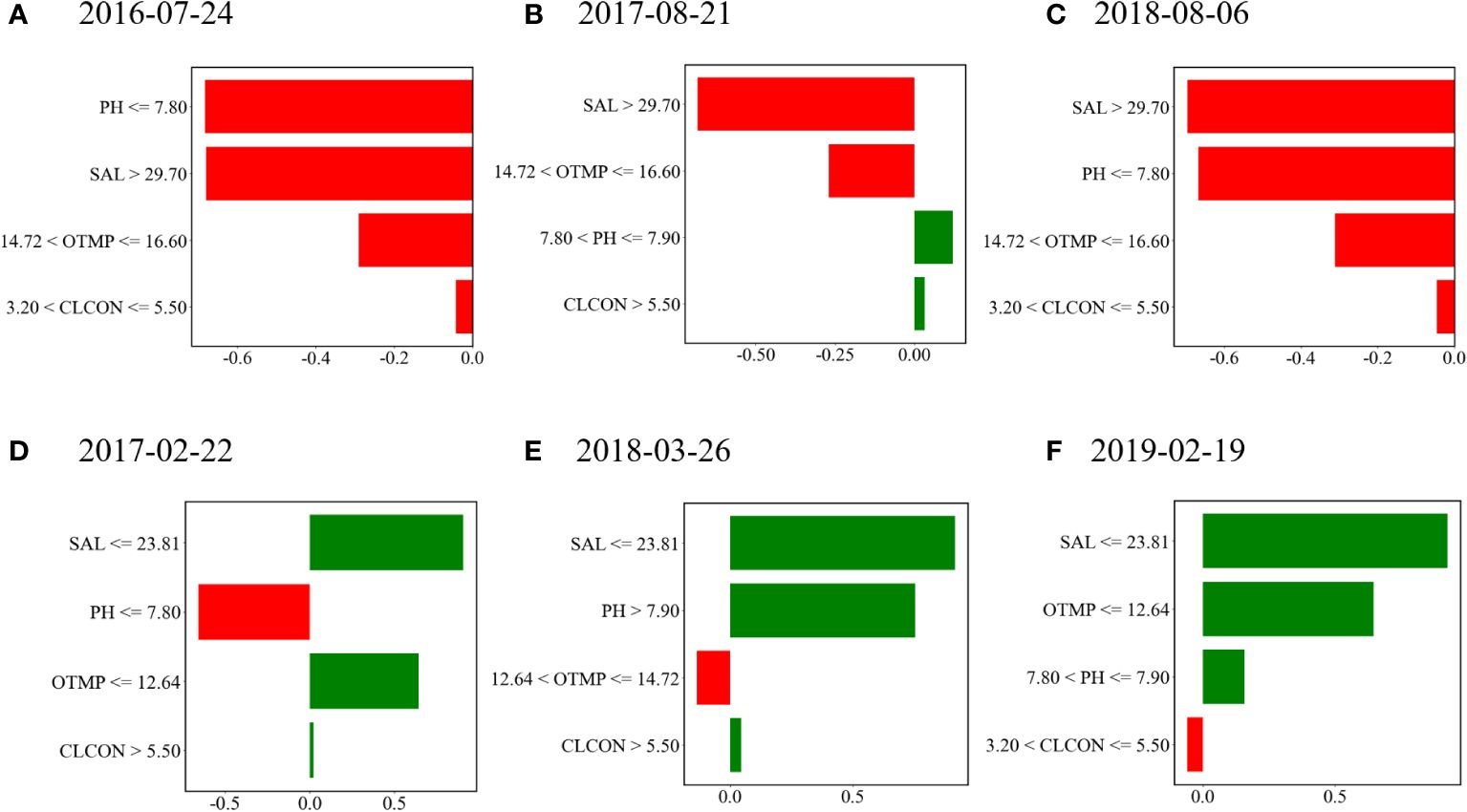
Figure 10 (A–F) The impact of marine elements at the extrema of MDOC. Negative LIME values indicate MDOC below historical median while positive LIME values indicate MDOC above historical median.

4 Discussion

MDOC is one of the primary indicators in the domain of marine ecology. In this study, we applied a series of artificial intelligence models to the MDOC inversion task, where our proposed framework CDRP demonstrated optimal precision. SVR is sensitive to the characteristics of input data, while RFR is susceptible to overfitting. Moreover, complex models such as MLP, DJINN, and its modified version M-DJINN require large volumes of data for effective training. Conversely, the RuleFit model creates a broad set of predictive rules tailored for the inversion task. This method offers deep insights into the computational mechanisms of inversion and exhibits strong generalization abilities, as evidenced in (Luo et al., 2022). Overall, CDRP which utilizes the RuleFit model achieves superior precision in inversion task.

4.1 Precision influenced by causal discovery and concept drift

We introduced causal discovery and concept drift detection during the training process. By analyzing the experimental results (Table 2), it can be found that causal discovery significantly improves the inversion performance of all models. It follows that causal discovery can keenly identify uncorrelated elements, which can guide the improvement of model training strategies. However, concept drift detection only achieves a boost in effectiveness in tree-based algorithms, which demonstrates a kind of compatibility between them. By expanding to other tree-based algorithms, it is still possible to improve model performance while extracting key features of the dataset. Finally, CDRP achieves optimal performance by simultaneously introducing causal discovery and concept drift detection in training process. However it may be not the optimal training strategy for all models. Causal discovery involves input feature-level reduction from the perspective of causal inference, while concept drift detection involves time series-level reduction from the perspective of data distribution changes. This could potentially lead to excessive reduction and result in model underfitting.

4.2 Interpretability

In the literature on applying AI models to MDOC inversion task, there is a lack of exploration on interpretability. This can lead to risks associated with unknown computational logic. Therefore, enhancing the interpretability of the MDOC inversion task is of significant importance. To solve this problem, we constructed an interpretive process of “causal discovery + rules analysis + post hoc analysis + literature validation of consistency” to comprehensively improve the interpretability of the MDOC inversion process.

4.2.1 Causal discovery

To investigate the causal relationships between each marine element and MDOC, we introduced PCMCI to conduct causal discovery on temperature, salinity, pH, chlorophyll concentration, turbidity, and MDOC. By estimating the strength and directionality of causal relationships among highly interdependent time series of multiple marine elements, we found that PCMCI can effectively eliminate the interference of weakly correlated marine elements on model learning. After causal analysis, the causal graph and time series causal graph are shown in Figure 7. By analyzing the correlation with MDOC, we can classify the marine elements into four categories: direct causal association (temperature, pH), indirect causal association (chlorophyll concentration), correlated association (salinity), and weakly correlated association (turbidity). Among these, temperature belongs to the category of time lagged causal correlation. Specifically, the temperature from two days ago has a direct causal effect on the current MDOC. The global warming and ocean acidification are direct factors leading to the occurrence of marine hypoxia, which is consistent with the results of causal graph analysis (Breitburg et al., 2018; George et al., 2024). The promoting effect of chlorophyll on MDOC is essentially achieved through biomass influencing temperature, thus resulting in a positive correlation effect on MDOC (MacPherson et al., 2007; Li et al., 2024a). Although salinity is not a causal parent of MDOC, the causal relationship between MDOC and salinity makes this correlation relationship indispensable in the MDOC inversion task. Furthermore, the subsequent SHAP analysis further confirms the importance of salinity. Ultimately, turbidity does not exhibit significant causal relationship with other marine elements. Therefore, the presence of this element would bring negative interference to the MDOC inversion task. The quantitative experiments conducted earlier demonstrate that removing the interference from the turbidity significantly contributes to improving the accuracy level of MDOC inversion. This further elucidates the importance and necessity of introducing causal discovery method for enhancing interpretability.

4.2.2 Rules analysis

To analyze the influence of marine elements on the MDOC climatological normals from the model inference perspective, the RuleFit model was introduced. By establishing a large initial set of predictive rules and then refining these rules to improve inversion precision, this method achieves high-precision and also helps understand how the model works. This understanding comes from utilizing and interpreting the set of rules. The decrease in MDOC with higher temperature is due to increased oxygen demand and reduced oxygen solubility as temperature rise (Breitburg et al., 2018; Ye et al., 2021, 2023; Bandara et al., 2024). Silva et al. (2009) described Equatorial Subsurface Water (ESSW) characteristics, noting that the highest underwater salinity values are associated with the lowest MDOC and high nitrate and phosphate levels. This supports the idea that colder, less saline water can dissolve more (Kouketsu et al., 2022; Sun et al., 2023), which matches the RuleFit rule showing an inverse relationship between salinity and MDOC. The research by Schmitt et al. (2008) shows long-range correlations between pH and MDOC in their power-law spectrum, particularly noting that ocean acidification goes along with marine hypoxia (Gao et al., 2020; George et al., 2024). This supports the RuleFit finding that a lower pH results in decreased MDOC. The rule that an increase in chlorophyll concentration leads to higher MDOC is supported by (MacPherson et al., 2007; Li et al., 2024a), indicating that higher chlorophyll concentration produce more oxygen indirectly, thereby increasing MDOC. Therefore, it can be concluded that the RuleFit model utilized in CDRP extracts rules that are easily interpretable with high precision, and this approach is well-supported by a wealth of marine scientific literature.

4.2.3 Post-hoc analysis

SHAP analysis is employed to enhance the understanding of the MDOC inversion process by examining its results. This analysis, conducted from a global perspective, explores how marine elements contribute to the MDOC inversion task. Additionally, a local interpretability analysis through LIME is utilized to analyze the model’s computational basis at MDOC extrema. SHAP and LIME analyses show that marine elements can affect MDOC climatological normals positively or negatively at different times. Seasonal changes in MDOC are influenced by sunlight, ice cover, air temperature, winds, and currents (Kroeker et al., 2020; Xu et al., 2022). Events like upwelling, which brings colder deep seawater with lower MDOC content to the surface, also cause short-term MDOC variations (Booth et al., 2012; Chen et al., 2022; Castrillón-Cifuentes et al., 2023; Wang et al., 2023a). The conclusion drawn from the SHAP analysis that salinity is negatively correlated with MDOC is consistent with RuleFit analysis. Furthermore, the findings about temperature’s negative impact and pH’s positive impact on salinity contributions agree with previous analysis based on RuleFit rules. Moreover, LIME analysis identifies the critical value range for salinity’s impacts as 23.81–29.70 psu. This range includes zero Shapley value of salinity from SHAP analysis (around 25 psu, as shown in Figure 9), confirming the consistency between SHAP and LIME analysis on salinity. Similarly, LIME provides the direction of impact (positive, negative, positive) and critical value ranges for pH, temperature and chlorophyll concentration on the MDOC climatological normals (7.80, 12.64°C, 5.50 µg/L), respectively.

4.2.4 Insight from interpretability analysis

Post-hoc analysis has led to findings that align with causal discovery and RuleFit rules, and they also offer specific critical value ranges. These findings provide marine scientists with quantitative insights into how various marine elements influence the magnitude and direction of changes in MDOC climatological normals. Based on insights from interpretability analysis, we can propose several strategies to reduce marine hypoxia. The finding that salinity negatively impacts MDOC indicates that reducing sewage discharge could help prevent deoxygenation in the ocean, especially near coastlines. Similarly, limiting greenhouse gas emissions to slow down global warming and ocean acidification is also an effective strategy. Moreover, maintaining marine ecological indicators within reasonable ranges is crucial for controlling dissolved oxygen levels.

5 Conclusion

This paper introduces an interpretable artificial intelligence framework CDRP designed for high-precision MDOC inversion. Initially, PCMCI is utilized for causal discovery of marine elements and to eliminate the interference of weakly associated elements. Following that, key frame data is selected through concept drift detection, resulting in the formation of the training dataset. Subsequently, the dataset is fed into the rule-based RuleFit model for training. This step is followed by extracting operational rules, which enables the establishment of an initial interpretation. Afterwards, an advanced analysis is conducted utilizing post-hoc analysis techniques, specifically SHAP and LIME. This comprehensive approach offers insights that are consistent with actual marine observation, especially in terms of their influence on the MDOC climatological normals. In comparative tests with SVR, RFR, MLP, DJINN, and M-DJINN, our framework showed the best performance in precision and interpretability. The principal findings from the analysis of research results are as follows: (i) Conducting causal discovery of marine elements through PCMCI, along with removing weakly associated elements and analyzing causal relationships, can effectively enhance the effectiveness and interpretability of model learning. (ii) Using concept drift detection to capture changes in marine elements effectively enhances the precision and interpretability based on data reduction of CDRP. (iii) Considering RuleFit, SHAP, and LIME analysis results together, the ranking of the influence of marine elements on MDOC climatological normals is: salinity > pH > temperature > chlorophyll concentration. (iv) The critical value ranges for the impact on climatological normals are salinity (23.81-29.70 psu), pH (7.80), temperature (12.64°C) and chlorophyll concentration (5.50 µg/L). In summary, CDRP demonstrates high precision and interpretability in single-point measured MDOC inversion tasks, displaying commendable consistency with conclusions in marine literature on MDOC.

Currently, considering the expansion of remote sensing data sources, exploring computational techniques that improve both precision and interpretability with this data is seen as a promising field for academic research. Furthermore, a more valuable interpretation of concept drift phenomena can be achieved through deep involvement in causal analysis. Therefore, conducting further analysis at the moment when concept drift occurs through methods such as causal discovery and causal effect analysis represents a highly prospective research direction.

Data availability statement

Publicly available datasets were analyzed in this study. This data can be found here: https://www.ndbc.noaa.gov/historical_data.shtml.

Author contributions

XL: Writing – original draft, Writing – review & editing, Conceptualization, Data curation, Formal analysis, Funding acquisition, Investigation, Methodology, Resources, Validation, Visualization. ZL: Writing – original draft, Writing – review & editing, Data curation, Investigation, Software, Validation. ZY: Writing – review & editing, Software, Supervision, Validation. FM: Writing – review & editing, Methodology, Supervision, Validation. TS: Writing – review & editing, Conceptualization, Data curation, Funding acquisition, Investigation, Methodology, Resources, Supervision, Validation.

Funding

The author(s) declare financial support was received for the research, authorship, and/or publication of this article. This work was supported by grants of National Key Research and Development Project of China (Project No. 2021YFA1000103), the Natural Science Foundation of Shandong Province of China (Project No. ZR2020MF140) and the Key Laboratory of Marine Hazard Forecasting, Ministry of Natural Resources (Project No. LOMF2202).

Conflict of interest

The authors declare that the research was conducted in the absence of any commercial or financial relationships that could be construed as a potential conflict of interest.

Publisher’s note

All claims expressed in this article are solely those of the authors and do not necessarily represent those of their affiliated organizations, or those of the publisher, the editors and the reviewers. Any product that may be evaluated in this article, or claim that may be made by its manufacturer, is not guaranteed or endorsed by the publisher.

Footnotes

1. ^ https://archimer.ifremer.fr/doc/00187/29825/
2. ^ https://www.ncei.noaa.gov/products/world-ocean-database
3. ^ https://www.ndbc.noaa.gov/historicaldata.shtml

References

Atitey K., Motsinger-Reif A. A., Anchang B. (2024). Model-based evaluation of spatiotemporal data reduction methods with unknown ground truth through optimal visualization and interpretability metrics. Briefings Bioinf. 25, bbad455. doi: 10.1093/bib/bbad455

CrossRef Full Text | Google Scholar

Bandara R. M. W. J., Curchitser E., Pinsky M. L. (2024). The importance of oxygen for explaining rapid shifts in a marine fish. Global Change Biol. 30, e17008. doi: 10.1111/gcb.17008

CrossRef Full Text | Google Scholar

Bénard C., Biau G., Da Veiga S., Scornet E. (2021). “Interpretable random forests via rule extraction,” in International Conference on Artificial Intelligence and Statistics (PMLR). Microtome Publishing31: USA. 937–945.

Google Scholar

Booth J. A. T., McPhee-Shaw E. E., Chua P., Kingsley E., Denny M., Phillips R., et al. (2012). Natural intrusions of hypoxic, low ph water into nearshore marine environments on the california coast. Continent. Shelf Res. 45, 108–115. doi: 10.1016/j.csr.2012.06.009

CrossRef Full Text | Google Scholar

Breitburg D., Levin L. A., Oschlies A., Grégoire M., Chavez F. P., Conley D. J., et al. (2018). Declining oxygen in the global ocean and coastal waters. Science 359, eaam7240. doi: 10.1126/science.aam7240

PubMed Abstract | CrossRef Full Text | Google Scholar

Brock A. L., Kostadinova K., Mørk-Pedersen E., Hensel F., Zhang Y., Valverde-Pérez B., et al. (2023). Remediation of marine dead zones by enhancing microbial sulfide oxidation using electrodes. Mar. pollut. Bull. 193, 115142. doi: 10.1016/j.marpolbul.2023.115142

PubMed Abstract | CrossRef Full Text | Google Scholar

Carrazana-Escalona R., Andreu-Heredia A., Moreno-Padilla M., Reyes del Paso G. A., Sánchez- Hechavarría M. E., Muñoz-Bustos G. (2022). Blood pressure prediction using ensemble rules during isometric sustained weight test. J. Cardiovasc. Dev. Dis. 9, 440. doi: 10.3390/jcdd9120440

PubMed Abstract | CrossRef Full Text | Google Scholar

Castrillón-Cifuentes A. L., Zapata F. A., Wild C. (2023). Physiological responses of pocillopora corals to upwelling events in the eastern tropical pacific. Front. Mar. Sci. 10. doi: 10.3389/fmars.2023.1212717

CrossRef Full Text | Google Scholar

Chakraborty D., Başağaoğlu H., Winterle J. (2021). Interpretable vs. noninterpretable machine learning models for data-driven hydro-climatological process modeling. Expert Syst. Appl. 170, 114498. doi: 10.1016/j.eswa.2020.114498

CrossRef Full Text | Google Scholar

Chen C.-C., Ko D. S., Gong G.-C., Lien C.-C., Chou W.-C., Lee H.-J., et al. (2022). Reoxygenation of the hypoxia in the east China sea: A ventilation opening for marine life. Front. Mar. Sci. 8. doi: 10.3389/fmars.2021.787808

CrossRef Full Text | Google Scholar

Conley D. J., Carstensen J., Ærtebjerg G., Christensen P. B., Dalsgaard T., Hansen J. L., et al. (2007). Long-term changes and impacts of hypoxia in danish coastal waters. Ecol. Appl. 17, S165–S184. doi: 10.1890/05-0766.1

CrossRef Full Text | Google Scholar

El Bilali A., Abdeslam T., Ayoub N., Lamane H., Ezzaouini M. A., Elbeltagi A. (2023). An interpretable machine learning approach based on dnn, svr, extra tree, and xgboost models for predicting daily pan evaporation. J. Environ. Manage. 327, 116890. doi: 10.1016/j.jenvman.2022.116890

PubMed Abstract | CrossRef Full Text | Google Scholar

Friedman J. H., Popescu B. E. (2008). Predictive learning via rule ensembles. Ann. Appl. Stat 2, 916–954. doi: 10.1214/07-AOAS148

CrossRef Full Text | Google Scholar

Gao K., Gao G., Wang Y., Dupont S. (2020). Impacts of ocean acidification under multiple stressors on typical organisms and ecological processes. Mar. Life Sci. Technol. 2, 279–291. doi: 10.1007/s42995-020-00048-w

CrossRef Full Text | Google Scholar

George R., Job S., Semba M., Monga E., Lugendo B., Tuda A. O., et al. (2024). High-frequency dynamics of ph, dissolved oxygen, and temperature in the coastal ecosystems of the tanga-pemba seascape: implications for upwelling-enhanced ocean acidification and deoxygenation. Front. Mar. Sci. 10. doi: 10.3389/fmars.2023.1286870

CrossRef Full Text | Google Scholar

Giglio D., Lyubchich V., Mazloff M. R. (2018). Estimating oxygen in the southern ocean using argo temperature and salinity. J. Geophys. Res.: Oceans 123, 4280–4297. doi: 10.1029/2017JC013404

CrossRef Full Text | Google Scholar

Hutchins D. A., Capone D. G. (2022). The marine nitrogen cycle: new developments and global change. Nat. Rev. Microbiol. 20, 401–414. doi: 10.1038/s41579-022-00687-z

PubMed Abstract | CrossRef Full Text | Google Scholar

Ji X., Shang X., Dahlgren R. A., Zhang M. (2017). Prediction of dissolved oxygen concentration in hypoxic river systems using support vector machine: a case study of Een-Rui Tang river, China. Environ. Sci. pollut. Res. 24, 16062–16076. doi: 10.1007/s11356-017-9243-7

CrossRef Full Text | Google Scholar

Jiang Y., Gou Y., Zhang T., Wang K., Hu C. (2017). A machine learning approach to argo data analysis in a thermocline. Sensors 17, 2225. doi: 10.3390/s17102225

PubMed Abstract | CrossRef Full Text | Google Scholar

Jin X., Gruber N. (2003). Offsetting the radiative benefit of ocean iron fertilization by enhancing n2o emissions. Geophys. Res. Lett. 30. doi: 10.1029/2003GL018458

CrossRef Full Text | Google Scholar

Johnson K. S., Plant J. N., Coletti L. J., Jannasch H. W., Sakamoto C. M., Riser S. C., et al. (2017). Biogeochemical sensor performance in the soccom profiling float array. J. Geophys. Res.: Oceans 122, 6416–6436. doi: 10.1002/2017JC012838

CrossRef Full Text | Google Scholar

Karadurmus U., Sari M. (2022). Marine mucilage in the sea of Marmara and its effects on the marine ecosystem: mass deaths. Turkish J. Zool. 46, 93–102. doi: 10.3906/zoo-2108–14

CrossRef Full Text | Google Scholar

Kouketsu S., Murata A., Arulananthan K. (2022). Subsurface water property structures along 80 e under the positive Indian ocean dipole mode in december 2019. Front. Mar. Sci. 9. doi: 10.3389/fmars.2022.848756

PubMed Abstract | CrossRef Full Text | Google Scholar

Kroeker K. J., Bell L. E., Donham E. M., Hoshijima U., Lummis S., Toy J. A., et al. (2020). Ecological change in dynamic environments: Accounting for temporal environmental variability in studies of ocean change biology. Global Change Biol. 26, 54–67. doi: 10.1111/gcb.14868

CrossRef Full Text | Google Scholar

Li H., Li X., Song D., Nie J., Liang S. (2024a). Prediction on daily spatial distribution of chlorophylla in coastal seas using a synthetic method of remote sensing, machine learning and numerical modeling. Sci. Total Environ. 910, 168642. doi: 10.1016/j.scitotenv.2023.168642

PubMed Abstract | CrossRef Full Text | Google Scholar

Li Y., Robinson S. V., Nguyen L. H., Liu J. (2023b). Satellite prediction of coastal hypoxia in the northern gulf of Mexico. Remote Sens. Environ. 284, 113346. doi: 10.1016/j.rse.2022.113346

CrossRef Full Text | Google Scholar

Li X., Wang Z., Chen C., Tao C., Qiu Y., Liu J., et al. (2024b). Semid: Blind image inpainting with semantic inconsistency detection. Tsinghua Sci. Technol. 29, 1053–1068. doi: 10.26599/TST.2023.9010079

CrossRef Full Text | Google Scholar

Li X., Wang F., Song T., Meng F., Zhao X. (2023a). Astmen: an adaptive spatiotemporal and multi-element fusion network for ocean surface currents forecasting. Front. Mar. Sci. 10. doi: 10.3389/fmars.2023.1281387

CrossRef Full Text | Google Scholar

Lu J., Liu A., Dong F., Gu F., Gama J., Zhang G. (2018). Learning under concept drift: A review. IEEE Trans. knowledge Data Eng. 31, 2346–2363. doi: 10.1109/TKDE.2018.2876857

CrossRef Full Text | Google Scholar

Luo C., Li S., Zhao Q., Ou Q., Huang W., Ruan G., et al. (2022). Rulefit-based nomogram using inflammatory indicators for predicting survival in nasopharyngeal carcinoma, a bi-center study. J. Inflammation Res. 15, 4803–4815. doi: 10.2147/JIR.S366922

CrossRef Full Text | Google Scholar

MacPherson T. A., Cahoon L. B., Mallin M. A. (2007). Water column oxygen demand and sediment oxygen flux: patterns of oxygen depletion in tidal creeks. Hydrobiologia 586, 235–248. doi: 10.1007/s10750-007-0643-4

CrossRef Full Text | Google Scholar

Matear R., Hirst A. (2003). Long-term changes in dissolved oxygen concentrations in the ocean caused by protracted global warming. Global Biogeochem. Cycles 17. doi: 10.1029/2002GB001997

CrossRef Full Text | Google Scholar

Mollas I., Bassiliades N., Tsoumakas G. (2022). Conclusive local interpretation rules for random forests. Data Min. Knowledge Discovery 36, 1521–1574. doi: 10.1007/s10618-022-00839-y

CrossRef Full Text | Google Scholar

Naik V., Manjappa S. (2011). Mathematical modeling for dissolved oxygen prediction in mixing zone–a case study. J. Environ. Sci. Eng. 53, 429–436.

PubMed Abstract | Google Scholar

Ribeiro M. T., Singh S., Guestrin C. (2016). ““ why should i trust you?” explaining the predictions of any classifier,” in Proceedings of the 22nd ACM SIGKDD international conference on knowledge discovery and data mining. ASSOC Computing Machinery 1515: NEW YORK USA. 1135–1144. doi: 10.1145/2939672.2939778

CrossRef Full Text | Google Scholar

Ross A. C., Stock C. A. (2019). An assessment of the predictability of column minimum dissolved oxygen concentrations in chesapeake bay using a machine learning model. Estuarine Coast. Shelf Sci. 221, 53–65. doi: 10.1016/j.ecss.2019.03.007

CrossRef Full Text | Google Scholar

Runge J., Nowack P., Kretschmer M., Flaxman S., Sejdinovic D. (2019). Detecting and quantifying causal associations in large nonlinear time series datasets. Sci. Adv. 5, eaau4996. doi: 10.1126/sciadv.aau4996

PubMed Abstract | CrossRef Full Text | Google Scholar

Schmitt F. G., Dur G., Souissi S., Zongo S. B. (2008). Statistical properties of turbidity, oxygen and ph fluctuations in the seine river estuary (France). Phys. A: Stat. Mech. its Appl. 387, 6613–6623. doi: 10.1016/j.physa.2008.08.026

CrossRef Full Text | Google Scholar

Silva N., Rojas N., Fedele A. (2009). Water masses in the humboldt current system: Properties, distribution, and the nitrate deficit as a chemical water mass tracer for equatorial subsurface water off Chile. Deep Sea Res. Part II: Topical Stud. Oceanogr. 56, 1004–1020.

Google Scholar

Štrumbelj E., Kononenko I. (2014). Explaining prediction models and individual predictions with feature contributions. Knowledge Inf. Syst. 41, 647–665. doi: 10.1007/s10115-013-0679-x

CrossRef Full Text | Google Scholar

Sun Y.-J., Robinson L. F., Parkinson I. J., Stewart J. A., Lu W., Hardisty D. S., et al. (2023). Iodine-to-calcium ratios in deep-sea scleractinian and bamboo corals. Front. Mar. Sci. 10. doi: 10.3389/fmars.2023.1264380

CrossRef Full Text | Google Scholar

Suntharalingam P., Sarmiento J. L., Toggweiler J. (2000). Global significance of nitrous-oxide production and transport from oceanic low-oxygen zones: A modeling study. Global Biogeochem. Cycles 14, 1353–1370. doi: 10.1029/1999GB900100

CrossRef Full Text | Google Scholar

Wan K., Tanioka K., Shimokawa T. (2023). Rule ensemble method with adaptive group lasso for heterogeneous treatment effect estimation. Stat Med. 42, 3413–3442. doi: 10.1002/sim.9812

PubMed Abstract | CrossRef Full Text | Google Scholar

Wang L., Jiang Y., Qi H. (2020). Marine dissolved oxygen prediction with tree tuned deep neural network. IEEE Access 8, 182431–182440. doi: 10.1109/ACCESS.2020.3028863

CrossRef Full Text | Google Scholar

Wang Y., Yuan X., Bi H., Ren Y., Liang Y., Li C., et al. (2023a). Understanding arctic sea ice thickness predictability by a markov model. J. Climate 36, 1–40. doi: 10.1175/JCLI-D-22–0525.1

CrossRef Full Text | Google Scholar

Wang Y., Yuan X., Ren Y., Bushuk M., Shu Q., Li C., et al. (2023b). Subseasonal prediction of regional antarctic sea ice by a deep learning model. Geophys. Res. Lett. 50, e2023GL104347. doi: 10.1029/2023GL104347

CrossRef Full Text | Google Scholar

Xu W., Fleddum A. L., Shin P. K., Sun J. (2022). Impact of and recovery from seabed trawling in soft-bottom benthic communities under natural disturbance of summer hypoxia: A case study in subtropical hong kong. Front. Mar. Sci. 9. doi: 10.3389/fmars.2022.1010909

PubMed Abstract | CrossRef Full Text | Google Scholar

Yang W., Li Z., Liu M., Lu Y., Cao K., Maciejewski R., et al. (2020). “Diagnosing concept drift with visual analytics,” in 2020 IEEE conference on visual analytics science and technology (VAST) (IEEE). IEEE Computer Soc: Los Alamitos, CA, USA. 12–23. doi: 10.1109/VAST50239.2020.00007

CrossRef Full Text | Google Scholar

Ye M., Li B., Nie J., Wen Q., Wei Z., Yang L.-L. (2023). Graph convolutional network assisted sst and chl-a prediction with multi-characteristics modeling of spatio-temporal evolution. IEEE Trans. Geosci. Remote Sens. 61. doi: 10.1109/TGRS.2023.3330517

CrossRef Full Text | Google Scholar

Ye M., Nie J., Liu A., Wang Z., Huang L., Tian H., et al. (2021). Multi-year enso forecasts using parallel convolutional neural networks with heterogeneous architecture. Front. Mar. Sci. 8, 717184. doi: 10.3389/fmars.2021.717184

CrossRef Full Text | Google Scholar

Zhang G., Hóu Z., Huang Y., Shi J., Bride H., Dong J. S., et al. (2023). Extracting optimal explanations for ensemble trees via automated reasoning. Appl. Intell. 53, 14371–14382. doi: 10.1007/s10489-022-04180-1

CrossRef Full Text | Google Scholar