Movement and diving behavior of satellite-tagged male sperm whales in the Gulf of Alaska

Wild, Lauren A.; Mueter, Franz J.; Straley, Jan M.; Andrews, Russ D.

doi:10.3389/fmars.2024.1394687

ORIGINAL RESEARCH article

Front. Mar. Sci., 03 September 2024

Sec. Marine Megafauna

Volume 11 - 2024 | https://doi.org/10.3389/fmars.2024.1394687

Movement and diving behavior of satellite-tagged male sperm whales in the Gulf of Alaska

Lauren A. Wild^1,2*

Franz J. Mueter¹

Jan M. Straley²

Russ D. Andrews³

¹College of Fisheries and Ocean Sciences, University of Alaska Fairbanks, Juneau, AK, United States
²Applied Fisheries and Department of Biology, University of Alaska Southeast, Sitka, AK, United States
³Marine Ecology & Telemetry Research, Seabeck, WA, United States

Male sperm whales (Physeter macrocephalus) are known to interact with and depredate from commercial longline fishing vessels targeting sablefish (Anoplopoma fimbria) in the Gulf of Alaska (GOA). This study aims to better understand their movement patterns and diving behavior in this region, and in relation to depredation behavior. Between 2007 and 2016 a total of 33 satellite tags were deployed on sperm whales interacting with fishing vessels in the eastern GOA. A subset of these tags also collected dive characteristics. We used state space models to interpolate hourly positions from tags and estimate behavioral state from 29 usable tag records, 14 of which had associated dive information. Whales exhibited slower horizontal movement (1.4 km/hr) within GOA waters compared to south of the GOA (5.5 km/hr), indicating tagged whales sped up when they left the region. Behavioral states indicated primarily foraging behavior (82% of locations) in the GOA and primarily transiting behavior (74% of locations) when whales left the GOA. Dive data showed average ( ± Standard Deviation) maximum dive depths of 396 m ( ± 166), and dive durations of 32 min (± 9). Generalized additive models indicated that dives were significantly deeper and longer during the daytime than dawn, dusk, or nighttime, and dives were significantly deeper and shorter during quarter moons, when tidal currents are weakest. Maximum dive depth decreased in areas of higher sablefish CPUE, suggesting a potential link between the sablefish fishery and depredation behavior. As seafloor depth increased, up to 800 m, dives became deeper, indicating that whales were likely targeting both bathypelagic and mesopelagic prey. This highlights the importance of the GOA continental slope as a foraging ground for male sperm whales. This enhanced understanding of sperm whale foraging ecology informs management and conservation efforts in high latitude foraging grounds.

1 Introduction

Sperm whales (Physeter macrocephalus) are a deep diving marine predator whose movement, population dynamics, and stock structure are poorly understood throughout much of their worldwide range. In the United States (US), they are listed as endangered under the Endangered Species Act (ESA) of 1973, and depleted under the Marine Mammal Protection Act (MMPA) of 1972 (Muto et al., 2018). Management of sperm whales in US waters is often hindered by a lack of reliable data on regional stock structure and population dynamics, which is important in establishing recovery plans required by both ESA and MMPA listings. Females, juveniles, and calves are thought to inhabit warmer equatorial waters, while mature males move to higher latitude foraging grounds (Rice, 1989; Whitehead, 2003), though the movement and timing of movements between these areas are not well studied. In fact, movement of males has been identified as one of the largest knowledge gaps in global understanding of sperm whales (Whitehead, 2003). It is thought that in these high latitude foraging grounds, males are usually found in small bachelor groups or alone (Caldwell et al., 1966; Best, 1979; Reeves et al., 1985; Rice, 1989).

The Gulf of Alaska (GOA) represents a high latitude foraging ground of male sperm whales. In the North Pacific and GOA, sperm whales were heavily exploited during commercial whaling through the 1970’s (Mizroch and Rice, 2013; Ivashchenko and Clapham, 2014). The effects of this exploitation on patterns of occurrence and stock structure of sperm whales is not known. There are currently three genetically distinct stocks recognized in the North Pacific: Alaska, California Current, and Hawaii (Mesnick et al., 2011). Genetic analysis has also shown that the males that make up the Alaska stock originate from multiple lower latitude populations (Mesnick et al., 2011). There is acoustic evidence that sperm whales are present year-round in the GOA, though incidences of detections are 70% higher in summer months compared to winter months (Mellinger et al., 2004; Diogou et al., 2019).

In their GOA foraging grounds, sperm whales are known to remove fish from commercial longline fishing gear targeting sablefish (Anoplopoma fimbria), a fishery that takes place primarily in offshore waters over the continental slope habitat in water depths of 150 to 900 m (Hill et al., 1999; Sigler et al., 2008). This removal, known as depredation, incurs economic costs to the fishery, increases risk of entanglement for whales, and impacts the NOAA Fisheries annual stock assessment survey (Hill et al., 1999; Sigler et al., 2008; Straley et al., 2015; Peterson and Hanselman, 2017; Hanselman et al., 2018). Since 2003 the Southeast Alaska Sperm Whale Avoidance Project (SEASWAP) has been studying sperm whale depredation in the GOA, with a goal to minimize interactions (Straley et al., 2015). Using fishing vessels as a platform for research, this collaboration between fishermen, scientists, and managers has been successful in gaining important insights into the interactions of sperm whales with fishing vessels in the GOA. SEASWAP has found that sperm whales engaging in depredation in the GOA are male (Mesnick et al., 2011; Straley et al., 2015), and that they are attracted to the distinct acoustic pattern of propeller cavitation made when longline fishing vessels haul their gear (Thode et al., 2007; Wild et al., 2017). Catch-per-unit-effort (CPUE) data show that fishing sets with higher CPUE were also associated with higher presence of whales, while fishers that experienced low CPUE often experienced no depredation, suggesting that the whales are also able to track areas of high fish abundance (Straley et al., 2015). It also suggests that sperm whale movements in this region are tied to fishing activity in addition to finding natural prey resources.

Foraging behavior and movement of male sperm whales in high latitudes is difficult to observe because of the remoteness, high costs of conducting fieldwork, and difficult weather and oceanic conditions in these regions. Much of the work that has been done focuses on acoustic studies using animal-borne suction-cupped archival tags to assess fine-scale movement and acoustic activity during foraging dives (Madsen et al., 2002a, b; Miller et al., 2004; Watwood et al., 2006; Teloni et al., 2008; Guerra et al., 2017). These studies have focused on echolocation signals corresponding to dive behavior over short time windows of hours instead of days, and with small sample sizes. While acoustic and behavioral archival tags can help elucidate fine-scale foraging tactics of individuals, inferring population-level movements over longer periods of time and over broader regions is difficult with these short-duration data sets. Few studies have specifically assessed regional-level movements and habitat use by males foraging at high latitudes, coupled with diving and foraging behavior.

Individual movement of sperm whales is primarily centered around energetic requirements needed to grow, survive, and reproduce. Tracking individual movements and characterizing behavior can be used to better understand biological processes that influence food availability and occurrence of animals in general (Gurarie et al., 2016; Hays et al., 2016). In turn, this information can be used by managers to designate critical habitat, conservation zones and stock boundaries for highly migratory species, such as sperm whales. In the marine environment prey resources are often patchy due to complex interactions among environmental variables (e.g. sea surface temperature, tidal currents, light availability, bathymetry, etc.). Identifying the key environmental drivers influencing predator movement and habitat use can be used to predict changes in distribution due to a changing environment (Jay et al., 2012; Joy et al., 2015). However, observing these behaviors can be difficult for some species such as sperm whales, because they are often distributed far from shore, undertake deep dives that can last more than 30 minutes, and are often hard to locate and track (Watwood et al., 2006). Furthermore, surface observations rarely allow for visual confirmation of foraging habits, social interactions, or other ecological markers. Satellite telemetry through transmitting tags can be used to track more broad-scale movements, capture migratory routes, and elucidate foraging hotspots.

Argos satellite-linked transmitting tags can be used in the marine environment to gain valuable insight into broad movement patterns, how animals interact with their environment, and specific environmental characteristics that influence their behavior and occurrence (McConnell and Fedak, 1996; Hays et al., 2004; Ropert-Coudert and Wilson, 2005). Satellite tagging can provide researchers with detailed movement patterns to determine spatiotemporal foraging patterns and infer the quality of the environment that was visited by the tagged animals (Bailey et al., 2012; Bestley et al., 2013; Guinet et al., 2014; Thorne et al., 2017). SEASWAP has used satellite tags to gain information on how sperm whales use their GOA foraging ground habitats through assessment of 11 satellite tag records deployed in the summers of 2007 and 2009 in the eastern GOA (Straley et al., 2014). Sperm whale movements were found to be strongly associated with the continental slope, with horizontal movement rates increasing when whales moved south out of Alaskan waters (Straley et al., 2014).

Interpreting movement data for marine mammals is complicated by the fact that they are underwater for most of their lives and tags only transmit when the animal is at the surface to breathe; therefore, transmissions occur at irregular intervals due to the diving behavior of the animal. Tag placement on the animal, behavioral and physical heterogeneity of individual animals, and occurrence of a satellite passing overhead while the animal is at the surface contribute to high variability in position estimates and associated error. A common way to deal with these data gaps and variable error among position estimates is to interpolate positions at a fixed interval using modeling techniques such as state space models (SSM) (Jonsen et al., 2005). SSMs are a stochastic model-based approach to working with tag data that is designed to address measurement error, and separate the observation error inherent in the Argos system from the often random processes determining animal movement (Tanizaki, 2001; Jonsen et al., 2003, 2005, 2007; Aarts et al., 2008). They are a natural framework to apply to animal movement in that they estimate the state of an unobserved process (tagged animal movement and space use) from an observed data set (surface intervals that produce estimated positions from Argos data). SSMs rely on the notion of an animal’s “state”, or behavior, which can be categorized into classes such as “moving/transiting” and Area-Restricted Search (ARS). ARS behavior is often referred to as a “foraging” or “resident” state, and we will refer to it in this study as “foraging”.

In the current study, we increase the sample size of SEASWAP’s satellite tag data set and expand the analysis to deal with the error associated with position estimates through state space modeling. We interpolate uncertain positions obtained from satellite tags to estimate positions at regularly spaced time intervals and estimate underlying behavioral states of sperm whales in this region. In addition, we add dive behavior data from a subset of satellite tags equipped with depth sensors to quantify correlations between environmental drivers and diving behavior. Our goal was to better understand depredating male sperm whales’ use of space in the GOA using satellite telemetry. Specific objectives were to: 1) describe general patterns in sperm whale movements and diving behavior; 2) characterize foraging and transiting behavior to identify foraging hotspots of sperm whales in the GOA; and 3) identify environmental predictors of sperm whale diving behavior during their presence in the GOA.

2 Materials and methods

2.1 Field deployments

Satellite tags were deployed along the eastern GOA slope and in Chatham Strait between Cape Ommaney (56.15°N, 134.67°W), and Cross Sound (58.08°N, 136°W) between 2007 and 2016, roughly corresponding to the SEASWAP study area of the eastern GOA (Figure 1). Most tag deployment effort occurred in June and July, though deployments ranged from May 3 to September 17 for any given year (Table 1). All tags were deployed from small vessels at a distance of 3-15 m from the whale using one of two methods: between 2007 and 2009 tags were deployed using a crossbow; from 2010 to 2016 tags were deployed using a pneumatic rifle (DAN-INJECT JM SP 25, DanWild LLC) (Supplementary Material S1). During tagging operations we attempted to take photographs of dorsal fins and flukes (Whitehead and Gordon, 1986) to identify the individual whale in the SEASWAP catalog and ensure the same whales were not repeatedly approached and tagged in a single year. All tagged whales were determined to be male either from genetic samples collected from the individual or based on size as determined by the tagging team. Tag IDs were given the prefix “SWsat” for “sperm whale satellite tag”, followed by a numeric indicator assigned in chronological order based on date/time of tag deployment, while identification of individual whales to the SEASWAP photographic-identification (photo-ID) catalog was listed as the “Whale ID”.

Figure 1

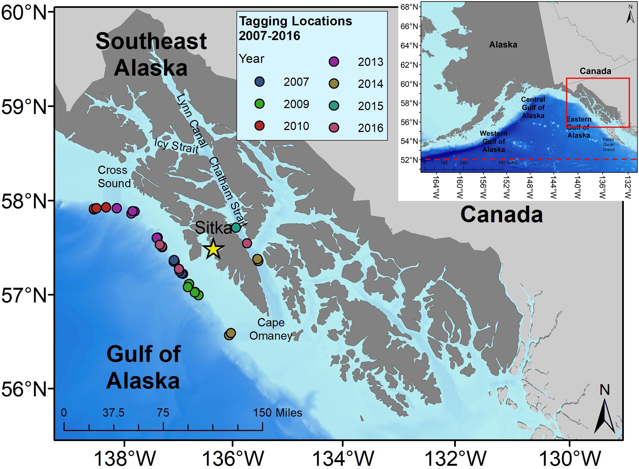
Figure 1. Locations, represented by red dots, where sperm whales (n=33 tags on 29 individuals) were tagged in the eastern Gulf of Alaska (GOA) study area, 2007-2016. The study area is depicted by the shaded box. Full map of the Gulf of Alaska shows dashed line at 52° N latitude boundary of the Gulf of Alaska, and red box around the Southeast Alaska region. The star shows the location of Sitka, Alaska, where the work was based.

Table 1

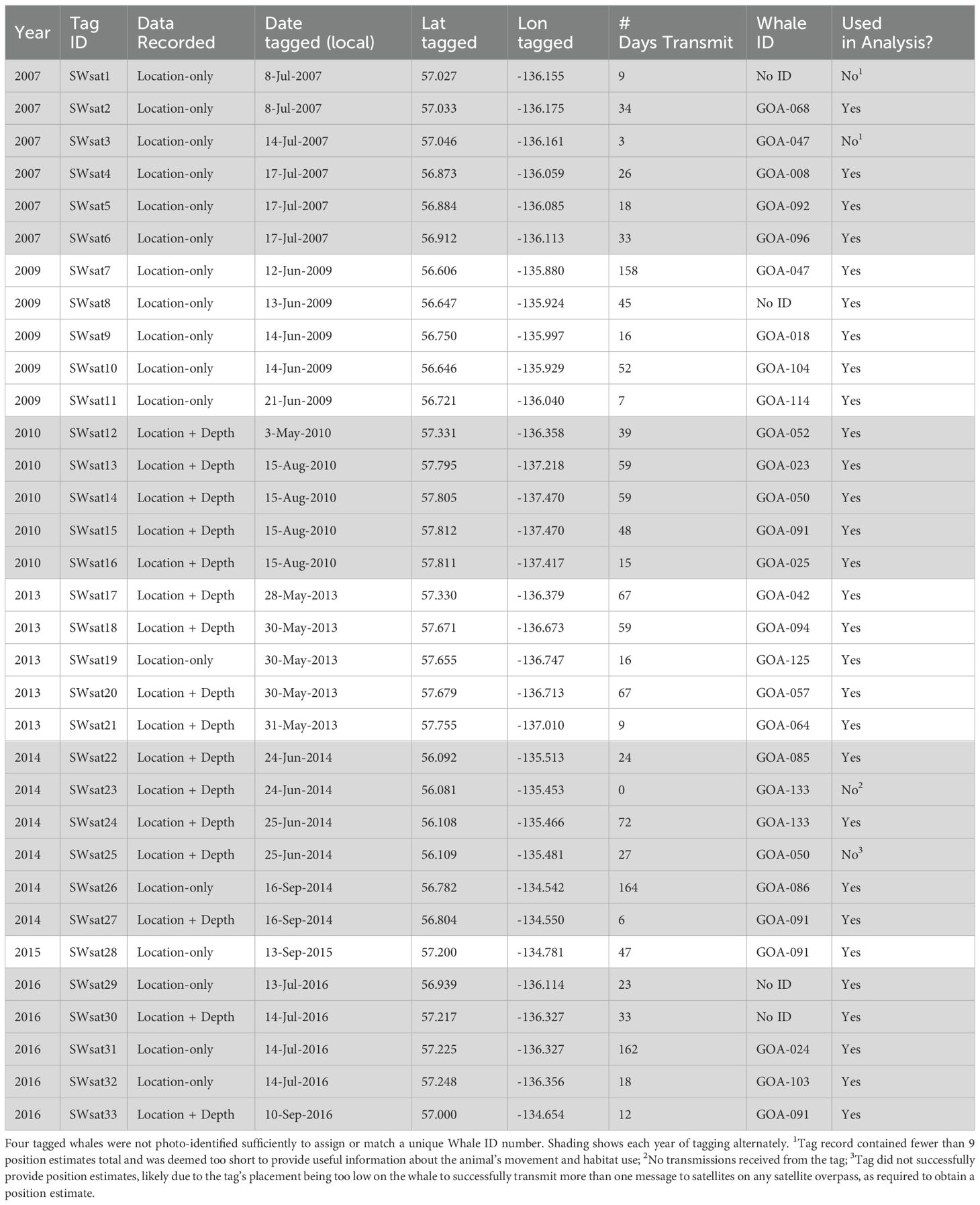
Table 1. Summary of deployment data for 33 satellite tags placed on sperm whales by SEASWAP between 2007-2016.

2.2 Tag programming

A variety of tag types were used throughout the study, all configured as Low Impact Minimally Percutaneous External-Electronics Transmitters (LIMPET) (Andrews et al., 2008) (Wildlife Computers, Redmond, WA) (Table 1). All tags transmitted location information, while some tags also contained a pressure sensor, which recorded and transmitted dive information in addition to locations (Table 1). Tag size varied, with a maximum dimension of 5.5 x 5.0 x 2.7 cm and maximum weight of 57 g; two barbed titanium darts penetrated the skin and outer blubber layer up to 6.8 cm (Andrews et al., 2008).

Tags transmitted to polar-orbiting satellites via the Argos satellite system. Tag programming parameters varied among years due to different project goals and objectives, and because tags evolved and improved over the years. In general, tags transmitted every day for between 19 and 50 days, before switching to a duty cycle to save battery life, transmitting every 2 to 4 days for 10 to 40 days. Thereafter, tags continued to transmit on one day out of every 5 to 10 days for the remainder of the tag attachment duration.

A subset of tags deployed between 2010 and 2016 also contained a pressure sensor to record and transmit depth information during dives (Mk10-A and SPLASH tags, Table 1). These tags were programmed to collect and transmit dive data according to a duty cycle that varied with the year of deployment and SEASWAP project objectives. A full description of dive data is available in the Supplementary Material. In general, tags were programmed to transmit summaries of position and depth data for the first 20 days, before switching to a duty cycle, during which they transmitted data only from the dates of transmission. Duty cycles consisted of tags transmitting every 2 to 4 days for the first 10 to 30 days, and then every 8 to 16 days for the remainder of the tag deployment. Dive depths were collected from a pressure sensor on the tag, sampled at a resolution of 0.5 Hz for tags in 2010 (SWsat12-16) and 1 Hz for all other tags (2013-2016) (Supplementary Material S1). Tags summarized the dive data in two ways, sending messages summarizing daily histograms of maximum dive depths, providing an accurate count of how many dives were performed each day, and as Behavior Log data that summarized the duration, maximum depth reached and shape for individual dives. Maximum dive depth was defined as the maximum depth reached in an individual dive. Start and end times of dives were determined using a wet/dry sensor, and dive information was collected on dives that qualified as “dives” according to a qualifying threshold of at least 30 m depth and 30 sec in length. The dive depth threshold was chosen to separate surface intervals and shallow silent dives from foraging dives, with the 30 m threshold equating to approximately two body lengths of an adult male sperm whale. Once a whale crossed the dive qualifying threshold for both depth and duration, the record was classified as a dive and dive characteristics were recorded and transmitted when the tag was at the surface. Dive characteristics were summarized by the tag as: start and end time of the dive, maximum depth of the dive, duration of the dive, and dive shape. Dive shape was assigned to each dive based on the relationship between bottom time and dive duration and classified as either V-shaped, U-shaped, or square-shaped (Supplementary Material S1).

2.3 Satellite location filtering

All position estimates from satellite tags were derived by Argos using the Doppler effect to calculate a position. Positions were then filtered to assess each position estimate and remove improbable positions from the data set using the Douglas Argos-Filter, v. 7.06 (Andrews et al., 2008; Douglas et al., 2012). Prior to 2011, a non-linear Least-Squares algorithm was provided by Service Argos to calculate raw position estimates. In 2012, Argos began offering a new processing algorithm, the more robust Kalman smoothing method, which improved location accuracy, especially when a limited number of messages were received (Lopez and Malardé, 2011; Lopez et al., 2014; Silva et al., 2014). Tag data from 2009 and 2010 were re-processed by Argos using the Kalman smoothing method, thus only 2007 position estimates were calculated using the Least-Squares algorithm.

Most position estimates from Argos have an associated location quality class (LC) associated with them, which is linked to the estimated error from each position estimate and is referred to as the radius of error, forming an ellipse around the position. These LC’s consist of 3, 2, 1, A, B, and Z, with 3 being the most precise estimate of position (i.e. the smallest error associated with the position estimate) with a <250 m error radius, and B being the least accurate with unbounded accuracy estimation (CLS, 2016). LC codes of “Z” denote invalid positions, and these positions were removed from the data set prior to analysis.

2.4 Modelling locations using SSMs

We used a first difference correlated random walk model (DCRW) to fit sperm whale movement from the final tag data set. SSMs were fit using a hierarchical version of Bayesian switching state space modelling methods to predict locations of whales at regularly spaced time intervals and to estimate behavioral state (Jonsen et al., 2005; Jonsen, 2016). We interpolated irregularly spaced location data by regularly spaced time steps, restricting models to the period of time when tags transmitted daily. Time steps over which to interpolate data should be chosen considering both: 1) the relevant timescale over which behavioral changes are likely to be evident; and 2) the actual temporal resolution of the data. For the latter, the tag data produced an average of 12 position estimates per day, or an approximately two-hour time step. For the former, behavioral changes could occur at timescales of an hour or two as animals search for prey but given that sperm whale dives can last nearly an hour, behavioral changes may not be evident at time steps less than three or four hours. Finally, small time steps also result in a higher degree of autocorrelation of positions when analyzing movement data. We experimented with time steps of 1-6 hours and used model diagnostics to ultimately select three-hour time steps to estimate behavioral states, bridging the gap between the temporal resolution of the tag data (12 position estimates every day equating to a 2-hour time step) and the temporal resolution that behavioral changes would likely be evident (every three or four hours) with reduced autocorrelation of the data. Hourly time steps to estimate positions (but not behavioral states) from the models were also used in dive behavior analysis, due to their increased sample size and good agreement with position estimates from the three-hour time step. We did not estimate positions after tags switched to a less than daily duty cycle due to increased uncertainty when irregular data becomes even more sparse.

Models were fit using the ‘bsam’ package version 1.1.3 (Jonsen et al., 2005; Jonsen, 2016) in R version 4.0.3 (R Core Team, 2019). The package uses the software JAGS (Depaoli et al., 2016) through an interface to R provided by the package “rjags” version 4.10 (Plummer, 2016). Three Markov Chain Monte Carlo (MCMC) chains were run in parallel for 50,000 simulations, first discarding 25,000 samples from the ‘burn-in’ phase. Samples were then thinned, retaining every 200^th sample to reduce autocorrelation. Behavioral mode (b) was returned by the model as a value between 1 and 2, where values close to 1 (b < 1.25) were interpreted as being indicative of transiting behavior and values close to 2 (b > 1.75) were indicative of area-restricted-search (foraging behavior) (Jonsen et al., 2005, 2007).

For the subset of tags that included dive statistics (n=14), hourly tag position estimates were matched to the closest dive if the time of the position estimate was within five minutes of the start or end of a dive, or during the dive. If position estimates were matched to a dive, they were associated with the maximum dive depth, dive duration, and dive shape information for further analysis.

2.5 Environmental data

In order to better understand the potential mechanisms, influences, and patterns behind the diving behavior of whales, environmental variables at each dive location were assessed. Seafloor depths for each dive position estimate were obtained from the NOAA Alaska Fisheries Science Center’s Central Gulf of Alaska raster, collected from lead-line and single-beam echosounder soundings from 225 National Ocean Service hydrographic surveys and compiled as a 100 m resolution ArcMap grid (https://www.fisheries.noaa.gov/alaska/ecosystems/alaska-bathymetry-sediments-and-smooth-sheets). For data points that were outside of the area covered by the NOAA bathymetry surface (approximately 30% of the data points), the Pacific GEBCO_19 gridded surface was used, which contains depths in a bathymetric raster surface in ArcGIS (GEBCO, 2019) with a grid resolution of 15-arc seconds, or approximately 500 m.

Habitat was categorized into one of three categories: continental shelf, continental slope, and deep ocean basin. Continental shelf habitat was defined as nearshore depths between 0-300 m, continental slope was defined as the area where the continental slope drops off to the deep ocean basin with depths between 300 – 2000 m, and the deep ocean basin was defined as having depths greater than 2000 m (Weingartner et al., 2009).

Slope of the bathymetry was calculated over a 1 nautical mile gridded area in the eastern GOA that roughly corresponded to the NOAA Fisheries Eastern GOA statistical area for sablefish management, from 53°N Latitude to 60°N Latitude (https://www.fisheries.noaa.gov/alaska/sustainable-fisheries/pacific-halibut-and-sablefish-individual-fishing-quota-ifq-program). Slope calculations were conducted in GIS using the slope tool in the Spatial Analyst Tools toolbox, with output specified in degrees, using a z-factor conversion of 0.00001625 for latitudes around 56°N. Interpolated positions from the movement models were then matched to grid cells and the slope was extracted from that cell.

Catch-per-unit-effort (CPUE) data for estimating local sablefish abundance was obtained from fishery observers on commercial longline fishing vessels participating in the sablefish fishery in the Southeast (SE) area of the GOA within the broader Eastern GOA statistical area, collected and compiled by the NOAA Fisheries Ted Stevens Marine Research Institute in Juneau, AK. Data represented catches from 1995 through 2017. A geospatial model of CPUE was developed in a generalized additive modeling (GAM) framework, which was used to predict CPUE over the interpolated sperm whale position estimates from SSMs within our study area in the eastern GOA (see Supplementary Material S2). We assumed that spatial patterns in CPUE were consistent over the time frame of the data set, reflecting a long-term average CPUE at each position (Supplementary Material S2).

Lunar phase was calculated as a continuous variable of lunar illumination from the ‘lunar’ package in R for each interpolated hourly tag position. For lunar illumination, 0 represents a new moon, 0.5 represents quarter moon, 1 represents a full moon (100% illumination), crescent moons are between 0 and 0.5, and gibbous moons are between 0.5 and 1. Diel cycle was calculated for each hourly tag position as well, using the R package ‘maptools’, as day, night, dawn, or dusk. Nautical dawn/dusk were defined as starting or ending, respectively, when the angle of the sun was 12 degrees below the horizon.

2.6 Statistical summaries and analyses

2.6.1 Objective 1: describe general patterns in sperm whale movement and diving behavior

Broad patterns of horizontal movement and summary statistics on sperm whale tags were described for each tagged whale. Average movement speeds, the number of days tags transmitted data, and the general direction of movement were summarized, as well as any unique movements or tag tracks. Whale tracks were analyzed with respect to their movement in and out of the GOA, which we define as the region northward of 52° N Latitude, which coincides roughly with Queen Charlotte Sound and the southern end of Haida Gwaii, British Columbia (Figure 1) (Brower et al., 1988). In addition, dive behavior was summarized using the maximum depth, maximum duration, and an estimate of dive shape for each dive.

Minimum horizontal rates of travel (km/hr) and minimum daily distance (km) traveled were estimated as in Straley et al. (2014) to quantify daily movements. Briefly, straight-line distances between the best position estimate (based on Argos LC) for each day were first calculated using great circle distance methods, and then divided by the time between those estimates to get a minimum daily movement rate (km/hr). If more than one position estimate had the same quality code, the first position of the day with the highest code was chosen. While the straight-line daily distance method does not account for all of the movement by the tagged animal (e.g. back-and-forth or circuitous foraging movement throughout a day), nor vertical movement during dives, it provides an estimate of the minimum rate of movement or minimum swimming speed required to travel between the most accurate daily positions. The minimum rate of horizontal movement was multiplied by 24 hr to provide a minimum estimate of the distance traveled that day.

2.6.2 Objective 2: characterize foraging and transiting behavior to identify foraging hotspots of sperm whales in the GOA

Foraging and transiting behavioral states were quantified from SSMs and filtered to only include data points where behavioral states (b) had a high degree of certainty, 1<b<1.25 and 1.75<b<2 (Jonsen et al., 2013; Jonsen, 2016). Foraging and transiting behavioral states for each whale position were examined visually to see if we could identify foraging hotspots of sperm whales in the GOA. Spatial patterns in the predicted foraging behavior were visualized by smoothing the probability of foraging across individuals using a spatial binomial model of presence (1) or absence (0). Probabilities were estimated using a tensor product smooth of latitude and longitude as implemented in the R package ‘mgcv’ (Wood, 2017) with the amount of smoothing chosen subjectively to have approximately 50 equivalent degrees of freedom. The proportion of transiting versus foraging states produced by the model was calculated for each whale, and paired t-tests were used to examine whether the proportions were different within the GOA from those outside the GOA. Specifically, based on previous research we hypothesized that whales were spending more time foraging within the GOA than outside the GOA. We also tested for differences in dive shape within and outside the GOA using a Pearson’s Chi-squared test. Square dives provide the greatest bottom time, where we presume most foraging is happening. Therefore, we hypothesized that dives performed when the whale was in a “foraging” state were more likely to be square than when in the “transiting” state. Given we presume sperm whales spend time in the GOA primarily to feed, we hypothesized that square dives would be more prevalent in the GOA than outside the GOA.

2.6.3 Objective 3: identify environmental drivers of diving behavior

To explore environmental drivers of diving behavior we restricted our analysis to the eastern GOA (Figure 1) to exclude areas to the south that may serve different purposes for sperm whales (i.e. migration). Moreover, CPUE data for sablefish to use as a covariate in the model were only available for this area. Thus, we clipped the SSM output to include only positions (interpolated from SSMs) within the GOA, removing 26% of the full data set. We further filtered the data to include only tag data for positions that had associated dive information, further reducing the data set by 40% and resulting in 5,090 data points used in the final analysis for this objective.

For the subset of tags that included diving data, we assessed the influence of environmental covariates on sperm whale diving behavior using generalized additive mixed effects models (GAMMs) fit via maximum likelihood estimation, with Tag ID as the random effect (Wood, 2017). For this analysis we used response variables of maximum dive depth and dive duration. Response variables were modeled as a function of seafloor depth (z), seafloor slope, lunar cycle (lunar), diel cycle (diel), day of the year (DOY), and an index of local sablefish abundance estimated from the fishery (Catch-per-unit-effort, CPUE) as follows:

\begin{matrix} y_{i, s, t} = α + a_{i} + f_{1} (z_{s}) + f_{2} (s l o p e_{s}) + f_{3} (l u n a r_{t}) + f_{4} (d i e l_{t}) \\ + f_{5} (d o y_{t}) + f_{6} (C P U E_{s}) + f_{7} (l a t_{s}, l o n_{s}) + ϵ_{i, s, t} \end{matrix}

where y_i,s,t is the response (maximum dive depth or dive duration) for tag i at position s and time t, α is an overall intercept, a_i is a random intercept for tag i to allow for individual variation in dive depth and duration, z_s is seafloor depth at position s, f₁-f₆ are smooth functions with up to 3 degrees of freedom to restrict relationships to ecologically plausible functional forms, f₇ is a bivariate smoother to account for any remaining spatial variation, and ϵ is the residual variation. The random effects a_i and residuals $ϵ_{i, s, t}$ are assumed to be normally distributed with mean zero and variance σ_a² and σ_ϵ², respectively.

A histogram of maximum dive depths across all tagged whales showed multiple modes, with a minor mode of shallow dives between 30 m (our dive depth qualifying threshold) and approximately 125 m, a main mode between 125 and 800 m, and a broad mode of relatively few deep dives ranging from 800 m to the maximum dive depth. All of the deeper dives were produced by a small subset of four whales, while the maximum dive depths of most whales were less than 800 m. Initial efforts to model the full depth distribution were not successful in explaining the depth of shallow or deep dives, resulting in large, influential negative and positive residuals, respectively. To address distributional assumptions and individual variability, we visually selected cutoff depths of 125 m and 800 m based on gaps in the depth distribution of the full dive data set and modeled the depths of ‘typical’ dives (called ‘intermediate dives’) between 125 m and 800 m. Models were fit using a Gaussian distribution with an identity link. All models for dive depth and duration were fit using the ‘mgcv’ package in R v 3.6.2 (Wood, 2017; R Core Team, 2019). A stepwise model selection procedure using the Akaike Information Criterion (AIC) was used to choose the most parsimonious model (Burnham and Anderson, 2002). Residuals from the global model and from the best-fitting model were visually examined and statistically tested for spatial autocorrelation within a given year by fitting exponential and spherical variograms to the residuals. We found no evidence of significant spatial autocorrelation in the residuals from either model; thus errors were assumed to be independent after accounting for the effect of the covariates. Day of year (DOY) was confounded with individual variability among whales, due to tags being deployed during different parts of the year. Therefore, the effect of DOY could not be separated from individual variation and was removed from the model.

3 Results

3.1 Tag deployment summary

A total of 33 satellite tags were deployed on 28 individual male sperm whales in the eastern GOA between 2007 and 2016 (Table 1). Of all tags deployed, one (SWsat23, 2014) failed to transmit, likely due to insecure attachment; one tag (SWsat25, 2014) hit the whale very low on the body and, though it stayed attached for at least 27 days, no more than one message in a satellite overpass was ever received so no position estimates could be calculated. Two tags (SWsat1 and SWsat3, 2007) transmitted for nine and three days respectively, with each tag transmitting only five total position estimates. We deemed these tag records too short to use in the analysis. Thus, of the 33 tags deployed, there were 29 deployments on a minimum of 26 unique individuals (two whales were not identified and a few whales were tagged twice in different years) with usable tracks to assess movement of whales (Table 1). No whale was knowingly successfully tagged more than once in a single year. Fourteen of the tags recorded usable dive depth data for analysis (Table 1). The remaining 15 tags used in analyses were location-only tags (Table 1).

The 29 usable tag records we had gave us the ability to track sperm whale movement over the attachment period for each tag (Figure 2). Tags stayed on sperm whales an average ( ± SD) of 43 ( ± 42) days, ranging from 3 days (SWsat7) to 164 days (SWsat26) (Table 1). The number of usable position estimates per day averaged 12 (± 7). Two whales were tagged in two different years, but in each case one of the tag deployments did not produce enough position estimates for analysis. A third whale (GOA-091) was tagged in four different years: 2010, 2014, 2015, and 2016. Three of the four tag deployments for GOA-091 had dive depth data recorded.

Figure 2

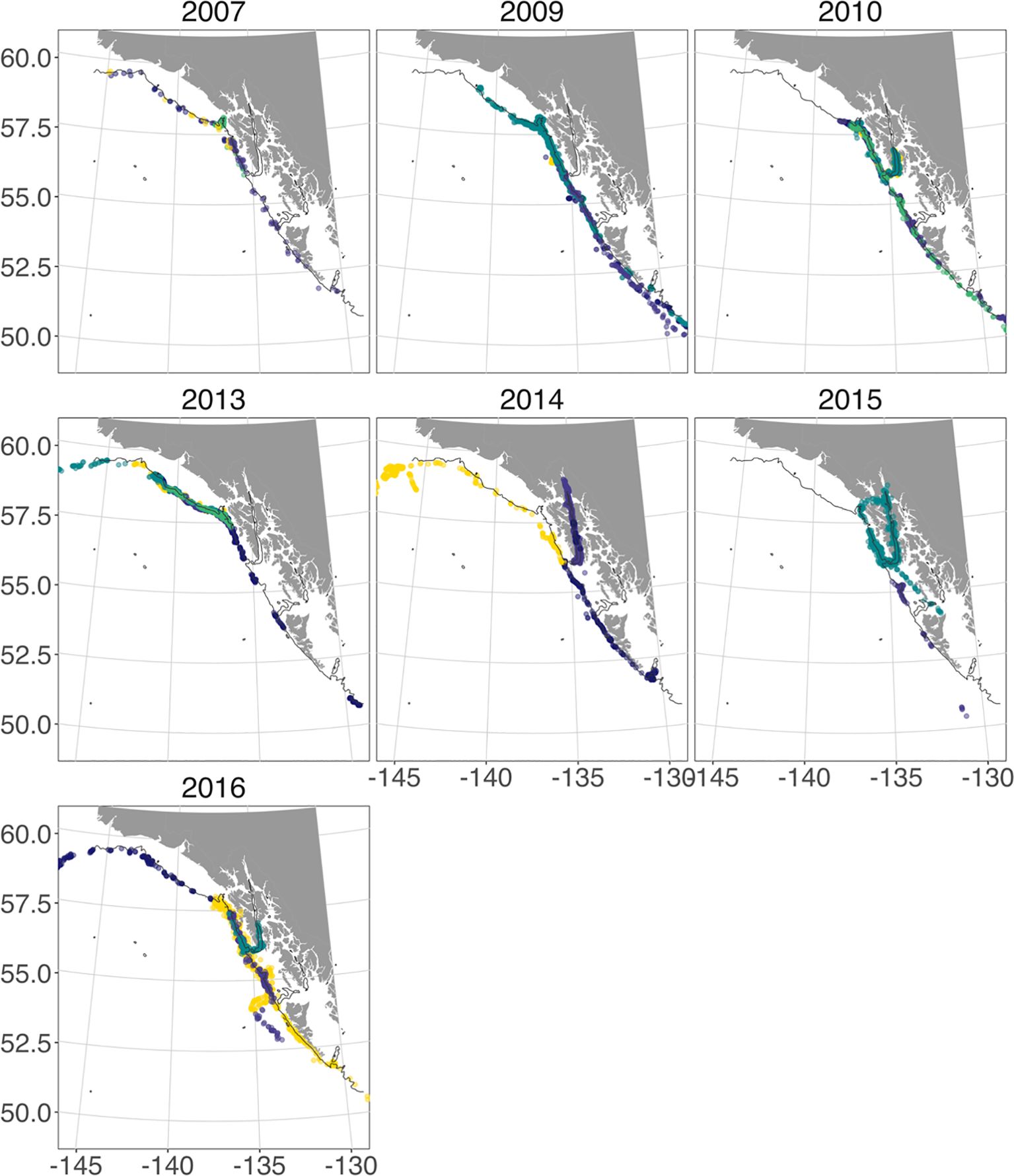
Figure 2. Satellite tag position estimates from filtered Argos data for all tags by year showing movement within the eastern Gulf of Alaska. The thin black line represents the bathymetric contour line at 350m depth. Different colors each year denote individual tagged whales. Full tag tracks are available in Supplementary Material S3.

3.2 Objective 1: general patterns in sperm whale movement and diving behavior

3.2.1 Regional movement

Of the 29 whale tracks analyzed, nearly 1/3 (n=10) generally moved northwest, out of the study area and towards the Central GOA (Figure 2). The remaining whales either stayed in the study area (n=5) or moved south (n=14) while the tag was on the whale. Nine of the tagged whales moved south past the southern tip of Haida Gwaii Island, British Columbia (~52°N Latitude) into Queen Charlotte Sound waters before the tags stopped transmitting. Of the whales that moved south and out of the GOA (~52°N Latitude), none turned around and moved northward again at any point while tags were transmitting. However, three tagged animals turned around and spent time off Haida Gwaii between 52°N and 54°N Latitude. Tagged whales left the GOA heading south during a variety of summer, fall, and winter months, with two whales heading south in June, one in July, one in August, one in September, three in October, and one in January. Five tags stayed on whales that moved south of Washington state. These animals all moved to points offshore of California or Mexico before the tags stopped transmitting (Supplementary Material S3).

3.2.2 Horizontal movement

The minimum daily rate of horizontal movement across all tagged whales had a median of 1.7 km/hr (38.6 km/day) but was highly variable, ranging from 0.04-7.79 km/hr (mean = 2.2 ± 1.8 km/hr). This result was independent of the number of locations used per day in the calculation. For the tagged whale positions that were within the GOA (north of 52°N Latitude), the median minimum daily rate of horizontal movement was 1.4 km/hr (33 km/day), similar to the overall median. However, when considering only tagged whales that moved out of the GOA, the median minimum daily rate of horizontal movement increased to 5.5 km/hr (123 km/day) after whales left the GOA, indicating whales had a tendency to speed up or move in a more linear fashion after leaving the GOA (Figure 3).

Figure 3

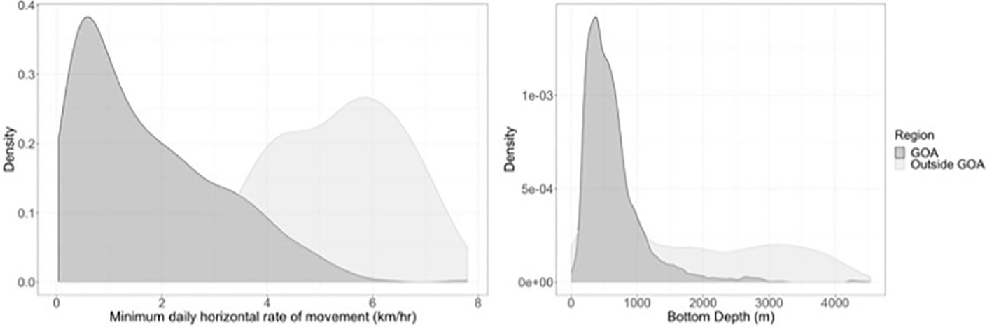
Figure 3. Density plot showing minimum rates of horizontal movement in the GOA versus outside the GOA. Whales have higher rates of movement after they leave the GOA.

Seafloor depth under tagged whale positions averaged 768 m (± 716 m), with 75% of all positions being classified as over the continental slope, 18% over the continental shelf, and 7% over the deep ocean basin. Average seafloor depth at interpolated sperm whale position estimates within the GOA (651 m) was shallower than outside the GOA (1806 m) (Figure 3).

3.2.3 Use of inside waters

In 2010, two whales (SWsat13 & SWsat15) that were tagged in the northern part of the study area moved south along the continental shelf edge after tags were attached, and then turned into inside waters of Chatham Strait in Southeast Alaska (Supplementary Material S3). This occurred in late August, while the state-managed sablefish fishery was taking place in Chatham Strait. These tracks represent a continued association of two specific male sperm whales over a period of 43 days and these same two individuals were again sighted together near a fishing vessel in Chatham Strait in 2014 and in 2015. In 2014 SEASWAP focused some tagging efforts in Chatham Strait to specifically target animals that were using inside waters while the fishery was taking place. Two whales were tagged in Chatham Strait in 2014, one in 2015, and one in 2016 (Supplementary Material S3). Over all the years SEASWAP has documented sperm whales in Chatham Strait (2010, 2014, 2015, and 2016), only three different individuals have been identified using photo-identification. These individuals are GOA-023 (SWsat13), GOA-091 (SWsat15, SWsat27, SWsat28, and SWsat33), and GOA-086 (SWsat26). In 2015, one of these tagged whales, GOA-091 (SWsat28) circumnavigated Baranof and Chichagof Islands, moving through shallower waters in Icy Strait that are not typical sperm whale habitat. Another of these whales, GOA-086 (SWsat26), traveled northward into Lynn Canal, moving outside of the commercial sablefish fishery area while the fishery was still taking place. Figures of these tag tracks are available in the Supplementary Material (Supplementary Material S3, Supplementary Figure S3.2).

3.2.4 Dive behavior

Fourteen tags provided diving information, resulting in 7,573 total dives (from Behavior Log dive data) to examine overall dive behavior. Dive durations and maximum dive depths appeared to be similar among different individuals (Figure 4), with the mean maximum dive depth ranging from 350 m to 507 m across the fourteen tag records (overall average = 396 m ± 116 m) and the mean dive duration ranging from 29min to 38min (overall average = 32 min ± 9 min) (Table 2). The maximum recorded dive depth was a 1848 m dive by SWsat13 in October of 2010. The longest dive recorded was a 112-minute dive in May 2013 (SWsat20). GOA-091, the individual tagged four times, had dive data recorded for three of its tags (SWsat15, SWsat27, and SWsat33) with a total of 1,474 dives. The mean dive depths of these three deployments varied considerably, at 507 m (± 222 m), 406 m (± 186 m), and 369 m (± 160 m) respectively.

Figure 4

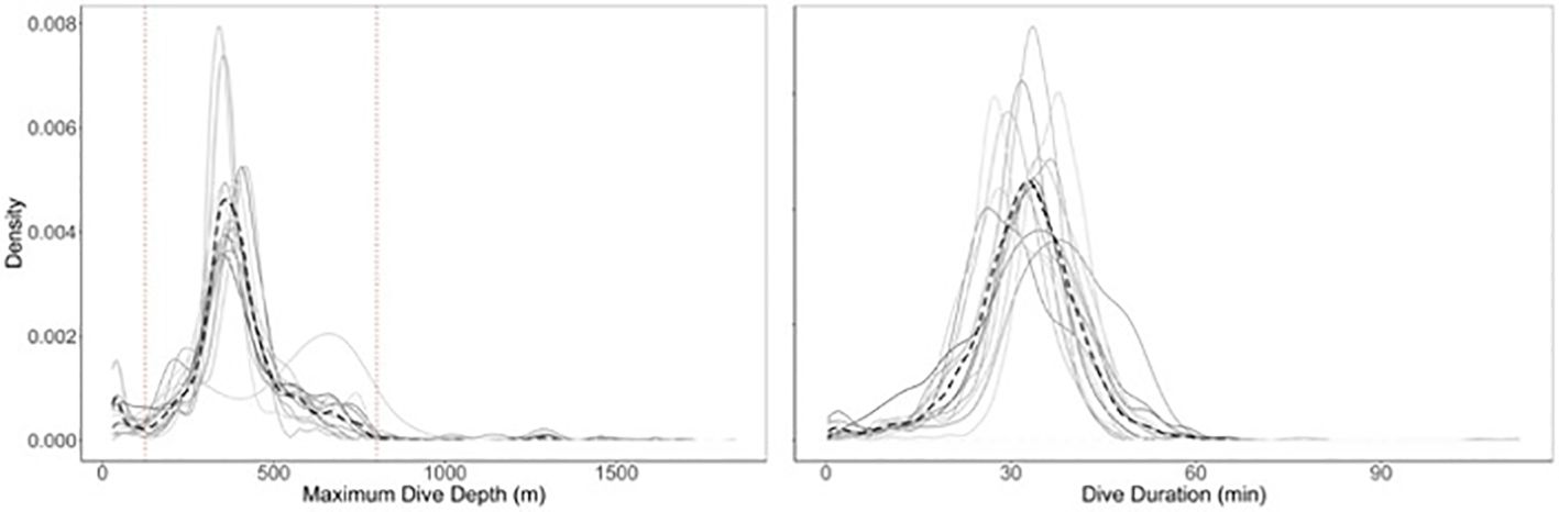
Figure 4. Density plots of maximum dive depth and dive duration for 14 tags with dive data. Dashed black line represents the average of all tags. Dotted vertical lines in left-hand panel are at 125m and 800m, reflecting the cutoff depths for intermediate dives.

Table 2

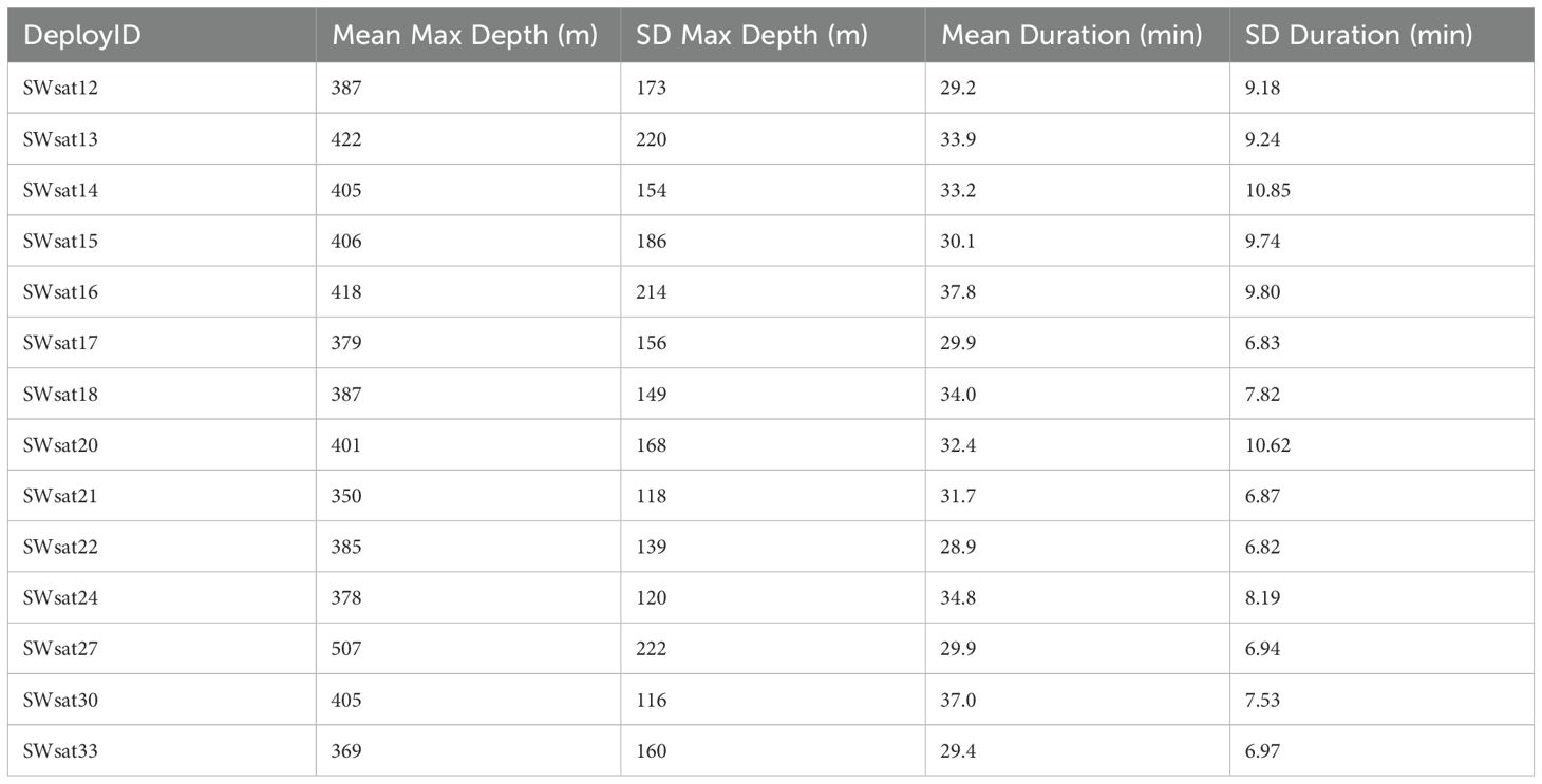
Table 2. Summary statistics of dive information for each tag that transmitted diving behavior, showing mean and standard deviation (SD) for the maximum depth and duration of dives.

A majority of dives for all tag records combined were square-shaped (71%), followed by U-shaped dives (23%), and V-shaped dives (6%) (Table 3). This pattern was fairly consistent across all individual tags that recorded diving information, though there was some variability in the proportion of each dive shape an animal exhibited (Supplementary Material S4). Linear mixed effects models (LME) showed maximum dive depth and duration both varied significantly with respect to all dive shapes (Square, U-, and V-shaped), with individual ID as a random effect. For fixed effects in the dive duration LME, the intercept (representing the mean dive duration for the square dives) was estimated at 33.98 minutes (SE = 0.74, t = 45.62, p < 0.001). The shape U was associated with a significant reduction in dive duration by 5.51 minutes (SE = 0.23, t = -23.79, p < 0.001), and shape V was associated with a significant reduction in dive duration by 6.22 minutes (SE = 0.43, t = -14.55, p < 0.001). The correlations between the fixed effects were low, with -0.080 between the intercept and Shape U, and -0.047 between the intercept and Shape V, indicating minimal multicollinearity. For fixed effects in the dive depth LME, the intercept (representing the mean dive duration for the square dives) was estimated at 399 m (SE = 9.45, t = 42.23, p < 0.001). The shape U was associated with a significant increase in dive depth by 24.4 m (SE = 4.53, t = 5.37, p < 0.001), and shape V was associated with a significant reduction in dive depth by 97.6 m (SE = 8.37, t = -11.7, p < 0.001). The correlations between the fixed effects were low, with -0.123 between the intercept and Shape U, and -0.072 between the intercept and Shape V, indicating minimal multicollinearity. Finally, a LME of bottom depth with respect to dive shape indicated that square and U-shaped dives varied significantly with bottom depth. Square shaped dives were estimated to be over 566 m bottom depth (SE=25.5, t=15.95, p<0.001), while U-shaped dives were over significantly deeper bottom depths by 35.4 m (SE=12.65, t=1.39, p<0.001). The correlations between the fixed effects were low, with -0.143 between square and U-shape, and -0.078 between square and V-shape, indicating minimal multicollinearity.

Table 3

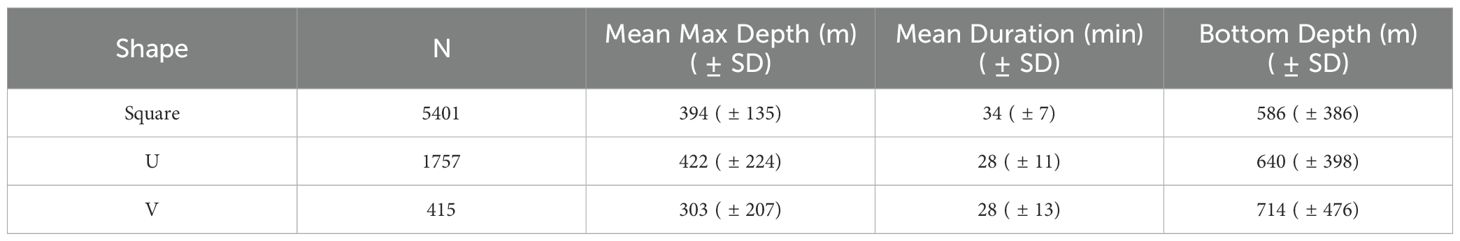
Table 3. Summary of dive shape with respect to maximum dive depth, duration, and associated seafloor depth.

Of the individual dives recorded in the GOA, 75% were square-shaped, 19% were U-shaped, and 6% were V-shaped. Meanwhile, of the individual dives recorded outside of the GOA, 62% were square-shaped, 35% were U-shaped, and 3% were V-shaped. A Pearson’s Chi-squared test revealed no significant differences in the dive shape composition between the GOA and areas outside the GOA (X² = 4.76, df=2, p=0.93).

3.3 Objective 2: characterize foraging and transiting behavior to identify foraging hotspots of sperm whales in the GOA

Raw position data for the period of time the tags transmitted daily (8,729 positions) were analyzed with state-space models to interpolate an estimated position every three hours, resulting in a total of 5,817 position estimates. Diagnostics indicated models converged well; within-chain sample autocorrelation was low and Brooks-Gelman-Rubin scale reduction factors were <1.1 for all tags.

To characterize foraging and transiting behavior the full SSM output data was further filtered to include only data points where behavioral states had a high degree of certainty, 1<b<1.25 and 1.75<b<2 (Jonsen et al., 2005, 2007). This resulted in a total of 4,505 positions with an estimated behavioral state. Overall, behavior was primarily classified as foraging (74% of positions) versus transiting (26% of positions). Within the GOA, models predicted primarily foraging behavior, with 82% of interpolated positions classified as foraging versus 18% transiting. Foraging was spread out along the entire slope region within the core study area with a lack of particular hotspots, and binomial models showing the probability of foraging showed similar trends in that foraging was relatively high throughout the region without clear hotspots (Figure 5). Outside the GOA, whale behavior was primarily classified as transiting, with 74% of interpolated positions being classified as transiting versus 26% foraging. Square-shaped dives made up 78% of transiting dives and 74% of ARS (foraging) dives. A Pearson’s Chi-squared test revealed no significant differences in dive shape composition between ARS and transiting dives (X² = 5.82, df=2, p=0.06).

Figure 5

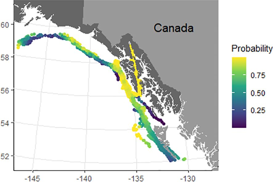
Figure 5. Smoothed probability of foraging based on predicted foraging behaviors for 29 satellite tag deployments.

Seafloor depth at modeled 3-hourly tag positions averaged 828 m (± 789 m; median=570 m), with 18% of all positions being classified as over the continental shelf, 73% over the continental slope, and 9% over the deep ocean basin. A t-test revealed a significant difference in bottom depth between ARS and transiting locations (t=28.13, df=1650, p<2.2e-16), with mean bottom depth (+/- sd) in transiting locations being 1464 m (+/- 1169 m) and mean bottom depth over foraging locations being 603 m (+/- 407 m). The slope of the bathymetry in 1 nm grid cells under tag positions within the study area averaged 5.7 degrees (± 4.9 degrees). A t-test revealed significant differences in slope between ARS and transiting locations (t=10.29, df=726, p<2.2e-16) with mean slope (+/- sd) in foraging locations being more steep (8.0 +/- 6.3 degrees) than in transiting locations (5.3 +/- 4.5 degrees).

3.4 Objective 3: identify environmental drivers of diving behavior

Full model selection output for dive depth and dive duration models is available in Table 4. The best model for intermediate (125 – 800 m) dive depths was the full model, including light level, lunar cycle, seafloor depth, slope, CPUE, and individual tag ID (Table 5). Variance inflation factors were below 2 for all variables, indicating multicollinearity does not pose an issue for the stability and interpretability of the model (VIF values were Light=1.01; lunar = 1.07; Bottom Depth = 1.06; CPUE = 1.09; slope = 1.12). The model explained 33% of the deviance in maximum dive depth, with most of the deviance explained by seafloor depth, followed by light level, CPUE, lunar cycle, individual whale variability, and slope (Table 5). Seafloor depth was most strongly related to maximum dive depth, explaining 22 to 24% of the deviance in the model, followed by CPUE (6-10% of the deviance) and individual whale ID (1-6% of deviance) (Table 5). Dives tended to be slightly deeper during the day and at night, as well as during quarter moons, when tidal currents are weakest (Figure 6). Dive depth increased with seafloor depth up to about 800 m, in part reflecting the constraint that dive depths cannot exceed bottom depths. Dive depth decreased over deeper water, although variability was high. Average dive depth decreased slightly as the slope of the seafloor increased. Sablefish CPUE in the fishery and dive depth were inversely related, with dive depth decreasing in areas of higher CPUE (Figure 6).

Table 4

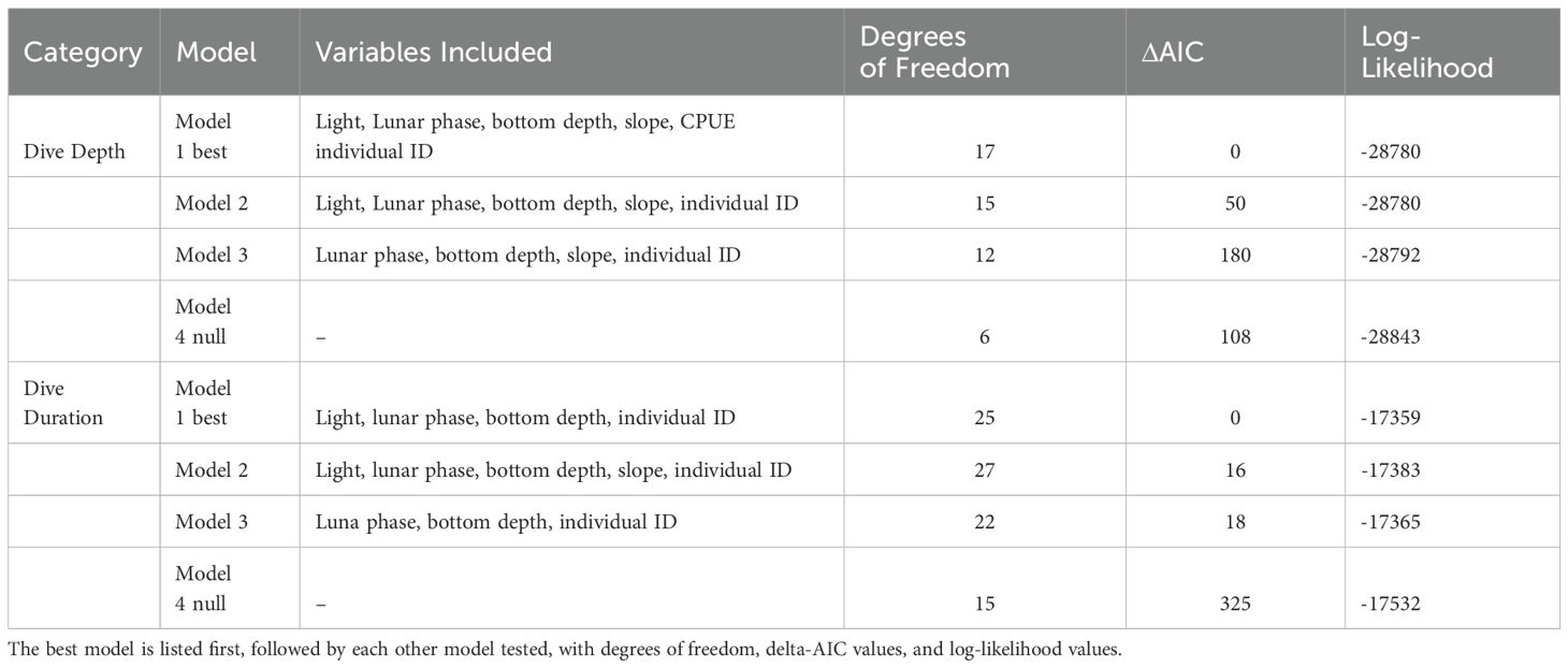
Table 4. Model selection table showing dive depth models and dive duration models.

Table 5

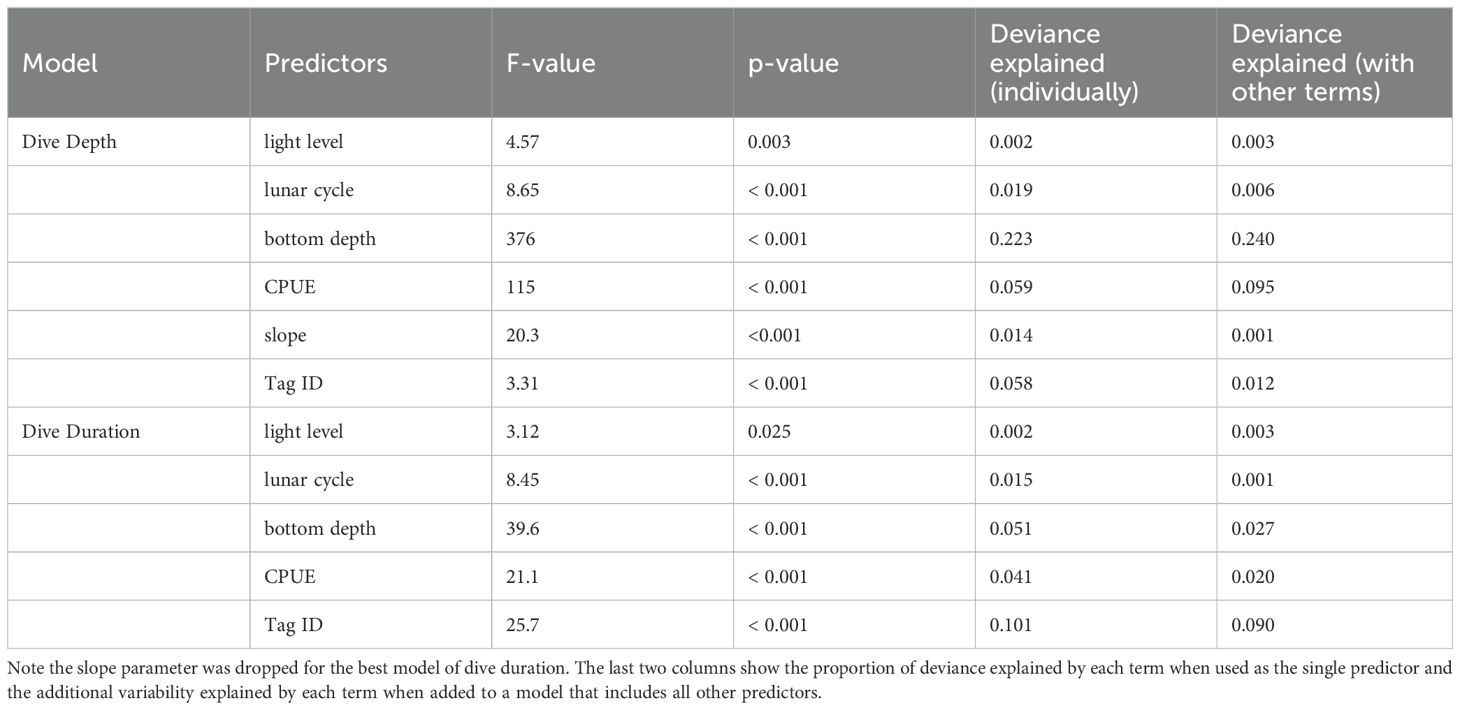
Table 5. Summary output of dive depth and duration models.

Figure 6

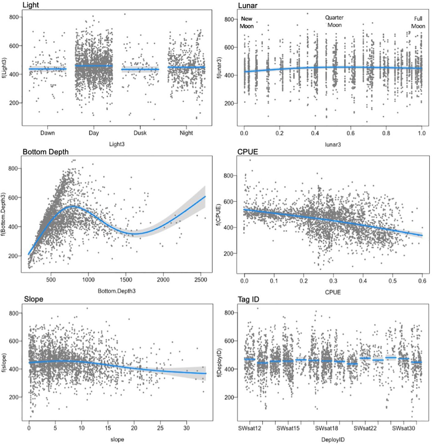
Figure 6. Model output of environmental covariates that influence dive depth, showing the smooth effect of each variable on dive depth (y-axis), conditional upon the other terms in the model at their median values. The line represents the prediction line with grey confidence band, and points represent partial residuals.

The best model for dive duration included all predictors except slope (Table 5) and explained 18% of the deviance. Variance inflation factors were below 2 for all variables, indicating multicollinearity does not pose an issue for the stability and interpretability of the model (VIF values were Light=1.01; lunar = 1.05; Bottom Depth = 1.05; CPUE = 1.03). Most of the explained variability was attributed to differences in mean dive duration among individual whales (‘DeployID’), which accounted for 10% of the overall deviance. Seafloor depth explained 3-5% of the deviance and sablefish CPUE explained 2-4% (Table 5). Dive duration varied little among light levels but showed a pattern of slightly longer dives during crescent to quarter moons (Figure 7). Dive duration increased as seafloor depth increased, but the estimated relationship leveled off above approximately 1,000 m. Durations decreased as sablefish CPUE increased, with the shortest dives at a CPUE of approximately 0.3 kg per hook, and then dive durations increased again as CPUE kept increasing. Individual variability was significant, where a few individuals had longer dives on average (SWsat16 and SWsat27 (Figure 7)).

Figure 7

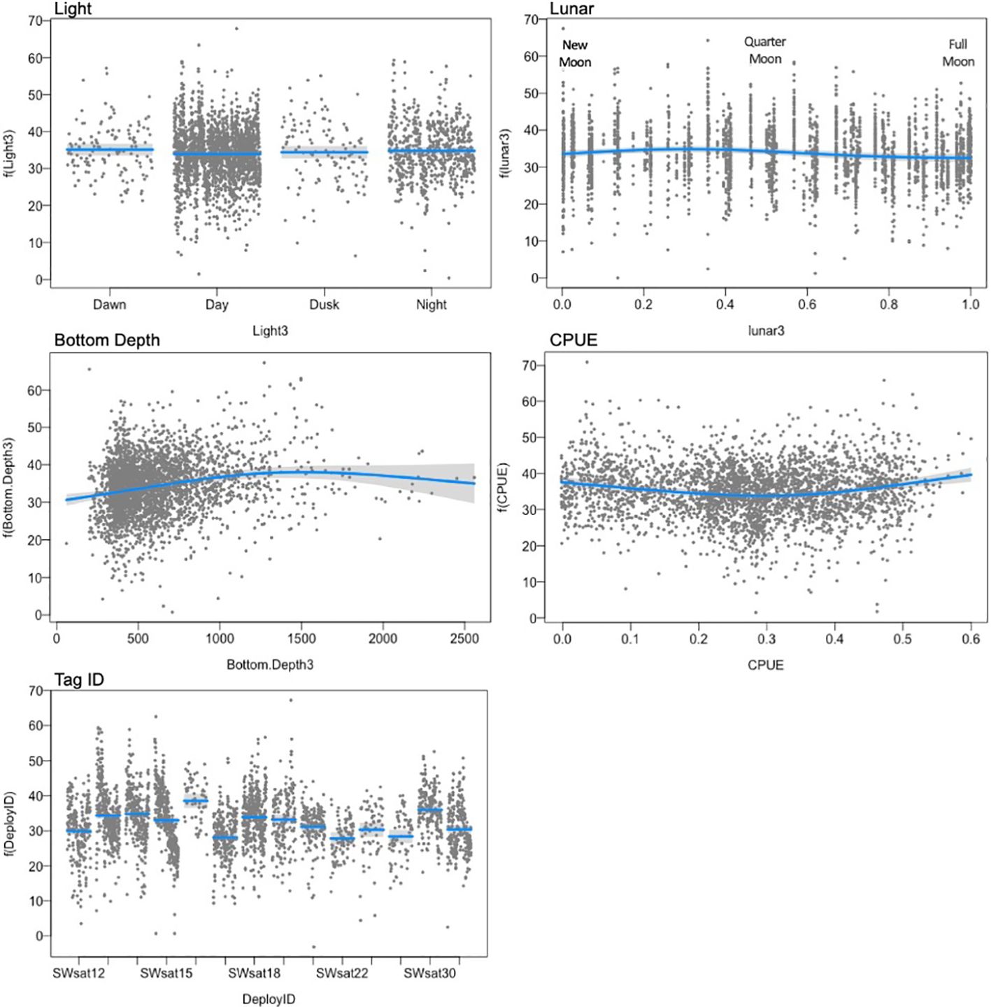
Figure 7. Environmental covariates from the best model for dive duration of sperm whales, showing the smooth effect of each variable on dive duration (y-axis), conditional upon the other terms in the model at their median values. The line represents the prediction line with grey confidence band, and points represent partial residuals.

4 Discussion

4.1 General movement patterns

We found that tagged whales in our study made broad movements along the continental slope, with little movement over the deep ocean basin. The timing of sperm whale migrations, specifically movement of males, is largely unknown (Whitehead, 2003). One-third of whales tagged in the eastern GOA moved north towards the central GOA, while just over half of the whales moved south after tags were deployed and before they stopped transmitting. Nine tagged whales left the GOA heading south and did not turn around after moving south of 50°N Latitude while the tags were transmitting. Interestingly, these whales left Alaska during a variety of months and seasons (summer, fall, and winter). We note, however, that this data set consists of whales tagged from May to September, which biases our information on timing of migrations due to an average tag deployment duration of 45 days. However, even with the limited seasonal tag deployments, our data suggests that male sperm whales in the GOA do not necessarily exhibit predictable seasonal migrations.

Tagged whales that left Alaskan waters headed south toward warmer equatorial waters off Mexico, and some went into the Sea of Cortez where breeding female and juvenile groups are known to congregate and mature males have been seen (Jaquet and Gendron, 2002, 2003, 2009; Ruiz-Cooley et al., 2004; Davis et al., 2007). Behavioral state of tagged whales switched from primarily foraging in the GOA waters to primarily transiting when they left GOA waters heading south. Whales also sped up after leaving the GOA, emphasizing this change in behavior, consistent with findings from Straley et al. (2014). These findings suggest the GOA is an important foraging area for these individuals, in that they did not appear to spend time foraging in other regions during their migrations and while tags were transmitting.

The use of inside waters of Chatham Strait by multiple tagged whales, representing three individuals, has not been previously documented in this region. Chatham Strait is a deep fjord with depths exceeding 700 m, where sablefish inhabit, and which are well within the depth range sperm whales inhabit in their offshore habitat. The State of Alaska manages a limited entry sablefish fishery in Chatham Strait that is open from mid-August to mid-November each year. The two whales (SWsat13 and SWsat15) tagged in early August 2010 offshore who moved south together and entered inside waters of Chatham Strait, were also seen depredating the same vessel in 2014, and present an interesting association not previously documented in this region. Though male sperm whales are thought not to form associations (Lettevall et al., 2002; Mizroch and Rice, 2013), we believe that this may show a unique example of a long-term association between two individuals. Alternatively, it could be that these two individuals were simply exploiting the same opportunity and were coincidentally sighted together depredating across multiple years. Genetic sampling of these individuals could reveal more information about their relatedness.

The maximum dive depth and dive duration of sperm whales in the GOA (396 m ± 116 m and 32 min ± 9 min) is within the observed range of dive depths and durations documented for both males and females in the Gulf of California (Davis et al., 2007; Gallo-Reynoso et al., 2009; Irvine et al., 2017), and on the shallow end of recorded dives from male sperm whales in other high latitude regions such as Norway (mean 492 ± 593 m) and Kaikoura, New Zealand (mean 924 m) (Teloni et al., 2008; Guerra et al., 2017) (Table 6). Given the topography of all three regions is similarly characterized by steep and productive slopes, the sperm whales in the GOA may be diving slightly shallower on average due to location of prey they are targeting, the depredation activity leading to shallower dives, or the influence of fishing vessels being in shallower water and bringing whales into slightly shallower habitat. Sablefish longline sets range from 150-900 m with a majority being 400-600 m. The single individual (GOA-091) tagged four times across six years (with three years containing dive behavior information) exhibited the shallowest average (± SD) maximum dive depths (396 m ± 160 m) of all tagged whales, and also the deepest maximum dive depths (507 m ± 223 m) of all tagged whales. This suggests that variability in maximum dive depth may not relate to individual preference or physiological constraints but instead may be more related to other factors (e.g. the location where individuals are tagged, where they spend their time during tag deployment, etc.).

Table 6

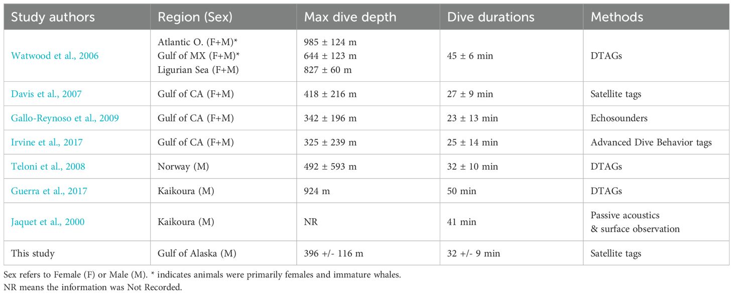
Table 6. Other sperm whale studies (both tagging and acoustic methods) including dive depth and/or durations around the world.

Dives consisted mostly of square-shaped dives across all tags (Table 3). Interestingly, V-shaped dives and U-shaped dives had the same average duration (28 min), but V-shaped dives were on average over 100 m shallower than U-shaped dives (Table 3). This indicates they are likely used for different purposes than square and U-shaped dives, with whales spending very little to no time in the bottom phase of V-shaped dives (<20% total dive time, Supplementary Material S4). Because V-shaped dives had the same duration, but their maximum depth was much shallower, we contend that these dives likely serve a transiting or searching purpose, but likely do not indicate successful foraging. Irvine et al. (2017) found V-shaped dives to have a similar depth as in our study (median maximum depth of 290 m) and found that the depth was highly correlated to the depth of the preceding foraging dive, indicating they were likely intended for searching. Square-shaped and U-shaped dives both likely represent foraging dives and given their similarities could be grouped. Other studies exploring dive shape use different categories and classifications of dive type, making it difficult to compare across studies (Amano and Yoshioka, 2003; Fais et al., 2015; Irvine et al., 2017). In the future, using dive shapes, durations, and maximum depths in behavioral modeling, when available, could help determine behavioral states of this species. In addition, high resolution accelerometry tags allow for 3D modelling of dives and estimation of when and where prey capture attempts occurred (Mathias et al., 2012).

Much of the dive behavior for male sperm whales in high latitudes has been studied off the coast of Norway and New Zealand, using short-duration archival tags attached to whales for a number of hours, rather than days, using suction cups. Overall, these studies indicate that male sperm whales in high latitudes forage in both bathypelagic and mesopelagic zones, they often switch between the two zones during a single day, and preference for foraging zones in the water column is likely a reflection of varying productivity and prey availability (Teloni et al., 2008; Fais et al., 2015, 2016; Guerra et al., 2017; Isojunno and Miller, 2018). Our results show whales dive to a variety of depths and occasionally switch between discrete depths (Supplementary Material Figure S4.5), consistent with these other studies.

4.2 Dive behavior modeling

Whales dove deeper and longer during the daytime and during quarter moon lunar cycles. Dives became shallower in areas of increasing sablefish CPUE, which could indicate depredation behavior and feeding off of longline gear as it is being retrieved. Maximum dive depth increased as seafloor depth increased, up to approximately 800 m seafloor depth, at which point dives became shallower again. Individual variability in dive depth and particularly in dive duration was high. Maximum dive depth and dive duration were most strongly related to seafloor depth (22% and 5% of deviance explained, respectively), individual Tag ID (6% and 10% of deviance explained), and CPUE of the sablefish fishery (6% and 4% of deviance explained). Other significant predictors to both models included light levels and lunar cycle, though these variables explained less of the deviance (Table 5). Slope was not strongly associated with dive depth and was not included in the best model of dive duration, suggesting the steepness of the seafloor is of little to no importance in sperm whale diving behavior.

When modeling sablefish CPUE (a measure of sablefish abundance), we found sablefish CPUE increased with increasing seafloor depths before decreasing below ~1100 m (Supplementary Material S2), so dive depth would be expected to increase with sablefish CPUE if whales were naturally foraging for sablefish. However, models of dive depth and duration suggested shorter and shallower dives with increasing CPUE (Figures 6, 7), which may indicate depredation behavior, where whales do not need to dive as deep or as long when feeding from longline gear. Whales may be attracted to the high CPUE areas less by high sablefish abundance and more by the easy targets presented by fishing boats.

Lunar cycle and time of day (dawn, day, dusk, night) were less influential but still significant predictors of maximum dive depth and duration. These variables tend to be important to diel movements of prey in the ocean in general, where the deep scattering layer (DSL) undergoes diel vertical migrations (DVM) and rises from deeper water to more mesopelagic and subsurface waters at night (Eyring et al., 1948; Johnson, 1948). There is little consensus on diel behavior of diving sperm whales in the literature (Irvine et al., 2017; Stanistreet et al., 2018). Guerra et al. (2017) found some evidence of different dive depths targeted between day and night, measured using acoustic buzzes (foraging creaks). For this study, we found that sperm whale dives in the GOA were slightly deeper and shorter on average during the daytime than at dawn, dusk, or night, indicating potential responses to movement of prey. The mesopelagic zone in high latitudes has been found to extend between 100-400 m during the day, rising above 200 m at night, and also exhibits seasonal fluctuations (Cooney, 1989; O’Driscoll et al., 2009; Klevjer et al., 2016). In the GOA, there is evidence of diel vertical migrations for many sperm whale prey species, including sablefish, rockfish, and spiny dogfish (Hunsicker et al., 2010; Carlson et al., 2014; Tribuzio et al., 2017; Sigler and Echave, 2019). For sablefish in particular, however, reverse DVM is also shown in this region, with fish moving to shallower waters during the day and descending at night (Sigler and Echave, 2019). Our results likely reflect changes in sperm whale foraging on their primary groundfish and squid prey as they respond to changes in light levels. The fact that diel cycles were less influential to the model may simply be a result of the restricted summer sampling season when there is very little darkness, as well as the lack of large vertical excursions between day and night for some of their prey.

Lunar cycles can influence prey movement as well because full moon phases are associated with more light than new moons, affecting the degree of DVM. In addition, lunar cycles affect tidal cycles and oceanic currents. A recent study on the diving behavior of pilot whales off the Hawaiian islands revealed that during full moon phases, pilot whales performed dives that were deeper, longer, and farther from shore than during new moons, potentially reflecting vertical movement of their primarily squid prey (Owen et al., 2019). For our study, dives did not appear to reflect differences between full moon or new moon phases. This could be due to a variety of factors including differences between species, habitat, and/or differences in prey preferences. Heavy cloud cover and storm systems obscuring illumination from lunar cycles in the GOA could reduce the influence of lunar phase on sperm whale prey, and thus the diving behavior of sperm whales. Research on zooplankton has indicated that while it likely cannot explain all of the variability in responses to lunar cycles, cloud cover and changes in light can explain some variability in zooplankton responses to lunar cycles (Klevjer et al., 2016). Sperm whale prey differs from that of pilot whales in that they consume a larger proportion of groundfish than squid in our study area (Wild et al., 2020), which may not respond to lunar illumination in the same manner as squid, though research on lunar cycles with respect to groundfish movement in this region is lacking.

4.3 Additional considerations

The behavioral state space models we used were adequate for broad comparisons of foraging and transiting behavior within and outside the GOA but may not be ideal for identifying more fine-scale foraging hotspots of sperm whales. The main issue with these models was that there was extreme temporal autocorrelation because of the long periods of either foraging or transiting. For this study, we were interested in identifying foraging hotspots within the GOA region, where switches between transiting and foraging states could be happening at smaller time scales than our data resolution could achieve, or at larger time scales than we can resolve in this analysis. In addition, sperm whale prey of groundfish and squid may not be found in dense aggregations, thus their switches between foraging and transiting may be more subtle, and difficult for these models to detect. Finally, sperm whales in this region may also be more graze-as-you-go foragers, constantly foraging and searching for prey on dives, even while transiting or migrating. This may be evidenced by the fact that even when they left the GOA, tagged whales continued to perform deep dives. Animals focused solely on transiting may choose not to expend the energy to make deep dives.

4.4 Conclusions

This study explored satellite tag data from a high latitude male sperm whale population, including behavioral state estimation and dive behavior analysis over longer time periods. The findings from this work increases our knowledge of sperm whale movement and diving behavior in the North Pacific and has important management implications. Our results confirm that the GOA is an important foraging ground for these male sperm whales, and tagged whales spent a considerable portion of the year in the GOA, which is critical when considering management and recovery plans for this endangered species. Timing of migrations to and from Alaskan waters is also important from a management perspective, especially considering these sperm whales interact with an important commercial fishery. While migratory analysis was not a focus of this study, we found no predictable timing of migration for the whales tagged in this study, though a majority of the tagged whales that left the GOA heading south did so in the late summer and fall months which is during the current longline fishing season from mid-March to mid-November. Increasing the sample size of tag records, focusing analysis on migration, and targeting tagging efforts in the winter and spring may shed more light on the timing of migrations and when whales arrive and depart Alaskan waters.

Tagged whales dove almost continuously, often making deep dives, where they were likely feeding on groundfish prey, including sablefish. The proportion of sablefish in sperm whale diets has increased over recent decades (Wild et al., 2020), during a time when sablefish biomass has generally decreased (Hanselman et al., 2018). Therefore, it is important for stock assessments to consider this additional source of sablefish mortality (both through depredation and potentially increased natural foraging) when assessing regional biomass of this commercially important species. In addition to sperm whale depredation as an additional source of mortality, killer whales also depredate sablefish from fishing gear in the GOA (Yano and Dahlheim, 1995), which has a greater impact on the annual stock assessment, as well as on the fleet, than sperm whale depredation (Hanselman et al., 2018). Thus, the effects of removals from sperm whales and killer whales combined likely have a significant impact on the resource and incorporating all sources of mortality into assessments is important to determining sustainable harvest levels.

More broadly, our results identify a high potential for further conflict, as depredation may be a new and growing behavior facilitated by an overlap between natural foraging areas and the sablefish fishery in the GOA over the continental slope region. As sperm whale populations are assumed to be increasing world-wide with the cessation of commercial whaling removing the main source of mortality to the species, better understanding of their movement patterns in their GOA foraging grounds will be crucial to effectively protect fisheries resources and whale populations.

Data availability statement

The datasets presented in this study can be found in online repositories. The names of the repository/repositories and accession number(s) can be found here: GitHub Repository: https://github.com/LaurenWild/UAF_PhD_Ch3.

Ethics statement

The animal study was approved by University of Alaska IACUC Protocols #906340-1 and #157884-14. Additionally this work was conducted under NMFS scientific research permit numbers 14122 and 18529. The study was conducted in accordance with the local legislation and institutional requirements.

Author contributions

LW: Conceptualization, Formal analysis, Funding acquisition, Investigation, Methodology, Software, Writing – original draft, Writing – review & editing. FM: Conceptualization, Formal analysis, Investigation, Methodology, Resources, Software, Supervision, Validation, Writing – original draft, Writing – review & editing. JS: Conceptualization, Funding acquisition, Investigation, Project administration, Resources, Supervision, Validation, Visualization, Writing – original draft, Writing – review & editing. RA: Conceptualization, Formal analysis, Investigation, Methodology, Resources, Writing – original draft.

Funding

The author(s) declare financial support was received for the research, authorship, and/or publication of this article. Tagging fieldwork was performed with funding from a variety of sources from 2007 to 2016: the North Pacific Research Board (Projects 0626 Sperm Whale Depredation, 0918 Sperm whale depredation, and 1217 Countermeasures to reduce whale depredation in Alaskan longline fisheries), Oil and Gas Producers Association, NOAA Fisheries Auke Bay Lab (vessel time on F/V Northwest Explorer), NOAA’s Saltonstall-Kennedy grant program (Award #NA15NMF4270271), and the Central Bering Sea Fishermen’s Association. Funding for analysis and manuscript prep came from the Biomedical Learning and Student Training (BLaST) program at the University of Alaska Fairbanks. BLaST is supported by the NIH Common Fund, through the Office of Strategic Coordination, Office of the NIH Director with the linked awards: TL4GM118992, RL5GM118990, UL1GM118991.

Acknowledgments

Special thank you to SEASWAP partners Linda Behnken and Dan Falvey of the Alaska Longline Fishermen’s Association, Dr. Aaron Thode, Victoria O’Connell Curran, and Jennifer Cedarleaf for project support and administration in this collaborative work. Extensive feedback on analysis and manuscript was provided by Mike Sigler and Bree Witteveen. Additional tagging work from John Calambokidis, Dr. Greg Schorr, and Dr. Erin Falcone of Cascadia Research Collective and Marine Ecology & Telemetry Research. Sablefish catch data courtesy of Dana Hanselman of NOAA Fisheries Alaska Fisheries Science Center (AFSC) Ted Stevens Marine Research Institute (TSMRI).

Conflict of interest

The authors declare that the research was conducted in the absence of any commercial or financial relationships that could be construed as a potential conflict of interest.

Publisher’s note

All claims expressed in this article are solely those of the authors and do not necessarily represent those of their affiliated organizations, or those of the publisher, the editors and the reviewers. Any product that may be evaluated in this article, or claim that may be made by its manufacturer, is not guaranteed or endorsed by the publisher.

Supplementary material

The Supplementary Material for this article can be found online at: https://www.frontiersin.org/articles/10.3389/fmars.2024.1394687/full#supplementary-material

References

Aarts G., MacKenzie M., McConnell B., Fedak M., Matthiopoulos J. (2008). Estimating space-use and habitat preference from wildlife telemetry data. Ecography 31, 140–160. doi: 10.1111/j.2007.0906-7590.05236.x