 Yulin Wang
 Jingui Liu
 Lingling Xie
 Tianyu Zhang
 Lei Wang2
94% of researchers rate our articles as excellent or good
Learn more about the work of our research integrity team to safeguard the quality of each article we publish.
Find out more
ORIGINAL RESEARCH article
Front. Mar. Sci., 18 July 2024
Sec. Physical Oceanography
Volume 11 - 2024 | https://doi.org/10.3389/fmars.2024.1391087
The combination of typhoon-induced storm surges and astronomical tides can result in extreme seawater levels and disastrous effects on coastal socioeconomic systems. The construction of an appropriate wind field has consistently been a challenge in storm tide forecasting and disaster warning. In this study, we optimized a nonlinear regression formula based on the C15 model to determine the maximum wind radius. The simulation based on the improvement showed good accuracy for storm tides during super typhoon Mangkhut (WP262018), Saola (WP092023), and severe typhoon Hato (WP152017). The correlation coefficients were in the 0.94–0.98 range, and the peak bias was less than 5cm. The trough errors were significantly reduced compared to other wind fields. Owing to the importance and lack of the maximum wind radius (Rmax), we attempted to predict Rmax using an LSTM (Long Short-Term Memory) neural network for forecasting storm tides during strong typhoons. Constrained LSTM showed good performance in hours 6–48, and effectively enhanced the forecasting capability of storm tides during strong typhoons. The workflows and methods used herein have broad applications in improving the forecasting accuracy of strong typhoon-induced storm tides.
Strong winds and sudden changes in atmospheric pressure associated with the passage of a tropical cyclone (TC) cause localised oscillation or nonperiodic abnormal rise (or decrease) of the sea surface, referred to as a storm surge (Needham et al., 2015). Storm surges coinciding with astronomical tides, especially astronomical high tides, often result in severe coastal flooding disasters (Muis et al., 2016). As more than 600 million people worldwide reside in coastal areas (McGranahan et al., 2007), storm tides can cause severe disasters to society (Hinkel et al., 2014). The threat of storm tides has recently intensified owing to anthropogenic disturbances, global climate change, and the increased vulnerability of coastal lands. Therefore, the accurate and timely prediction of typhoon-induced storm tides has become a global concern for the development of early warning systems for marine disasters. Increasing the forecasting accuracy for typhoon-induced storm tides is crucial for marine forecasting (Kohno et al., 2018).
The accuracy of storm tide simulations relies heavily on the pressure and wind fields during TCs. Three typical methods exist for reconstructing wind pressure fields: direct observation, parametric wind models, and numerical models. Observational data can provide the most accurate representation of typhoon characteristics (Li et al., 2015; He et al., 2020); however, they are limited to forecasting and warning for imminent storm tides. Numerical models involve complex processes of heat, moisture, and other transport during TC, which require large computational power and data volumes (Bajo et al., 2017; Cyriac et al., 2018).
Parametric wind models, including symmetric (Willoughby et al., 2006; Wang et al., 2015) and asymmetric ones (Olfateh et al., 2017; Chang et al., 2020), have been developed to overcome the shortcomings of the other two methods. These models typically consist of gradient and background wind fields (Lin and Chavas, 2012; Fang et al., 2020). Deppermann (1947) first corrected the Rankine vortex and applied it to TC wind fields. Jelesnianski (1965) proposed a theoretical circularly symmetrical TC model. Holland (1980) established an empirical Holland model to describe the radial profile changes of TCs by incorporating shape parameter B into the modified Schloemer (1954) formula. The Holland model is currently the most widely used symmetric wind profile model. Zhuge et al. (2024) combined the Holland model and an ERA5 wind field to study the nonlinear interactions between tides and storm surges in South China Sea. Wu et al. (2018) used the Holland model to study ideal wave effects on storm surges. Rego and Li (2009, 2010 used the Holland model to drive FVCOM (Finite Volume Community Ocean Model) and they analysed how nonlinear terms and forward speed influence the storm surge induced by Hurricane Rita. With continuous improvements in parameterisation models, an increasing number of parametric wind fields have been applied to storm tide simulations (Yang et al., 2019; Ding et al., 2020; Pandey et al., 2021).
The construction of a parametric wind field depends on TC characteristics, including TC intensity (maximum wind, Vmax, and central pressure, Pres), TC internal size (radius of the maximum wind, Rmax), TC translation speed, and TC location (longitude and latitude). Following the advancement of observational techniques, the modification of parametric wind fields using certain large wind radii has gradually gained attention (Takagi and Wu, 2016; Vijayan et al., 2021). Vmax and Rmax are the two most important parameters controlling the peak surge of storm tides (Irish et al., 2008; Bass et al., 2017). However, Rmax, which is mainly estimated by direct calculation using simple empirical formulas, only underwent systematic reanalysis starting in 2021 (Gori et al., 2023). The physical mechanisms underlying some TC parameters, such as Rmax, remain unclear, resulting in substantial errors. Therefore, Chavas et al. (2015; hereinafter referred to as C15) used a wind radius simulation profile model that has been shown to closely match observational results (Wang et al., 2022). Additionally, Chavas and Knaff (2022) developed a physical empirical model using a large wind radius to estimate the value of Rmax for North Atlantic tropical cyclones. However, the large wind radius began relatively late in operational forecasting, and its accuracy remained low (Landsea and Franklin, 2013a, b; Sampson et al., 2018); the challenge is obtaining it in practical forecasting.
Machine learning has been increasingly applied to forecasting-related problems, including support vector machines (SVR), decision trees, and neural networks (Mosavi et al., 2018; Le et al., 2019; Giaremis et al., 2024). Ramos-Valle et al. (2021) used an artificial neural network to make accurate storm surge predictions. Lockwood et al. (2022) used ANN (Artificial Neural Network) to forecast and assess the sensitivity of surge to storm characteristics and found that hurricane translation speed can influence storm surge levels. Severe typhoons or higher-intensity TC often result in storm surge disasters in a very short time, making them a focus for improving forecasting speed and accuracy. However, large errors in machine learning storm tide prediction are often linked to high intensity storms (Bruneau et al., 2020; Tadesse et al., 2020; Tiggeloven et al., 2021). By combining a physical model with artificial intelligence to construct a parametric wind field, physically constrained and rapid numerical forecasting of storm tides for strong typhoons may be achieved.
In this study, we optimised a nonlinear regression based on the C15 model for storm tide simulation in the Pearl River Estuary. Next, we compared this model with other types of wind fields during super typhoon Mangkhut (WP262018) and severe typhoon Hato (WP152017) using ADCIRC (ADvanced CIRCulation Model for Oceanic, Coastal and Estuarine Waters). Additionally, we used data from the C15 model to train an LSTM neural network for max wind radius forecasting. Super typhoon Saola (WP092023) was simulated to confirm the network’s forecast performance. In this paper, the main findings are discussed and summarised, along with an explanation of the network’s improvement and the applicability of the large wind radius. The objective of this study is to incorporate the large wind radius to improve the accuracy of extreme storm tide predictions.
TC best-track data were collected from the Japan Meteorological Agency (JMA) RSMC Tokyo-Typhoon Centre and China National Meteorological Center (NMC). The JMA dataset contained 27,611 sample points of TCs from 1977 to 2023, including variables of the time, typhoon category, LON (longitude), LAT (latitude), Pres (pressure), Vmax (maximum wind speed), and R30 (the maximum and minimum radius of 30-knot winds). The NMC dataset contained the variables of time, TC category, LON, LAT, Pres, Vmax, and mean R30 from 2015 to 2023. The Multiplatform Tropical Cyclone Surface Winds Analysis (MTCSWA) dataset provided by NOAA (National Oceanic and Atmospheric Administration) was also used. The MTCSWA dataset contained 4,383 sample points in the Northwest Pacific region from 2022 to 2023, including time, LON, LAT, Pres, Vmax, R34(the radius corresponding to the four quadrants of 34 knot winds), and Rmax.
Super typhoon Mangkhut (WP262018), Saola (WP092023), and severe typhoon Hato (WP152017), were selected in this study, as they directly influenced the Pearl River Estuary (Figure 1). Figure 2 shows the statistics of TC intensity and R30 of the JMA dataset. Figure 1 shows the model domain and tidal gauge station. Hong Kong and Da Wan Shan were used for Hato and Mangkhut, and Hong Kong and She Kou were used for Saola.
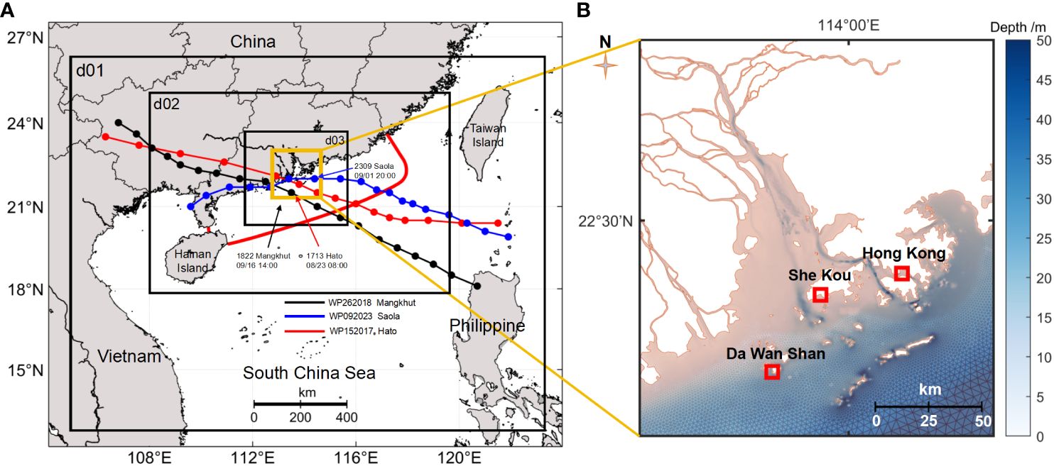
Figure 1 Overview of the study area, the passage of the three typhoons, and model domain. (A) The corresponding three nested regions (d01, d02, and d03 marked by black rectangles) in the WRF simulation (red, white, and green dotted lines mark the paths of Hato, Mangkhut, and Saola, respectively), the ADCIRC simulation (surrounded by bold red lines). (B) close-up of the estuary [marked by light yellow rectangle in (A), terrain (Colour bar) in and near the PRE, and tide gauge stations (marked by red rectangles).
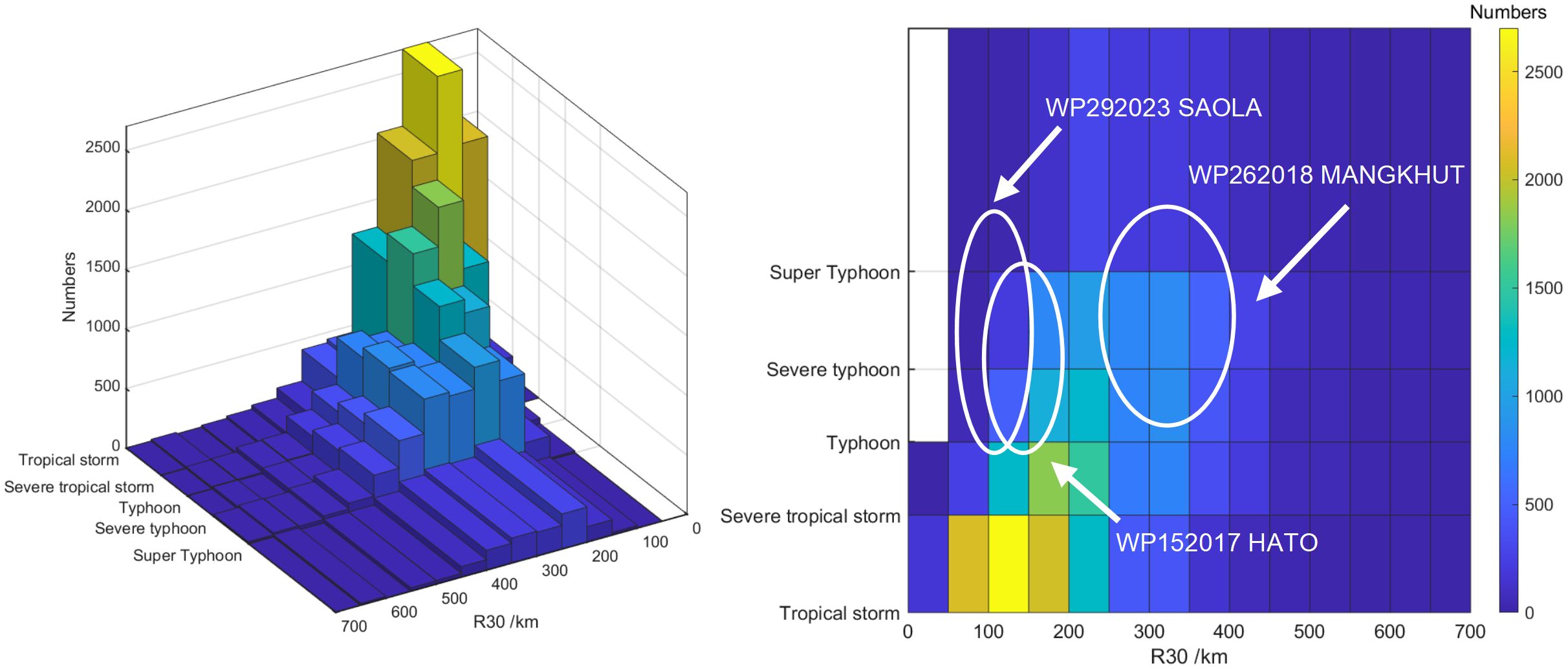
Figure 2 Statistics of different 30-knot wind radii and tropical cyclone grades from JMA TC track data (white ellipse marks the variation range of Mangkhut, Saola, and Hato).
Three represented wind fields, including (1) parametric, (2) reanalysis (3) and numerical wind fields, were implemented to evaluate the storm tide simulation, and to provide data for LSTM training. In the following sections, the three wind fields are described in detail.
The Willoughby and Rahn (2004) formula (Equation 1, referred to as Wil hereinafter) was used to calculate Rmax, which has been developed successfully for storm tide simulation in the Pearl River Estuary (Yang et al., 2019; Jian et al., 2021; Du et al., 2023). We then constructed the dynamic Holland wind field for three TC based on Fleming et al. (2008) method (Equations 1, 2). Other parameters including LON, LAT, Pres and Vmax were obtained from the JMA and NMC dataset. Another improved parametric wind field is described in detail in section 3.1.
where Penv is the atmospheric pressure, r is the distance to the TC centre, P is the atmospheric pressure at a distance r from the TC centre, and Vg is the wind velocity at a distance r from the TC centre.
The fifth-generation ECMWF reanalysis for global climate and weather data (ERA5) was applied for 10-m wind speed and sea level pressure (https://cds.climate.copernicus.eu/cdsapp#!/dataset/reanalysis-era5-single-levels?tab=form). This dataset has a temporal and spatial resolution of 1 h and 0.25° × 0.25°, respectively. The reanalysis data were interpolated to a grid resolution of 0.1° × 0.1° using the natural neighbour method for further interpolation.
The Weather Research and Forecasting Model (WRF) was used to produce numerical wind fields of Hato (2017) and Mangkhut (2018). Our simulation contained 45 pressure levels and three nested domains (d01, d02 and d03, shown in Figure 1). The horizontal grid spacing was 18, 6, and 2 km for d01, d02, and d03, respectively. Table 1 shows the parameterisation schemes used in the WRF simulation. The microphysics scheme adopted the WSM6-class, while the shortwave and longwave radiation were obtained from the RRTMG. The boundary layer scheme followed the MYJ, the convective parameterisation adopted the Grell–Freitas scheme, the land surface scheme used the Noah scheme, and the surface parameterisation used the Eta Similarity scheme (Li, 2012; Dong et al., 2021). The 0.25° × 0.25° NCEP-FNL data were used as the initial field. The Hato simulation run from 21 August 2017 at 00:00 to 25 August 2017 at 00:00, and the Mangkhut simulation run from 14 September 2018 at 00:00 to 18 September 2018 at 00:00.
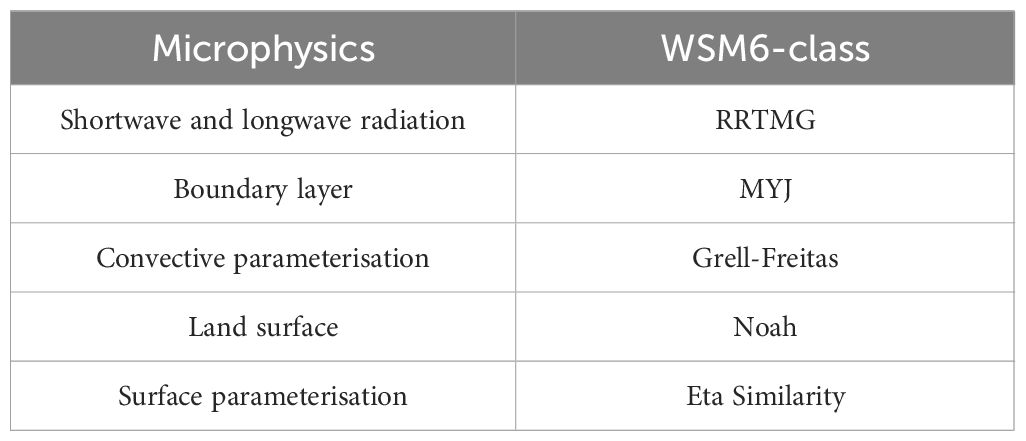
Table 1 Parameterisation schemes used in WRF.
The root mean square error (RMSE), correlation coefficient (CC), peak error, and trough error were used to evaluate the simulation performance (Equations 3–5). Smaller values of RMSE and peak/trough error and higher values of r indicated better agreement. These metrics are defined as follows:
where Xmod is the model value, Xobs is the observation value, and f is Earth’s rotation parameter. The superscript of “t_obs” represents the observation time.
The Advanced Circulation (ADCIRC) model was applied to establish a storm tide forecasting model. Our model domain covered the Pearl River Estuary, the Guangdong coast, and the adjacent shallow continental shelf (Figure 1). The model consisted of 272,632 triangular grids and 155,219 nodes, and was locally refined around the estuary. The water depths were merged by the General Bathymetric Chart of the Ocean (GEBCO) 2023 dataset and nautical charts in the Pearl River Estuary. The open boundary conditions including eight major tidal components (K1, O1, P1, S1, M2, N2, K2, and S2) were extracted from the TPXO9 tidal dataset (Egbert and Erofeeva, 2002). The tidal simulations were validated against the observations at the Hong Kong, Da Wan Shan and She Kou gauge station (Figure 3). The RMSEs at the three stations were 4.2, 3.9, and 8.68 cm, respectively, and all CCs were greater than 0.99. The good tidal results obtained serve as a strong foundation for further storm tide simulating.
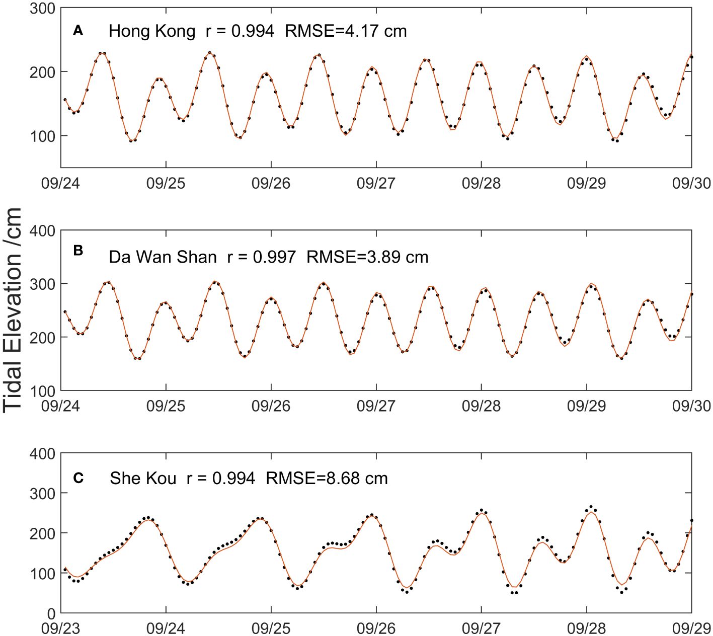
Figure 3 Simulations (line) and observations (scatter) of tidal levels at the three tidal gauge stations. (A) Hong Kong (B) Da Wan Shan (C) She Kou Station.
Big-data-driven statistics and machine learning have been applied to forecast storm tides in recent years (Ramos-Valle et al., 2021; Lockwood et al., 2022; Tian et al., 2024). LSTM is a special neural network that addresses gradient explosion and vanishing problems in conventional RNNs (Gers et al., 2000; Pascanu et al., 2013). Unlike typical feedforward neural networks, LSTM particularly suits time-series prediction. LSTM contains four units: memory cell state Ct, input gate it, forget gate ft, and output gate ot (Equation 6), which are defined as:
where , , , , and represent the input data, hidden state, temporary cell state, weight matrices, and sigmoid activation function, respectively.
The Random Forest (RF) uses decision trees as estimators based on a bagging algorithm. By combining multiple decision trees, the dataset features are randomly selected or returned with replacements for training (Brownlee, 2020). Here, the dataset was divided into training and testing parts. The training data were split into n samples. Then a bag and an out-of-bag set were constructed for each sample. A decision tree was constructed for each sample, and the predictions were recorded. All generated decision trees were combined to obtain the final RF model.
Rmax is an important parameter when constructing the Holland wind field. In addition to Wil, we incorporated a large wind radius into the Rmax calculation. Considering the TC as a rotating background, the circulation system of the boundary layer air flowed radially from the outer side to the centre (Riehl, 1954; Wing et al., 2016). In this scenario, the equation for absolute angular momentum (M) is as follows (Equations 7, 8):
R34 is related to M34 and Mmax. Rmax can be further determined with known Vmax and LAT. Thus, R34 links to Rmax. A nonlinear regression proposed by Chavas and Knaff (2022), known as Fcha, was used to solve the C15 model (Equation 9). Here, we applied MTCSWA data to determine the appropriate coefficients in the Northwest Pacific region. An additional Vmax weighting coefficient µ was introduced to improve the calculation of Rmax during strong TCs (Equation 10). Equation 11 (referred to as F34 hereafter) is the modified formula.
Compared with MTCSWA data, CC is 0.77 and RMSE is 17.7 km (Figure 4). The calculation fits well with the dataset practically in the high-wind-speed range.
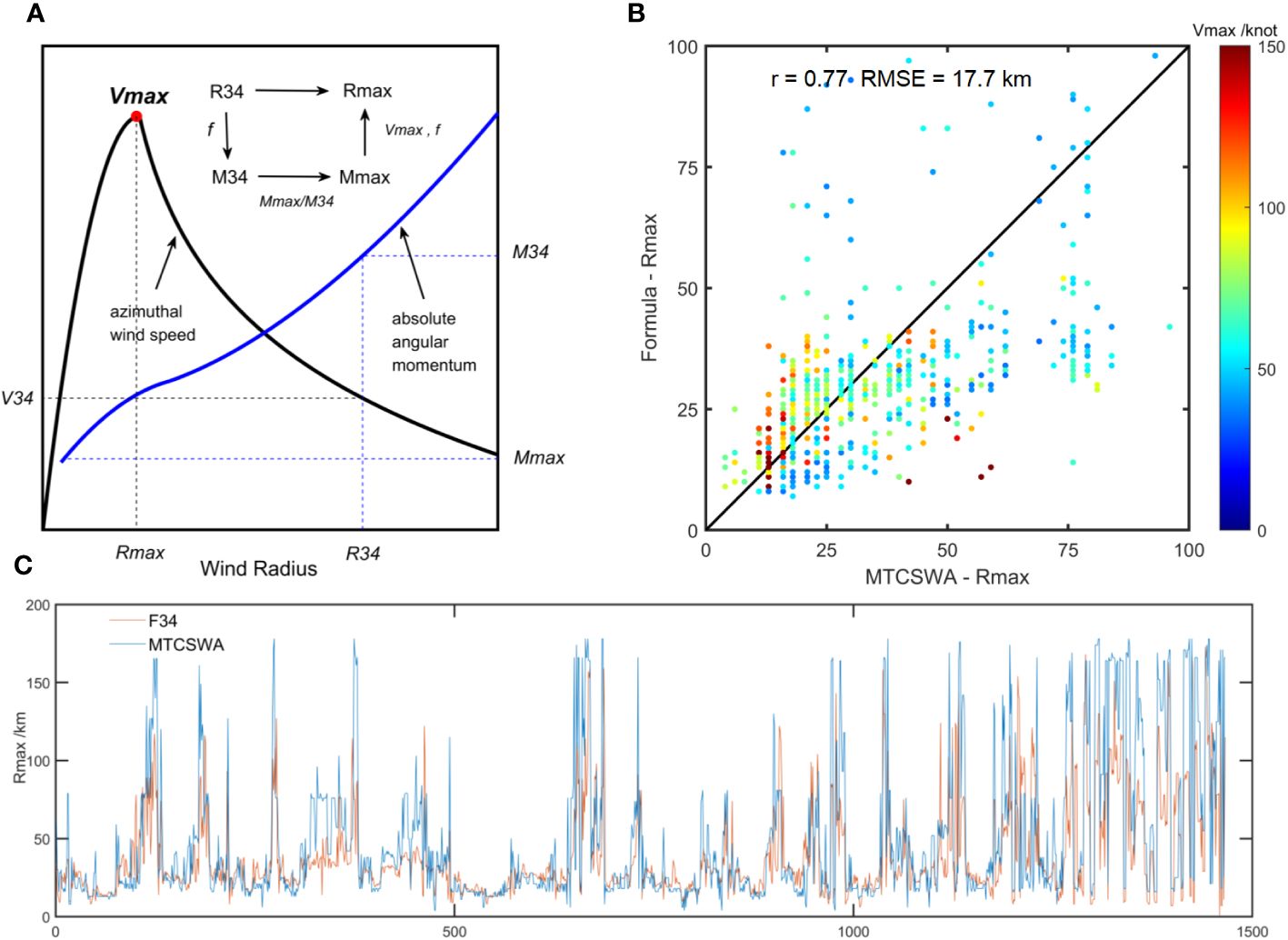
Figure 4 (A) Azimuthal wind speed (black) and absolute angular momentum (blue). (B, C) Comparisons between F34 calculated values and MTCSWA data. The scatter colour in (B) represents Vmax.
Some Asian agencies provide a 30-knot wind radius (15.5 m/s, JMA), or a category-7 wind radius (13.9–17.1 m/s, CMA) equivalent to the 30-knot wind radius. Therefore, R30 needs to be converted to R34 based on certain functional relationships. Here, we implemented the Rankine vortex scheme to determine the proportional relationship between R30 and R34 (Equations 12–14). The scheme consists of a solid rotating region with constant vorticity or angular momentum at its centre surrounded by zero-vorticity circulation. The angular momentum loss due to surface friction during typhoons can be assumed to be less than one (Riehl, 1954). The values were set to 0.5 after the typhoon landfall and 0.8 in the open sea.
To evaluate the performance on storm tide simulation, we conducted simulations based on new F34 and previous Fcha data. During Hato and Mangkhut, F34 yielded better results for peak errors (Figure 5). The maximum error eliminated was up to 20 cm, which indicates that the modified Rmax calculation can conduct better simulations.
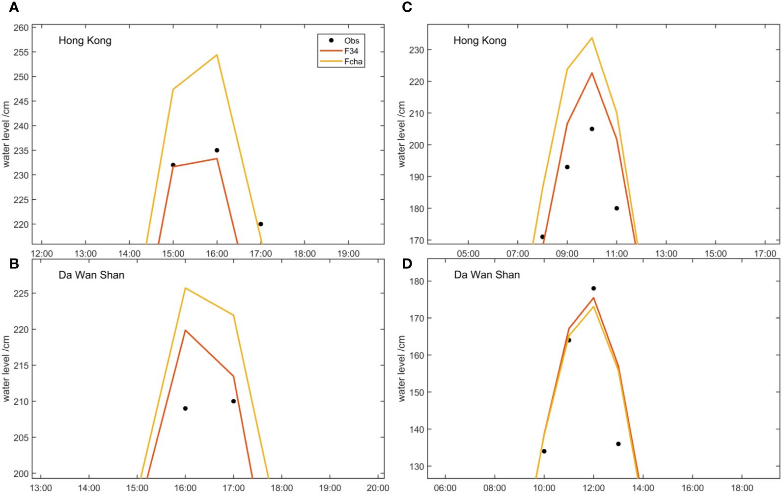
Figure 5 Comparisons of water level between F34 and Fcha during the Mangkhut and Hato periods. (A, B) Mangkhut’s and (C, D) Hato’s peak water levels.
In the previous sections, we described four ways to construct a wind field during strong typhoons. Parametric wind fields based on F34 and Wil, numerical wind fields using WRF, and reanalysis wind fields from ERA5 were then implemented into ADCIRC to carry out the storm tide simulations. ERA5 and WRF wind data were provided at hourly intervals. To avoid specific time errors caused by different minute–averaging methods among JMA, C15, and other dataset, Wil and F34 data, which have a longer time interval, were provided every 6 h. To adjust tidal elevation, the simulations ran for three days from a cold start. Subsequently, the storm tides during super typhoon Mangkhut (15–18 September 2018) and severe typhoon Hato (22–25 August 2017) were simulated based on well-adjusted tide data.
Figure 6 shows the simulated results and Table 2 shows the performance metrics. During super typhoon Mangkhut, the CCs between F34 and the observation both exceeded 0.94. F34 also shows the smallest peak error (1.7 cm at Hong Kong and -3.46 cm at Da Wan Shan) and trough error (13.31 cm at Hong Kong and 5.9 cm at Da Wan Shan). Conversely, the simulation based on WRF wind shows a higher water level than the observation, with peak errors of -22.6 and -25.7 cm at the two stations, respectively. The simulation based on Wil wind resulted in a lower water level, with peak errors reaching 27.7 and 14.15 cm at the two stations, respectively. Additionally, both WRF and Wil showed poor performance during the receding period, with much higher trough errors (Table 2).

Figure 6 Comparisons between simulations and observations of WRF, Wil, ERA5, and F34. (A) Hong Kong (B) Da Wan Shan during Mangkhut and (C) Hong Kong (D) Da Wan Shan during Hato.
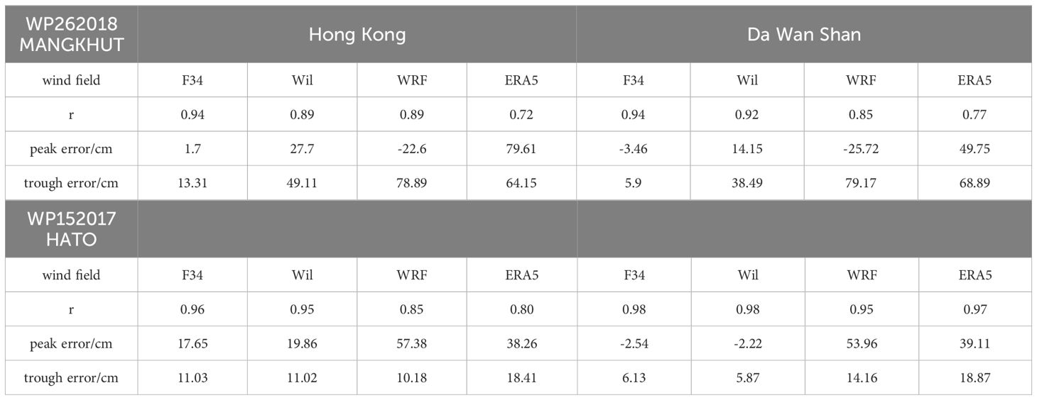
Table 2 Performance metrics of Mangkhut and Hato.
During the severe typhoon Hato period, the performances of F34 and Wil were similar. Both accurately simulated the water level surge and recession closely matching the observations. In contrast, WRF simulated relatively larger peaks and trough errors (Table 2). Additionally, the simulation based on ERA5 showed poor performance for both TCs, indicating that it is not suitable for storm tide forecasting during strong TCs.
According to the metrics, F34 effectively reproduced the storm tides during the two TC events. It not only outperformed other wind fields (WRF and ERA5), but it also reduced the simulation error compared to the commonly used Wil model. Although the results for Hato showed good agreement with the observations, the simulated results for F34 and Wil were almost identical.
Figure 7 shows spatial distributions of peak and trough water levels. The water level at Hong Kong changed approximately 2 h faster than that at Da Wan Shan during Mangkhut. The time of the extreme water level at Hong Kong was used as time reference. The peak water level order is WRF > F34 ≈ Obs > Wil, and the trough water level order is WRF< Wil< F34 ≈ Obs. This further proves that F34 yields a more reasonable simulation. Therefore, the introduction of large wind radius to calculate Rmax in strong TCs is necessary to simulate storm tides using parametric wind fields.
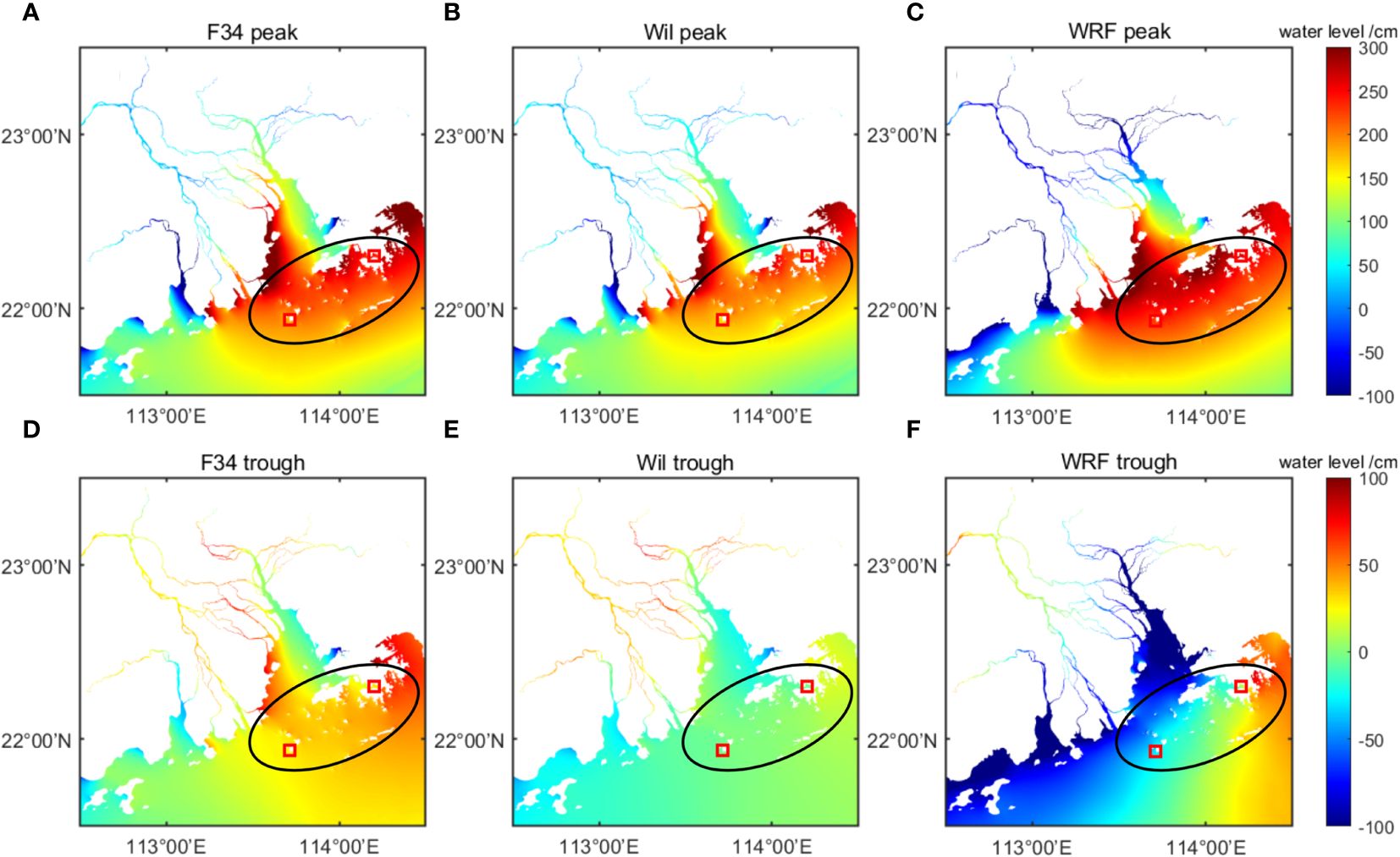
Figure 7 Spatial distribution of peak (A–C) and trough water levels (D–F) during Mangkhut in the Pearl River Estuary. The red box represents two observation stations.
Due to the better constraint on Rmax calculation provided by the C15 model, the Holland wind field using F34 exhibited the highest performance. We calculated Rmax for TCs at 6-h intervals from 1977 to 2023 in the Northwest Pacific region using the F34 formula. These calculated data were then used to train an LSTM network and forecast Rmax for the next 6, 12, 24, 36, and 48 h separately (Figure 8). The training data span from 1977 to 2014, comprising 22,655 samples. The validation data covered the period from 2015 to 2021 with 4,127 samples. The testing data included 903 samples from 2022 to 2023.
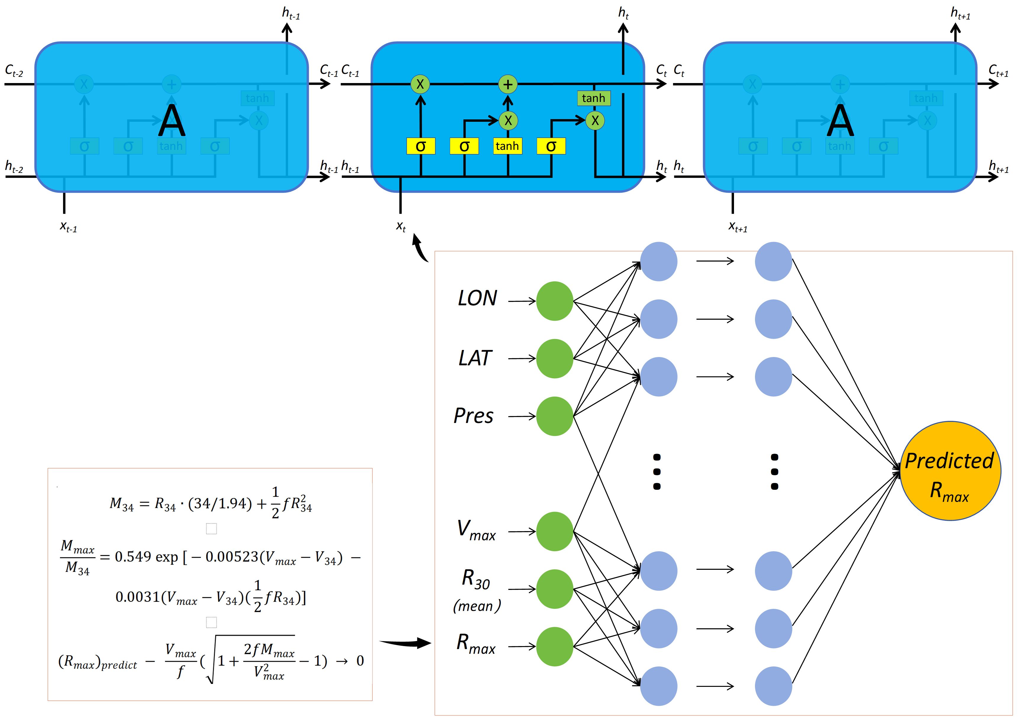
Figure 8 LSTM network diagram.
The specific settings of our LSTM model were as follows:
The input layer included six parameters: LAT, LON, Pres, Vmax, averaged R30, and Rmax. The outputs were Rmax for the next 6, 12, 24, 36, and 48 h. The hidden layer contained 128 neurons. The number of epochs was set to 200, the activation function was ‘Relu’, the initial learning rate was 0.005, the dropout value was 0.1, and the training algorithm was the ‘Adam’ optimisation. Each network was trained 10 times. The output of the LSTM model was compared with testing data (Figure 9). The CCs were 0.994, 0.913, 0.740, 0.577, and 0.434, respectively. The RMSEs were 3.64, 10.02, 16.17, 19.68, and 21.75 km, respectively. These results indicate that the neural network can accurately capture the patterns of Rmax and forecast its future values.
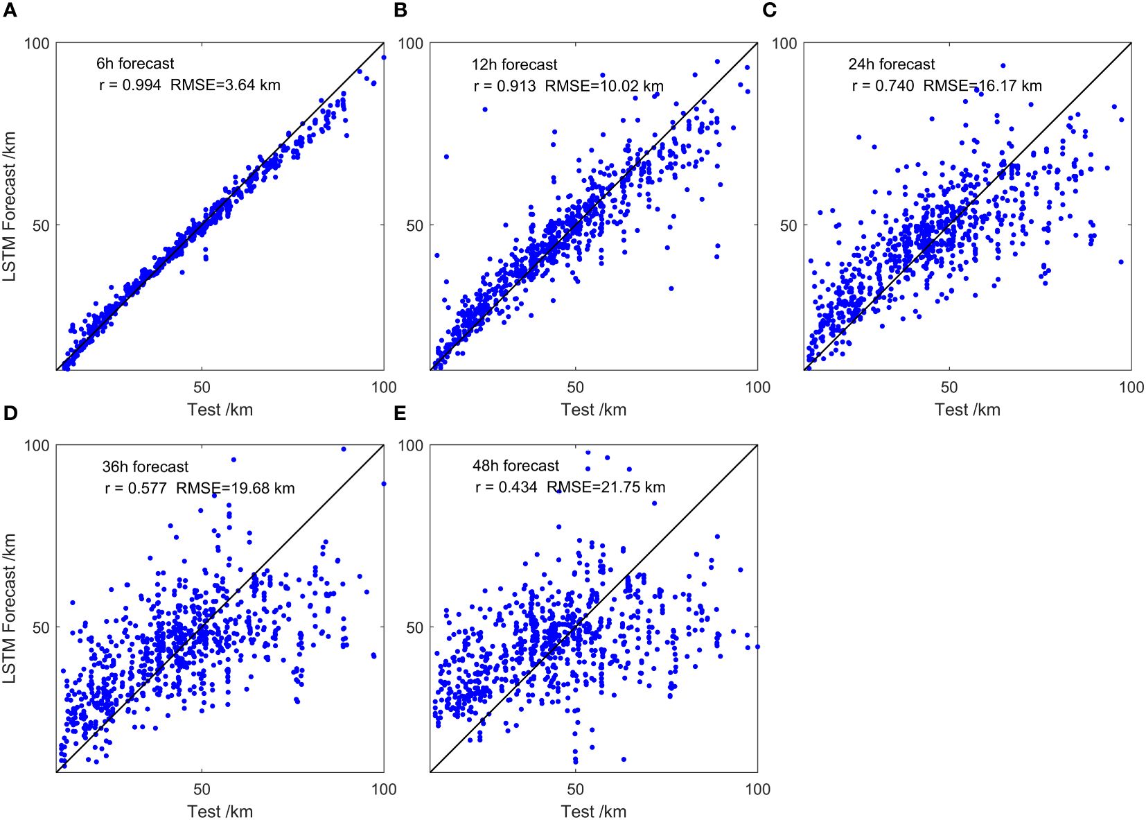
Figure 9 LSTM test data results in (A) 6-h (B) 12-h, (C) 24-h, (D) 36-h, and (E) 48-h forecasts.
To further test the applicability of our neural network, we conducted a forecast experiment using JMA data during super typhoon Saola. The forecasted Rmax was compared with F34, Wil, and the ATCF Tropical Cyclone Database (Figure 10). At 6 and 12 h, the forecasted Rmax matched F34 very well, with only slight differences observed at 24 and 36 h. However, the trend and magnitude at 24 and 36 h fit well with ATCF. Although the bias increased at 48 h, the values remained within a reasonable range.
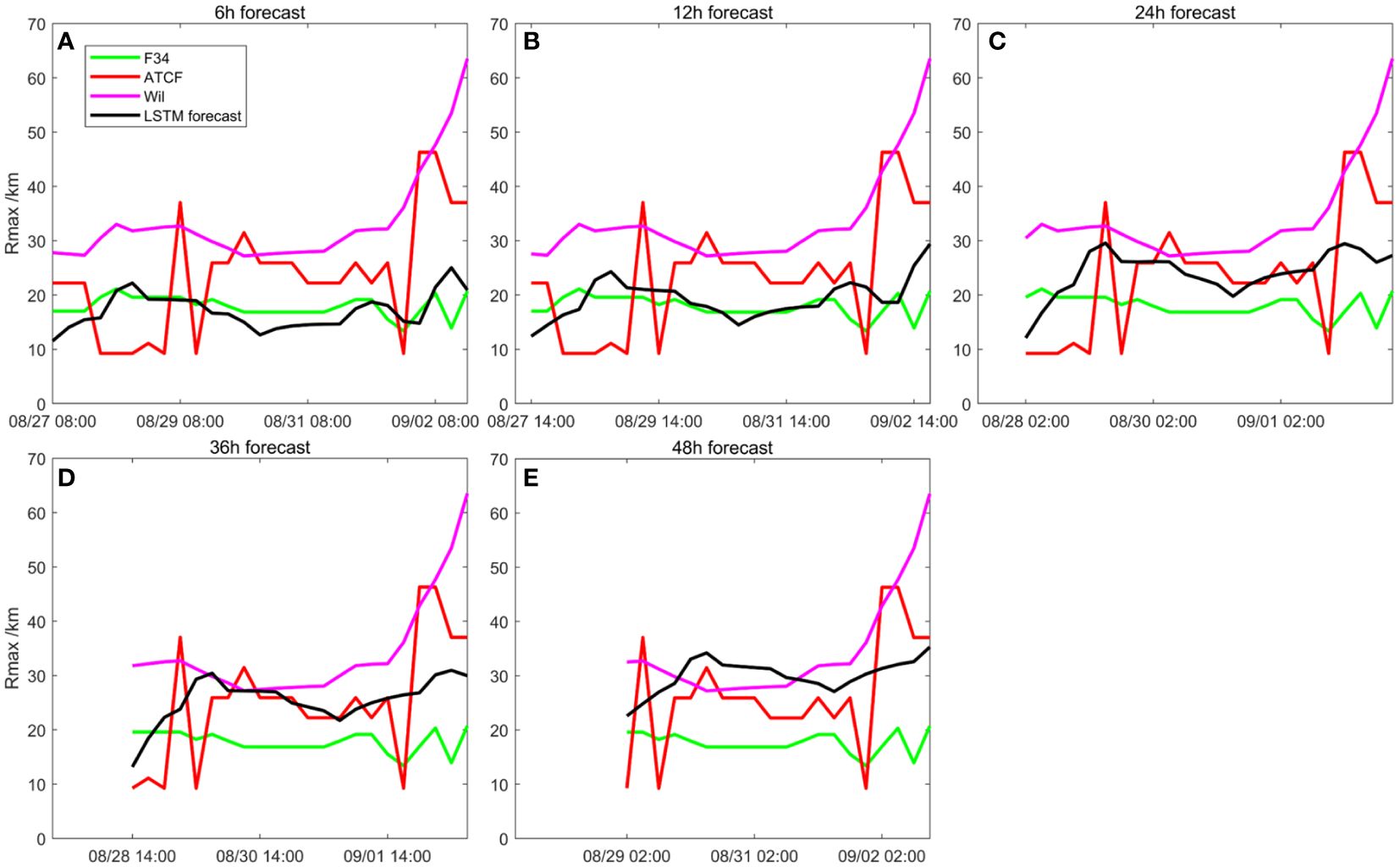
Figure 10 LSTM’s forecasting Rmax results during super typhoon Saola compared with F34, the Wil hindcast value, and the ATCF dataset. (A) 6-h (B) 12-h, (C) 24-h, (D) 36-h, and (E) 48-h forecasts.
We then simulated the storm tide during Saola based on the forecasted Rmax. Figure 11 and Table 3 show the simulation results. Compared with the observations, F34 still shows the best performance, followed by the 6, 12, 24, 36, and 48-h forecasts, with Wil showing the worst performance. For the 6-h forecast, the CCs were 0.96 and 0.94 at the two stations, respectively, while the RMSEs were 18.1 and 22.4 cm, respectively. The peak errors were 14.4 and 26.4 cm, respectively. As the forecasting hours increased, the errors grew. For the 48-h forecast, the CCs were 0.87 and 0.86, the RMSEs were 32.05 and 39.80 cm, and the peak errors were 29.39 and 41.59 cm. This result not only confirms the improvement of using the F34 method in simulating storm tide during strong TCs, but also demonstrates that constraining the neural network with the C15 model for prediction is feasible.
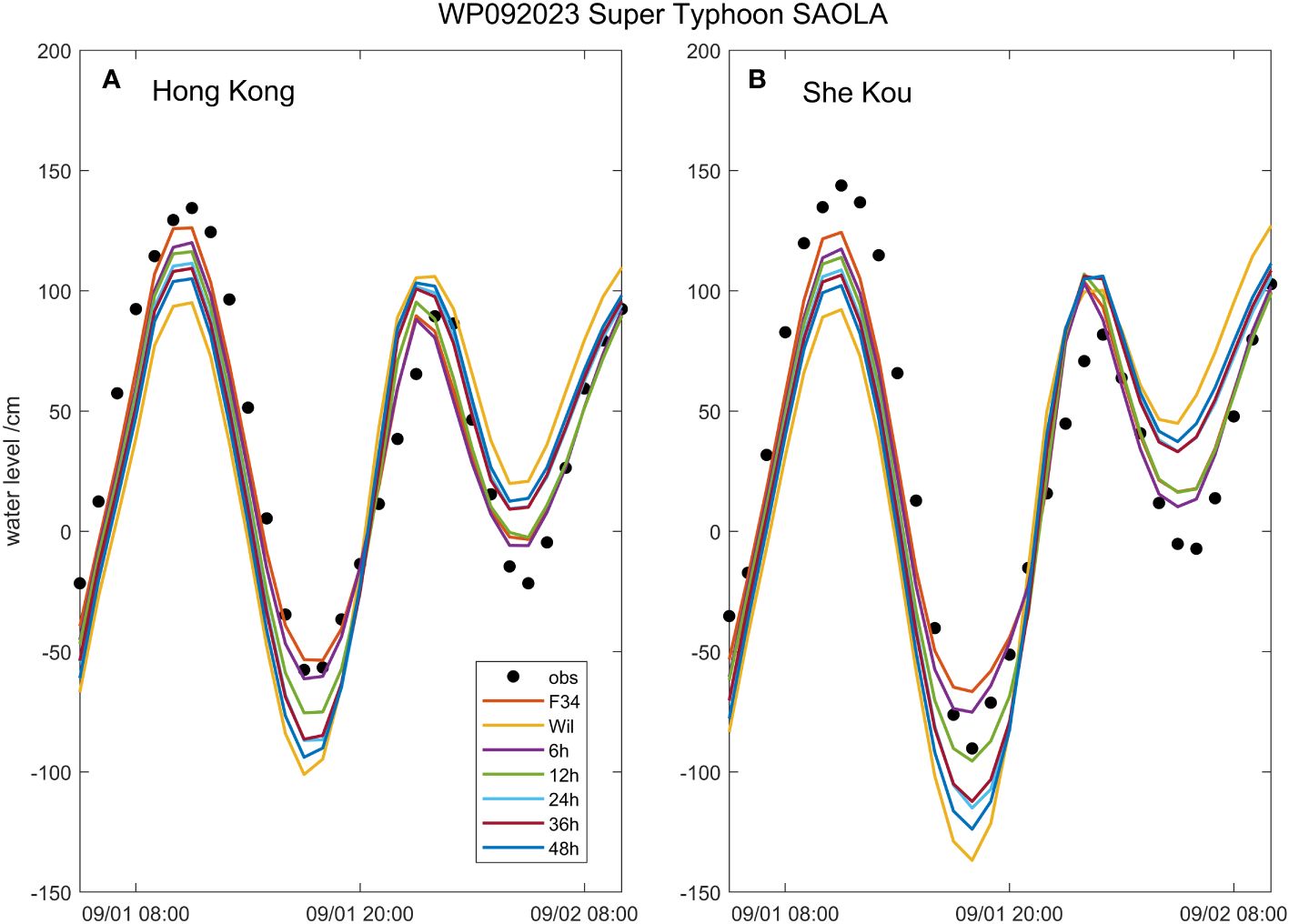
Figure 11 Simulated water level (line) during super typhoon Saola compared with observation data (scatter) in the (A) Hong Kong and (B) She Kou stations.
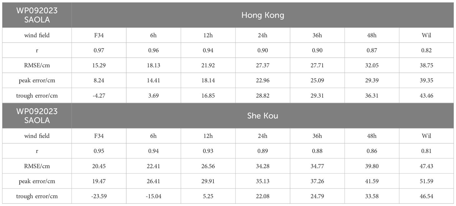
Table 3 Performance metrics of Saola.
The feature importance output from the RF can be used to determine which input features are effective in predicting the target variable (Brownlee, 2020). After filtering and excluding the data from MTCSWA, a total of 1,719 valid timestamps were obtained. Among these, 1,512 timestamps were used as the training data, and 207 timestamps were used as the test data. Our RF model comprised 100 decision trees, with a minimum number of five leaves per tree, and performed regression calculation. The sum of the feature importance values for all input features was equal to 1, where higher importance values indicated greater significance of that feature in the RF model (Pedregosa, 2011).
Figure 12 displays the feature importance coefficients and the correlation coefficient matrix obtained by training the RF using five input features: LON, LAT, Pres, R34, and Vmax. The impact of R34 on Rmax was highest, exceeding 40%. LAT was the second important feature, and Vmax was the third. The RF results suggest that the large wind radius was closely related to Rmax and affected its prediction. This conclusion explains why introducing the C15 model improves the hindcast and LSTM forecasting performance for strong TCs. The main reason is that the large wind radius is considered, unlike in other formulas (Table 4). Additionally, the correlation between R34 and Rmax was positive, whereas the correlation between Vmax and Rmax was negative. The F34 formula also aligned with these correlation signs.
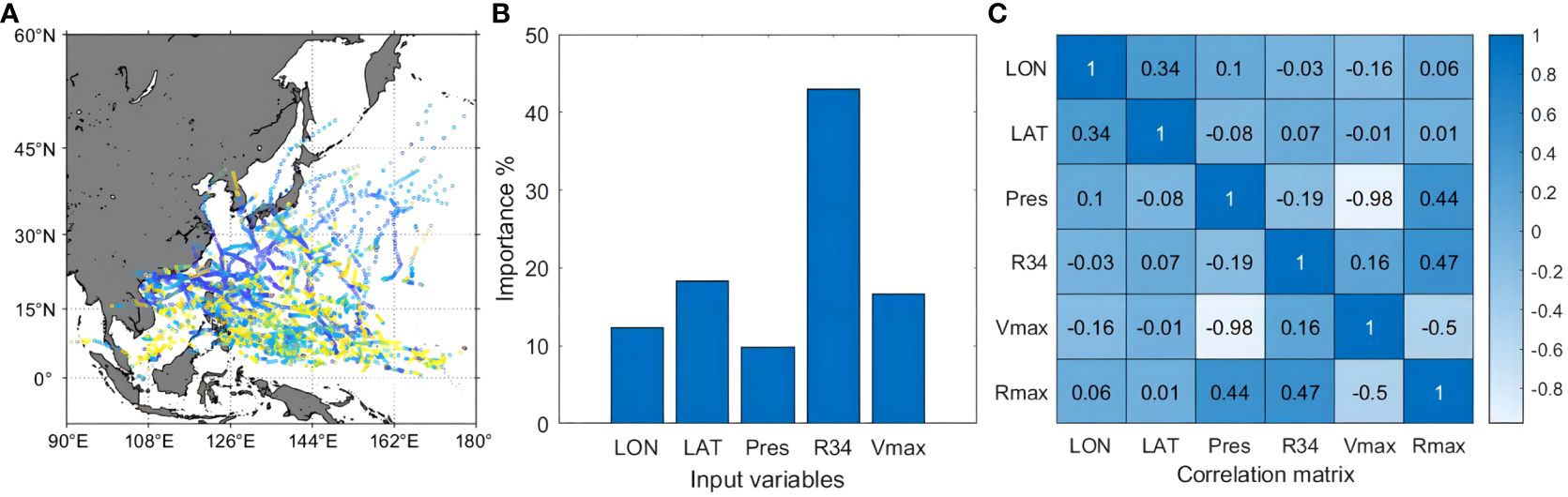
Figure 12 (A) MTCSWA TC data in the Northwest Pacific during the period from 2022 to 2023. Importance (B) and correlation matrices (C) of several input variables in the RF model.
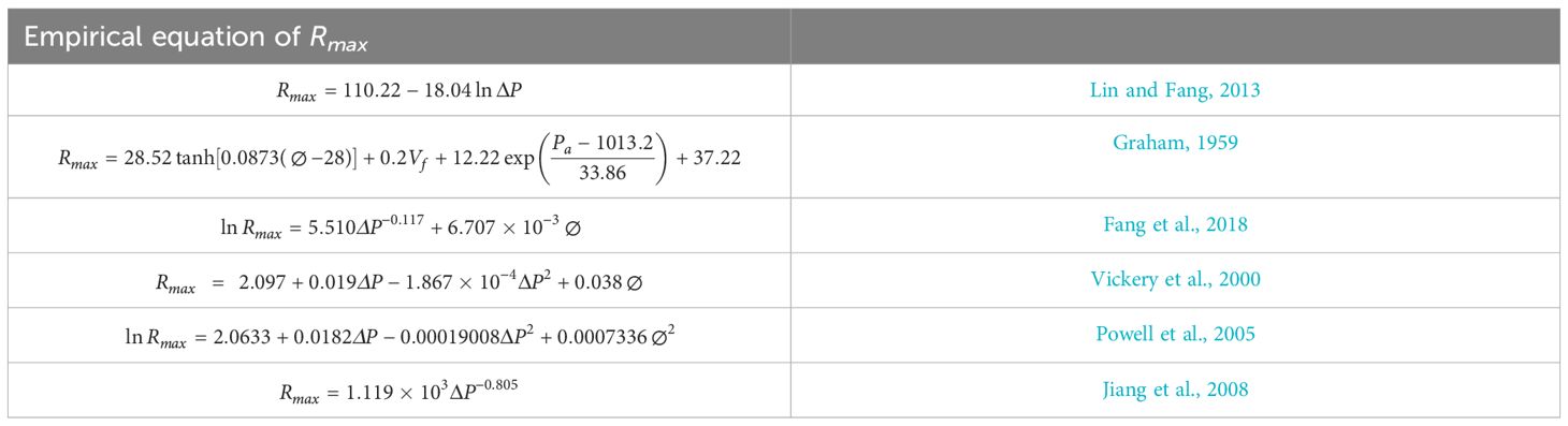
Table 4 Empirical equations for calculating Rmax.
As mentioned in Section 3.2, the storm tide forecasting by introducing the large wind radius has certain applicability conditions. The improvement effectively increased the accuracy of storm tide predictions during Mangkhut and Saola, but had little impact on Hato. In the above study, we confirmed that R34 plays a crucial positive role in Rmax estimation, and Rmax is important for storm surge prediction (Irish et al., 2008). However, few institutions and datasets provide Rmax data in the Northwest Pacific region. Due to the limited number of samples and the duration of MTCSWA, we continued to use the same training and testing sets as those used for the LSTM network training. Based on the input parameters of LON, LAT, Vmax, and Pres, a regression prediction for R30 can be made. The disadvantage, similar to other simple empirical formulas, is that the RF’s training data or the model itself also lack physical constraints.
Figure 13 shows the final training and testing results using the RF model. Both sets of results exhibited a notable phenomenon: the regression performed well when R30 was in the range of 100–300 km; however, when it was larger than 300 km, the regression consistently underperformed, predicting lower values than actual. Similarly, when R30 was less than 100 km, the predicted results tended to be higher than the target values. As Mangkhut began to affect the Pearl River Estuary at 8:00 a.m. on 16 September, the Rmax calculated by F34 was 49 km, whereas Wil estimated it to be only 30 km. Additionally, as Saola affected the Pearl River Estuary at 2:00 p.m. on 1 September, the Rmax calculated by F34 was 16 km, while Wil estimated it to be 32 km. This situation aligns with the results of the RF model, as Mangkhut is a rare large super typhoon and Saola is a smaller one. The different ranges of large wind radii resulted in noticeable differences in Rmax, ultimately leading to higher errors in water level modelling using the Wil method during the Mangkhut and Saola periods. Therefore, it is necessary to incorporate a large wind radius into numerical prediction by combining the empirical formula and artificial intelligence as suggested in this study. It should be noted that this study does not aim to comprehensively identify the best parameter based on the C15 model with the highest accuracy. Although our model improves the extreme storm tide forecasting, the investigation of other physical parameters on storm tide forecasting is a subject for future work.
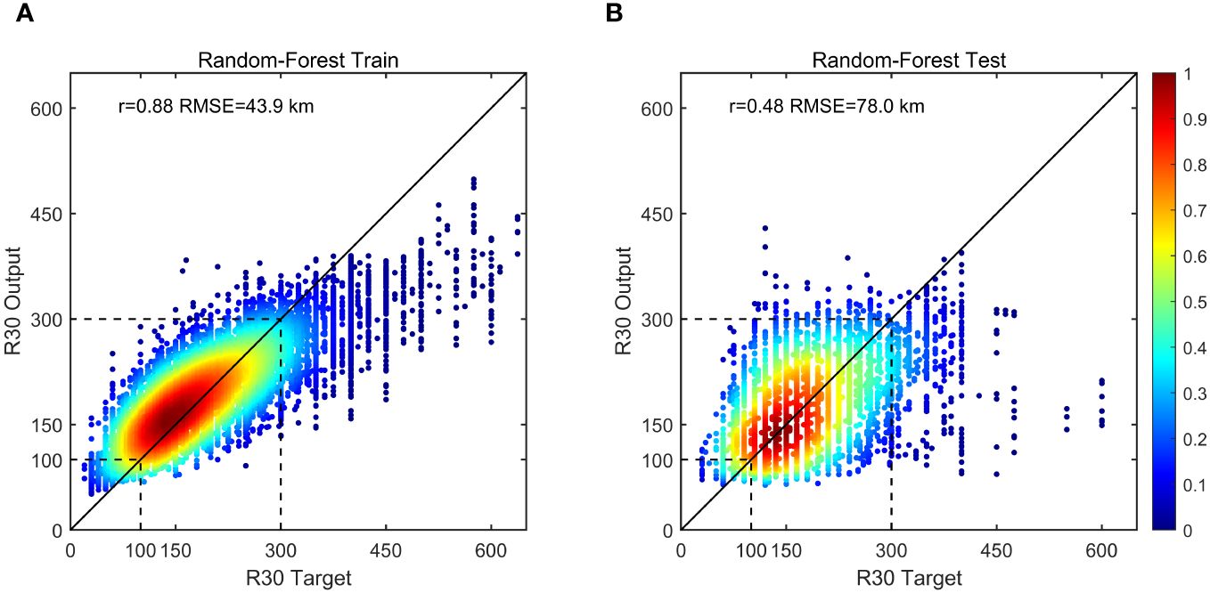
Figure 13 Random Forest training (A) and testing r (B). The coloured scatter marks the output data’s distribution density.
In this study, we optimised a nonlinear regression based on the C15 model for determining the maximum wind radius. We then evaluated storm simulations using ADCIRC with a parametric wind field based on the improved regression, along with other wind fields, during super typhoon Mangkhut (WP262018) and severe typhoon Hato (WP152017). Additionally, we attempted to forecast Rmax for up to 48 h using an LSTM neural network. The forecasting performance of the LSTM model was tested during super typhoon Saola (WP092023).
As the large wind radius positively correlates with Rmax and can better determine the TC size compared to other regular TC parameters, the improved C15 model can accurately simulate storm tides during strong TCs. Moreover, the modified formula appears to be more suitable for the Northwest Pacific region during strong typhoons. The physically constrained LSTM effectively forecasts parameters during TCs, making the numerical results more reasonable and reliable. Based on the analysis in this study, we suggest that combing a physics-based wind profile model with artificial intelligence is an effective good method for forecasting storm tides induced by strong typhoons. Given the significant improvement in storm tide forecasting for strong TCs, it is necessary to apply this method in marine disaster warning systems.
The original contributions presented in the study are included in the article/supplementary material. Further inquiries can be directed to the corresponding author.
YW: Writing – original draft. JL: Writing – review & editing. LX: Writing – review & editing. TZ: Writing – review & editing. LW: Writing – review & editing.
The author(s) declare financial support was received for the research, authorship, and/or publication of this article. This study was supported by Independent Research Project of Southern Marine Science and Engineering Guangdong Laboratory (Zhuhai), China (SML2022SP301), National Natural Science Foundation of China (42276019, 41976018), Program for Scientific Research Start-up Funds of Guangdong Ocean University (060302032106, 060302032202).
The authors declare the research was conducted in the absence of any commercial or financial relationships that could be construed as a potential conflict of interest.
All claims expressed in this article are solely those of the authors and do not necessarily represent those of their affiliated organizations, or those of the publisher, the editors and the reviewers. Any product that may be evaluated in this article, or claim that may be made by its manufacturer, is not guaranteed or endorsed by the publisher.
Bajo M., De Biasio F. D., Umgiesser G., Vignudelli S., Zecchetto S. (2017). Impact of using scatterometer and altimeter data on storm surge forecasting. Ocean Model. 113, 85–94. doi: 10.1016/j.ocemod.2017.03.014
Bass B., Irza J. N., Proft J., Bedient P., Dawson C. (2017). Fidelity of the integrated kinetic energy factor as an indicator of storm surge impacts. Natural Hazards 85, 575–595. doi: 10.1007/s11069-016-2587-3
Bruneau N., Polton J., Williams J., Holt J. (2020). Estimation of global coastal sea level extremes using neural networks. Environ. Res. Lett. 15, 074030. doi: 10.1088/1748-9326/ab89d6
Chang D., Amin S., Emanuel K. (2020). Modeling and parameter estimation of hurricane wind fields with asymmetry. J. Appl. Meteorology Climatology 59, 687–705. doi: 10.1175/jamc-d-19-0126.1
Chavas D. R., Knaff J. A. (2022). A simple model for predicting the tropical cyclone radius of maximum wind from outer size. Weather Forecasting 37, 563–579. doi: 10.1175/WAF-D-21-0103.1
Chavas D. R., Lin N., Emanuel K. (2015). A model for the complete radial structure of the tropical cyclone wind field. Part I: Comparison with observed structure. J. Atmospheric Sci. 72, 3647–3662. doi: 10.1175/jas-d-15-0014.1
Cyriac R., Dietrich J. C., Fleming J. G., Blanton B. O., Kaiser C., Dawson C. N., et al. (2018). Variability in coastal flooding predictions due to forecast errors during hurricane Arthur. Coast. Eng. 137, 59–78. doi: 10.1016/j.coastaleng.2018.02.008
Deppermann C. E. (1947). Notes on the origin and structure of Philippine typhoons (399-404: Bulletin of the American Meteorological Society).
Ding Y., Ding T., Rusdin A., Zhang Y., Jia Y. (2020). ). Simulation and prediction of storm surges and waves using a fully integrated process model and a parametric cyclonicwind model. J. Geophys. Res.: Oceans 125, e2019JC015793. doi: 10.1029/2019jc015793
Dong W., Feng Y., Chen C., Wu Z., Xu D., Li S., et al. (2021). Observational and modeling studies of oceanic responses and feedbacks to typhoons Hato and Mangkhut over the northern shelf of the South China Sea. Prog. Oceanography 191, 102507. doi: 10.1016/j.pocean.2020.102507
Du H., Yu P., Zhu L., Fei K., Gao L. (2023). Assessing the performances of parametric wind models in predicting storm surges in the Pearl River Estuary. J. Wind Eng. Ind. Aerodynamics 232, 105265. doi: 10.1016/j.jweia.2022.105265
Egbert G. D., Erofeeva S. Y. (2002). Efficient inverse modeling of barotropic ocean tides. J. Atmos. Ocean Technol. 19, 183–204.
Fang G., Zhao L., Song L., Liang X., Zhu L., Cao S., et al. (2018). Reconstruction of radial parametric pressure field near ground surface of landing typhoons in Northwest Pacific Ocean. J. Wind Eng. Ind. Aerodynamics 183, 223–234. doi: 10.1016/j.jweia.2018.10.020
Fang P., Ye G., Yu H. (2020). A parametric wind field model and its application in simulating historical typhoons in the western North Pacific Ocean. J. Wind Eng. Ind. Aerodynamics 199, 104131. doi: 10.1016/j.jweia.2020.104131
Fleming J. G., Fulcher C. W., Luettich R. A., Estrade B. D., Allen G. D., Winer H. S., et al. (2008). A real time storm surge forecasting system using ADCIRC. Estuar. Coast. modeling 2007), 893–912. doi: 10.1061/40990(324
Gers F. A., Schmidhuber J., Cummins F. (2000). Learning to forget: Continual prediction with LSTM. Neural Comput. 12, 2451–2471.
Giaremis S., Nader N., Dawson C., Kaiser C., Nikidis E., Kaiser H., et al. (2024). Storm surge modeling in the AI era: Using LSTM-based machine learning for enhancing forecasting accuracy. Coast. Eng. 191, 104532. doi: 10.1016/j.coastaleng.2024.104532
Gori A., Lin N., Schenkel B., Chavas D. (2023). North atlantic tropical cyclone size and storm surge reconstructions from 1950-present. J. Geophysical Research: Atmospheres 128, e2022JD037312. doi: 10.1029/2022JD037312
Graham H. E. (1959). Meteorological Considerations Pertinent to Standard Project Hurricane, Atlantic and Gulf Coasts of the United States (Washington, D. C: U. S. Department of Commerce, Weather Bureau).
He J., He Y., Li Q., Chan P. W., Zhang L., Yang H. L., et al. (2020). Observational study ofwind characteristics, wind speed and turbulence profiles during Super Typhoon Mangkhut. J. Wind Eng. Ind. Aerod. 206, 104362. doi: 10.1016/j.jweia.2020.104362
Hinkel J., Lincke D., Vafeidis A. T., Perrette M., Nicholls R. J., Tol R. S. J., et al. (2014). Coastal flood damage and adaptation coats under 21st century sea-level rise. Proc. Natl. Acad. Sci. 111, 3292–3297. doi: 10.1073/pnas.1222469111
Holland G. J. (1980). An analytic model of the wind and pressure profiles in hurricanes. Monthly Weather Rev., 1212–1218. doi: 10.1175/1520-0493(1980)108<1212:AAMOTW>2.0.CO;2
Irish J., Resio D., Ratcliff J. (2008). The influence of storm size on hurricane surge. J. Phys. Oceanography 38, 2003–2013. doi: 10.1175/2008JPO3727.1
Jelesnianski C. P. (1965). A numerical calculation of storm tides induced by a tropical storm impinging on a continental shelf. Monthly Weather Rev. 93, 343–358. doi: 10.1175/1520-0493(1993)093<0343:ANCOS>2.3.CO;2
Jian W., Lo E. W. M., Pan T. C. (2021). Probabilistic storm surge hazard using a steady-state surge model for the Pearl River Delta Region, China. Sci. Total Environ. 801, 149606
Jiang Z., Hua F., Qu P. (2008). A new scheme for adjusting the tropical cyclone parameters. Adv. Mar. Sci. 26, 1–7.
Kohno N., Dube S. K., Entel M., Fakhruddin S. H. M., Greenslade D., Leroux M-. D., et al. (2018). Recent progress in storm surge forecasting. Trop. Cyclone Res. Rev. 7, 128–139. doi: 10.6057/2018TCRR02.04
Landsea C. W., Franklin J. L. (2013a). Atlantic hurricane database uncertainty and presentation of a new database format. Monthly Weather Rev. 141, 3576–3592. doi: 10.1175/mwr-d-12-00254.1
Landsea C. W., Franklin J. L. (2013b). Atlantic hurricane database uncertainty and Lonentation of a new database format (National Hurricane Center). Available at: https://www.nhc.noaa.gov/data/%23hurdat.
Le X., Ho H. V., Lee G., Jung S. (2019). Application of long short-term memory (LSTM) neural network for flood forecasting. Water 11, 1387. doi: 10.3390/w11071387
Li X. (2012). The influence of the cumulus parameterization scheme in the WRF model on the simulation of typhoon tracks and intensities in the Northwest Pacific. Sci. China Press 12), 1966–1978.
Li L., Kareem A., Xiao Y., Song L., Zhou C. (2015). A comparative study of field measurements of the turbulence characteristics of typhoon and hurricane winds. J. Wind Eng. Ind. Aerod. 140, 49–66. doi: 10.1016/j.jweia.2014.12.008
Lin N., Chavas D. (2012). On hurricane parametric wind and applications in storm surge modeling. J. Geophys. Res. Atmos. 117. doi: 10.1029/2011jd017126n/a-n/a
Lin W., Fang W. (2013). Regional characteristics of Holland B parameter in typhoon wind field model for Northwest Pacific. Trop. Geogr. 33, 124–132.
Lockwood J. W., Lin N., Oppenheimer M., Lai C-. Y. (2022). Using neural networks to predict hurricane storm surge and to assess the sensitivity of surge to storm characteristics. J. Geophysical Research: Atmospheres 127, e2022JD037617. doi: 10.1029/2022JD037617
McGranahan G., Balk D. L., Anderson B. (2007). The risking tide: assessing the risks of climate change and human settlements in low elevation coatal zones. Environ. Urban. 19, 17–37. doi: 10.1177/0956247807076960
Mosavi A., Ozturk P., Chau K.-W. (2018). Flood prediction using machine learning models: Literature review. Water 10, 1536. doi: 10.3390/w10111536
Muis S., Verlaan M., Winsemius H. C., Aerts J. C. J. H., Ward P. J. (2016). A global reanalysis of storm surges and extreme sea levels. Nat. Commun. doi: 10.1038/ncomms11969
Needham H. F., Keim B. D., Sathiaraj D. (2015). A review of tropical cyclone-generated storm surges: Global data sources, observations, and impacts. Rev. Geophys. 53, 545–591. doi: 10.1002/2014RG000477
Olfateh M., Callaghan D. P., Nielsen P., Baldock T. E. (2017). Tropical cyclone wind field asymmetry-Development and evaluation of a new parametric model. J. Geophysical Research: Oceans 122, 458–469. doi: 10.1002/2016jc012237
Pandey S., Rao A. D., Haldar R. (2021). Modeling of coastal inundation in response to a tropical cyclone using a coupled hydraulic HEC-RAS and ADCIRC model. J. Geophysical Research: Oceans 126, e2020JC016810. doi: 10.1029/2020JC016810
Pascanu R., Mikolov T., Bengio Y. (2013). “Modeling of coastal inundation in response to a tropical cyclone using a coupled hydraulic HEC-RAS and ADCIRC model,” in On the difficulty of training recurrent neural networks 2013, 1310–1318.
Powell M., Soukup G., Cocke S., Gulati S., Morisseau-Leroy N., Hamid S., et al. (2005). State of Florida hurricane loss projection model: Atmospheric science component. J. Wind Eng. Ind. Aerodynamics 93, 651–674. doi: 10.1016/j.jweia.2005.05.008
Ramos-Valle A. N., Curchitser E. N., Bruyère C. L., McOwen S. (2021). Implementation of an artificial neural network for storm surge forecasting. J. Geophysical Research: Atmospheres 126, e2020JD033266. doi: 10.1029/2020JD033266
Rego J. L., Li C. (2009). On the importance of the forward speed of hurricanes in storm surge forecasting: A numerical study. Geophysical Res. Lett. 36. doi: 10.1029/2008GL036953
Rego J. L., Li C. (2010). Nonlinear terms in storm surge predictions: Effect of tide and shelf geometry with case study from Hurricane Rita. J. Geophysical Research: Oceans 115. doi: 10.1029/2009JC005285
Sampson C. R., Goerss J. S., Knaff J. A., Strahl B. R., Fukada E. M., Serra E. A. (2018). Tropical cyclone gale wind radii estimates, forecasts, and error forecasts for the Western North Pacific. Weather Forecasting 33, 1081–1092. doi: 10.1175/waf-d-17-0153.1
Schloemer R. W. (1954). Analysis and synthesis of hurricane wind patterns over Lake Okeechobee, Florida (Weather Bureau: US Department of Commerce).
Tadesse M., Wahl T., Cid A. (2020). Data-driven modeling of global storm surges. Front. Mar. Sci. 7, 512653. doi: 10.3389/fmars.2020.00260
Takagi H., Wu W. (2016). Maximum wind radius estimated by the 50 kt radius: improvement of storm surge forecasting over the western North Pacific. Natural Hazards Earth System Sci. 16, 705–717. doi: 10.5194/nhess-16-705-2016
Tian Q., Luo W., Tian Y., Gao H., Guo L., Jiang Y., et al. (2024). Prediction of storm surge in the Pearl River Estuary based on data-driven model. Front. Mar. Sci. 11, 1390364. doi: 10.3389/fmars.2024.1390364
Tiggeloven T., Couasnon A., van Straaten C., Muis S., Ward P. J. (2021). Exploring deep learning capabilities for surge predictions in coastal areas. Sci. Rep. 11, 17224. doi: 10.1038/s41598-021-96674-0
Vickery P. J., Skerlj P. F., Twisdale L. A. (2000). Simulation of hurricane risk in the U. S. using empirical track model. J. Struct. Eng. 126, 1222–1237. doi: 10.1061/(ASCE)0733-9445(2000)126:10(1222)
Vijayan L., Huang W., Yin K., Ozguven E., Burns S., Ghorbanzadeh M. (2021). Evaluation of parametric wind models for more accurate modeling of storm surge: a case study of Hurricane Michael. Nat. Hazards 106, 2003–2024. doi: 10.1007/s11069-021-04525-y
Wang S., Lin N., Gori A. (2022). Investigation of tropical cyclone wind models with application to storm tide simulations. J. Geophysical Research: Atmospheres 127, e2021JD036359. doi: 10.1029/2021JD036359
Wang S., Toumi R., Czaja A., Kan A. V. (2015). An analytic model of tropical cyclone wind profiles. Q. J. R. Meteorological Soc. 141, 3018–3029. doi: 10.1002/qj.2586
Willoughby H. E., Darling R. W. R., Rahn M. E. (2006). Parametric representation of the primary hurricane vortex. Part II: A new family of sectionally continuous profiles. Monthly Weather Rev. 134, 1102–1120. doi: 10.1175/mwr3106.1
Wing A. A., Camargo S. J., Sobel A. H. (2016). Role of radiative–convective feedbacks in spontaneous tropical cyclogenesis in idealized numerical simulations. J. Atmos. Sci. 73, 2633–2642.
Willoughby H. E., Rahn M. E. (2004). Parametric representation of the primary hurricane vortex. Part I: Observations and evaluation of the Holland, (1980) model. Monthly Weather Rev. 132, 3033–3048. doi: 10.1175/MWR2831.1
Wu G., Shi F., Kirby J. T., Liang B., Shi J. (2018). Modeling wave effects on storm surge and coastal inundation. Coast. Eng. 140, 371–382. doi: 10.1016/j.coastaleng.2018.08.011
Yang J., Li L., Zhao K., Wang P., Wang D., Sou I. M., et al. (2019). A comparative study of Typhoon Hato, (2017) and Typhoon Mangkhut, (2018)—Their impacts on coastal inundation in Macau. J. Geophysical Research: Oceans 124, 9590–9619. doi: 10.1029/2019JC015249
Zhuge W., Wu G., Liang B., Yuan Z., Zheng P., Wang J., et al. (2024). A statistical method to quantify the tide-surge interaction effects with application in probabilistic prediction of extreme storm tides along the northern coasts of the South China Sea. Ocean Eng. 298, 117151. doi: 10.1016/j.oceaneng.2024.117151
Keywords: storm tides, largest wind radius, parametric wind field, artificial intelligence, ADCIRC
Citation: Wang Y, Liu J, Xie L, Zhang T and Wang L (2024) Forecasting storm tides during strong typhoons using artificial intelligence and a physical model. Front. Mar. Sci. 11:1391087. doi: 10.3389/fmars.2024.1391087
Received: 24 February 2024; Accepted: 25 June 2024;
Published: 18 July 2024.
Edited by:
Chunyan Li, Louisiana State University, United StatesReviewed by:
Guoxiang Wu, Ocean University of China, ChinaCopyright © 2024 Wang, Liu, Xie, Zhang and Wang. This is an open-access article distributed under the terms of the Creative Commons Attribution License (CC BY). The use, distribution or reproduction in other forums is permitted, provided the original author(s) and the copyright owner(s) are credited and that the original publication in this journal is cited, in accordance with accepted academic practice. No use, distribution or reproduction is permitted which does not comply with these terms.
*Correspondence: Jingui Liu, amluZ3VpbGl1MTk4MUBob3RtYWlsLmNvbQ==
Disclaimer: All claims expressed in this article are solely those of the authors and do not necessarily represent those of their affiliated organizations, or those of the publisher, the editors and the reviewers. Any product that may be evaluated in this article or claim that may be made by its manufacturer is not guaranteed or endorsed by the publisher.
Research integrity at Frontiers
Learn more about the work of our research integrity team to safeguard the quality of each article we publish.