 Umut Gunes Sefercik
 Mertcan Nazar
 Ilyas Aydin
 Gürcan Büyüksalih
 Cem Gazioglu
 Irsad Bayirhan
- 1Department of Geomatics Engineering, Faculty of Engineering, Gebze Technical University, Kocaeli, Türkiye
- 2Department of Marine Environment, Institute of Marine Sciences and Management, Istanbul University, Istanbul, Türkiye
Recently, the use of unmanned aerial vehicles (UAVs) in bathymetric applications has become very popular due to the rapid and periodic acquisition of high spatial resolution data that provide detailed modeling of shallow water body depths and obtaining geospatial information. In UAV-based bathymetry, the sensor characteristics, imaging geometries, and the quality of radiometric and geometric calibrations of the imagery are the basic factors to achieve most reliable results. Digital bathymetric models (DBMs) that enable three-dimensional bottom topography definition of water bodies can be generated using many different techniques. In this paper, the effect of different UAV imaging bands and DBM generation techniques on the quality of bathymetric 3D modeling was deeply analyzed by visual and statistical model-based comparison approaches utilizing reference data acquired by a single-beam echosounder. In total, four different DBMs were generated and evaluated, two from dense point clouds derived from red–green–blue (RGB) single-band and multispectral (MS) five-band aerial photos, and the other two from Stumpf and Lyzenga empirical satellite-based bathymetry (SDB) adapted to UAV data. The applications were performed in the Tavşan Island located in Istanbul, Turkey. The results of statistical model-based analyses demonstrated that the accuracies of the DBMs are arranged as RGB, MS, Lyzenga, and Stumpf from higher to lower and the standard deviation of height differences are between ±0.26 m and ±0.54 m. Visual results indicate that five-band MS DBM performs best in identifying the deepest areas.
1 Introduction
All over the world, coastal zones are in constant development and alteration because of natural processes (Neeman et al., 2015) and human-centered actions (Halpern et al., 2008). Responsible factors for changes in coastal zones may be categorized as geological including the type of sediment, distribution and resistance of sediment formations, and isostasy; geomorphological; hydrodynamic; biological including the effect of plants; climatic including rainfall and wind dynamics; and anthropogenic including settlements, industrial expansion, agricultural activities, deforestation, and conservation of coastal areas (Labuz, 2015). Coastal systems additionally have a dynamic structure and generally react in a non-linear morphological way to change (Dronkers, 2005). Also, coastal zones are an essential part of human life due to the fact that approximately 40% of the world’s population live within 100 km of the coast zones and 10% live inside coastal areas that are below 10 m above sea level (United Nations, 2017). Throughout the twentieth century, the global sea level rose at a rate of approximately 1.7 ± 0.5 mm/year, whereas the global ocean temperature has increased by 0.10°C from the water surface to the 700-m depth over the period between 1961 and 2003 (Bindoff et al., 2007). Therefore, monitoring of coastal zones can be an important task for coastal zone protection, well-being of people living inside these zones, and economic activities related to water resources. Periodic observation of coastal areas is also important for the detection of sediment transport, erosion, and accretion (Bio et al., 2015; Kavzoglu et al., 2021; Colkesen et al., 2023). The production of bathymetric maps is also an important task for monitoring marine environment. Depth information and mapping of the water body in coastal areas is critical for many fields of study such as coastal zone management and safety, navigation, oceanography, dredging planning, and construction of marine infrastructure facilities (Muzirafuti et al., 2020; Specht et al., 2020; Alevizos and Alexakis, 2022b). Various technologies and methods have been utilized over the years for bathymetry studies in coastal areas (Lubczonek et al., 2021).
In traditional methods, depth is measured with the help of a pole. With the accumulation of knowledge and developing devices over time, echosounders that form the basis of hydrographic studies have been produced. Echosounders with two different models, single-beam and multi-beam, have been a popular source for determining the depth of a body of water. Multi-beam echosounders can cover the entire seabed with their large swath widths and require a relatively short time for data acquisition (Wlodarczyk-Sielicka and Stateczny, 2016). Some studies have emphasized the disadvantages of these technologies such as cost, high labor requirements, difficulty in data processing, and narrow coverage in shallow waters. Therefore, alternative methods have been proposed for bathymetry measurements (Alvarez et al., 2018; He et al., 2022).
Airborne or space-borne remote sensing methods are relatively low-cost means of data acquisition for monitoring water areas. Airborne laser bathymetry (ALB) has developed rapidly in recent years and has become a widely used resource for bathymetry measurements (Wang and Philpot, 2007; Niemeyer and Sörgel, 2013; Mandlburger, 2019). ALB works with a green laser that can penetrate water bodies. Depth information is calculated based on the values between the water surface and the laser beam reflected from the water floor. The fact that ALB devices can be used as hybrid sensor systems together with digital cameras also increases the potential of bathymetric measurements (Mandlburger et al., 2021). However, factors such as water turbidity, wind, and seabed condition affect the working principle of this technology and cause limitations. Satellite-derived bathymetry (SDB) studies are also carried out by processing multispectral (MS) space-borne imagery. The SDB method is a much more economical resource for researchers than conventional and airborne laser technologies. The first study using satellites was carried out by NASA in 1975, and the depth of the Bahamas was calculated to approximately 20 m using the MS images of the Landsat 1 satellite. Recent advancements in satellite technology have ushered in a new era for the field of SDB, with cutting-edge satellites like WorldView-2 and -3 and QuickBird leading the way. These state-of-the-art satellites are equipped with high-resolution and MS sensors, presenting unparalleled opportunities for advancements in underwater terrain mapping and bathymetric applications (Belcore and Di Pietra, 2022). The MS sensors on these satellites enable the capture of data across different wavelengths, enhancing the ability to discriminate between various water depths and seafloor characteristics. Energy of different electromagnetic wavelengths can penetrate the water surface, and information about depths at different levels can be obtained (Philpot, 1989). Light with a long wavelength is absorbed faster than light with a short wavelength. The blue band, with its low wavelength and high energy, has a high ability to penetrate more deeply water bodies and is suitable for extracting more information for water regions. The near-infrared (NIR) band is often used for shoreline extraction because it produces low reflectance values for water areas (Jagalingam et al., 2015; Randazzo et al., 2020; Celik and Gazioglu, 2022). Pollution, water turbidity, and atmospheric effects are highly influential in the bathymetric use of satellites with passive sensors (Gao et al., 2007). SDB has a coarser resolution than ALB and does not produce information with sufficient accuracy for specific studies (Jegat et al., 2016; Cao et al., 2019).
In recent years, unmanned aerial vehicle (UAV) has become an alternative technology for remote sensing community with the advantage of very high-resolution data achieved from lower flight altitudes, and low cost (Toro and Tsourdos, 2018; Casella et al., 2022). Today, UAVs are actively used in solving many problems by rapid observations about the relevant areas (Mulsow et al., 2018; Nex et al., 2022; Sefercik et al., 2022). This advantage of UAV makes it highly effective in studies on the analysis of water bodies such as water failure monitoring (Kim et al., 2023), oil spill detection (De Kerf et al., 2020), monitoring of pollution source (Cai et al., 2023), and determination of concentrations of physiochemical parameters in water (Ozdogan et al., 2021; Isgro et al., 2022). Current developments in UAV sensing technologies and data processing techniques have made it possible to imaging and modeling of the seafloor. The processing of high-resolution imagery with the help of the structure from motion (SfM) approach, the development of high-accuracy point clouds, and surface models produced from these data have paved the way for the use of UAVs in underwater areas such as bathymetric mapping (Starek and Giessel, 2017). The presence of rocks at specific elevations along the coastline poses a significant hindrance to smooth ship movement, thereby underscoring the practical utility of employing UAVs for bathymetric studies. Bathymetric mapping using UAVs emerges as a notably cost-effective alternative source, particularly in the case of clear waters below 10 m in depth, when contrasted with ship-borne echo sounding or underwater photogrammetric methods (Agrafiotis et al., 2018; Alevizos et al., 2022b). UAVs offer numerous advantages, such as swift data acquisition across expansive areas, cost-effective alternatives to traditional methods, and minimal labor requirements for conducting bathymetric measurements (Rossi et al., 2020; Slocum et al., 2020; Alevizos et al., 2022a). In addition to providing depth data based on image-based bathymetric mapping, it also provides simultaneous acquisition of many data with the help of spectral information contained in the image and indices derived from them. In light of the aforementioned advantages, the UAV-derived bathymetry (UDB) method (Rossi et al., 2020), which builds upon the foundations of traditional SDB, is increasingly being adopted in the shallow bathymetry mapping. Recently, learning-based methods, including deep convolutional neural network (Alevizos et al., 2022a), gene-expression programming (Lee et al., 2022), and support vector regression (Specht et al., 2023), have been employed in the field of UDB studies. Nevertheless, empirical SDB methods are still employed in UDB studies, offering reasonable results in shallow bathymetry mapping (Rossi et al., 2020; Specht et al., 2022; Alevizos and Alexakis, 2022a; Apicella et al., 2023).
The accuracy of bathymetry data is significant for a large variety of marine-related applications such as monitoring of sand mobility, coastal erosion, and hydrodynamic structure in the coastal zone, and maritime navigation (Muzirafuti et al., 2020; Doukari et al., 2021; Alevizos and Alexakis, 2022a; Lange et al., 2023). Like any data acquisition technique, the UAV bathymetry has limitations and it should be taken into consideration that bathymetric mapping performed with UAV cannot produce results as consistent as in-situ measurements (Santos et al., 2023). In this context, it is necessary to consider factors affecting the accuracy of bathymetry data. In shallow bathymetric mapping, a key limitation is the influence of refraction caused by bending of electromagnetic energy or light as it passes through the water surface, causing the apparent depth to be shallower than the actual depth (Tewinkel, 1963; Harris and Umbach, 1972; Dietrich, 2017; Cao et al., 2019). To overcome this problem, various refraction correction approaches have been developed in recent years for SfM point clouds and UDB models (Woodget et al., 2015; Dietrich, 2017; Agrafiotis et al., 2019, 2020; Lambert and Parrish, 2023; Lingua et al., 2023). A straightforward refractive correction method (Westaway et al., 2000) was employed in Woodget et al. (2015) by multiplying apparent depths, calculated using an underlying digital elevation model (DEM) and estimated water surface elevations, by the refractive index of clear water, thus obtaining corrected water depths with an error reduction from 16 mm–89 mm to 8 mm–53 mm. Dietrich (2017) proposed an iterative approach for off-nadir multiview stereo photogrammetry, based on calculating a set of equations for each point/camera combination in the point cloud. Compared with the approach applied in Woodget et al. (2015), this iterative approach is also applicable to off-nadir photos, which in turn provides higher accuracy and precision, as well as better camera calibration results (James and Robson, 2014; Carbonneau and Dietrich, 2016). The iterative approach proposed in Dietrich, (2017) was also applied in a shallow stream bathymetry by Lingua et al. (2023) through the usage of raster data instead of point cloud. The results were satisfactory, with accuracies and precisions of ~0.019% and ~0.07%, respectively, of the flying height. Among these approaches is a learning-based refraction correction approach, DepthLearn, which employs an SVR model developed on the basis of known depth values to correct the systematically underestimated depth values present in the SfM point cloud (Agrafiotis et al., 2019, 2020). Moreover, the SVR model trained on synthetic UAV data with varying flight heights, depths, and seabed anaglyphs displayed notable performance in the correction of estimated depth values while reducing the root mean square error (RMSE) in the z-direction in the range between 7 cm and 24 cm (Agrafiotis et al., 2021). In a recent study, Lambert and Parrish (2023) modified the well-known Stumpf algorithm to test the effect of refraction correction on UAV data. The results demonstrated that the modified algorithm significantly improved accuracy, reducing the RMSE by 3 cm–11 cm.
In this paper, the effect of various UAV imaging bands and different DBM generation methods on the bathymetric 3D modeling quality was comprehensively analyzed through visual and statistical model-based comparison approaches using reference bathymetry data obtained via a single-beam echosounder. Accordingly, four different DBMs were generated and evaluated, two of which were generated using dense point clouds acquired from single-band red–green–blue (RGB) and MS five-band aerial photos, and the other two were generated utilizing Stumpf and Lyzenga empirical SDB models adapted to UAV data. Moreover, the most suitable two-by-two band pair for the Stumpf log-band ratio was determined by means of optimal band ratio analysis (OBRA) and refraction correction was applied to generate SfM point clouds.
2 Study area and materials
Tavşan Island is located at the 2-km South of Büyükada in the Sea of Marmara, Istanbul, Turkey. Marmara is an 11,000-km² inland sea, and seven cities bordering it have vital importance for the country’s economy with industrial, trade, tourism, and agricultural activities. The area of Tavşan Island is 3.6 ha, and the elevation reaches up to 30 m from the sea level. The coastal length of the island is approx. 1 km, and the average depth is around 5 m. The Island is home to a diverse range of marine life, including fish, dolphins, sea turtles, and a rare type of soft coral known as yellow gorgon (Topaloglu, 2016). The study area is placed at the east side of the Island, and the size is 18 m × 90 m. In the study area, the underwater topographic elevations are between −1 m and −5.5 m according to the reference bathymetric model. Figure 1 shows the Istanbul in the Turkey map, location of Tavşan Island in Istanbul, and the study area on RGB orthomosaic of the Island.
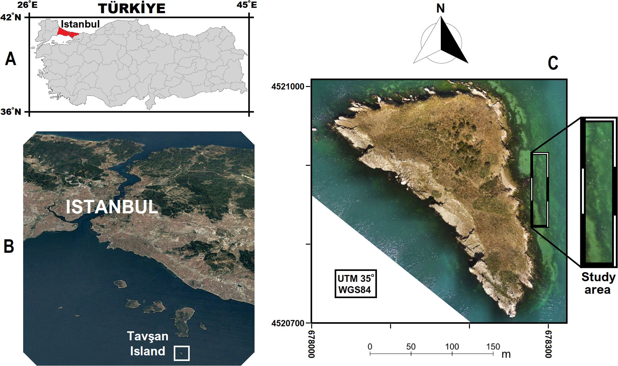
Figure 1. (A) Istanbul in Türkiye map, (B) location of Tavşan Island in Istanbul, (C) the study area on RGB orthomosaic of the Island.
The aerial photos of the Tavşan Island were captured with an average ground sampling distance (GSD; i.e., pixel size) of 3.4 cm by using DJI Phantom IV MS UAV. The UAV includes a FC6360 MS camera which have Red, Green, Blue, Red Edge, and NIR monocrome sensors and a traditional RGB sensor for visible light imaging. In addition, the UAV has a real-time kinematic (RTK) global navigation satellite system (GNSS) receiver for precise positioning. Although the UAV has an RTK receiver, ground control points (GCPs) have been established in the Island against RTK signal interruptions that frequently occur when flying over water surfaces. The GCPs were measured by utilizing a CHC i80 GNSS receiver in fixed positioning mode for the highest positioning accuracy (>3 cm). Since the MS UAV flights took 3 h–4 h, the aerial photos were affected by different lighting due to atmospheric and solar conditions; that is why radiometric calibration, converting the digital number into a unit of scene reflectance, was required (Guo et al., 2019). For radiometric calibration, MAPIR Camera Reflectance Calibration Ground Target Package V2 was employed. Table 1 shows the specifications of the used UAV, GNSS receiver, and radiometric calibration ground target.

Table 1. Specifications of used UAV, GNSS receiver, and radiometric calibration ground target.
3 Methodology
The methodology of the study consists of three main stages: i) UAV data acquisition and photogrammetric processing, ii) generation of UAV DBMs by multiple methods, and iii) accuracy assessment of UAV DBMs. These stages were presented in detail as subsections of Methodology.
3.1 UAV data acquisition and photogrammetric processing
In UAV data acquisition, many parameters should be considered for a safe flight and the generation of high-quality products. One of the most significant parameters is the flying altitude which directly affects the GSD that determines spatial resolution (Koch et al., 2019). Due to determining of the flying altitude from the UAV home point, the spatial resolution in elevated areas is higher than that of flat topography due to being closer to the UAV camera. The maximum object height in the flying path is another main parameter in flying altitude determination. In the elevated part of the Tavşan Island, two different high masts exist for safety purposes. Regarding these circumstances, two different altitude flights were planned. While the 80-m flying altitude was preferred for elevated parts of the Island, 60 m was applied for low parts and 633 aerial photos with average 3.4 cm GSD were achieved. To obtain maximum shallow water coverage and high-performance 3D modeling, different geometry polygonal flying paths with nadir view were applied in the flights.
The workflow used up to very high-resolution (VHR) orthomosaic generation with acquired MS UAV data is shown in Figure 2. Photogrammetric processing steps were completed utilizing Agisoft Metashape, one of the most preferred UAV data processing software in scientific applications. Similar to popular UAV data processing software such as Pix4D, ContextCapture, and Visual-SfM, Agisoft Metashape uses the low-cost and robust structure from motion (SfM) technique for high-resolution image matching and generation of 3D geometry from a series of overlapping aerial photos (Westoby et al., 2012). One of the main objectives of this study is to determine the effect of different imaging bands on bathymetric model quality; that is why the orthomosaic generation process was applied two times as for RGB single bands and the R, G, B, red edge, and NIR multi-bands separately. In the RGB band workflow, distinct from the MS workflow, radiometric calibration is not included because of single band usage.
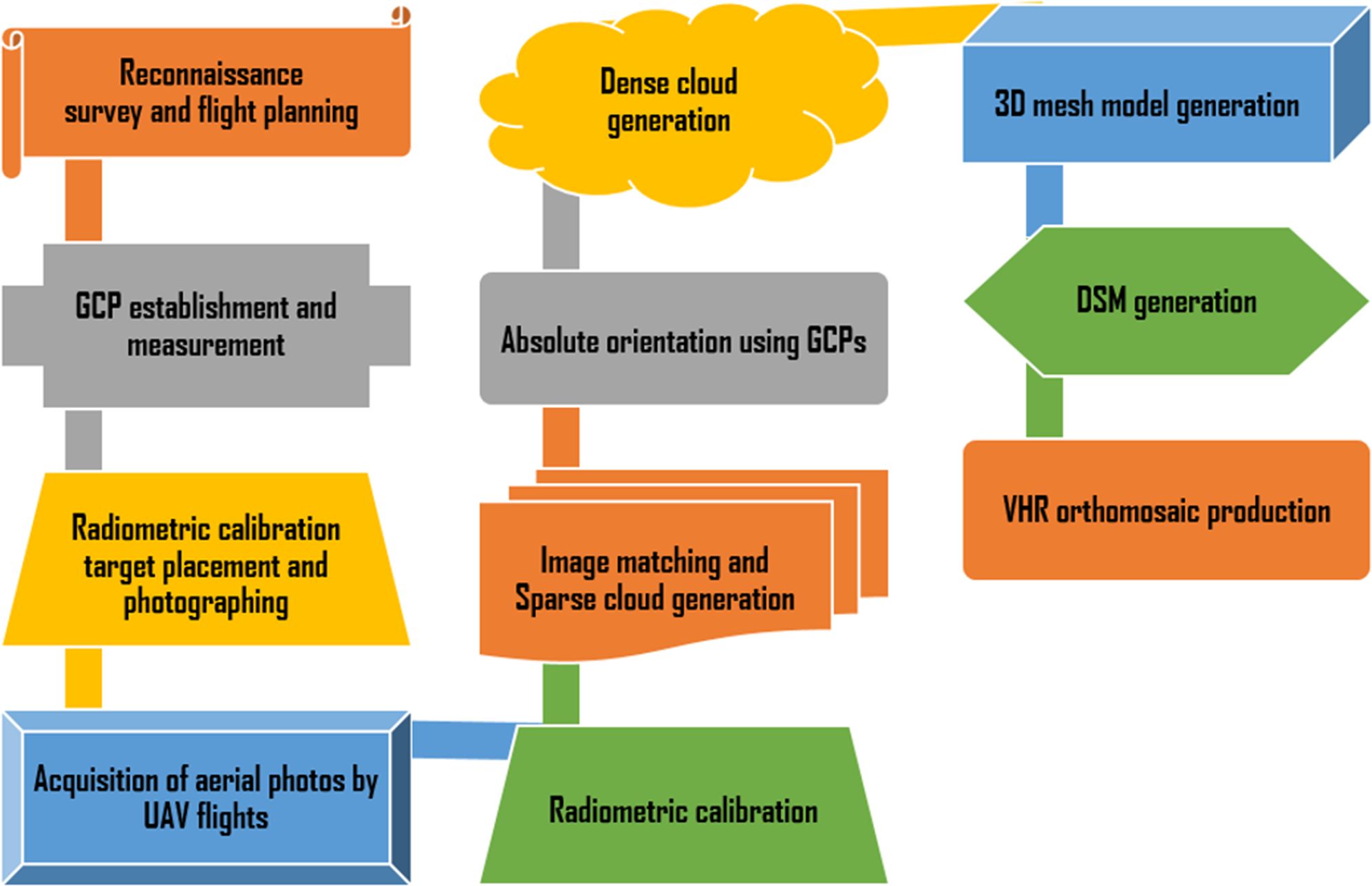
Figure 2. Workflow used up to orthomosaic generation with acquired MS UAV data.
For correct validation, raw imagery derived from remote sensing platforms has to be calibrated before scientific analyses (Lee et al., 2004). In this study, the calibration of the aerial photos was completed in two steps as radiometric and geometric. While geometric calibration is sufficient for RGB data, radiometric calibration is additionally mandatory for MS data to achieve more accurate spectral reflectance data (Teixeira et al., 2020). To use in radiometric calibration, before the flights, the photos of MAPIR Camera Reflectance Calibration Ground Target Package V2 were captured by MS UAV. In these photos, four colors placed on MAPIR V2 as white, black, light gray, and dark gray were masked separately to isolate them from the rest for a correct calibration (Sefercik et al., 2023a). The exact spectral reflectance values of these colors were obtained from the distributor of MAPIR. The geometric calibration of the aerial photos was realized in two steps as initial (mutual) alignment and absolute orientation. In initial alignment, aerial photos were matched by applying the SfM approach and sparse point clouds were generated. For absolute orientation, 13 GCPs distributed on the Island before the flight were used. In addition, 16 and 4 tie points were manually marked around the sea surface for RGB and MS data, respectively, to include aerial photos on the sea area to the orientation. The precision of GCPs and additional tie points was determined as RMSE utilizing Equation 1 where i, Ŷi, i = estimated values for i camera position and Xi, Yi, Zi = input values for i camera position.
The accuracy of the model after absolute orientation was calculated employing 5 of 13 GCPs as independent check points (ICPs). Unlike GCPs, ICPs are not used for absolute orientation and determine the 3D accuracy of the geometrically calibrated model by calculating the difference from reference GNSS measurements (Sefercik and Nazar, 2023b). The accuracies of the models acquired by oriented photos regarding ICPs were calculated by Equations 2–5. Figure 3 illustrates the masked reflectance targets and GCP distribution on the Tavşan Island. RMSE values of GCPs, additional tie points, and ICPs for MS and RGB data geometric calibration are separately presented in Table 2. Table 2 shows that the average RMSE of ICPs is approximately ±5 cm for both MS and RGB models; this means ±1.5 pixels (i.e., 5 cm/3.4 cm) and is quite sufficient considering the steep and irregular topography of the island.
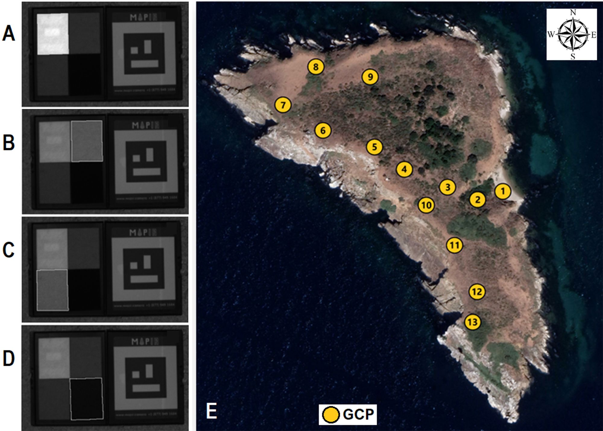
Figure 3. Masked reflectance targets: (A) white, (B) light gray, (C) dark gray and (D) black Workflow, and (E) used GCPs.
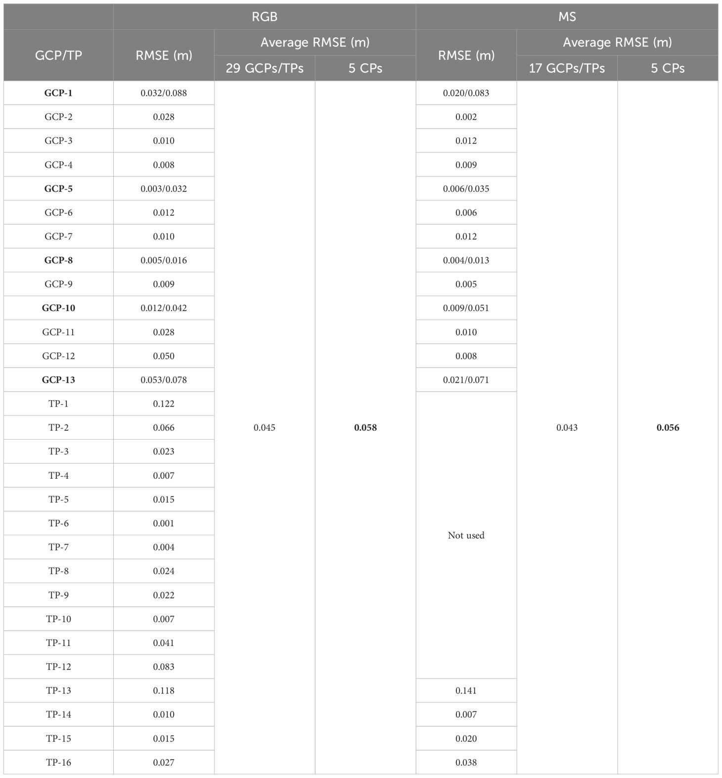
Table 2. RMSE values of GCPs, additional tie points, and ICPs for MS and RGB data geometric calibration (ICPs are dark).
Following geometric calibration processes, dense point clouds were generated for RGB and MS data using mild depth filtering, which reduces noisy points while preserving fine details. Depth filtering evaluates pairwise depth maps for matching aerial photos using the component filter, taking into account the pixel ranges from the sensor (Tinkham and Swayze, 2021). In dense point cloud of water-included study areas, when sunlight is reflected from the sea surface at the same angle as the UAV sensor views, sunlight occurs and causes considerable noise. Additionally, the reduction of image matching quality depending on low correlation of aerial photos in water areas causes noise. Therefore, generated RGB and MS dense point clouds were filtered by fencing and classifying noisy points. For the refraction correction of RGB and MS dense point clouds, an iterative approach proposed by Dietrich (2017), based on the calculation of a set of equations to correct the refraction of point/camera combinations in the point cloud, was used and it is available from a GitHub repository (https://github.com/geojames/pyBathySfM). In this approach, based on Snell’s law (Equation 6), which governs the refraction of light between two different mediums, a set of equations is solved for the actual depth h of the seafloor point.
In Equation 6, while the refractive index of seawater is 1.337 (Harvey et al., 1998) and the refractive index of air is 1.0, the incidence angle from the seabed to the water surface is and the refraction angle from the water surface to the optical sensor is . As light rays pass through the air/water interface, they are refracted according to the Snel/Descartes law of refraction, so as the camera moves, the and angles also fluctuate, affecting the values (Westaway et al., 2001; Butler et al., 2002). Hence, there is a need to solve Equation 6 for each camera position. This can be simplified to Equation 7, where represents the horizontal distance from the air/water interface to the underwater point, and is the apparent depth.
The initial step involved selecting all cameras associated with visible points within the study area. The estimated camera positions (x, y, z), orientations (pitch, roll, yaw), and internal parameters (focal length and sensor size) were then used to calculate the instantaneous field of view (IFOV) for each camera. Angles and were calculated according to Equation 8 for every visible point within the IFOV. Here, represents the Euclidean distance between the optical sensor and the underwater point and represents the vertical distance between the optical sensor and the underwater point .
Estimating a planar water surface is crucial for obtaining water surface elevations to establish . The water depth in the area can be measured, and water edge points can be sampled in the SfM point cloud to achieve this. In both RGB and MS point clouds, water edge points are selected based on the noticeable color shift from wet to dry points. For each combination of point/camera, the calculation of is carried out using the aforementioned equations and the formula for the value (Equation 9).
Finally, the true Z-coordinate of the underwater point can be calculated using Equation 10. Since is a certain value, is also certain for each point, resulting in different and values for each camera. As a result, the values of and will vary, resulting in the final corrected depth being the average of all values , explained in Butler et al. (2002) as the depth correction value calculated for each camera position and the average of these values are used to determine the , which is then subtracted from the surface of the water to obtain the corrected height.
Dense point cloud consists of non-continuous point-based vector form; for more realistic and continuous raster form, it has to be converted into the 3D solid form. That is why, using the refraction-corrected dense point clouds, 3D mesh models and digital surface models (DSMs) were generated and finally 3.42-cm GSD RGB and 3.39-cm GSD MS orthomosaics were produced (Figure 4). To demonstrate the effect of radiometric calibration, MS orthomosaics were presented with and without radiometric calibration separately in Figure 4.
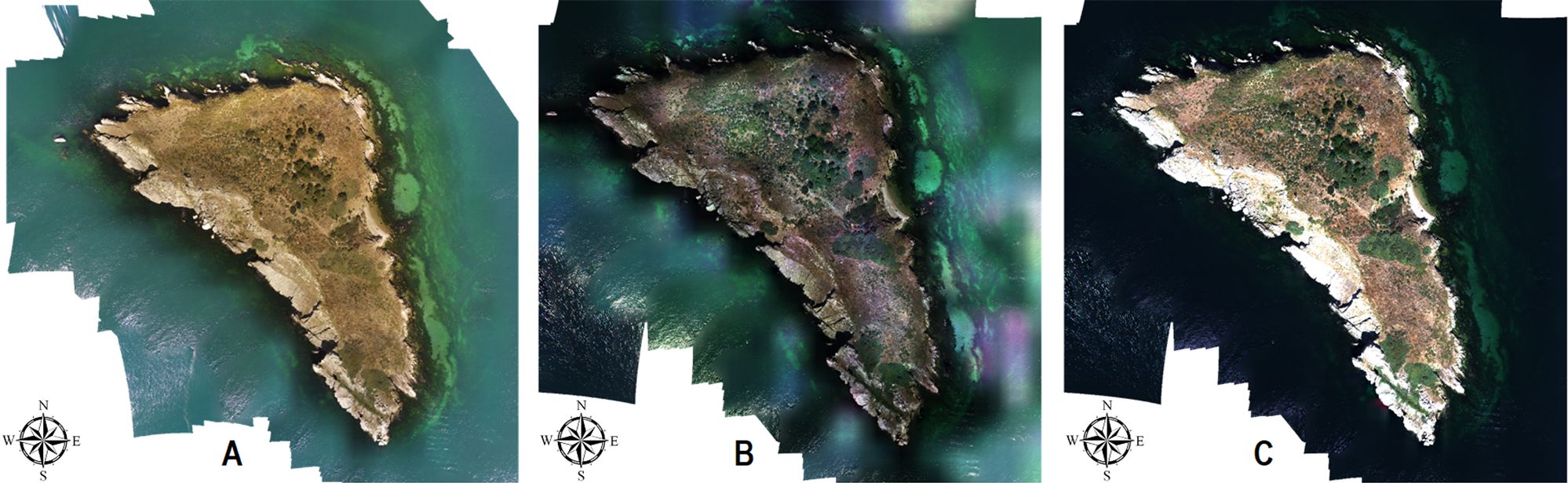
Figure 4. Generated Orthomosaics: (A) RGB, (B) MS without radiometric calibration, (C) MS with radiometric calibration.
3.2 Generation of UAV DBMs by multiple methods
In the study, four DBMs with different characteristics were generated to evaluate the effect of spectral bands and different principle generation methods on UAV-derived DBM potential in shallow water. While RGB and MS DBMs were generated from 3D dense point clouds derived by RGB and MS calibrated aerial photos, in Stumpf and Lyzenga DBM production, reflectance values of 2D MS orthomosaic were employed. The high-quality RGB and MS DBMs were generated in Surfer software using reprocessed dense point clouds in MicroStation Terrasolid, which presents more detailed point filtering advantage in comparison with Agisoft Metashape. For the generation of DBMs by Stumpf and Lyzenga empirical methods, the following methodologic workflow presented in Figure 5 was applied on MS UAV orthomosaic utilizing the ENVI™ 5.6 suite and QGIS 3.23.3 for the determination of model parameters and LibreOffice for error calculations. In preprocessing, the study area was subset and the MS orthomosaic was downsampled to 10-cm grid to generate 10-cm Stumpf and Lyzenga DBMs for 100% pixel-based overlap with the reference DBM and better interpretation with RGB and MS DBMs.

Figure 5. Generation methodology of Stumpf and Lyzenga empirical UDB DBMs.
Proper use of water pixels requires masking out any pixel containing land features including soil, vegetation, rocks, and urban. For this purpose, water pixels were extracted from the MS UAV orthomosaic by generating a land mask. This was accomplished through the normalized difference water index (NDWI) presented by McFeeters (1996) to delineate features of open water and improve their visibility in remotely sensed imagery by adopting a band ratio of green and NIR bands (Equation 11). This index is created firstly for maximizing the reflectance of water features by means of green wavelength; secondly to minimize the low reflectance values of the NIR band being absorbed mostly by water features; and thirdly to benefit from the high reflectance of vegetation and soil features in NIR band (Xu, 2006). In Equation 11, ρ_Green is the reflectance value of green band pixels and ρ_NIR is the reflectance value of NIR band pixels. Results of NDWI displayed that index values of water features were mostly larger than 0.5 similar to Du et al. (2016). Therefore, this value was selected as a threshold for water–land separability and a land mask was generated.
Indeed, Stumpf and Lyzenga are two different empirical SDB methods which are conventionally applied to satellite imagery in the literature. In this study, we adapted these methods to UAV-derived DBM generation, that is why these models will be called UDB models. An empirical solution was proposed by Stumpf et al. (2003) based on ratio transform for producing SDB models over shallow waters. This solution follows the fundamental that water absorptivity differentiates from band to band and as the depth increases, the spectral irradiance decreases at a higher rate in the higher absorption band (green band) compared with the lower absorption band (blue band) (El-Sayed, 2018). It uses the natural logarithmic ratio of two different visible bands with dissimilar absorptivities for derivating the depth value over different bottom types, and it can be applied to low-albedo depth features as an alternative to the linear transform approach (Equation 12). In addition, the ratio transform algorithm makes utilization of two bands to reduce the number of depth retrieval parameters and it can minimize errors due to differing variations in the atmosphere, water column, and sea bottom (Pushparaj and Hegde, 2017).
In the equation, is the calculated depth value, is a changeable constant to scale the ratio to depth, is a fixed constant for all zones, for the depth of 0 m is the offset, and whereas is the reflectance values of high absorption band defines the reflectance values of the low absorption band. However, to properly apply the Stumpf UDB model to MS UAV data, the most suitable band combination should be determined. This was carried out by using optimal band ratio analysis (OBRA), and wavelength pairs that establish the strongest relationship linearly between and the remotely sensed variable were analyzed (Legleiter et al., 2009). In addition, OBRA utilizes a log-ratio of bands so it aids in the selection of bands that are less sensitive to substrate variability of sea bottom (Dierssen et al., 2003; Niroumand-Jadidi and Vitti, 2016). In Equation 13, is calculated by applying log-ratio to selected bands and reflectance values. Two-by-two band pair combinations were evaluated by conducting linear regression between and flow depth. In this evaluation, single-beam echosounder reference bathymetry values to be selected as the optimal pair which has the highest correlation coefficient ( (Figure 6).
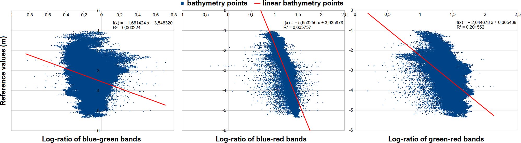
Figure 6. OBRA two-by-two band pair combinations.
values of each two-by-two band pair were obtained as 0.060224, 0.635757, and 0.201552 for blue–green, blue–red, and green–red, respectively. After carrying out OBRA using bands of MS orthomosaic, having the highest compared with other band combinations and were selected as the and , respectively, to establish a log-band ratio. In this step, to ensure that logarithms will be positive in any situation and to eliminate any non-linear response from depth, fixed constant was selected as 1,000 which is conventionally utilized in literature (Bramante et al., 2013; Caballero and Stumpf, 2020, 2023). The model parameters and were determined by applying a linear regression between the logarithmic band ratio and the single-beam echosounder reference bathymetry values as shown in Figure 7 (Zhu et al., 2020). By applying a linear regression, the trend line equation and were obtained (Equation 14).
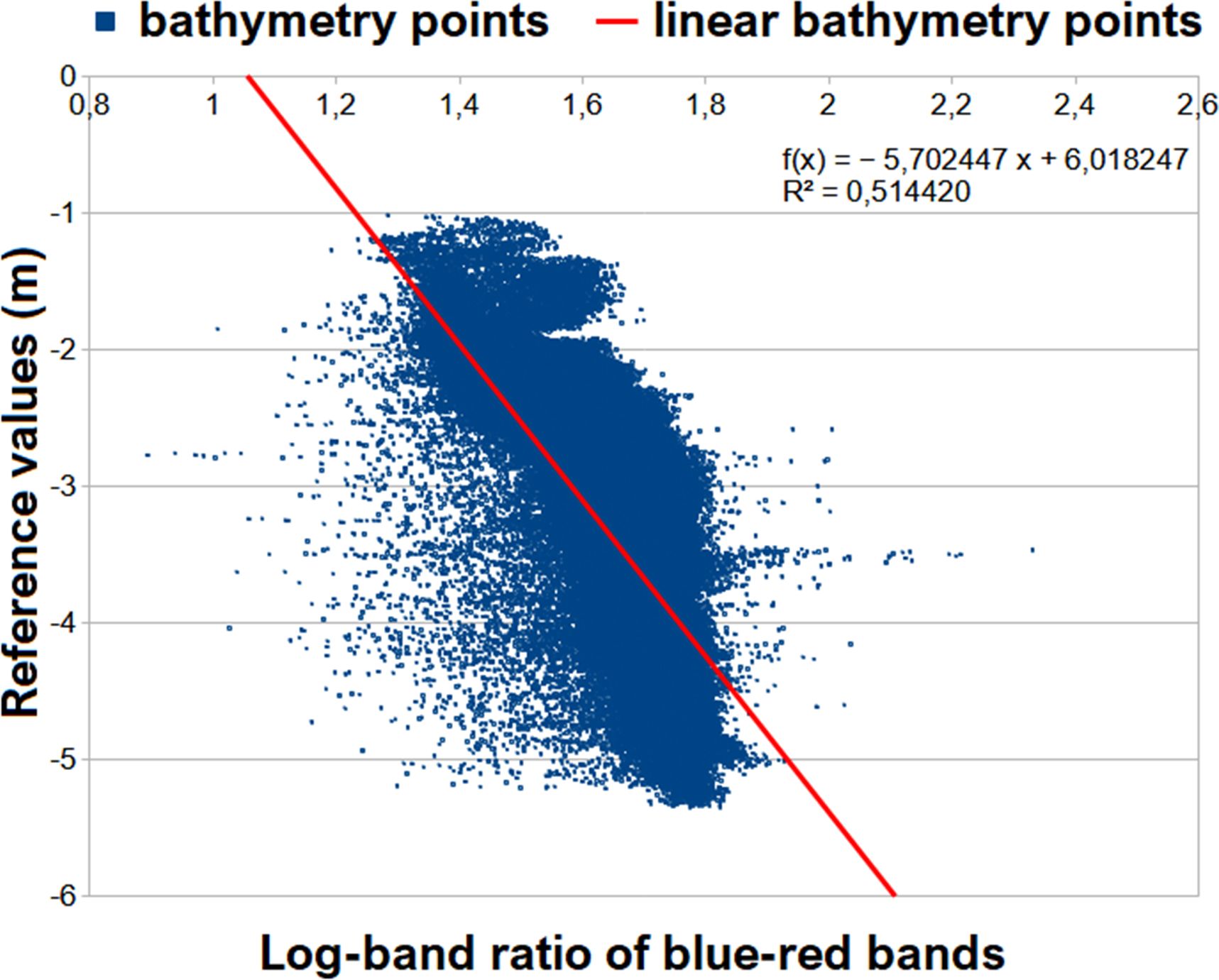
Figure 7. Linear regression between the log-band ratio and the reference values for determination of the model parameters m0 and m1.
As mentioned before, the possibility of generating UDB models from MS aerial photos was further analyzed by adopting another empirical method Lyzenga (1978), based on log-linear inversion of MS bands with advantages of i) enhanced operational flexibility due to spectral bands not restricted to the ones with the same coefficients of water attenuation, ii) enhanced performance in separation of bottom substances with similar spectral behavior, and iii) utilization of more than two bands in contrast to log-ratio based methods providing increased robustness. This method assumes that the optical properties of a water area are uniform over a sample region and reflectance values obtained from MS bands can be combined to acquire information about water attenuation (Lyzenga, 1981). However, Lyzenga et al. (2006) stated that whereas in some cases the atmospheric scattering and optical properties of water are amply uniform, in general, there may be pixel-to-pixel variations due to sunlight effect, haze, or fluctuations in water quality. The Lyzenga UDB model operates upon the fact that the reflected values from the sea floor can be approximated by using bottom reflectance values to form a linear function and utilizing water depths to produce an exponential function (Equation 15). In other words, single-beam echosounder reference bathymetry values are used to calibrate the parameters of the Lyzenga UDB model to estimate unknown depth values (Figueiredo et al., 2015).
where is the calculated depth values in meters, and are model parameters calculated for MS bands, and and are the spectral reflectance and the deep-water reflectance for MS band, respectively. Model parameters were calculated for ( = 1,2,3) spectral bands as blue, green, and red by doing multiple linear regression between logarithmic band values and single-beam echosounder reference bathymetry values (Figure 8). After multiple linear regression, Lyzenga UDB model parameters and were obtained using Equation 16.
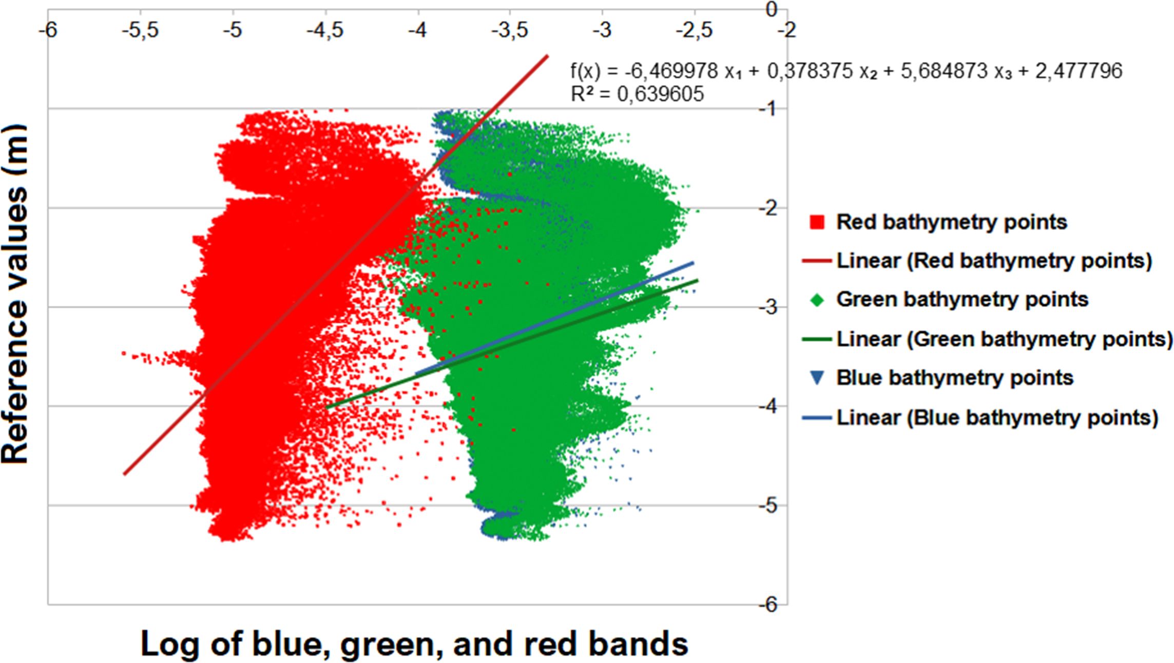
Figure 8. Multiple linear regression between the logarithmic band values and the reference values for determination of the model parameters m0 and mi.
Noise effects, especially those caused by sunlight, on Stumpf and Lyzenga DBMs were filtered using MicroStation Terrasolid software to avoid misleading results in accuracy analyses. Figure 9 shows the linear regression results of Stumpf and Lyzenga DBM values after final filtering. Considering Figure 9, it can be mentioned that Lyzenga DBM estimates the depth values better than Stumpf DBM. The value is calculated as 0.814660 for Lyzenga whereas 0.612081 for Stumpf, which demonstrates that in-depth estimation via UDB adopting more than spectral bands can improve the performance in comparison with band ratio approach.
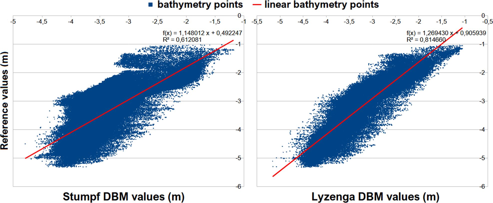
Figure 9. The linear regression of Stumpf and Lyzenga DBM values after final filtering.
3.3 Accuracy assessment of UAV DBMs
Accuracy of DBMs is assessed with two common approaches as point-based and model-based similar to other digital 3D models like digital surface, elevation, terrain, and canopy height models. While the point-based approach uses limited number of control points distributed on the study area, the model-based approach utilizes reference models. The advantage of the model-based approach is that it enables all pixels of the DBM to participate in the accuracy evaluation by comparing matching pixels in the reference 3D model (Lin et al., 1994). In this study, the model-based approach was adopted by using a reference DBM derived from single-beam echosounder measurements and all pixels of the generated DBMs were included in the accuracy analyses. In reference data acquisition, a Navisound NS 600 RT-1 single-beam echosounder, equipped with a two-channel 50-kHz transducer and a GNSS receiver, was employed. The device can reach the depth of 600 m with 1° beam width (Celik et al., 2023). As known, sonar ships generally cannot safely navigate in shallow areas. Considering this situation, a small boat, which could easily approach the island shores, was used for single-beam sonar data collection. Both the year of UAV flights and the reference single-beam echosounder data collection is 2023.
In the accuracy assessment of generated DBMs, comprehensive visual and statistical approaches were performed. In visual approaches, DBMs, and the differential DBMs (DIFFDBM) (Equation 17) which are the height error maps between generated DBMs and the reference DBM, were generated by utilizing Surfer and LISA software and interpreted. In statistical approaches, the accuracies of the generated DBMs were calculated using the standard deviation (SZ) of the height differences between the DBMs and the reference model, as well as the normalized median absolute deviation (NMAD), obtained by normalization of the median absolute deviation (Equations 18–20). The linear errors with 90% or 95% probability levels (LE90 and LE95, respectively) were not preferred as accuracy metrics because they are strongly depending on the percentage of blunders and they do not match with the frequency distribution of the height differences in most cases (Sefercik et al., 2013; Jacobsen, 2014). The statistical analyses were completed utilizing BLUH software from Leibniz University Hannover.
where is the total pixel number of generated DBMs; is the height differences from reference DBM and is the arithmetic mean of the (bias). is the median of univariate dataset (, , , …., ) and is the median of absolute values of the dataset from . In normal distribution, the values of SZ and NMAD are expected as similar. However, a qualified 3D model generation with optical remote sensing in underwater conditions is not as simple as surface conditions and in many cases large outliers are likely to arise. In that case, NMAD is used as a robust scale estimator to estimate the scale of the distribution and can be considered as an estimate for the standard deviation more resilient to outliers in the dataset (Höhle and Höhle, 2009).
To estimate the relative accuracy level between neighboring pixels on produced DBMs, contour maps of the evaluated DBMs were created and relative standard deviation (RSZ) was calculated for each pixel using 10 pixel diameter (point spacing × 10) distance groups () by Equation 21. In the equation, and are the lower and upper ranges of the group and and are closely neighbored pixels. For each pixel in distance group, the height difference from the reference DBM is considered. In Equation 21, is the number of point combinations in the distance group. To normalize RSZ to SZ, a multiplication factor of 2 for was employed. If the height differences of the neighbored points are independent as a result of error propagation, the RSZ would be the square root of larger than SZ, described by × .
To consider at the interpretations of visual and statistical approaches, Secchi Disc measurements (Zielinski, 2021) were completed around the study area and turbidity depth of the water was determined as 7.4 m. In addition, geoid undulation in the study area was calculated and applied as 36.501 m in the analyses.
4 Results and discussion
As aforementioned, four different DBMs as RGB, MS, Stumpf, and Lyzenga were generated and comprehensively evaluated by visual and statistical approaches utilizing a reference DBM produced from single-beam echosounder data. Figure 10 shows the generated reference DBM and four evaluated DBMs of the study area. According to the reference DBM, the elevation of deep topography is maximum and minimum in the Southwestern and Northeastern sides of the study area, respectively and around −1 m to −5.5 m. In the first view, the bathymetric surface descriptions of RGB and MS DBMs are closer to the reference than Stumpf and Lyzenga DBMs. In fact, the height scale of the MS DBM produced from five-band aerial photos is almost in the same range as the reference. However, the minimum elevation of RGB DBM is around −4.8 m whereas the reference is around −5.5 m. This shows that the limitations of RGB DBM increase as water depth increases. A similar situation exists for Stumpf DBM, which could not identify topographic details lower than ~−4.8 m.
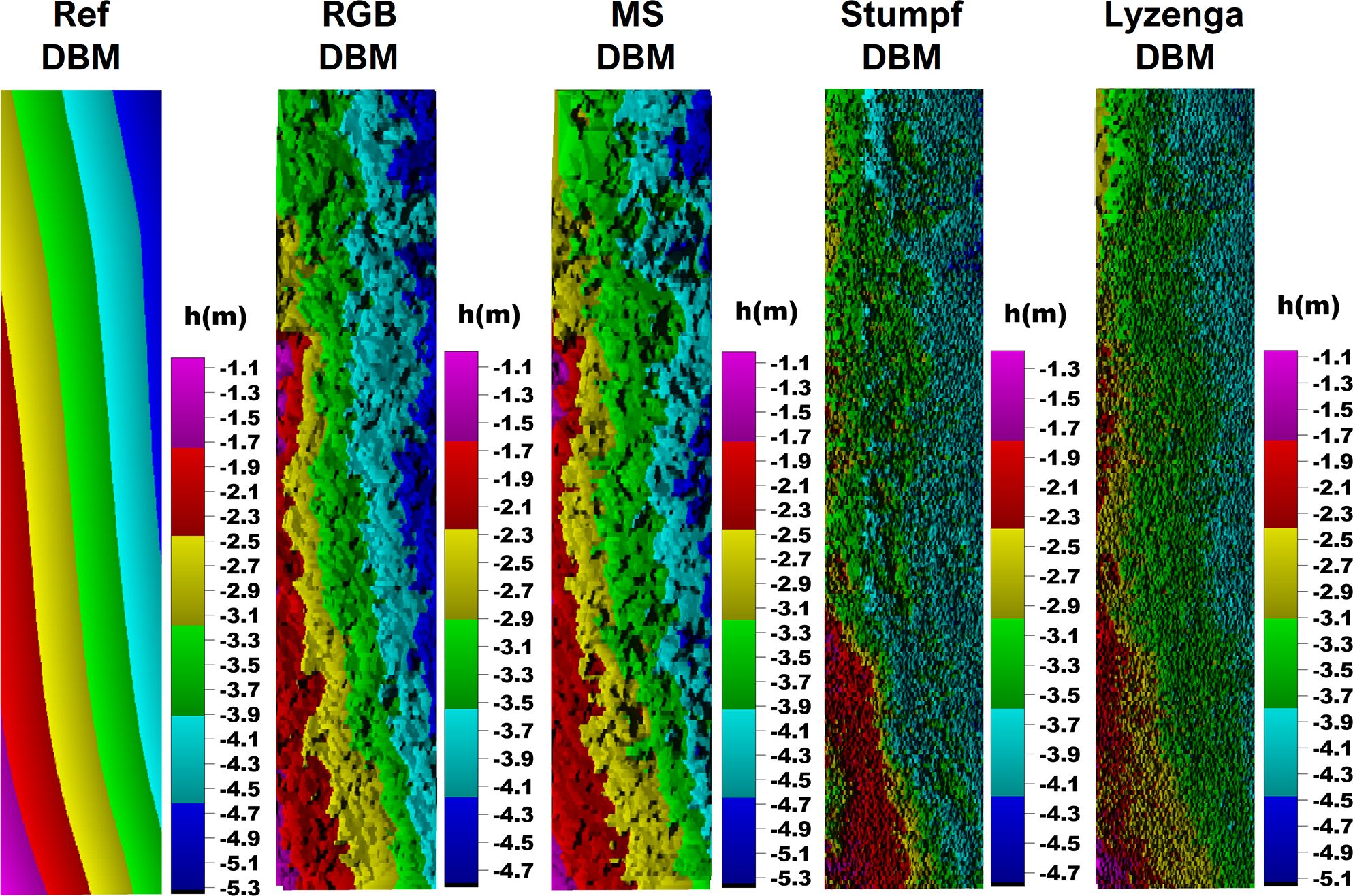
Figure 10. Generated RGB, MS, Stumpf, and Lyzenga DBMs.
The model-based absolute vertical accuracy assessment results of the generated DBMs are presented in Table 3. The systematic bias values were calculated and eliminated before the assessment, and SZ and NMAD values do not include bias. The systematic biases were determined as −0.09 m and 0.07 m for RGB and MS DBMs, respectively. As can be seen in Table 3, while the accuracies of RGB and MS DBMs based on SZ and NMAD are around ±0.23–0.27 m, they are around ±0.40–0.55 m for Stumpf and Lyzenga DBMs. This result demonstrates that generation of DBMs directly from 3D dense point clouds of the aerial photos is more reasonable than generation of DBMs using the reflectance values of the MS UAV orthomosaic. In parallel with values, the accuracy of Lyzenga DBM is higher than Stumpf DBM as both SZ and NMAD. This result also reveals that in-depth estimation via UDB adopting more than spectral bands can improve the performance in comparison with the band ratio approach.
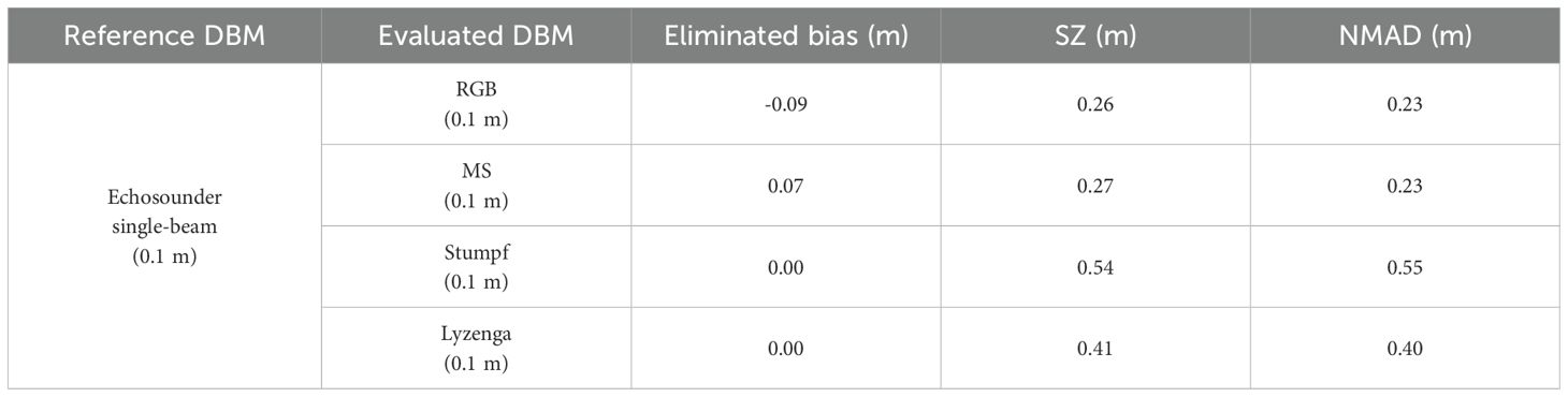
Table 3. Absolute vertical accuracies of UAV DBMs.
The frequency distribution, SZ, and NMAD of height differences between generated DBMs and the reference DBM is given by distribution graphics in Figure 11. In the graphic, while the peaks of frequency distribution of height differences (FDZ) of 3D dense point cloud-based RGB and MS UAV DBMs are around 30K pixels, it is around 15K pixels for UDB DBMs. In SZ and NMAD sides, symmetric distribution, which reveals a normal error propagation, is available for all DBMs. The NMAD distributions of RGB and MS DBMs are very similar to each other whereas SZ is slightly different. SZ and NMAD distributions prove that Lyzenga DBM performs better compared with Stumpf DBM.
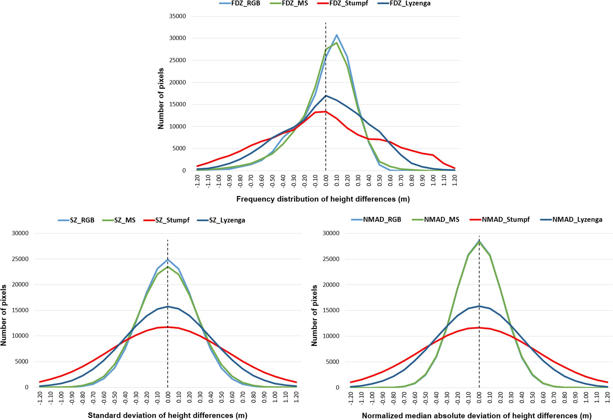
Figure 11. FDZ, SZ, and NMAD of DBM height differences from reference DBM.
Figure 12 shows the contour maps which enable to interpret relative vertical accuracies between neighboring pixels on generated DBMs. While the contour lines are clearly detectable in RGB and MS DBMs, small contour islands stand out in UDB DBMs with a discontinuous structure. This points out irregular morphologic description of the seabed. The RSZ values in Figure 13 can assist to interpret this situation. While the RSZ values of RGB and MS DBMs begin around ±0.03 m, they are around ±0.11 m for Stumpf and Lyzenga DBMs. Particularly in Stumpf DBM, the RSZ trend is sharper than expected and the values reach up to ±0.3 m. The main reason of this result may be very high resolution (0.1 m) of the UAV dataset against space-borne datasets that are commonly utilized for Stumpf and Lyzenga methods.
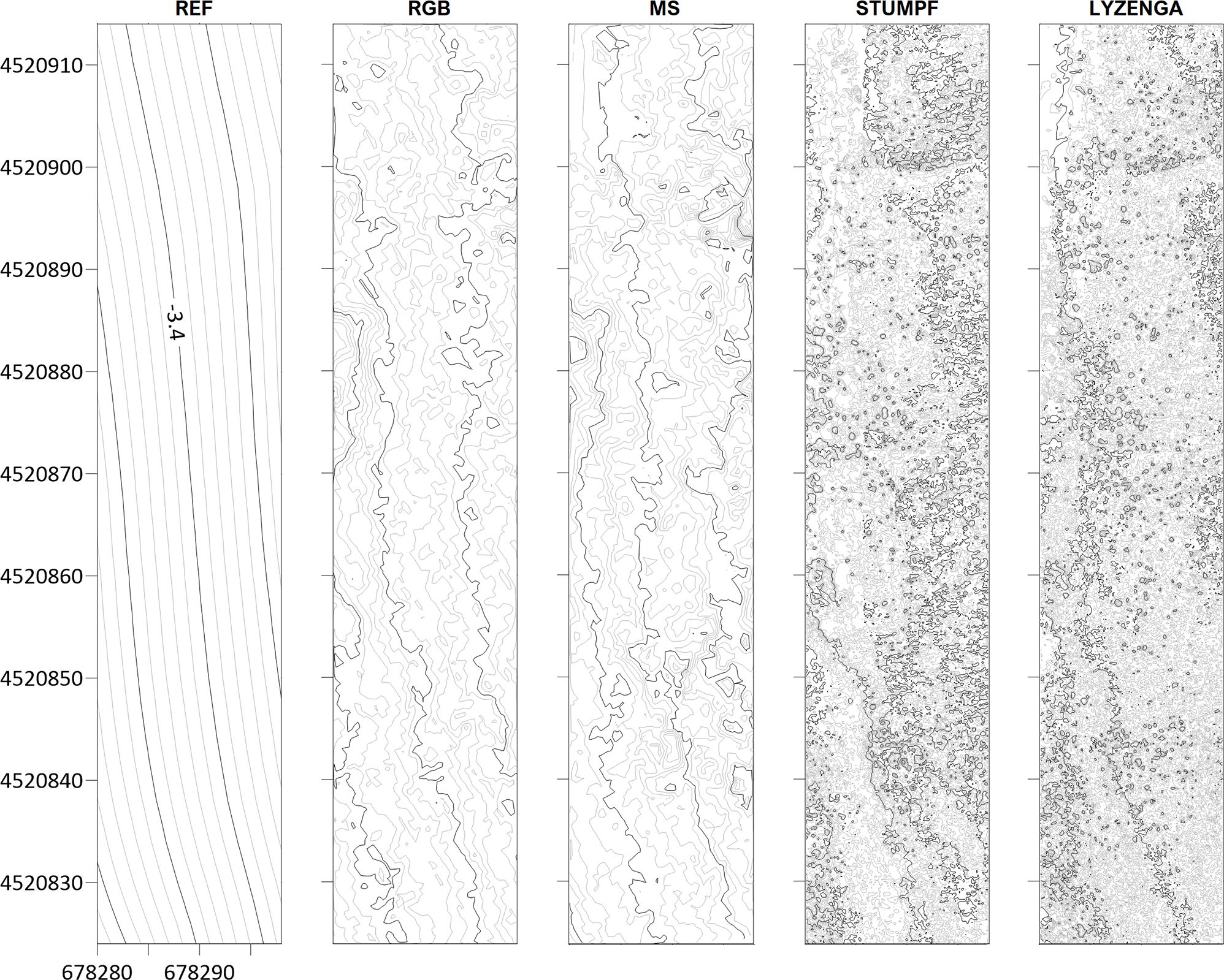
Figure 12. Morphologic structure of generated DBMs.
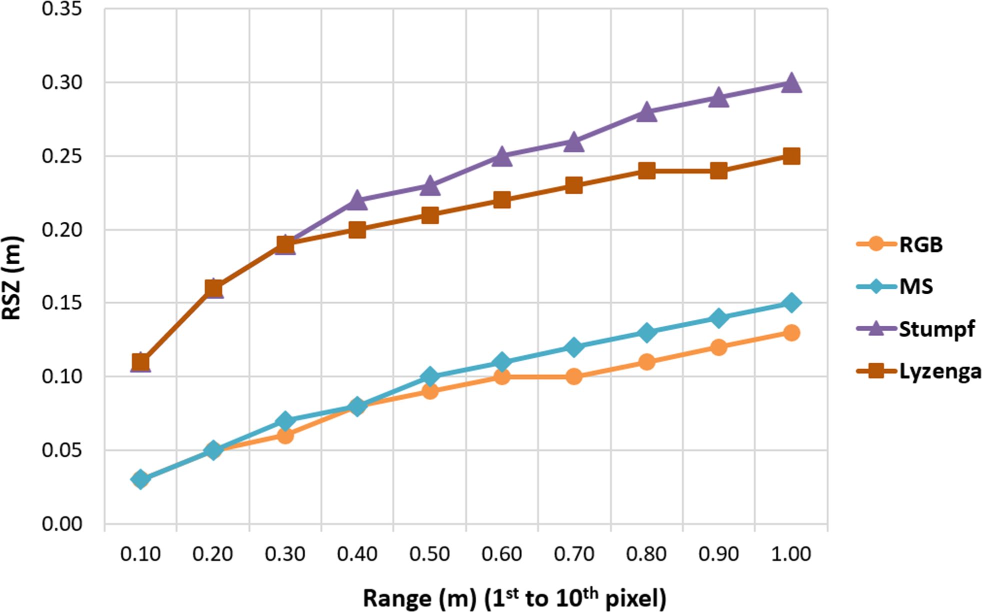
Figure 13. RSZ of generated DBMs.
The DIFFDBMs, differential DBMs of evaluated DBMs with the reference DBM, are presented in Figure 14. For better interpretation, the 3D dense point cloud-based RGB and MS DIFFDBMs and Stumpf and Lyzenga UDB DIFFDBMs were validated separately and the height differences between these validated DBMs and the reference DBMs were classified as between ±1 m, ± 0.5 m, and ±0.1 m. The dark-blue color points out that the height difference interval is exceeded. As mentioned before, water deepens from Southwest to Northeast of the study area and the first result of DIFFDBMs is that the accuracy of all analyzed DBMs decreases with increasing water depth. According to the reference DBM, the depth of the water in the study area is around −1 m and −5.5 m and considering the Secchi disc value (7.4 m), turbidity does not exist. From this point of view, it can be discussed that there is a quality limitation in all four UAV-based DBMs, although there is no turbidity in the study area. In general view, the 3D dense point cloud-based RGB and MS DBMs are more coherent with the reference and in the large part of the ±1-m DIFFDBMs, continuous structure is available without exceeding the height difference scale. There are gaps at the scales of ±0.5 m and ±0.1 m, as expected under underwater conditions.
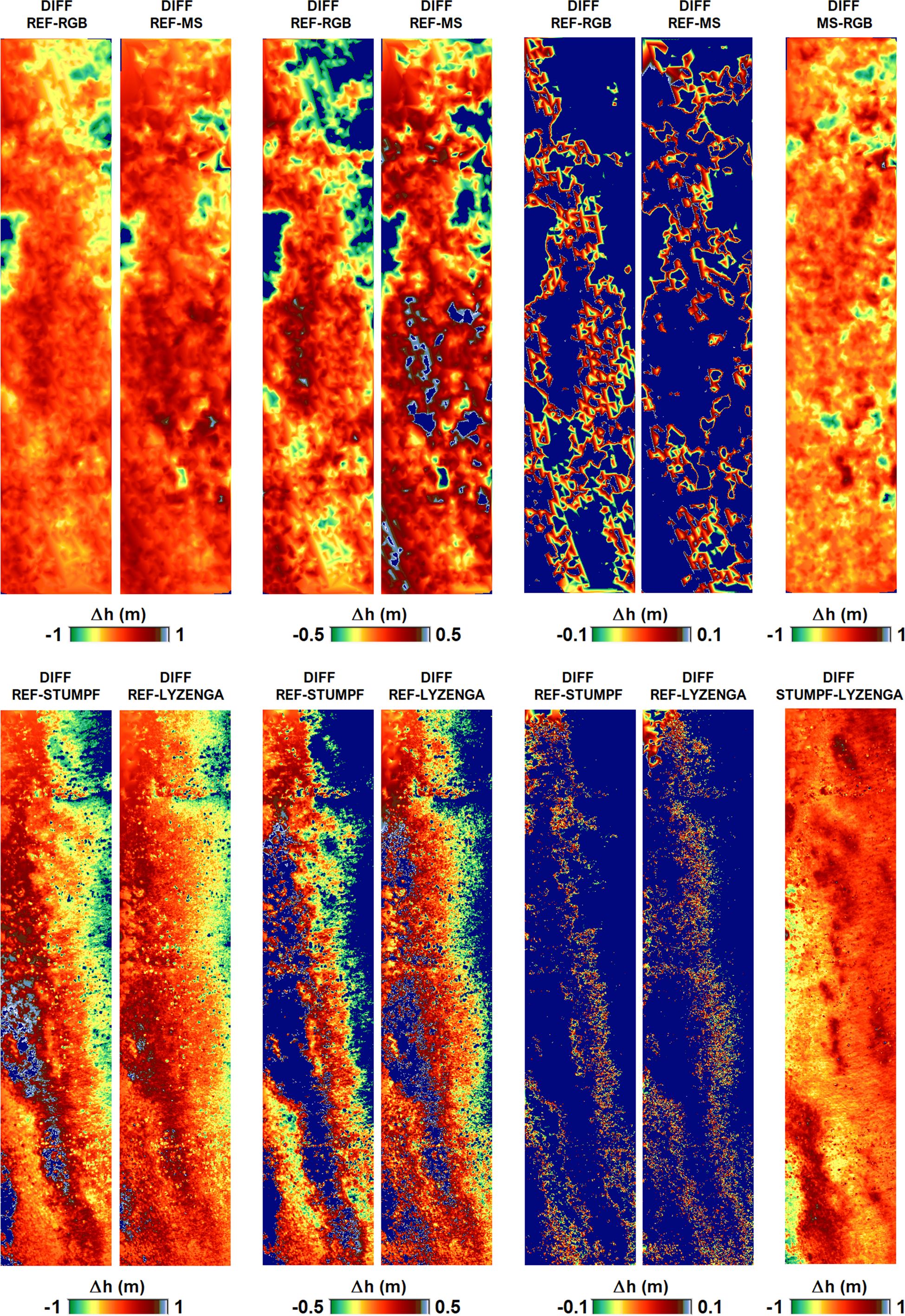
Figure 14. DIFF models of RGB, MS, Stumpf, and Lyzenga DBMs according to reference DBM.
At the ±0.1-m scale, a considerable part of MS DBM was still coherent with the reference in the deepest areas whereas RGB not. No doubt, this result demonstrates the advantage of multiband usage in UAV-based bathymetric modeling. In the UDB DBM side, it is clearly seen that Lyzenga DBM’s compatibility with the reference is much higher than Stumpf DBM in every height difference range. Additionally, the ±1-m scale DIFFDBMs of RGB-MS and Stumpf-Lyzenga DBMs are also included in Figure 14. While the consistency of RGB and MS DBMs is high at minimum and medium depths, differences of close to 1 m occur at maximum depths. Stumpf and Lyzenga DIFFDBM have an irregular distribution of height differences, and considerable differences are noticeable even at minimum depths in addition to deepest areas.
5 Conclusion
The use of UAVs in DBM generation in shallow waters is increasing permanently due to its potential to provide rapid, periodic, and very high-resolution data. However, several parameters related with sensor characteristics, imaging geometry, and calibration requirements limit the UAV-derived DBM quality. In this paper, four DBMs, two from single-band RGB and five-band MS 3D dense point clouds and Stumpf and Lyzenga UDB methods, were generated and comprehensively analyzed by visual and statistical model-based comparison approaches. Before the analyses, radiometric and geometric calibrations of UAV aerial photos were carefully completed. While 13 GCPs and 16 additional TPs were used for absolute orientation of RGB aerial photos, 13 GCPs and 4 TPs were used for MS. In both models, five similar ICPs selected from GCPs were employed and approx. ± 0.05-m general orientation accuracy were achieved. In optimal MS band combination determination to properly apply Stumpf and Lyzenga UDB models using very high-resolution MS orthomosaic, OBRA were applied and blue–red band combination was preferred accordingly. To avoid misleading depth description, refraction correction was applied in the generation of all evaluated DBMs.
While DBMs and the DIFFDBMs were generated for visual accuracy analyses, SZ and NMAD of the height differences between the DBMs and the reference model were utilized in statistical analyses. In addition to absolute vertical accuracies, the relative accuracies of the DBMs were also exposed by RSZ calculation for neighboring pixels by distance grouping and morphologic analyses by creating contour-lines. The results of visual and statistical analyses demonstrated that i) the accuracy of all analyzed DBMs decreases as water depth increases considering the DIFFDBMs and ii) the accuracy of RGB and MS DBMs produced from 3D point clouds of aerial photos is higher than DBMs produced from Stumpf and Lyzenga UDB methods. While SZ and NMAD of RGB and MS DBMs are around ±0.23 m–0.27 m, this is around ±0.40 m–0.55 m for UDB DBMs. In detailed view, the representation capability of MS DBM is higher than that of RGB DBM and that of Lyzenga DBM is higher than that of Stumpf as the water depth increases. In contrast, it has been observed that the situation reverses in minimum depths. In addition, the systematic bias determined in RGB DBM between reference DBM was determined as −0.09 m, whereas in MS, it was determined as 0.07 m. iii) Relative accuracies of RGB and MS DBMs produced from 3D point clouds are also higher than UDB DBMs. While RSZ values are between ±0.03 m and 0.15 m for RGB and MS DBMs, they are ±0.11–0.30 m for Stumpf and Lyzenga DBMs. In addition, generated contour lines revealed the noisy structure of Stumpf and Lyzenga DBMs in comparison with RGB and MS DBMs that cause small contour islands. The reason of this result may be the very high resolution (0.1 m) of the UAV dataset against space-borne datasets that are commonly utilized for Stumpf and Lyzenga methods.
Overall, the accuracy of DBMs generated with different techniques has been documented, thus allowing their use for different bathymetric purposes to be evaluated. The advantages and disadvantages of generated DBMs compared with each other are discussed. The common conclusion is that the results given by the examined DBMs can be evaluated for shallow waters up to 5-m depth. It has been documented that at depths greater than 5 m, height differences (i.e., height error) between tested and reference DBMs are partially greater than ±1 m.
Data availability statement
The raw data supporting the conclusions of this article will be made available by the authors, without undue reservation. All data used in this study is available in Gebze Technical University, Department of Geomatics Engineering and Istanbul University, Institute of Marine Science and Management.
Author contributions
US: Writing – review & editing, Writing – original draft, Visualization, Validation, Supervision, Software, Resources, Project administration, Methodology, Investigation, Funding acquisition, Formal analysis, Data curation, Conceptualization. MN: Investigation, Funding acquisition, Formal analysis, Data curation, Conceptualization, Writing – review & editing, Writing – original draft, Visualization, Validation, Supervision, Software, Resources, Project administration, Methodology. IA: Writing – review & editing, Writing – original draft, Visualization, Validation, Supervision, Software, Resources, Project administration, Methodology, Investigation, Funding acquisition, Formal analysis, Data curation, Conceptualization. GB: Writing – review & editing, Writing – original draft, Visualization, Validation, Supervision, Software, Resources, Project administration, Methodology, Investigation, Funding acquisition, Formal analysis, Data curation, Conceptualization. CG: Writing – review & editing, Writing – original draft, Visualization, Validation, Supervision, Software, Resources, Project administration, Methodology, Investigation, Funding acquisition, Formal analysis, Data curation, Conceptualization. IB: Writing – review & editing, Writing – original draft, Visualization, Validation, Supervision, Software, Resources, Project administration, Methodology, Investigation, Funding acquisition, Formal analysis, Data curation, Conceptualization.
Funding
The author(s) declare financial support was received for the research, authorship, and/or publication of this article. This research was funded by the Scientific Research Projects Coordination Unit of Istanbul University under the Research Universities Support Program with Project Number FBA-2023-39478.
Acknowledgments
The authors would like to thank Dr. Karsten Jacobsen and Dr. Wilfred Linder for providing BLUH and LISA software as free of charge.
Conflict of interest
The authors declare that the research was conducted in the absence of any commercial or financial relationships that could be construed as a potential conflict of interest.
Publisher’s note
All claims expressed in this article are solely those of the authors and do not necessarily represent those of their affiliated organizations, or those of the publisher, the editors and the reviewers. Any product that may be evaluated in this article, or claim that may be made by its manufacturer, is not guaranteed or endorsed by the publisher.
References
Agrafiotis P., Karantzalos K., Georgopoulos A., Skarlatos D. (2020). Correcting image refraction: Towards accurate aerial image-based bathymetry mapping in shallow waters. Remote Sens. 12, 322. doi: 10.3390/rs12020322
Agrafiotis P., Karantzalos K., Georgopoulos A., Skarlatos D. (2021). Learning from synthetic data: Enhancing refraction correction accuracy for airborne image-based bathymetric mapping of shallow coastal waters. PFG–Journal Photogrammetry Remote Sens. Geoinformation Sci. 89, 91–109. doi: 10.1007/s41064-021-00144-1
Agrafiotis P., Skarlatos D., Forbes T., Poullis C., Skamantzari M., Georgopoulos A. (2018). Underwater photogrammetry in very shallow waters: main challenges and caustics effect removal. Int. Arch. Photogrammetry Remote Sens. Spatial Inf. Sci. 42, 15–22. doi: 10.5194/isprs-archives-XLII-2-15-2018
Agrafiotis P., Skarlatos D., Georgopoulos A., Karantzalos K. (2019). DepthLearn: learning to correct the refraction on point clouds derived from aerial imagery for accurate dense shallow water bathymetry based on SVMs-fusion with LiDAR point clouds. Remote Sens. 11, 2225. doi: 10.3390/rs11192225
Alevizos E., Alexakis D. D. (2022a). Evaluation of radiometric calibration of drone-based imagery for improving shallow bathymetry retrieval. Remote Sens. Lett. 13, 311–321. doi: 10.1080/2150704X.2022.2030068
Alevizos E., Alexakis D. D. (2022b). Monitoring short-term morphobathymetric change of nearshore seafloor using drone-based multispectral imagery. Remote Sens. 14, 6035. doi: 10.3390/rs14236035
Alevizos E., Nicodemou V. C., Makris A., Oikonomidis I., Roussos A., Alexakis D. D. (2022a). Integration of photogrammetric and spectral techniques for advanced drone-based bathymetry retrieval using a deep learning approach. Remote Sens. 14, 4160. doi: 10.3390/rs14174160
Alevizos E., Oikonomou D., Argyriou A. V., Alexakis D. D. (2022b). Fusion of drone-based RGB and multi-spectral imagery for shallow water bathymetry inversion. Remote Sens. 14, 1127. doi: 10.3390/rs14051127
Alvarez L. V., Moreno H. A., Segales A. R., Pham T. G., Pillar-Little E. A., Chilson P. B. (2018). Merging unmanned aerial systems (UAS) imagery and echo soundings with an adaptive sampling technique for bathymetric surveys. Remote Sens. 10, 1362. doi: 10.3390/rs10091362
Apicella L., De Martino M., Ferrando I., Quarati A., Federici B. (2023). Deriving coastal shallow bathymetry from Sentinel 2-, Aircraft-and UAV-derived orthophotos: A case study in Ligurian Marinas. J. Mar. Sci. Eng. 11, 671. doi: 10.3390/jmse11030671
Belcore E., Di Pietra V. (2022). Laying the foundation for an artificial neural network for photogrammetric riverine bathymetry. Int. Arch. Photogrammetry Remote Sens. Spatial Inf. Sci. 48, 51–58. doi: 10.5194/isprs-archives-XLVIII-4-W1-2022-51-2022
Bindoff N. L., Willebrand J., Artale V., Cazenave A., Gregory J. M., Gulev S., et al. (2007). “Observations: Oceanic climate change and sea level, in Climate Change 2007: The Physical Science Basis,” in Contribution of Working Group I to the Fourth Assessment Report of the Intergovernmental Panel on Climate Change. Eds. Solomon S., Qin D., Manning M., Chen Z., Marquis M., Averyt K. B., Tignor M., Miller H. L. (Cambridge University Press, Cambridge), 385–428.
Bio A., Bastos L., Granja H., Henriques R., Madeira S., Rodrigues D. (2015). Methods for coastal monitoring and erosion risk assessment: two. Portuguese Case Stud. 15, 47–63. doi: 10.5894/rgci490
Bramante J. F., Raju D. K., Sin T. M. (2013). Multispectral derivation of bathymetry in Singapore’s shallow, turbid waters. Int. J. Remote Sens. 34, 2070–2088. doi: 10.1080/01431161.2012.734934
Butler J., Lane S., Chandler J., Porfiri E. (2002). Through-water close range digital photogrammetry in flume and field environments. Photogrammetric Rec. 17, 419–439. doi: 10.1111/0031-868X.00196
Caballero I., Stumpf R. P. (2020). Towards routine mapping of shallow bathymetry in environments with variable turbidity: Contribution of Sentinel-2A/B satellites mission. Remote Sens. 12, 451. doi: 10.3390/rs12030451
Caballero I., Stumpf R. P. (2023). Confronting turbidity, the major challenge for satellite-derived coastal bathymetry. Sci. Total Environ. 870, 161898. doi: 10.1016/j.scitotenv.2023.161898
Cai X., Wu L., Li Y., Lei S., Xu J., Lyu H., et al. (2023). Remote sensing identification of urban water pollution source types using hyperspectral data. J. Hazardous Materials 459, 132080. doi: 10.1016/j.jhazmat.2023.132080
Cao B., Fang Y., Jiang Z., Gao L., Hu H. (2019). Shallow water bathymetry from WorldView-2 stereo imagery using two-media photogrammetry. Eur. J. Remote Sens. 52, 506–521. doi: 10.1080/22797254.2019.1658542
Carbonneau P. E., Dietrich J. T. (2016). Cost-effective non-metric photogrammetry from consumer-grade sUAS: implications for direct georeferencing of structure from motion photogrammetry. Earth surface processes landforms 42, 473–486. doi: 10.1002/esp.4012
Casella E., Lewin P., Ghilardi M., Rovere A., Bejarano S. (2022). Assessing the relative accuracy of coral heights reconstructed from drones and structure from motion photogrammetry on coral reefs. Coral Reefs 41, 869–875. doi: 10.1007/s00338-022-02244-9
Celik O. I., Büyüksalih G., Gazioglu C. (2023). Improving the accuracy of satellite-derived bathymetry using multi-layer perceptron and random forest regression methods: A case study of Tavşan Island. J. Mar. Sci. Eng. 11, 2090. doi: 10.3390/jmse11112090
Celik O. I., Gazioglu C. (2022). Coast type based accuracy assessment for coastline extraction from satellite image with machine learning classifiers. Egyptian J. Remote Sens. Space Sci. 25, 289–299. doi: 10.1016/j.ejrs.2022.01.010
Colkesen I., Kavzoglu T., Sefercik U. G., Ozturk M. Y. (2023). Automated mucilage extraction index (AMEI): A novel spectral water index for identifying marine mucilage formations from Sentinel-2 imagery. Int. J. Remote Sens. 44, 105–141. doi: 10.1080/01431161.2022.2158049
De Kerf T., Gladines J., Sels S., Vanlanduit S. (2020). Oil spill detection using machine learning and infrared images. Remote Sens. 12, 4090. doi: 10.3390/rs12244090
Dierssen H. M., Zimmerman R. C., Leathers R. A., Downes T. V., Davis C. O. (2003). Ocean color remote sensing of seagrass and bathymetry in the Bahamas Banks by high-resolution airborne imagery. Limnol. Oceanogr. 48, 444–455. doi: 10.4319/lo.2003.48.1_part_2.0444
Dietrich J. T. (2017). Bathymetric structure-from-motion: Extracting shallow stream bathymetry from multi-view stereo photogrammetry. Earth Surface Processes Landforms 42, 355–364. doi: 10.1002/esp.4060
Doukari M., Katsanevakis S., Soulakellis N., Topouzelis K. (2021). The effect of environmental conditions on the quality of UAS orthophoto-maps in the coastal environment. ISPRS Int. J. Geo-Information 10, 18. doi: 10.3390/ijgi10010018
Dronkers J. (2005). Dynamics of Coastal Systems. Advanced Series on Ocean Engineering Vol. 25 (Hackensack: World Scientific Publishing Company), 519. doi: 10.1142/ASOE
Du Y., Zhang Y., Ling F., Wang Q., Li W., Li X. (2016). Water bodies’ mapping from Sentinel-2 imagery with modified normalized difference water index at 10-m spatial resolution produced by sharpening the SWIR band. Remote Sens. 8, 354. doi: 10.3390/rs8040354
El-Sayed M. S. (2018). Comparative study of satellite images performance in mapping lake bathymetry: Case study of Al-Manzala Lake, Egypt. Am. J. Geographic Inf. System 7, 82–87. doi: 10.5923/j.ajgis.20180703.02
Figueiredo I. N., Pinto L., Goncalves G. (2015). A modified Lyzenga’s model for multispectral bathymetry using Tikhonov regulariza-tion. IEEE Geosci. Remote Sens. Lett. 13, 53–57. doi: 10.1109/LGRS.2015.2496401
Gao B. C., Montes M. J., Li R. R., Dierssen H. M., Davis C. O. (2007). An atmospheric correction algorithm for remote sensing of bright coastal waters using MODIS land and ocean channels in the solar spectral region. IEEE Trans. Geosci. Remote Sens. 45, 1835–1843. doi: 10.1109/TGRS.2007.895949
Guo Y., Senthilnath J., Wu W., Zhang X., Zeng Z., Huang H. (2019). Radiometric calibration for multispectral camera of different imaging conditions mounted on a UAV platform. Sustainability 11, 978. doi: 10.3390/su11040978
Halpern B. S., Walbridge S., Selkoe K. A., Kappel C. V., Micheli F., d’Agrosa C., et al. (2008). A global map of human impact on marine ecosystems. Science 319, 948–952. doi: 10.1126/science.1149345
Harvey A. H., Gallagher J. S., Sengers J. L. (1998). Revised formulation for the refractive index of water and steam as a function of wavelength, temperature and density. J. Phys. Chem. Ref. Data 27, 761–774. doi: 10.1063/1.556029
He J., Lin J., Liao X. (2022). Fully-covered bathymetry of clear tufa lakes using UAV-acquired overlapping images and neural networks. J. Hydrol. 615, 128666. doi: 10.1016/j.jhydrol.2022.128666
Höhle J., Höhle M. (2009). Accuracy assessment of digital elevation models by means of robust statistical methods. ISPRS J. Photogrammetry Remote Sens. 64, 398–406. doi: 10.1016/j.isprsjprs.2009.02.003
Isgró M. A., Basallote M. D., Barbero L. (2022). Unmanned aerial system-based multispectral water quality monitoring in the Iberian Pyrite Belt (SW Spain). Mine Water Environ. 41, 30–41. doi: 10.1007/s10230-021-00837-4
Jacobsen K. (2014). Development of large area covering height model. Int. Arch. Photogrammetry Remote Sens. Spatial Inf. Sci. XL-4 40, 105–110. doi: 10.5194/isprsarchives-XL-4-105-2014
Jagalingam P., Akshaya B. J., Hegde A. V. (2015). Bathymetry mapping using Landsat 8 satellite imagery. Proc. Eng. 116, 560–566. doi: 10.1016/j.proeng.2015.08.326
James M. R., Robson S. (2014). Mitigating systematic error in topographic models derived from UAV and ground-based image networks. Earth Surface Processes Landforms 39, 1413–1420. doi: 10.1002/esp.3609
Jégat V., Pe’eri S., Freire R., Klemm A., Nyberg J. (2016). “Satellite-derived bathymetry: Performance and production,” in Proceedings of the Canadian Hydrographic ConferenceHalifax, NS, Canada. 16–19.
Kavzoglu T., Colkesen I., Sefercik U. G., Ozturk M. Y. (2021). Detection and analysis of marine mucilage bloom in the Sea of Marmara by a machine learning algorithm from multi-temporal optical and thermal satellite images. Mapp. J. 166, 1–9.
Kim S. Y., Kwon D. Y., Jang A., Ju Y. K., Lee J. S., Hong S. (2023). A review of UAV integration in forensic civil engineering: From sensor technologies to geotechnical, structural and water infrastructure applications. Measurement 224, 113886. doi: 10.1016/j.measurement.2023.113886
Koch T., Körner M., Fraundorfer F. (2019). Automatic and semantically-aware 3D UAV flight planning for image-based 3D reconstruction. Remote Sens. 11, 1550. doi: 10.3390/rs11131550
Labuz T. A. (2015). Environmental impacts—coastal erosion and coastline changes. Second Assess. Climate Change Baltic Sea basin. Editors: Bolle H. J., Menenti M., Rasool S. I., 381–396. doi: 10.1007/978-3-319-16006-1_20
Lambert S. E., Parrish C. E. (2023). Refraction correction for spectrally derived bathymetry using UAS imagery. Remote Sens. 15, 3635. doi: 10.3390/rs15143635
Lange A. M., Fiedler J. W., Merrifield M. A., Guza R. T. (2023). UAV video-based estimates of nearshore bathymetry. Coast. Eng. 185, 104375. doi: 10.1016/j.coastaleng.2023.104375
Lee C. H., Liu L. W., Wang Y. M., Leu J. M., Chen C. L. (2022). Drone-based bathymetry modeling for mountainous shallow rivers in Taiwan using machine learning. Remote Sens. 14, 3343. doi: 10.3390/rs14143343
Lee D. S., Storey J. C., Choate M. J., Hayes R. W. (2004). Four years of Landsat-7 on-orbit geometric calibration and performance. IEEE Trans. Geosci. Remote Sens. 42, 2786–2795. doi: 10.1109/TGRS.2004.836769
Legleiter C. J., Roberts D. A., Lawrence R. L. (2009). Spectrally based remote sensing of river bathymetry. Earth Surface Processes Landforms 34, 1039–1059. doi: 10.1002/esp.1787
Lin Q., Vesecky J. F., Zebker H. A. (1994). Comparison of elevation derived from Insar data with DEM over large relief terrain. Int. J. Remote Sens. 15, 1775–1790. doi: 10.1080/01431169408954208
Lingua A. M., Maschio P., Spadaro A., Vezza P., Negro G. (2023). Iterative refraction-correction method on mvs-sfm for shallow stream bathymetry. Int. Arch. Photogrammetry Remote Sens. Spatial Inf. Sci. 48, 249–255. doi: 10.5194/isprs-archives-XLVIII-1-W1-2023-249-2023
Lubczonek J., Kazimierski W., Zaniewicz G., Lacka M. (2021). Methodology for combining data acquired by unmanned surface and aerial vehicles to create digital bathymetric models in shallow and ultra-shallow waters. Remote Sens. 14, 105. doi: 10.3390/rs14010105
Lyzenga D. R. (1978). Passive remote sensing techniques for mapping water depth and bottom features. Appl. optics 17, 379–383. doi: 10.1364/AO.17.000379
Lyzenga D. R. (1981). Remote sensing of bottom reflectance and water attenuation parameters in shallow water using aircraft and Landsat data. Int. J. Remote Sens. 2, 71–82. doi: 10.1080/01431168108948342
Lyzenga D. R., Malinas N. P., Tanis F. J. (2006). Multispectral bathymetry using a simple physically based algorithm. IEEE Trans. Geosci. Remote Sens. 44, 2251–2225. doi: 10.1109/TGRS.2006.872909
Mandlburger G. (2019). Through-water dense image matching for shallow water bathymetry. Photogrammetric Eng. Remote Sens. 85, 445–455. doi: 10.14358/PERS.85.6.445
Mandlburger G., Kölle M., Nübel H., Sörgel U. (2021). BathyNet: a deep neural network for water depth mapping from multispectral aerial images. PFG-Journal Photogrammetry Remote Sens. Geoinformation Sci. 89, 71–89. doi: 10.1007/s41064-021-00142-3
McFeeters S. K. (1996). The use of the Normalized Difference Water Index (NDWI) in the delineation of open water features. Int. J. Remote Sens. 17, 1425–1432. doi: 10.1080/01431169608948714
Mulsow C., Kenner R., Bühler Y., Stoffel A., Maas H. G. (2018). Subaquatic digital elevation models from UAV-imagery. Int. Arch. Photogrammetry Remote Sens. Spatial Inf. Sci. 42, 739–744. doi: 10.5194/isprs-archives-XLII-2-739-2018
Muzirafuti A., Barreca G., Crupi A., Faina G., Paltrinieri D., Lanza S., et al. (2020). The contribution of multispectral satellite image to shallow water bathymetry mapping on the Coast of Misano Adriatico, Italy. J. Mar. Sci. Eng. 8, 126. doi: 10.3390/jmse8020126
Neeman N., Servis J. A., Naro-Maciel E. (2015). Conservation issues: Oceanic ecosystems. Reference Module in Earth Systems and Environmental Sciences (Amsterdam, The Netherlands: Elsevier). doi: 10.1016/B978-0-12-409548-9.09198-3
Nex F., Armenakis C., Cramer M., Cucci D. A., Gerke M., Honkavaara E., et al. (2022). UAV in the advent of the twenties: Where we stand and what is next. ISPRS J. Photogrammetry Remote Sens. 184, 215–242. doi: 10.1016/j.isprsjprs.2021.12.006
Niemeyer J., Sörgel U. (2013). Opportunities of airborne laser bathymetry for the monitoring of the sea bed on the Baltic Sea coast. Int. Arch. Photogrammetry Remote Sens. Spatial Inf. Sciences; XL-7/W2 40, 179–184. doi: 10.5194/isprsarchives-XL-7-W2-179-2013
Niroumand-Jadidi M., Vitti A. (2016). Optimal band ratio analysis of WorldView-3 imagery for bathymetry of shallow rivers (case study: Sarca River, Italy). Int. Arch. Photogrammetry Remote Sens. Spatial Inf. Sci. 41, 361–364. doi: 10.5194/isprs-archives-XLI-B8-361-2016
Ozdogan N., Sefercik U. G., Kilinc Y., Caliskan E., Atalay C. (2021). Determination of water quality by unmanned aerial vehicle data and analysis of physico-chemical parameters: case study aydınlar (Gülüc) stream. Eur. J. Sci. Technol. 23, 572–582. doi: 10.31590/ejosat.887105
Philpot W. D. (1989). Bathymetric mapping with passive multispectral imagery. Appl. Optics 28, 1569–1578. doi: 10.1364/AO.28.001569
Pushparaj J., Hegde A. V. (2017). Estimation of bathymetry along the coast of Mangaluru using Landsat-8 imagery. Int. J. Ocean Climate Syst. 8, 71–83. doi: 10.1177/1759313116679672
Randazzo G., Barreca G., Cascio M., Crupi A., Fontana M., Gregorio F., et al. (2020). Analysis of very high spatial resolution images for automatic shoreline extraction and satellite-derived bathymetry mapping. Geosciences 10, 172. doi: 10.3390/geosciences10050172
Rossi L., Mammi I., Pelliccia F. (2020). UAV-derived multispectral bathymetry. Remote Sens. 12, 3897. doi: 10.3390/rs12233897
Santos D., Abreu T., Silva P. A., Baptista P. (2023). Georeferencing of UAV imagery for nearshore bathymetry retrieval. Int. J. Appl. Earth Observation Geoinformation 125, 103573. doi: 10.1016/j.jag.2023.103573
Sefercik U. G., Alkan M., Buyuksalih G., Jacobsen K. (2013). Generation and validation of high-resolution DEMs from Worldview-2 stereo data. Photogrammetric Rec. 28, 362–374. doi: 10.1111/phor.12038
Sefercik U. G., Kavzoglu T., Cölkesen I., Nazar M., Oztürk M. Y., Adali S., et al. (2023a). 3D positioning accuracy and land cover classification performance of multispectral RTK UAVs. Int. J. Eng. Geosci. 8, 119–128. doi: 10.26833/ijeg.1074791
Sefercik U. G., Kavzoglu T., Nazar M., Atalay C., Madak M. (2022). Creation of a virtual tour.Exe utilizing very high-resolution RGB UAV data. Int. J. Environ. Geoinformatics 9, 151–160. doi: 10.30897/ijegeo.1102575
Sefercik U. G., Nazar M. (2023b). Consistency analysis of RTK and Non-RTK UAV DSMs in vegetated areas. IEEE J. Selected Topics Applied Earth Observations Remote Sens. 16, 5759–5768. doi: 10.1109/JSTARS.2023.3288947
Slocum R. K., Parrish C. E., Simpson C. H. (2020). Combined geometric-radiometric and neural network approach to shallow bathymetric mapping with UAS imagery. ISPRS J. Photogrammetry Remote Sens. 169, 351–363. doi: 10.1016/j.isprsjprs.2020.09.002
Specht M., Specht C., Szafran M., Makar A., Dąbrowski P., Lasota H., et al. (2020). The use of USV to develop navigational and bathymetric charts of yacht ports on the example of National Sailing Centre in Gdańsk. Remote Sens. 12, 2585. doi: 10.3390/rs12162585
Specht M., Szostak B., Lewicka O., Stateczny A., Specht C. (2023). Method for determining of shallow water depths based on data recorded by UAV/USV vehicles and processed using the SVR algorithm. Measurement 221, 113437. doi: 10.1016/j.measurement.2023.113437
Specht M., Wiśniewska M., Stateczny A., Specht C., Szostak B., Lewicka O., et al. (2022). Analysis of methods for determining shallow waterbody depths based on images taken by unmanned aerial vehicles. Sensors 22, 1844. doi: 10.3390/s22051844
Starek M. J., Giessel J. (2017). “Fusion of uas-based structure-from-motion and optical inversion for seamless topo-bathymetric mapping,” in 2017 IEEE international geoscience and remote sensing symposium (IGARSS). 2999–3002. doi: 10.1109/IGARSS.2017.8127629
Stumpf R. P., Holderied K., Sinclair M. (2003). Determination of water depth with high-resolution satellite imagery over variable bottom types. Limnol. Oceanogr. 48, 547–556. doi: 10.4319/lo.2003.48.1_part_2.0547
Teixeira A. A., Mendes Júnior C. W., Bredemeier C., Negreiros M., Aquino R. D. S. (2020). Evaluation of the radiometric accuracy of images obtained by a Sequoia multispectral camera. Engenharia Agrícola 40, 759–768. doi: 10.1590/1809-4430-eng.agric.v40n6p759-768/2020
Tinkham W. T., Swayze N. C. (2021). Influence of Agisoft Metashape parameters on UAS structure from motion individual tree detection from canopy height models. Forests 12, 250. doi: 10.3390/f12020250
Topaloglu B. (2016). “Sponges of the Sea of Marmara with a New Record for Turkish Sponge Fauna,” in The Sea of Marmara Marine Biodiversity, Fisheries, Conservation and Governance. Eds. Özsoy E., Cagatay M. N., Balkis N., Balkis N., Öztürk B. (Turkish Marine Research Foundation, Istanbul, Turkey), 418–427.
Toro F. G., Tsourdos A. (2018). UAV or Drones for Remote Sensing Applications (Basel, Switzerland: MDPI-Multidisciplinary Digital Publishing Institute). doi: 10.3390/books978-3-03897-112-2
United Nations (2017). “Factsheet: people and oceans,” in Proceedings of the Ocean Conference. 1–7. Available at: https://sustainabledevelopment.un.org/content/documents/Ocean_Factsheet_People.pdf.
Wang C. K., Philpot W. D. (2007). Using airborne bathymetric lidar to detect bottom type variation in shallow waters. Remote Sens. Environ. 106, 123–135. doi: 10.1016/j.rse.2006.08.003
Westaway R. M., Lane S. N., Hicks D. M. (2000). The development of an automated correction procedure for digital photogrammetry for the study of wide, shallow, gravel-bed rivers. Earth Surface Processes Landforms: J. Br. Geomorphological Res. Group 25, 209–226. doi: 10.1002/(SICI)1096-9837(200002)25:2%3C209::AID-ESP84%3E3.0.CO;2-Z
Westaway R. M., Lane S. N., Hicks D. M. (2001). Remote sensing of clear-water, shallow, gravel-bed rivers using digital photogrammetry. Photogrammetric Eng. Remote Sens. 67, 1271–1282.
Westoby M. J., Brasington J., Glasser N. F., Hambrey M. J., Reynolds J. M. (2012). Structure-from-Motion’photogrammetry: A low-cost, effective tool for geoscience applications. Geomorphology 179, 300–314. doi: 10.1016/j.geomorph.2012.08.021
Wlodarczyk-Sielicka M., Stateczny A. (2016). Comparison of selected reduction methods of bathymetric data obtained by multibeam echosounder. Baltic Geodetic Congress (BGC Geomatics) pp, 73–77. doi: 10.1109/BGC.Geomatics.2016.22
Woodget A. S., Carbonneau P. E., Visser F., Maddock I. P. (2015). Quantifying submerged fluvial topography using hyperspatial resolution UAS imagery and structure from motion photogrammetry. Earth surface processes landforms 40, 47–64. doi: 10.1002/esp.3613
Xu H. (2006). Modification of normalised difference water index (NDWI) to enhance open water features in remotely sensed imagery. Int. J. Remote Sens. 27, 3025–3033. doi: 10.1080/01431160600589179
Zhu J., Hu P., Zhao L., Gao L., Qi J., Zhang Y., et al. (2020). Determine the stumpf 2003 model parameters for multispectral remote sensing shallow water bathymetry. J. Coast. Res. 102, 54–62. doi: 10.2112/SI102-007.1
Keywords: UAV, RGB, MS, Stumpf, Lyzenga, digital bathymetric model (DBM), accuracy
Citation: Sefercik UG, Nazar M, Aydin I, Büyüksalih G, Gazioglu C and Bayirhan I (2024) Comparative analyses for determining shallow water bathymetry potential of multispectral UAVs: case study in Tavşan Island, Sea of Marmara. Front. Mar. Sci. 11:1388704. doi: 10.3389/fmars.2024.1388704
Received: 20 February 2024; Accepted: 22 July 2024;
Published: 09 August 2024.
Edited by:
Panagiotis Agrafiotis, Technical University of Berlin, GermanyReviewed by:
Ratna S. Dewi, Geospatial Information Agency (BIG), IndonesiaKim Lowell, University of New Hampshire, United States
Copyright © 2024 Sefercik, Nazar, Aydin, Büyüksalih, Gazioglu and Bayirhan. This is an open-access article distributed under the terms of the Creative Commons Attribution License (CC BY). The use, distribution or reproduction in other forums is permitted, provided the original author(s) and the copyright owner(s) are credited and that the original publication in this journal is cited, in accordance with accepted academic practice. No use, distribution or reproduction is permitted which does not comply with these terms.
*Correspondence: Umut Gunes Sefercik, c2VmZXJjaWtAZ3R1LmVkdS50cg==