The use of autonomous underwater vehicles for monitoring aquaculture setups in a high-energy shallow water environment: case study Belgian North Sea

Effective and frequent inspections are crucial for understanding the ecological and structural health of aquaculture setups. Monitoring in turbid, shallow, and dynamic environments can be time-intensive, expensive, and with a certain level of risk. The use of monitoring techniques based on autonomous vehicles is an attractive alternative approach because these vehicles are becoming easier to use, cheaper and more apt to carry different sensors. In this study, we used an Autonomous Underwater Vehicle (AUV) equipped with interferometric side scan sonar to observe an aquaculture setup in the Belgain North Sea. The surveys provided information on the longlines and indicated that the mussel dropper lines touched the seabed, implying that mussel growth weighed the longlines down. The side scan imagery also captured significant scouring around the longline anchors and localized debris on the seabed, which is important information to ensure the long-term sustainability of the setup and impact on the seabed. The results show that observing mussel longlines in a turbid, shallow, and high-energy environment using an AUV is a viable technique that can provide valuable information. Thus, the present study provides key insights into the application of innovative uncrewed monitoring techniques and forms an important step towards efficient and sustainable management of offshore aquaculture setups.

1 Introduction

Aquaculture setups for mussels cultivation are utilized globally, accounting for 94% of the world’s mussel production (Avdelas et al., 2021). In addition to their role in food production, and within a context of increasing threat of coastal zones by climate change-related processes, mussel aquaculture setups have also been explored as a strategy to kickstart and sustain mussel reefs on the seafloor (Goedefroo et al., 2022; Boulenger et al., 2024), offering a nature-based solution (Krull et al., 2015; Seddon et al., 2020; Van der Meulen et al., 2023) for coastal protection (Murray et al., 2002; Borsje et al., 2011; Temmerman et al., 2013; Walles et al., 2016). The rationale is that mussel reefs at the seafloor show potential in providing coastal protection by trapping and stabilizing sediments, diminishing wave impact, and alleviating the effects of sea level rise (Goedefroo et al., 2022; Ells and Muarry, 2012; Koch et al., 2009; Boulenger et al., 2024). In both scenarios, whether deployed as a food production system or a nature-based solution, these setups necessitate regular monitoring to assess their structural integrity, the health status of mussels, and their environmental impact.

Traditionally, mussel aquaculture monitoring has been predominantly conducted manually (Bao et al., 2020), often involving divers (Lowry et al., 2014; Hicks et al., 2015; Ali et al., 2022), which is labor intensive and carries an amount of risk. Diving efforts are also restricted by environmental conditions such as visibility, strong currents and waves, leading to limited coverage. With increasing investments and automation in the food industry, aquaculture has become one of the fastest-growing sectors of food production globally (Allison, 2011) and consequently, monitoring techniques are continuously evolving and adapting to the specific characteristics of individual aquaculture setups (e.g., species, covered area, depth, proximity to the coast, accessibility) and the environmental conditions in which they operate. In this direction, efforts to minimize human intervention in sampling approaches for mussel aquaculture setups and seafloor reefs have increased, aided by aerial (e.g., Barbosa et al., 2022) and marine uncrewed vehicles (Bao et al., 2020).

Commonly, aerial-based remote sampling relies on optical techniques (Massarelli et al., 2021), rendering them ineffective in turbid waters due to reduced visibility caused by suspended sediment and other particulate matter which interferes with optical signals (Zhao et al., 2018). In contrast, in situ measurements through marine uncrewed vehicles enable detailed monitoring of the aquaculture setups and underlying seabed. The use of marine robots with application to aquaculture monitoring has increased in the latest years through different approaches and employed different types of vehicles (see Ubina and Cheng (2022) for a review), such as Uncrewed Surface Vehicle (USV; e.g., Sousa et al., 2019), Remotely Operated Vehicle (ROV; e.g., Amundsen et al., 2021), or even through USV-ROV interactions (Osen et al., 2018). Although most of the use of autonomous vehicles in aquaculture was focused on the pisciculture industry, operations by USVs and ROVs would still be adaptable and applicable for mussel aquaculture and, therefore, eliminate the need for divers and associated risks. However, the spatial coverage and environmental conditions might still be an issue even if to a lesser extent. USV operations might be hampered by waves and currents and restricted at near-surface inspections. ROV dives have reduced spatial coverage and present the risk of entanglement between the umbilical cable and the mussels’ long- and dropper lines. Autonomous Underwater Vehicles (AUVs) do not have these issues as there is no requirement for an umbilical cord and they are able to repeat pre-programmed missions (Wynn et al., 2014). AUVs have also been tested to autonomously inspect fish farm cages and the surrounding water quality (Karimanzira et al., 2014).

While optical methods encounter limitations across various sampling platforms (e.g., divers, aerial uncrewed vehicles, ROVs, and SUVs), AUVs are also well-suited for employing acoustic methods, such as side scan sonar (Wynn et al., 2014; McGeady et al., 2023). This technology finds extensive application in hydrographic (Mitchell and Somers, 1989; Ryant, 1975) and marine geological surveys (Johnson and Helferty, 1990; Greene et al., 1999), and benthic habitat monitoring (Brehmer et al., 2003; Marsden et al., 2023; Greene et al., 2018; Ali et al., 2022). Essentially, side scan sonar detects seabed objects and discerns sediment types, while also able to inspect water column structures like piers and bridge supports for signs of damage (Clausner and Pope, 1988; Murphy et al., 2011; Bryant, 1975; Hou et al., 2022). A hull-mounted side scan sonar system was previously employed to monitor installations of a mussel aquaculture setup in the French Mediterranean, although clarity for detecting mussel dropper lines was occasionally limited (Brehmer et al., 2006). While often operated from vessels, side scan sonar surveys are increasingly being conducted by AUVs (Wynn et al., 2014). AUVs offer advantages over vessel-mounted or towed side scan sonar, as they can fly relatively close to the targets (seabed and mussel lines), enabling the collection of more tailored datasets.

However, the use of AUVs in shallow and turbid, high-energy environments poses challenges. The strong currents and waves in such environments can cause the AUVs to roll, significantly impacting the quality of the side scan sonar data. Furthermore, local current velocities may exceed the vehicle’s speed (Wynn et al., 2014) and, therefore, considerably impact the sampling strategy.

This study aimed to investigate the hypothesis that “AUVs equipped with interferometric side scan sonar can effectively monitor mussel aquaculture installations, including long- and dropper lines, anchoring systems, and the seabed beneath, in high-energy and turbid environments”. To validate this hypothesis, the following questions will be addressed: 1) Can an AUV safely conduct surveys of aquaculture infrastructure in shallow and turbid, high-energy environments? 2) If so, which side scan sonar settings yield the highest quality data? 3) What relevant information can be ascertained about the aquaculture setup? 4) What pertinent information can be unraveled about the seabed surrounding the aquaculture setup?

This paper is organized as follows: Section 2 introduces the aquaculture setup and the study area (Section 2.1), along with the AUV survey strategy (Section 2.2) and methods applied on the data collection, processing, and analysis (Section 2.3). Section 3 presents the results and corresponding discussions, including side scan sonar settings (Section 3.1), outcomes from the mussel aquaculture setup (Section 3.2), and seafloor inspections (Section 3.3). Lastly, Section 4 provides objective answers to the research questions and offers concluding remarks regarding the raised hypothesis.

2 Methods

2.1 Aquaculture setup and study area

As part of the Coastbusters 2.0 project, three mussel longlines were deployed in two different areas in the Belgian North Sea (Figure 1A), near the municipality of De Panne (Figure 1B). The site closer to the shore was considered sheltered, as it is adjacent to sand banks on the offshore side. The site further offshore is on the other side of the sand banks and is considered exposed (Figure 1B).

Figure 1

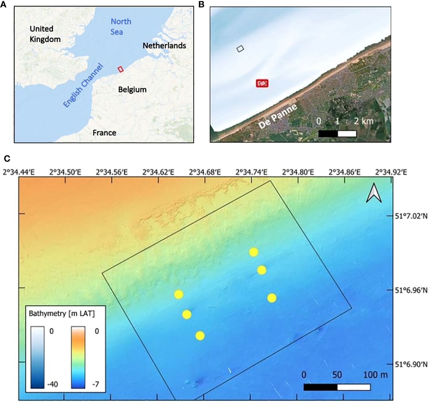
Figure 1. Location of aquaculture setup deployment sites off the coast of Belgium in the North Sea (A), near the city of De Panne (B). The longlines were deployed at an exposed site (black rectangle) and a sheltered site (red rectangle). Each side is composed of three long-lines (C) with 36 dropper lines, as represented in Figure 2. Base map: ESRI Ocean.

The longlines were spaced between 30 and 40 m apart at the sheltered site (Figure 1C) and between 20 and 50 m at the exposed site. Each longline was approximately 150 m long and consisted of a (near)surface line secured on the seabed by an anchor on either extremity. Two types of anchors were used at each site: a screw anchor, which was drilled directly into the seabed, and a block anchor with a chain attached to the end of the longline (Figure 2). Along the longlines, there were 36 three-meter-long mussel dropper lines, where mussel larvae could attach, spaced 1.5 m from each other. At the end of each dropper line, there was a concrete block weighing the lines down vertically in the water column. Buoys were attached to the longline in order to keep the longline occupied by dropper lines at the surface and not resting on the seabed. The mussel larvae were expected to settle on the dropper lines and metamorphose into the juvenile phase, allowing mussels to grow before dropping onto the seabed (Figure 2).

Figure 2

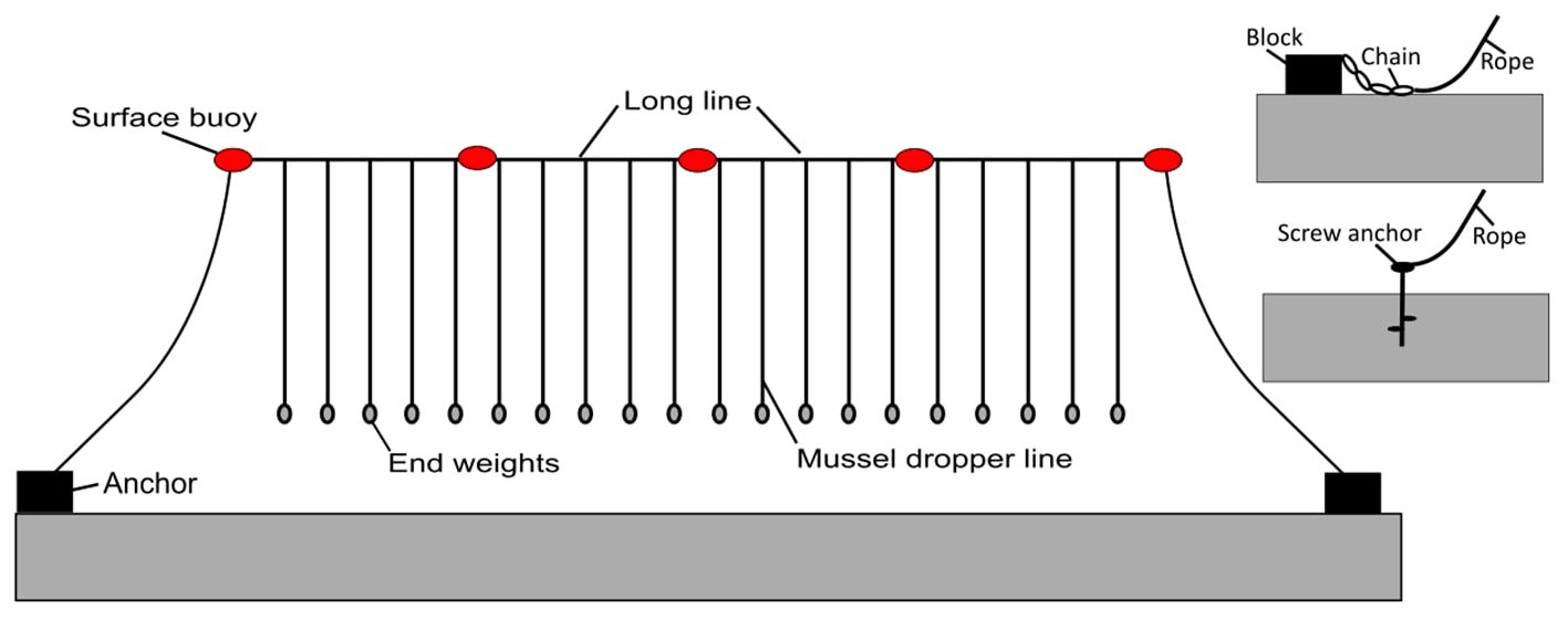
Figure 2. Sketch of the deployed structures in the context of the Coastbusters 2.0 project displaying longlines, surface buoys, dropper lines, end-weights, and anchors. Note that the sketch is not to scale; not all 36 dropper lines are represented in the figure. Three of these structures were deployed at each site.

The seabed in the region is mainly composed of sand with fine to medium grain size (Degraer et al., 2000), with an area of muddy sand to the south of the sheltered site. At both sites, the mussel longlines were deployed at a depth of 5 m LAT (lowest astronomical tide). The tide in the area is semi-diurnal with a range of 3.5 m during the neap tides and more than 5 m during spring tides. The large tidal range is associated with strong tidal currents, with peaks exceeding 1 m s^-1 in the nearshore area (Haerens et al., 2012).

Wind speed data from the Westinder weather and wave height data from the Trapegeer wave buoy (both from the Agency for Maritime Services and Coast, Flemish Government, 2023) were collected for the two survey years and months (Figure 3). The average prevailing wind and wave direction is southwesterly. However, because of the angle of the coast, the highest waves are generated when the wind is northwesterly (Fettweis et al., 2012). The winds were similar between the two months with the majority of the wind coming from the southwest. However, October has stronger winds in all directions and has periods of stronger winds and higher waves (Figures 3C–F). More northwesterly winds occur during October (Figures 3C, E) while August has periods of easterly winds (Figure 3A).

Figure 3

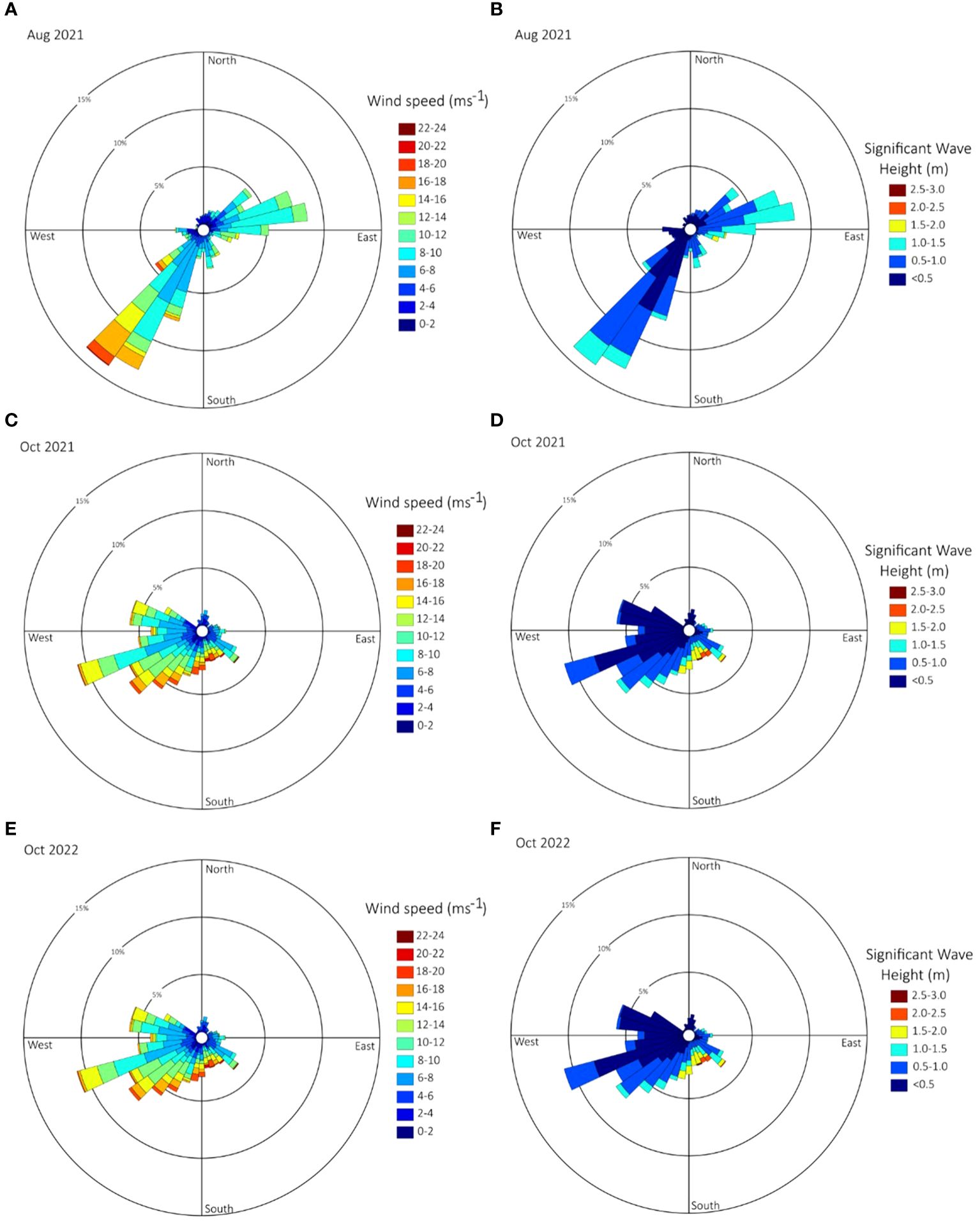
Figure 3. Wind speed and direction (A, C, E) from the Westinder weather station and significant wave height and direction (B, D, F) from the Trapegeer buoy for the year of 2021. Data was acquired from the Agency for Maritime Services and Coast, Flemish Government (2023).

2.2 AUV surveys

The AUV used in this research (AUV Barabas) is a commercial-off-the-shelf Teledyne Gavia modular vehicle (Figure 4A). For the surveys, it had a configuration of 2.87 m long, with a nose cone, a single battery pack module, and modules for navigation, control, surveying and propulsion. The AUV Barabas was equipped with an iXBlue Compact C5 inertial navigation system (INS) aided by a Pathfinder Doppler Velocity Log (DVL), European Geostationary Navigation Overlay Service-capable (EGNOS) Differential Global Positioning System (DGPS), and Keller pressure sensor (± 0.005 accuracy) (Figure 4A). The INS houses three fiber-optic gyros and three accelerometers. The data from the INS and the available aiding sensors are fed into a Kalman filter, which calculates a best guess of the position, speed, and altitude of the vehicle in all three dimensions, as well as their respective error estimates (Table 1). After starting the vehicle and prior to deployment, a continuous DGPS input is needed to align the INS. When the AUV Barabas is submerged, the combination of the Compact C5 INS and the Pathfinder DVL limits the increase in the position error to 0.02% of the distance travelled (CEP 50). Each time the AUV Barabas surfaces, the DGPS antenna will be able to obtain a new position fix, and the positioning error will decrease.

Figure 4

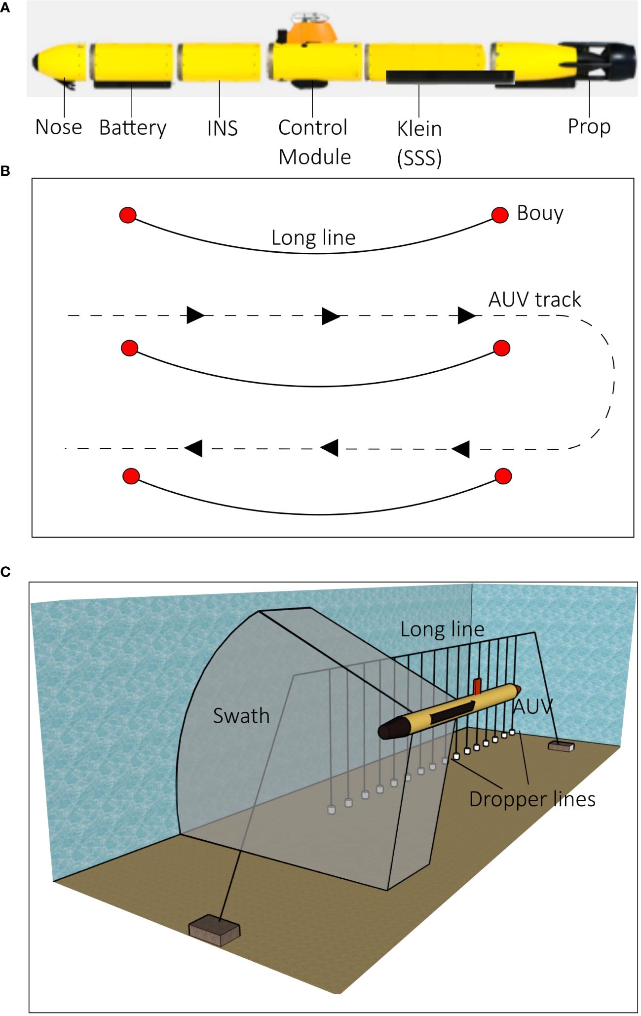
Figure 4. (A) Modules of the AUV Barabas used for the surveys, including the nose, battery, internal navigation system (INS), control module, Klein side scan sonar (SSS) module, and the prop. Typical survey pattern conducted by the AUV (B) and how it would fly next to the mussel longlines so that the side scan sonar could capture it (C). The image is a stylized representation and not to scale.

Table 1

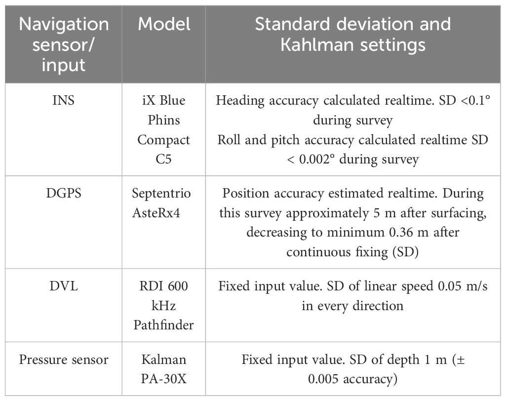
Table 1. Details and accuracy of AUV Barbara navigation equipment.

The speed of the AUV is vital to collect high quality side scan imagery, particularly in an environment with a strong current. The AUV’s speed can be set either as a fixed revolutions per minute (RPM) for the propeller or a fixed speed over ground (SOG). With a set RPM, the AUV’s SOG fluctuates with current speed, impacting data consistency. Alternatively, setting a fixed SOG allows real-time adjustment of propeller RPM for more consistent data, but affects maneuverability. Low RPM in current reduces maneuverability, while high RPM risks aggressive behavior and mission aborts. A minimum RPM of 500 and maximum of 1000 maintained stability, with an optimal SOG of 1.7 m s^-1 in background currents up to 0.5 m s^-1. For background currents with speed between 0.5 and 0.8 m s^-1, the AUV started to respond more erratically to disturbing factors. For background flow between 0.8 and 1 m s^-1, the AUV was still able to track a sampling line, but occasionally aborted the mission in the turn between lines, since it was unable to generate enough speed for drastic maneuvers. Above 1 m s^-1 currents, the increased risk of a mission abort and the reduced data made us decide not to deploy the AUV. Based on this empirical approach, the AUV Barabas sailed at a fixed speed over ground of 1.7 m s^-1 for this study, ensuring optimal flying mode and fixed sampling resolution to facilitate post-processing of the side scan sonar mosaic (see Section 2.3). At the very rear of the AUV, a nozzle contains the single propeller and four individually controlled fins. The fins thus control roll (actively maintaining 0° roll), pitch (used for depth control) and heading (used for track keeping). The AUV is not equipped with actuators to move laterally.

The AUV Barabas was successfully deployed in three campaigns (August and October 2021 and October 2022) equipped with a Klein 3500 dual-frequency interferometric side scan sonar (see details in Section 2.3) by the research vessel Simon Stevin. Several surveys of varying lengths were conducted for each campaign. Since the AUV Barabas was operating in-between and around the mussel longlines in a high-energy environment, a few considerations needed to be taken for each survey. The surveys were conducted with the AUV Barabas flying aligned either against or with the prevailing tidal current to prevent sideways movements of the vehicle, since this would lead to poor side scan sonar imagery. As mentioned above, navigation with AUVs is known to be challenging as vehicles lose GPS signals when underwater, and the error of INS increases the longer a vehicle is underwater (Wynn et al., 2014; Paull et al., 2018). To avoid collision with the longlines, the survey lines that passed closest to the obstacles were executed first when the position uncertainty was minimal. The mussel lines were installed parallel to the main current flow, but as the current turns with the tides, the mussel lines would curve between the anchors (either towards or away from the coast). This behavior was anticipated and taken into account when planning the survey tracks (Figure 4B). The track plan was relatively close to the longlines to ensure that they were captured in the side scan sonar swath (Figure 4C). However, the distance between the AUV Barabas and the longline would vary with the state of the tide and the ambient current.

2.3 Data collection, processing, and analyses

Side scan sonar operates by emitting a signal, commonly referred to as a “beam”, which travels through the water column and reaches the seafloor or structures located on either side of the sampling platform. This platform is typically a towfish or vessel (Blondel, 2009). In our study, however, the side scan sonar was mounted on an AUV (e.g., Wynn et al., 2014). The AUV Barabas was equipped with a Klein 3500 dual-frequency interferometric side scan sonar. Figure 4A shows the positioning of the side scan sonar system on the vehicle. Once the data was collected, it was displayed and processed using two different methods: waterfall and mosaics. The raw data was plotted as waterfall images using the SonarPro software (version 14.1, Klein Marine Systems, Inc). Waterfall images depict the intensity of the sonar signal return. While various methods exist for presenting waterfall images, in this study, distances are plotted along the x-axis, with increasing distance from the center of the figure. Additionally, successive data samples are represented along the y-axis, which corresponds to both time and distance, considering the sampling rate and the vehicle’s cruising speed. Waterfall images enable the identification and measurement of features and contacts, as well as the acquisition of individual positions. However, due to the extensive number of samples, only a fraction of the data can be displayed. Additionally, these images cannot be integrated with other data sources due to the absence of georeferencing.

On the other hand, the mosaics are georeferenced images and were created with SonarWiz software (SonarWiz 7, Chesapeake Technology, Inc), where movements of the AUV Barabas (pitch, roll, and yaw) are also compensated for. Depending on the quality and quantity of the images, building a mosaic can be labor intensive, requiring specialized software and some resolution can be lost. A mosaic can be exported in a wide range of data formats, allowing the data to be overlaid with other georeferenced data.

As a dual-frequency system, the sonar transducer emitted acoustic signals at two distinct frequencies: a relatively high frequency of 900 kHz and a relatively low frequency of 455 kHz. The high-frequency (900 kHz) beam has a horizontal opening angle of 0.34°, and the range (single side) can be set between 15 m and 75 m. The low-frequency (455 kHz) beam had a horizontal opening angle of 0.48°, and the range could be set between 30 m and 200 m. The optimal altitude above the seafloor is 10–15% of the sonar range, meaning that the operational range of the sonar will be limited by the local depth. The along-track sampling is inversely proportional to the AUV’s sailing speed and sonar range, whereas the cross-track resolution of the side scan sonar’s Compressed High Intensity Radar Pulse (CHIRP) relies on the sampling frequency. A variety of side scan sonar settings were tested during each survey to define which settings obtained the most useful data. The altitudes tested were 3 m and 5 m, with corresponding ranges of 30 m and 50 m. Both high-frequency and low-frequency data were collected simultaneously. Finally, pulse lengths of 2 ms and 1 ms were tested, with a respective sampling frequency of 31250 Hz and 62500 Hz, providing an across track resolution of 4.8 cm and 2.4 cm.

3 Results and discussion

3.1 Optimizing AUV surveys and side scan sonar settings

For this research, high and low-frequency transducer settings were used and analyzed both in a waterfall display and as mosaic images. The high frequency was used for the analysis as it provides the highest resolution of the data. The low-frequency setting was run at the same time and was used for redundancy.

The survey area is affected by wind and wave action, which impact the AUV Barabas and the quality of side scan sonar data when the vehicle is close to the sea surface. Therefore, the altitude of the AUV Barabas combined with the tidal height is critical. There were two main survey heights: 3 and 5 m from the seabed. At 5 m, roll artefacts were seen in both the waterfall and in the mosaic data (Figure 5A). The mosaic looked ‘wavy’ and had shading in places where there is no object to cast an acoustic shadow (Figure 5A). It is clear that the AUV Barabas was too close to the surface and was being excessively impacted by the surface waves. When the survey height was set at 3 m from the seabed, the roll artefacts were significantly reduced (Figure 5B). With the survey site being relatively shallow, even small surface waves (<0.5 m) will have more of an effect on the AUV Barabas, reducing the operational window in which the largest coverage and highest quality of data can be obtained. The altitude of the AUV Barabas affects the maximum distance that can be imaged by the side scan sonar, which is also known as the range. In general, a lower range provides a higher image resolution but covers a smaller area of the seabed. A range of 10 times the altitude was found to cover the largest area while providing the highest resolution (Flemming, 1976). In the three campaigns, two ranges were used: 30 m and 50 m. Since 3 m altitude produced better quality data, it became the predominant survey altitude and, therefore, 30 m became the predominant acoustic range used.

Figure 5

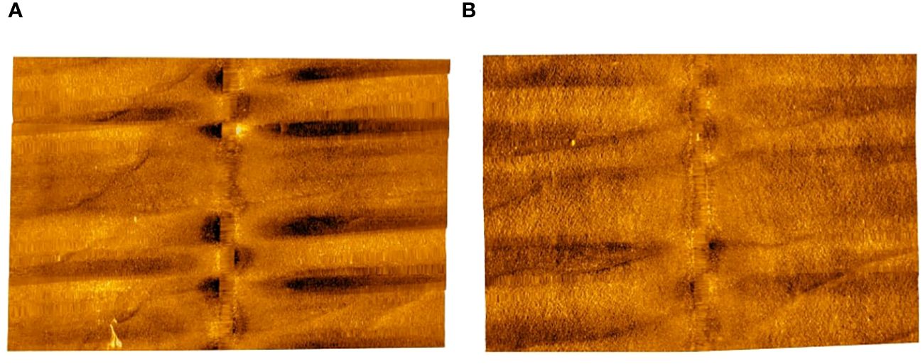
Figure 5. Images showing the difference in the quality of side scan sonar data at a relatively high altitude of 5 m (A) and low altitude of 3 m from the seabed (B). The side scan sonar data settings were as follows: frequency 950 kHz, altitude 5 m (A) and 3 m (B), range 50 m (A) and 30 m (B), pulse length 2 ms. Both images have had the same degree of processing applied.

Throughout the campaigns, different surveys used a pulse length of either 2 ms (31250 Hz sampling frequency) or 1 ms (62500 Hz sampling frequency), as shown in Figure 6. We found the higher across track resolution of the 1 ms pulse length to provide a clearer image when analyzing the objects on the seabed in the waterfall, such as an anchor (Figure 6A, B). However, when using the mosaic format, we found that the higher resolution provided little added value, and the contrast between the seabed and objects on the seabed decreased (Figure 6C). Therefore, a pulse length of 2 ms is better suited for mosaics, as it creates a clearer image of the seabed and provides better contrast between objects (Figure 6D). This could be clarified by the stretching of pixels when georeferencing: at a sonar range of 30 m and sailing at 1.7 m s^-1, the along-track sampling resolution is 6.8 cm, which is closer to the across-track resolution of the 2 ms pulse (4.8 cm) than to that of the 1 ms pulse (2.4 cm). When using side scan sonar mosaics and waterfall together, the choice of pulse length depends on the specific mission objectives.

Figure 6

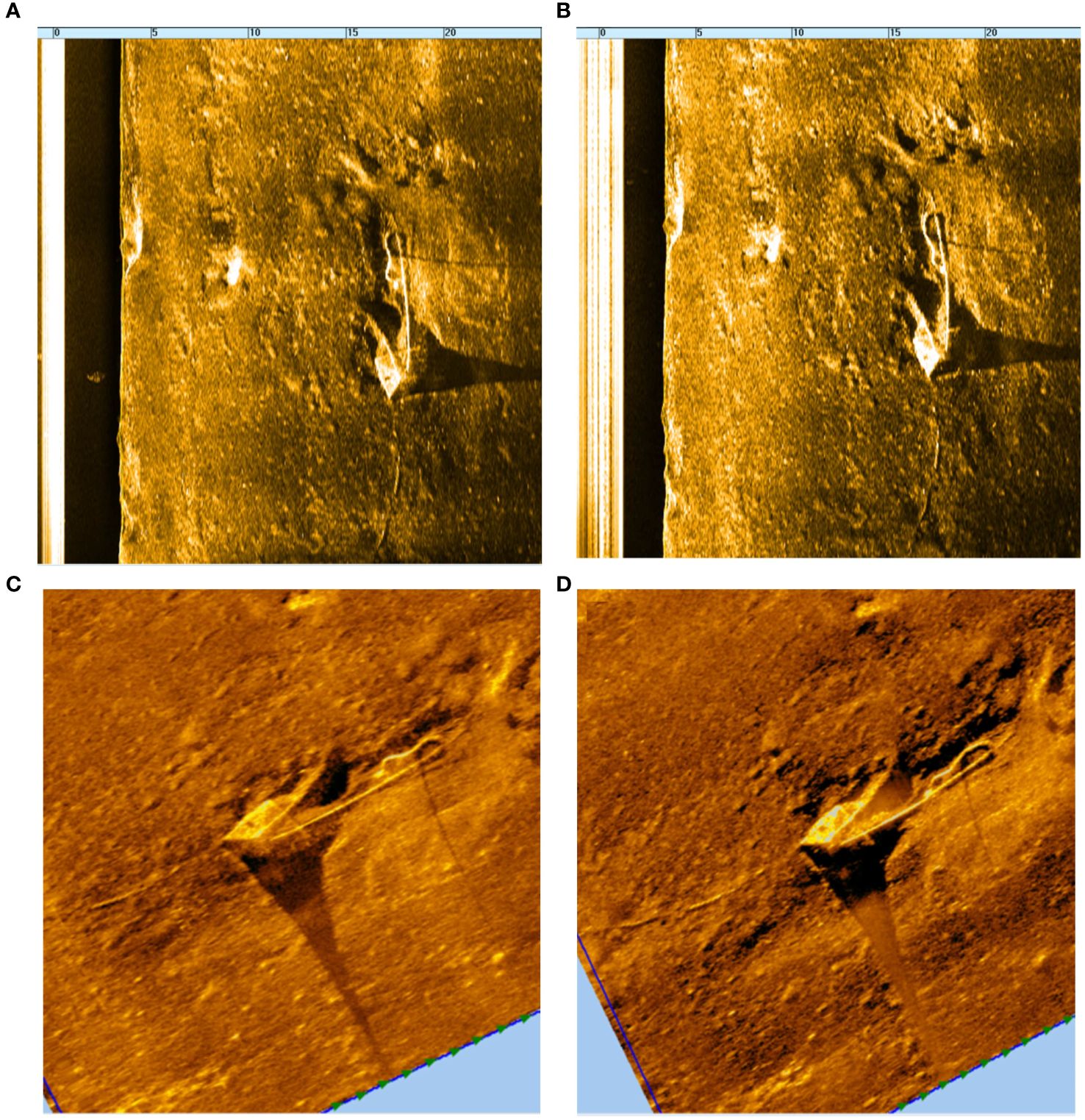
Figure 6. Waterfall and mosaic images of an anchor on the seafloor comparing the two pulse rates used 1 ms (A, C) and 2 ms (B, D). The other side scan sonar data settings were as followed: Frequency 950 kHz, Altitude 5 m, Range 30m.

3.2 Aquaculture setup inspection

The most data was collected from the sheltered site and is only data analyzed in the following section. The images captured by the side scan sonar on the AUV Barabas clearly show the mussel longlines in both the waterfall and the mosaics, even when the longlines are above the transducer and sometimes at the surface of the water column. When compiling the survey images together into a mosaic, it is possible to see all three longlines (Figures 7, 8). Using this technique, a surveyor can confirm that the lines and their anchors are still intact and assess how the lines are being impacted by the local currents. An example of this is the distinctive curve of the longlines as they are pushed in the direction of the tide, curving towards the shore during the flood current or away from the shore during the ebb current (Figures 7, 8).

Figure 7

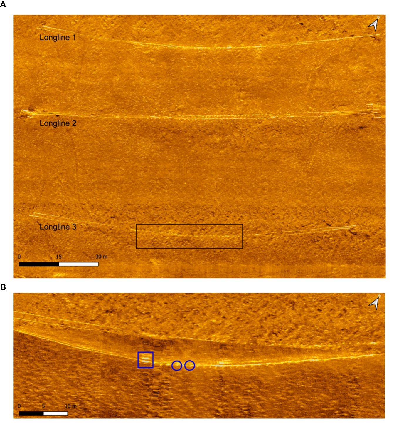
Figure 7. Side scan sonar mosaic of the sheltered site conducted in August 2021, with the three mussel longlines clearly visible (A) and the individual mussel dropper lines (B). Some of the individual dropper lines are highlighted in blue, with the square indicating a surface buoy on the longline. The side scan sonar data settings were as follows: frequency 950 kHz, altitude 3 m, range 30 m, pulse length 2 ms.

Figure 8

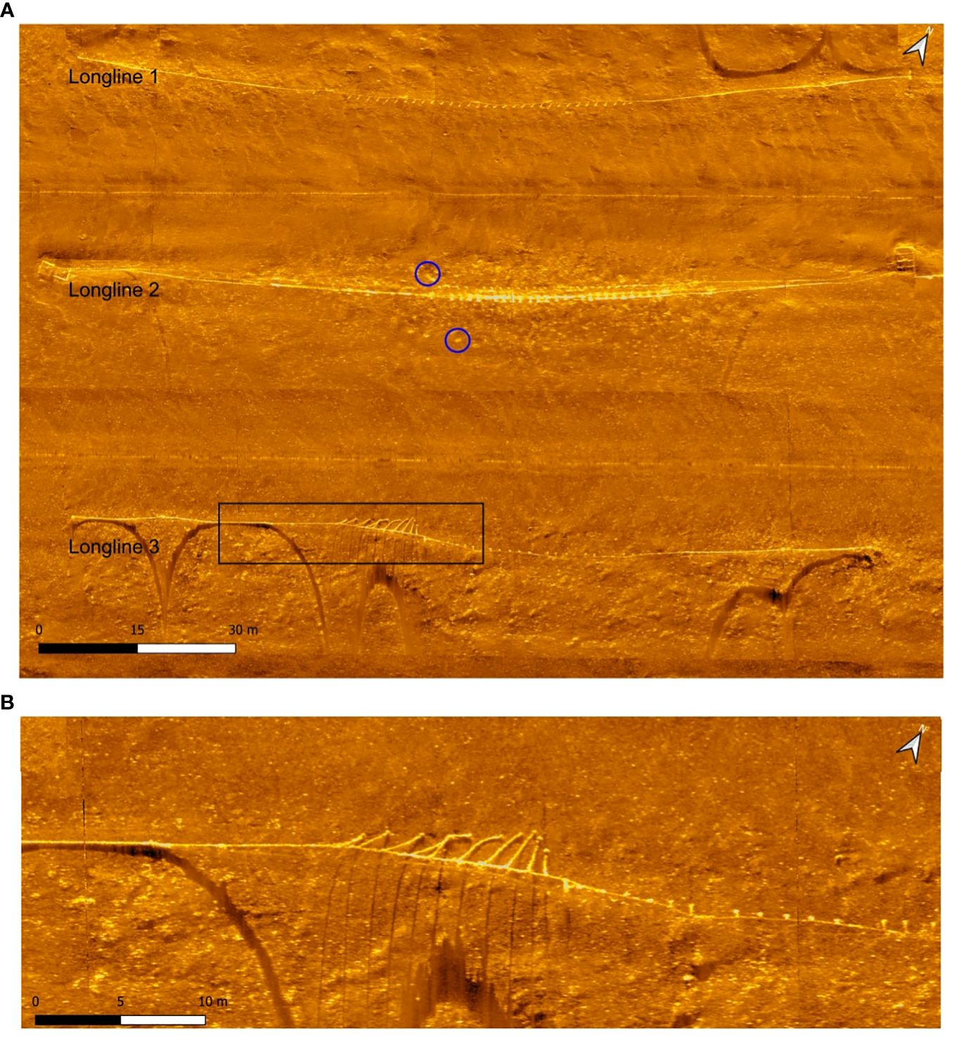
Figure 8. Side scan sonar mosaic of the sheltered site conducted in October 2021, with the three mussel longlines clearly visible. Potential contacts of mussels on the seafloor are highlighted in blue (A). Individual mussel dropper lines resting on the seabed (B). The side scan sonar data settings were as follows: frequency 950 kHz, altitude 3 m, range 30 m, pulse length 2 ms.

In addition to the mosaics, the waterfall images show the individual dropper lines as the AUV Barabas flies parallel to the lines, and if the dropper lines are not visible, the acoustic shadows often appear (Figure 9). The shadows not only show that the mussel dropper lines are intact, but by using SonarPro and measuring the distance between the start of the shadow and the dropper line, one can determine their height above the seabed (Figure 9). From analyzing the waterfall image (Figure 9), there are three places where the shadow of the longline or the dropper lines touch the respective reflections, indicating that the objects are on the seabed. Looking in further detail at the mussel dropper lines at the top of the image, there are nine on the seabed. The dropper lines then quickly rise off the seabed with an increase of 1.2 m between dropper lines 2 and 3 (Figure 9).

Figure 9

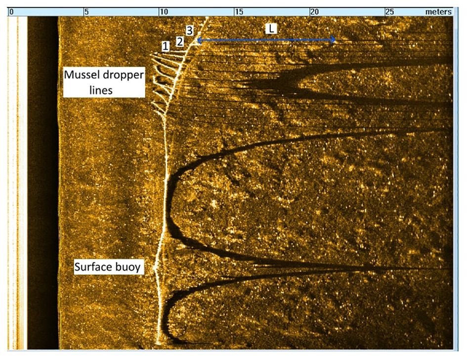
Figure 9. Waterfall images displaying of the longline and mussel dropper lines. L is the measured distance between the acoustic shadow and the object, used to calculate the height of bottom of surface buoy = 2.1 m, dropper line 1 = 0 m, dropper line 2 = 0.36m and dropper line 3 = 1.5m. The side scan sonar data settings were as follows: frequency 950 kHz, altitude 3 m, range 30 m, pulse length 2 ms.

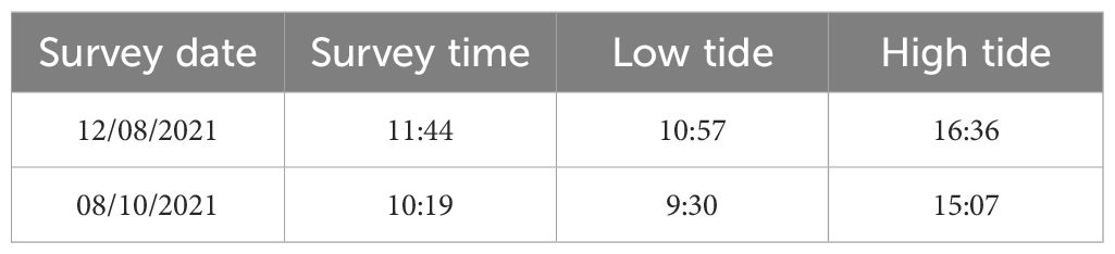
Using the AUV Barabas to conduct repeated surveys provides insight into how the longlines might change over time. The August 2021 survey (Figure 7B) was able to pick out the buoys on the line and the dropper lines. When the entire dropper line is at approximately the same distance from the transducer, the dropper lines are displayed as dots, highlighted in blue, similar to a top-side view. The same survey was conducted in October 2021 (Figure 8B), and in this survey, some dropper lines were visibly resting on the seabed. The two surveys were conducted at similar states of tide (Table 2), so this could indicate that the mussel dropper lines were heavier in October than in August, suggesting there had been mussel growth compatible with the relatively higher mussel growth and ventral thickness of the shells expected at this time of the year (Nagarajan et al., 2006). The dropper lines on longline 3 were clearly dragged along the seabed, as this longline does not have a uniform curve like lines 1 and 2 (Figure 8A). With the mussel dropper lines resting on the seabed, they are at risk of entanglement (Figure 8B). They add extra stress on the longline and will also impact the surrounding seabed as the dropper lines are dragged back and forth with the tide. From an aquaculture perspective, the dropper lines should avoid touching the seabed, as the quality of the mussels will be impacted. It is well known that mussels suspended in the water column produce a higher yield, as they are able to feed constantly and require less cleaning to remove sand and grit before consumption (Cheong and Lee, 1984). From a reef building perspective (as is the case for the Coastbusters 2.0 project), dropper lines on the seafloor could hamper the creation of a reef. As the dropper lines are dragged along the seabed with tidal currents, the concrete weights at the end of the line can induce significant scour and disturb any organisms on the seabed.

Table 2

Table 2. Tidal information during AUV Barabas surveys displayed in Figures 5 and 6.

3.3 Seabed inspection and environmental impact

Using side scan sonar to detect objects, such as reefs or shipwrecks, and monitor scouring on the seabed is a common practice (Johnson and Helferty, 1990; Penrose et al., 2005). Our surveys indicated both mussels on the seabed and seabed scouring from the aquaculture setup. The surveys conducted in October 2021 detected a large number of reflections that appeared as bright spots surrounding longline 2 (Figure 8A). The reflections are similar to how mussels appear on side scan sonar in previous studies (Powers et al., 2015) and mussels were found beneath long lines by diving surveys in summer and winter of 2021, but no surveys were conducted when the data for Figure 8A was collected (Islam et al., 2024).

The AUV itself will have very little impact on the environment and the seafloor as it needs to be kept at least 3 m off the seabed in order to collect high quality side scan data as discussed in section 2.2. The Gavia AUV is also battery powered and contributes to the decarbonization of marine fleets. However, the mussel long lines can negatively impact the seabed. Although longlines are deployed in high-energy environments where the sediment is routinely disturbed, scouring can still have an impact on benthic habitats (Broad et al., 2020) and can potentially release carbon stored in the seafloor, which may then enter the atmosphere (Atwood et al., 2024). From analyzing the side scan imagery, the scouring is most significant around the block anchors for the mussel longlines (Figure 10). Scouring is important to monitor, especially in shallow high-energy environments, as it is well known to affect the stability of structures on the seabed (Sumer and Fredsøe, 2002). For the two types of anchors (screw and block anchors, as described in Section 2.1), there are different degrees of scouring. The screw anchor shows no evidence of scouring, while there is significant scouring around the block and chain anchor (Figure 10). There is a large pit around the block and under the chain, which is a result of the tidal current pushing the chain back and forth. Scouring was more apparent in waterfall images than in mosaics, where the processing and combining of survey tracks reduced the appearance of anchor pits. Anchors and their chains are well known to create pits and displace sediments. These sediments usually support a variety of marine life, including polychaetes, crustaceans, mollusks, and sponges, all of which are vulnerable to anchors and their associated scour (Sorokin et al., 2005; Pitcher et al., 2009). Given that there is no scouring present when using a screw anchor, it would be the preferable method of the two anchors used here for mussel longline deployment to prevent the unintentional destruction of a potential mussel reef.

Figure 10

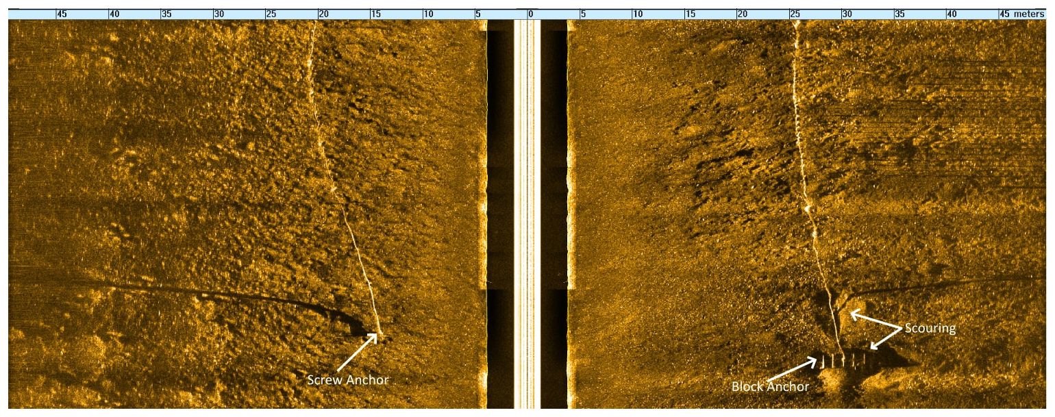
Figure 10. Waterfall images of significant scouring around the two different anchors of the mussel longlines, a screw anchor (left) and block anchor (right). The side scan sonar data settings were as follows: frequency 950 kHz, altitude 5 m, range 50 m, pulse length 2 m.

4 Summary and conclusions

The objective of this study was to test the following hypothesis: “AUVs equipped with interferometric side scan sonar can effectively monitor mussel aquaculture installations, including long- and dropper lines, anchoring systems, and the seabed beneath, in high-energy and turbid environments”. To address this hypothesis the following four questions were raised. First, can an AUV safely conduct surveys of aquaculture infrastructure in shallow and turbid, high-energy environments? Three campaigns and several surveys were successfully conducted in and around the mussel lines in the Belgian North Sea, an area with current speed exceeding 1 m s^-1. This study shows that side scan sonar mounted on an AUV is a viable technique in support of management of aquaculture and coastal protection setups. Apart from mapping the seabed, structures in the water column can be detected and analyzed. Using an AUV in a shallow, high-energy environment is not without challenges. The strong current and waves associated with the high-energy environment can cause roll, which has the greatest impact on the quality of the side scan sonar data (Figure 4). To combat the strong currents, AUV Barabas was aligned either against or with the prevailing tidal current to prevent the instrument from moving sideways. The speed of the AUV was also set a fixed SOG of 1.7 m s^-1 as that was found to be the best for the current conditions and provided the best quality of data. The impact of surface waves was addressed by flying the AUV Barabas at a lower altitude; however, the AUV Barabas still needed to be high enough to detect the mussel longlines on the surface. The close proximity to submerged obstacles called for a high navigational accuracy, which was ensured by planning short missions with intermittent GPS fixes.

The second question was: which side scan sonar settings yield the highest quality data? The altitude of the AUV impacts coverage of the side scan sonar. With the AUV Barabas at a lower altitude (3 m instead of 5 m from the seabed) to avoid impact from surface waves, the range is lower and covers less of the seabed. However, the resolution is higher and the AUV will pitch and roll less, providing more detailed images. As expected the high frequency setting (900 kHz) produced the highest data resolution. The quality of the data produced by the two pulse lengths used depended upon the format in which the data was displayed. In the mosaic, a pulse length of 2 ms provided better data, whereas a pulse length of 1 ms provided more detail when displayed in the waterfall.

The third question was: what relevant information could be ascertained about the aquaculture setup? The surveys provided details on not only the longlines and their anchors but also the individual dropper lines in the water column. The surveys show how far the dropper lines are above the seabed and when they rest upon it. This is relevant for both aquaculture setups, as it provides insight into the stressors placed on longlines in high-energy environments and the impact of the setup on the seabed. If the survey shows the dropper lines on the seabed, the entire setup can be properly adjusted to ensure that the mussel dropper lines stay above the seabed. This is critical for both the quality of the mussels harvested in aquaculture and the development of a mussel reef for coastal protection.

Finally, we addressed the fourth question to investigate what pertinent information can be unraveled about the seabed surrounding the aquaculture setup and, therefore, investigated the potential impact on the seabed. The side scan sonar surveys also collected data on the surrounding environment and show that the main impact of the aquaculture setup on the seabed is scouring, particularly around the anchors. A traditional block and chain anchor induces significantly more scouring than a screw anchor. Scouring from the anchor could affect not only organisms in the surface substrate but also any mussels that settle on the seabed from the dropper lines.

The results demonstrate that employing an Autonomous Underwater Vehicle (AUV) equipped with a side scan sonar is a viable and innovative technique for monitoring mussel longlines. As these techniques continue to evolve, they could offer a more cost-effective and simpler alternative to the traditionally challenging logistics of conventional monitoring methods. This advancement underscores the potential for significant enhancements in aquaculture management, particularly in optimizing operational efficiencies and reducing risks. However, monitoring with an AUV is not without drawbacks. Side scan sonar does not provide direct information on the health of the mussels setup such as occurrence of predators or fouling. The positioning error from underwater navigation increases the longer the AUV is under the water. Therefore, shorter and more frequent dives with surfacing to regain accurate positioning from satellite navigation systems might be required.

Another limitation is the size of the AUV itself. With a length of almost 3 m, the used AUV Barabas has a relatively large turning radius, which is not ideal for a lawnmower pattern flown between two mussel longlines. The size and weight also require a support vessel for safe launch and recovery. Since most of our findings are not specific to the AUV Barabas used, the issues could be overcome by using smaller AUVs. Smaller, cheaper AUVs are emerging on the market, and while they are unable to match the sonar range, depth rating, and navigation precision of a survey class AUV, these factors might be less of a concern in very shallow water. The data quality could be sufficient for operational monitoring, with much lower acquisition costs and a minimal logistical footprint.

The approach used in this study shows that it is an efficient and safe alternative to combine AUVs and side scan sonar in the detailed monitoring of an aquaculture setup. A similar approach could be implemented in the monitoring of offshore mussel farms at a large production scale, allowing for intense monitoring in short periods. This monitoring strategy could also be suitable for other aquaculture setups. For example to monitor structural integrity of pisciculture cages, oyster cages/beds, and more particularly their impact on the seafloor. The AUV platform allows for multiple sensors to be collecting data at once so environmental data could be collected along with side scan sonar data, providing information on temperature, salinity and water pH. Using an AUV also provides a low risk alternative to site inspection to either identify suitable areas for aquaculture installations or after disaster, such as structural damage after a storm. Monitoring aquaculture setups with an AUV could also be used in tandem with other marine robotic platforms such an ROV. An AUV survey would provide information about a site as a whole, then an ROV could perform detailed visual inspection on areas of interest and look at specific problems for example biofouling on the mussels.

Data availability statement

The raw data supporting the conclusions of this article will be made available by the authors, without undue reservation.

Author contributions

CP: Formal analysis, Visualization, Writing – original draft, Writing – review & editing. KL: Conceptualization, Data curation, Formal Analysis, Investigation, Methodology, Writing – original draft, Writing – review & editing. FF: Data curation, Methodology, Writing – review & editing, Conceptualization, Investigation. LP: Writing – original draft, Writing – review & editing. IM: Writing – review & editing. AS: Writing – review & editing. TS: Writing – review & editing. RG: Writing – review & editing. BG: Writing – review & editing. WB: Conceptualization, Funding acquisition, Project administration, Resources, Supervision, Writing – original draft, Writing – review & editing.

Funding

The author(s) declare financial support was received for the research, authorship, and/or publication of this article. This research was part of the Blue Cluster Project Coastbusters 2.0 and funded by Flanders Innovation & Entrepreneurship (VLAIO) through the funding HBC.2019.0037. Blue Cluster was not involved in the study design, collection, analysis, interpretation of data, the writing of this article, or the decision to submit it for publication.

Acknowledgments

We would like to acknowledge Flanders Innovation & Entrepreneurship (VLAIO) and Blue Cluster for funding the Coastbusters 2.0 Project. Furthermore, we gratefully acknowledge the crew of RV Simon Stevin and DAB Vloot for their continuous support in performing the research at sea. Finally, we thank the Marine Robotics Center (MRC) of the Flanders Marine Institute (VLIZ) for the use of AUV Barabas in our research.

Conflict of interest

Author TS was employed by company DEME Group. Author RG was employed by company Jan De Nul. Author BG was employed by company Sioen Industries NV.

The remaining authors declare that the research was conducted in the absence of any commercial or financial relationships that could be construed as a potential conflict of interest.

Publisher’s note

All claims expressed in this article are solely those of the authors and do not necessarily represent those of their affiliated organizations, or those of the publisher, the editors and the reviewers. Any product that may be evaluated in this article, or claim that may be made by its manufacturer, is not guaranteed or endorsed by the publisher.

References

Agency for Maritime Services and Coast, Flemish Government. (2023). Flemish banks monitoring network. Available at: https://meetnetvlaamsebanken.be/.

Google Scholar

Ali A., Abdullah M. R., Safuan C. D. M., Afiq-Firdaus A. M., Bachok Z., Akhir M. F. M., et al. (2022). Side-scan sonar coupled with scuba diving observation for enhanced monitoring of benthic artificial reefs along the coast of Terengganu, Peninsular Malaysia. J. Mar. Sci. Eng. 10, 1309. doi: 10.3390/jmse10091309

Crossref Full Text | Google Scholar

Allison E. H. (2011). Aquaculture, fisheries, poverty and food security (Penang: The WorldFish Center), 62. Working Paper 2011-65.

Google Scholar

Amundsen H. B., Caharija W., Pettersen K. Y. (2021). Autonomous ROV inspections of aquaculture net pens using DVL. IEEE J. Oceanic Eng. 47, 1–19. doi: 10.1109/JOE.2021.3105285

Crossref Full Text | Google Scholar

Atwood T. B., Romanou A., DeVries T., Lerner P. E., Mayorga J. S., Bradley D., et al. (2024). Atmospheric CO2 emissions and ocean acidification from bottom-trawling. Front. Mar. Sci. 10, 1125137. doi: 10.3389/fmars.2023.1125137

Crossref Full Text | Google Scholar

Avdelas L., Avdic‐Mravlje E., Borges Marques A. C., Cano S., Capelle J. J., Carvalho N., et al. (2021). The decline of mussel aquaculture in the European Union: causes, economic impacts and opportunities. Rev. Aquaculture 13, 91–118. doi: 10.1111/raq.12465

Crossref Full Text | Google Scholar

Bao J., Li D., Qiao X., Rauschenbach T. (2020). Integrated navigation for autonomous underwater vehicles in aquaculture: A review. Inf. Process. Agric. 7, pp.139–pp.151. doi: 10.1016/j.inpa.2019.04.003

Crossref Full Text | Google Scholar

Barbosa R. V., Jaud M., Bacher C., Kerjean Y., Jean F., Ammann J., et al. (2022). High-resolution drone images show that the distribution of mussels depends on microhabitat features of intertidal rocky shores. Remote Sens. 14, 5441. doi: 10.3390/rs14215441

Crossref Full Text | Google Scholar

Blondel P. (2009). “The Handbook of Sidescan Sonar.” in Springer Praxis Books (Berlin, Heidelberg: Springer). doi: 10.1007/978-3-540-49886-5_4

Crossref Full Text | Google Scholar

Borsje B. W., van Wesenbeeck B. K., Dekker F., Paalvast P., Bouma T. J., van Katwijk M. M., et al. (2011). How ecological engineering can serve in coastal protection. Ecol. Eng. 37, 113–122. doi: 10.1016/j.ecoleng.2010.11.027

Crossref Full Text | Google Scholar

Boulenger A., Lanza-Arroyo P., Langedock K., Semeraro A., Van Hoey G. (2024). Nature-based solutions for coastal protection in sheltered and exposed coastal waters: integrated monitoring program for baseline ecological structure and functioning assessment. Environ. Monit. Assess. 196, 316. doi: 10.1007/s10661-024-12480-x

PubMed Abstract | Crossref Full Text | Google Scholar

Brehmer P., Gerlotto F., Guillard J., Sanguinède F., Guénnegan Y., Buestel D. (2003). New applications of hydroacoustic methods for monitoring shallow water aquatic ecosystems: the case of mussel culture grounds. Aquat. Living Resour. 16, 333–338. doi: 10.1016/S0990-7440(03)00042-1

Crossref Full Text | Google Scholar

Brehmer P., Vercelli C., Gerlotto F., Sanguinède F., Pichot Y., Guennégan Y., et al. (2006). Multibeam sonar detection of suspended mussel culture grounds in the open sea: Direct observation methods for management purposes. Aquaculture 252, 234–241. doi: 10.1016/j.aquaculture.2005.06.035

Crossref Full Text | Google Scholar

Broad A., Rees M. J., Davis A. R. (2020). Anchor and chain scour as disturbance agents in benthic environments: trends in the literature and charting a course to more sustainable boating and shipping. Mar. pollut. Bull. 161, 111683. doi: 10.1016/j.marpolbul.2020.111683

PubMed Abstract | Crossref Full Text | Google Scholar

Bryant R. S. (1975). “Side Scan Sonar for Hydrography - An Evaluation by the Canadian Hydrographic Service”, The International Hydrographic Review. 52 (1).

Google Scholar

Cheong L., Lee H. B. (1984). Mussel farming (Bangkok, Thailand: Secretariat, Southeast Asian Fisheries Development Center).

Google Scholar

Clausner J. E., Pope J. (1988). May. “Application of side-scan sonar for inspection of coastal structures.” in Offshore Technology Conference. (OTC), OTC–5781. doi: 10.4043/5781-MS

Crossref Full Text | Google Scholar

Degraer S., Van Lancker V., Moerkerke G., Van Hoey G., Vincx M., Jacobs P., et al. (2000). Intensive evaluation of the evolution of a protected benthic habitat. HABITAT RUG Section Mar. Biology-Sedimentary geology Eng. geology, 1–16.

Google Scholar

Ells K., Murray A. B. (2012). Long-term, non-local coastline responses to local shoreline stabilization. Geophysical Res. Lett. 39. doi: 10.1029/2012GL052627

Crossref Full Text | Google Scholar

Fettweis M., Baeye M., Lee B. J., Chen P., Yu J. C. (2012). Hydro-meteorological influences and multimodal suspended particle size distributions in the Belgian nearshore area (southern North Sea). Geo-Marine Lett. 32, 123–137. doi: 10.1007/SÛ0367-011-0266-7

Crossref Full Text | Google Scholar

Flemming B. W. (1976). Side-scan sonar: a practical guide. Int. hydrographic Rev. 53, 65–92.

Google Scholar

Goedefroo N., Benham P., Debusschere E., Deneudt K., Mascart T., Semeraro A., et al. (2022). Nature-based solutions in a sandy foreshore: A biological assessment of a longline mussel aquaculture technique to establish subtidal reefs. Ecol. Eng. 185, 106807. doi: 10.1016/j.ecoleng.2022.106807

Crossref Full Text | Google Scholar

Greene A., Rahman A. F., Kline R., Rahman M. S. (2018). Side scan sonar: A cost-efficient alternative method for measuring seagrass cover in shallow environments. Estuarine Coast. Shelf Sci. 207, 250–258. doi: 10.1016/j.ecss.2018.04.017

Crossref Full Text | Google Scholar

Greene H. G., Yoklavich M. M., Starr R. M., O’Connell V. M., Wakefield W. W., Sullivan D. E., et al. (1999). A classification scheme for deep seafloor habitats. Oceanol. Acta 22, 663–678. doi: 10.1016/S0399-1784(00)88957-4

Crossref Full Text | Google Scholar

Haerens P., Bolle A., Trouw K., Houthuys R. (2012). Definition of storm thresholds for significant morphological change of the sandy beaches along the Belgian coastline. Geomorphology 143, 104–117. doi: 10.1016/j.geomorph.2011.09.015

Crossref Full Text | Google Scholar

Hicks D., Cintra-Buenrostro C., Kline R., Shively D., Shipley-Lozano B. (2015). “Artificial reef fish survey methods: counts vs. Log-categories yield different diversity estimates,” in Proceedings of the 68th Gulf and Caribbean Fisheries Institute, 74–79. Available online at: https://www.REEF.org.

Google Scholar

Hou S., Jiao D., Dong B., Wang H., Wu G. (2022). Underwater inspection of bridge substructures using sonar and deep convolutional network. Advanced Eng. Inf. 52, 101545. doi: 10.1016/j.aei.2022.101545

Crossref Full Text | Google Scholar

Islam M., Semeraro A., Langedock K., Moulaert I., Stratigaki V., Sterckx T., et al. (2024). Inducing mussel beds, based on an aquaculture long-line system, as nature-based solutions: effects on seabed dynamics and benthic communities. Nature-Based Solutions 6, 100142. doi: 10.1016/j.nbsj.2024.100142

Crossref Full Text | Google Scholar

Johnson H. P., Helferty M. (1990). The geological interpretation of side scan sonar. Rev. Geophys. 28, 357. doi: 10.1029/RG028i004p00357

Crossref Full Text | Google Scholar

Karimanzira D., Jacobi M., Pfützenreuter T., Rauschenbach T., Eichhorn M., Taubert R., et al. (2014). First testing of an AUV mission planning and guidance system for water quality monitoring and fish behavior observation in net cage fish farming. Inf. Process. Agric. 1, 131–140. doi: 10.1016/j.inpa.2014.12.001

Crossref Full Text | Google Scholar

Koch E. W., Barbier E. B., Silliman B. R., Reed D. J., Perillo G. M., Hacker S. D., et al. (2009). Non-linearity in ecosystem services: temporal and spatial variability in coastal protection. Front. Ecol. Environ. 7, 29–37. doi: 10.1890/080126

Crossref Full Text | Google Scholar

Krull W., Berry P., Bauduceau N., Cecchi C., Elmqvist T., Fernandez M., et al. (2015). Towards an EU research and innovation policy agenda for nature-based solutions & re-naturing cities. Final report of the Horizon 2020 expert group on nature-based solutions and re-naturing cities., 1–70. doi: 10.2777/479582

Crossref Full Text | Google Scholar

Lowry M. B., Glasby T. M., Boys C. A., Folpp H., Suthers I., Gregson M. (2014). Response of fish communities to the deployment of estuarine artificial reefs for fisheries enhancement. Fisheries Manage. Ecol. 21, 42–56. doi: 10.1111/fme.12048

Crossref Full Text | Google Scholar

Marsden J. E., Marcy-Quay B., Dingledine N., Berndt A., Adams J. (2023). Physical and biological evolution of constructed reefs–long-term assessment and lessons learned. J. Great Lakes Res. 49, 276–287. doi: 10.1016/j.jglr.2022.10.008

Crossref Full Text | Google Scholar

Massarelli C., Galeone C., Savino I., Campanale C., Uricchio V. F. (2021). Towards sustainable management of mussel farming through high-resolution images and open source software—The taranto case study. Remote Sens. 13, 2985. doi: 10.3390/rs13152985

Crossref Full Text | Google Scholar

McGeady R., Runya R. M., Dooley J. S., Howe J. A., Fox C. J., Wheeler A. J., et al. (2023). A review of new and existing non-extractive techniques for monitoring marine protected areas. Front. Mar. Sci. 10, 1126301. doi: 10.3389/fmars.2023.1126301

Crossref Full Text | Google Scholar

Mitchell N. C., Somers M. L. (1989). Quantitative backscatter measurements with a long-range side-scan sonar. IEEE J. Oceanic Eng. 14, pp.368–pp.374. doi: 10.1109/48.35987

Crossref Full Text | Google Scholar

Murphy R. R., Steimle E., Hall M., Lindemuth M., Trejo D., Hurlebaus S., et al. (2011). Robot-assisted bridge inspection. J. Intelligent Robotic Syst. 64, 77–95. doi: 10.1007/s10846-010-9514-8

Crossref Full Text | Google Scholar

Murray J. M. H., Meadows A., Meadows P. S. (2002). Biogeomorphological implications of microscale interactions between sediment geotechnics and marine benthos: a review. Geomorphology 47, 15–30. doi: 10.1016/S0169-555X(02)00138-1

Crossref Full Text | Google Scholar

Nagarajan R., Lea S. E., Goss-Custard J. D. (2006). Seasonal variations in mussel, Mytilus edulis L. shell thickness and strength and their ecological implications. J. Exp. Mar. Biol. Ecol. 339, 241–250. doi: 10.1016/j.jembe.2006.08.001

Crossref Full Text | Google Scholar

Osen O. L., Leinan P. M., Blom M., Bakken C., Heggen M., Zhang H. (2018). October. A novel sea farm inspection platform for norwegian aquaculture application. OCEANS 2018 MTS/IEEE Charleston, 1–8. doi: 10.1109/OCEANS.2018.8604648

Crossref Full Text | Google Scholar

Paull L., Seto M., Leonard J. J., Li H. (2018). Probabilistic cooperative mobile robot area coverage and its application to autonomous seabed mapping. Int. J. Robotics Res. 37, 21–45. doi: 10.1177/0278364917741969

Crossref Full Text | Google Scholar

Penrose J. D., Siwabessy P. J. W., Gavrilov A., Parnum I., Hamilton L., Bickers A., et al. (2005). Acoustic techniques for seabed classification. Cooperative Research Centre for Coastal Zone Estuary and Waterway Management, Technical Report. 32 (11).

Google Scholar

Pitcher C. R., Burridge C. Y., Wassenberg T. J., Hill B. J., Poiner I. R. (2009). A large scale BACI experiment to test the effects of prawn trawling on seabed biota in a closed area of the Great Barrier Reef Marine Park, Australia. Fisheries Res. 99, 168–183. doi: 10.1016/j.fishres.2009.05.017

Crossref Full Text | Google Scholar

Powers J., Brewer S. K., Long J. M., Campbell T. (2015). Evaluating the use of side-scan sonar for detecting freshwater mussel beds in turbid river environments. Hydrobiologia 743, 127–137. doi: 10.1007/s10750-014-2017-z

Crossref Full Text | Google Scholar

Seddon N., Chausson A., Berry P., Girardin C. A., Smith A., Turner B. (2020). Understanding the value and limits of nature-based solutions to climate change and other global challenges. Philos. Trans. R. Soc. B 375, 20190120. doi: 10.1098/rstb.2019.0120

Crossref Full Text | Google Scholar

Sorokin S. J., Currie D. R., Ward T. M. (2005). Sponges from the great Australian bight marine park (Benthic protection zone). Report to the Wildlife Conservation Fund, Department of Environment and Heritage South Australia. SARDI Aquatic Sciences Centre, Adelaide.

Google Scholar

Sousa D., Hernandez D., Oliveira F., Luís M., Sargento S. (2019). A platform of unmanned surface vehicle swarms for real time monitoring in aquaculture environments. Sensors 19, 4695. doi: 10.3390/s19214695

PubMed Abstract | Crossref Full Text | Google Scholar

Sumer B. M., Fredsøe J. (2002). The mechanics of scour in the marine environment. World Sci. 17. doi: 10.1142/ASOE

Crossref Full Text | Google Scholar

Temmerman S., Meire P., Bouma T. J., Herman P. M. J., Ysebaert T., De Vriend H. J. (2013). Ecosystem-based coastal defence in the face of global change. Nature 504, 79–83. doi: 10.1038/nature12859

PubMed Abstract | Crossref Full Text | Google Scholar

Ubina N. A., Cheng S. C. (2022). A review of unmanned system technologies with its application to aquaculture farm monitoring and management. Drones 6, 12. doi: 10.3390/drones6010012

Crossref Full Text | Google Scholar

Van der Meulen F., IJff S., van Zetten R. (2023). Nature-based solutions for coastal adaptation management, concepts and scope, an overview. Nordic J. Bot. 2023, e03290. doi: 10.1111/njb.03290

Crossref Full Text | Google Scholar

Walles B., Troost K., van den Ende D., Nieuwhof S., Smaal A. C., Ysebaert T. (2016). From artificial structures to self-sustaining oyster reefs. J. Sea Res. 108, 1–9. doi: 10.1016/j.seares.2015.11.007

Crossref Full Text | Google Scholar

Wynn R. B., Huvenne V. A., Le Bas T. P., Murton B. J., Connelly D. P., Bett B. J., et al. (2014). Autonomous Underwater Vehicles (AUVs): Their past, present and future contributions to the advancement of marine geoscience. Mar. geology 352, 451–468. doi: 10.1016/j.margeo.2014.03.012

Crossref Full Text | Google Scholar

Zhao H., Zhang H., Miao C., Ye X., Min M. (2018). Linking heat source–sink landscape patterns with analysis of urban heat islands: Study on the fast-growing Zhengzhou City in Central China. Remote Sens. 10, 1268. doi: 10.3390/rs1008126

Crossref Full Text | Google Scholar