Deriving erosion thresholds of freshly deposited cohesive sediments from the port of Hamburg using a closed microcosm system

The quantification of the erodibility of cohesive sediments is fundamental for an advanced understanding of estuarine sediment transport processes. In this study, the surface erosion threshold τ_c for cohesive sediments collected from two sites in the area of the Port of Hamburg in the River Elbe is investigated in laboratory experiments. An improved closed microcosm system (C-GEMS) is used for the erosion experiments, which allows the accumulation of suspended sediment concentration (SSC) over an experimental run. A total of 34 erosion experiments has been conducted with homogenized samples and bulk densities between 1050 kg/m³ and 1250 kg/m³. The covered range of bulk densities is seen to represent the values commonly exhibited by freshly deposited cohesive sediments. Two approaches to derive τ_c based on the erosion rate (ε-method) and the SSC (SSC-method) were elaborated and compared. For both approaches, only one parameter has to be set in order to facilitate transferability to other devices. The results show a better performance of the SSC-method in terms of lower uncertainties, especially at the upper application limits of the utilized C-GEMS. The application of the SSC method yields values for τ_c between 0.037 N/m² and 0.305 N/m², continuously increasing with bulk density. Repetition tests proved the repeatability of the experimental procedure and utilized methods to derive τ_c. The derived data for τ_c is used to fit two mathematical models: i) a highly empirical model relating τ_c to dry bulk density and ii) a recently proposed model relating τ_c to the physical properties of the sediment-mixture. While the derived parameters for the first model vary widely for the two sampling sites, the fit-parameter for the latter model is virtually independent of the investigated site, suggesting the superiority of this approach.

1 Introduction

Estuarine cohesive sediments consist of minerals of different sizes (predominantly clay and silt), water and organic matter. This mixture is often referred to as “mud”. While the erosion mechanisms of non-cohesive sediments can be reasonably well described based on their physical properties such as the grain size, predicting the erodibility of cohesive sediments/mud is still difficult due to the large amount of influencing physical, geochemical and biological parameters (Berlamont et al., 1993; Grabowski et al., 2011). The existing mathematical models to describe the erodibility of cohesive sediments are empirical to varying degrees and need to be adjusted to the local conditions based on field or laboratory experiments, rising the need for reproducible, comparable experimental procedures.

For the lower and outer Elbe River, which is one of the largest estuaries in Europe and provides access to the Port of Hamburg, the third-largest European container port, no sufficient experimental data on the erodibility of cohesive sediments exists. Between 2013 and 2018 several hydrological and morphological changes have been observed in the tidal Elbe, particularly an unusually high increase in tidal range, turbidity and sedimentation rates (Weilbeer et al., 2021). The latter has been countered by increased maintenance dredging, which is an economic and ecological burden. Additionally, the navigation channel of the lower and outer Elbe was deepened until 2022 to allow a tide-independent maximum draught of 13.5 m. In order to improve the ability of numerical models to reproduce the complex sediment transport processes leading to or triggered by changes in the system, data on the erodibility of the site-specific cohesive sediments is required, among a multitude of others.

Erosion experiments on the transport behavior of cohesive sediments are conducted either with natural, (density-)stratified samples (in-situ or in lab) or with remolded homogenized samples, also referred to as “placed beds” (Winterwerp et al., 2021). Both approaches have their own advantages and disadvantages. While more or less undisturbed stratified samples are generally seen to exhibit erosion characteristics closer to nature (e.g Whitehouse et al. (2000)), it is more difficult to derive generalized statements from these kinds of experiments, since often only the top-most layer is eroded in the experiments and the samples vary over depth in properties like density and composition. Working with remolded samples in the laboratory, assuming homogeneous sediment properties over the depth of the sample, allows the variation of specific parameters and therefore the investigation of their influence on the erosion behavior of the sediment. Density profiles of freshly deposited cohesive sediments measured in the Weser estuary (Patzke et al., 2022) additionally show that natural samples may have homogeneous density profiles over several tens of centimeters depth, presumably due to the rapid formation of these layers compared to consolidation rates.

The parameters describing the erodibility of the sediment, which determination is the aim of the erosion experiments, are i) the critical erosion threshold τ_c, generally defined as the bed shear stress at which the sediment motion sets in (e.g. van Rijn (1993)) and ii) the erosion rates ε in relation to the applied bed shear stress as mass per time and area. Since for homogenized samples the critical erosion threshold τ_c does not change with depth, the samples theoretically exhibit continuous erosion at constant erosion rates when τ_c is exceeded and the applied bed shear stress is kept constant as well. This behavior is referred to as unlimited erosion or Type II erosion in literature, in contrast to depth limited or Type I erosion, which is usually studied on stratified beds (Sanford and Maa, 2001; Winterwerp et al., 2012).

Unfortunately, the definition of τ_c from laboratory experiments is not trivial and previous studies have shown a large influence of the erosion device and experimental procedure on the derived values, illustrating the need for reproducible standardized approaches (Tolhurst et al., 2000; Widdows et al., 2007; Zhu et al., 2008). In fact, even the definition of τ_c itself is not uniform, which is also due to the different erosion modi of cohesive sediments (particle-, surface- and masserosion) (c.f. Debnath and Chaudhuri (2010)). In past studies, the beginning of erosion was often defined visually by evaluating either the incipient motion of particles on the sediment surface itself (e.g. Young and Southard (1978)), visually identifying a sharp increase in the measured suspended sediment time series (e.g. Tolhurst et al. (2000)) or at the load step at which the SSC or erosion rates first reached a specific magnitude (e.g. Patzke et al. (2022)).

Amos et al. (2003) compared three methods for determining τ_c from in-situ erosion experiments using a closed “Sea Carousel” system, two of which were found to be practical: i) extrapolation of measured erosion rates to a threshold value by a log-log regression and ii) extrapolation of measured SSC to ambient conditions by a log-log regression. The applied bed shear stress reached up to around 5 N/m² and the experiments were conducted with naturally stratified samples. For both techniques, it had to be determined at which load step erosion started to exclude the data from prior load steps from regression. The two methods yielded comparable values for τ_c, but the authors concluded that the SSC method was best suited due to high correlation coefficients and an unambiguous definition of the ambient SSC. The higher correlation coefficients for the SSC method compared to the erosion rate method are presumably caused by the fact that the SSC parameter accumulates over the experimental duration in contrast to the erosion rate, leading to lower scatter. Ha and Ha (2021) carried out comparable investigations with naturally stratified samples in an open microcosm system. Three methods were compared based on a linear regression of i) SSC, ii) erosion rate and iii) eroded mass. The surface erosion threshold was defined as the x-intercept of the regression line resp. background level of ε or SSC. For the linear regression used for determination of τ_c only load steps showing type 1b erosion (see Amos et al. (1992)) were included. This procedure implies the need for the definition of an upper and a lower boundary for this erosion type and leads to a relatively low amount of data points to fit the regression line. The authors concluded that the eroded mass method, which again represents the accumulating parameter (SSC not accumulation in an open system), was best suited for the application case.

Many different models have been proposed to describe the measured erosion thresholds of cohesive sediments mathematically. An overview of different models can be found in Zhu et al. (2008) and Le Hir et al. (2008). Most traditional models are highly empirical and relate the erosion threshold directly to the bulk density ρ_b, dry bulk density ρ_db (sediment concentration), plasticity index or other properties of the sediment. One commonly used formulation is a power-law relation between τ_c and ρ_db (e.g. van Rijn (1993), Whitehouse et al. (2000)):

$\begin{array}{ll}{\tau }_c=\mathit{\text{m }}\ast {\rho }_{db}^n& (1)\end{array}$

with m and n as empirical coefficients that need to be fitted based on site specific erosion experiments. The dry bulk density ρ_db can be calculated from the (wet) bulk density ρ_b of the suspension, the water density ρ_w and the density of the sediment particles ρ_s as:

$\begin{array}{ll}{\rho }_{db}=\left(\frac{{\rho }_b-{\rho }_w}{{\rho }_s-{\rho }_w}\right)\ast {\rho }_s& (2)\end{array}$

Recent studies aim at finding unified formulas to describe the erosion threshold of sand, sand-mud-mixtures and pure mud and relate it to more physically based parameters (van Ledden, 2003; Chen et al., 2018, 2021). The term pure mud describes a sediment mixture consisting of a mud-fraction (clay and silt) only and therefore the absence of a sand fraction. In Chen et al. (2021) the following formulation for τ_c for sediment mixtures with a mud-fraction P_m above a critical fraction of 5-15% is proposed:

$\begin{array}{ll}{\tau }_c=A\frac{\mathbf{1}}{d_m}{\left(\frac{{\rho }_{dm}}{{\rho }_{pm}}\right)}^{\frac{\mathbf{2}}{\mathbf{3}}}{\left[{\left(\frac{{\rho }_{dm}}{{\rho }_{pm}}\right)}^{-\frac{\mathbf{1}}{\mathbf{3}}}-\mathbf{1}\right]}^{-\mathbf{2}}{\mathit{\text{e}}}^{\mathbf{2.4}\frac{{\rho }_{dm}}{{\rho }_{pm}}}& (3)\end{array}$

with ρ_dm as dry bulk density of the mud-fraction and d_m respectively ρ_pm as the diameter and density of the particles of the mud-fraction. The model incorporates only a single fit-parameter (A[J/m²]), that is supposed to be dependent on cohesion strength of the cohesive part of the sediment and the roughness of the bed surface. The equation implies that the dry bulk density of the mud-fraction of the sediment mixture is the key parameter to describe the variation of the erosion threshold. The dry bulk density of the mud-fraction itself can be calculated as:

$\begin{array}{ll}{\rho }_{dm}=\frac{{\rho }_{db}{P}_m}{\mathbf{1}-\frac{{\rho }_{db}{P}_s}{{\rho }_{ps}}}& (4)\end{array}$

with P_s as sand content in percent and ρ_ps as density of sand particles (Equation 4).

The present study aims to:

● develop an adapted method to derive τ_c from erosion experiments with a closed microcosm system (C-GEMS) with as few parameters to set as possible,

● prove the reproducibility of the method and

● fit the above-mentioned models to the derived dataset of erosion thresholds for cohesive sediments with varying bulk densities from the Port of Hamburg.

The utilized methods, results and their discussion are described in the following sections.

2 Materials and methods

2.1 Location and sampling

The sediment samples used for the erosion experiments were collected from two sites of the Elbe in the area of the Port of Hamburg. Upstream of the port area, the Elbe divides into two parts, the Norderelbe (NE) and the Suederelbe (SE), which subsequently reunite in the center of the port and surround the island of Wilhelmsburg (see Figure 1). The sediment samples were collected during two measurement campaigns, one each on the NE and SE, at known sedimentation hotspots of cohesive sediments. The SE-campaign was conducted in June 2023 and located in a ship turning point. As the ship turning point provides a widening of the cross-section, sediments accumulate due to relatively low flow velocities and evolving flow shadows. The sediment samples at this site were collected during flood slack water. The NE-campaign was carried out in November 2023 in the harbor entrance to Baakenhafen. Reduced flow velocities lead to fine-sediment accumulation in this area as well, whereas at this location the extension of the accumulation tends to reach further into the main flow area. The NE-samples used for the experiments in this paper were collected during ebb slack water.

Figure 1

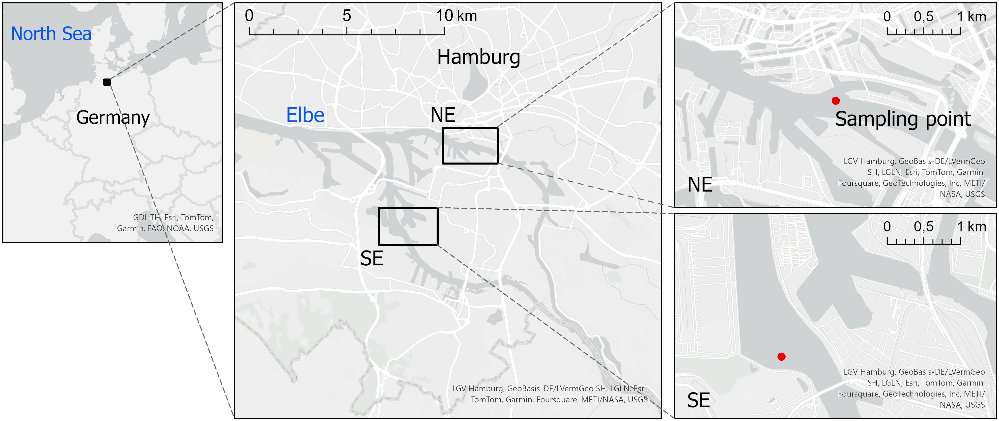
Figure 1 Sampling locations in the “Norderelbe” (NE) and “Suederelbe” (SE).

The sampling device used was a sediment corer developed at the Institute of River and Coastal Engineering (Patzke et al., 2019, 2022). The corer penetrates the upper sediment layers by its own weight and extracts cores with a diameter of 20 cm and a maximum height of 1.20 m. The penetration depth of the corer varies depending on the attached extra weights and the present bed densities. In both campaigns, the corer penetrated about one meter into the bed. In Witt et al. (2023) it was shown that the device is capable of collecting naturally stratified bed samples, thus the properties (grain size distribution, loss on ignition) of the sediment used in this study can be seen as an average of the top one-meter layer of the bed.

2.2 Sediment characteristics

The sediment samples from the two sampling areas exhibit a comparable grain size distribution (GSD) (see Table 1). The GSD was derived by a combined sieve and hydrometer analysis according to DIN EN ISO 17982-4. The clay content (d < 2 μm) of both samples with around 24% is way above the threshold of 5-15% found in literature for dominant cohesive behavior of the sediment (e.g. van Rijn (1993), clay defined as d < 4 μm). In terms of silt (2 – 63 μm) and sand (> 63 μm) content the samples vary slightly with a three percent difference in each case, with the sample from SE showing a higher silt and correspondingly a lower sand content. For both samples, the sand fraction is in the range of fine sand (< 200 μm) only. Consequently, the values for the median diameter D₅₀ and D_{50, mud}, which is defined as the median diameter of the mud-fraction (clay and silt), are comparable. The loss on ignition is higher for sampling site SE (11.5%) than for site NE (8.4%) indicating a higher organic content.

Table 1

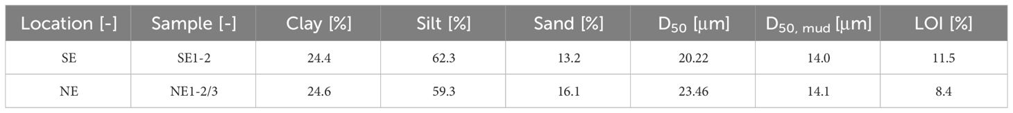
Table 1 Sediment characteristics of the samples used for erosion experiments.

2.3 Erosion experiments

2.3.1 Adapted microcosm system “C-GEMS”

An adapted Gust-Erosion-Microchamber-System (GEMS) was utilized for the erosion experiments. The GEMS was presented in (Gust, 1989) in its original version as an apparatus for generating precisely defined wall shear stresses. To generate wall shear stresses, a disk (with or without a skirt) rotates at a known speed and distance to the sediment surface in a cylinder, which upper part is filled with water. Simultaneously water is pumped out through the center of the disk at a specified rate and eccentrically pumped back into the chamber through the chambers lid. Both the attached skirt and the pumping of the water are supposed to further homogenize the bed shear stress distribution on the sediment surface (Gust, 1989; Gust and Müller, 1997). The GEMS is usually employed as an “open system” (Work and Schoellhamer, 2018; Seo et al., 2020), meaning the water from the erosion chamber is pumped to a turbidity meter and collected as water samples, which are filtrated afterwards to calibrate the turbidity measurements and derive the SSC evolution in the erosion chamber over time. The water, which is pumped out of the erosion chamber, is constantly replaced with new water from a tank with tap or site-specific water. This procedure entails that the SSC in the erosion chamber does not accumulate over the duration of the experiment, but is directly related to the rising and falling of the erosion rate. The main disadvantages of this setup are the high consumption of experimental water and the effort to derive the SSC evolution from turbidity data, since the utilized turbidity probes are usually calibrated based on the determination of the SSC of water samples taken during the experiment. Both of these factors can result in a relatively small number of applied load steps in practice.

The Closed-GEMS (C-GEMS) introduced in Patzke et al. (2022) aims to overcome these restrictions and additionally provides near-natural conditions by allowing the accumulation of suspended sediment over the experimental procedure. In this setup, the water, which is pumped from the erosion chamber, is led to a second chamber, the measuring chamber, where the evolution of the SSC is measured. From the measuring chamber, the suspension is returned to the erosion chamber at the same flow rate, leading to constant volumes in both chambers. In the measuring chamber, an additional pump cycle ensures continuous homogenization of the suspension and prevents the accumulation of sediment particles at the bottom of the chamber. In this study, major optimizations of the C-GEMS are introduced in terms of reduced measurement chamber dimensions and improved SSC-measurements by using a wide-range turbidity sensor.

An outline of the system employed for this study is shown in Figure 2. The erosion chamber has a diameter of 20 cm and the rotating disk is adjusted to a distance of 7 cm to the lutocline. The total volume of water in the system is ~9.2 liter, of which ~2/3 are contained in the measuring chamber and ~1/3 in the erosion chamber. A larger inner volume of the system would lead to a higher total capacity for suspended sediments until the maximum practicable concentration is reached and therefore might allow longer experimental runs, but would also lead to a rising time lag in recording the change in SSC due to the volume’s buffer effect. The chosen volume has proven to offer a reasonable compromise between these opposing attributes. For the SSC-measurement in the measuring chamber a precalibrated Hach^® Solitax hs-line sc probe, working on a combined infrared absorption scattered light technique, is utilized with a nominal measuring range from 0 – 150 g/l. During the experiments, the density in the measuring chamber is measured with an Anton Paar DMA 35 density meter at least once per load step to check and if necessary, adjust the calibration of the SSC probe.

Figure 2

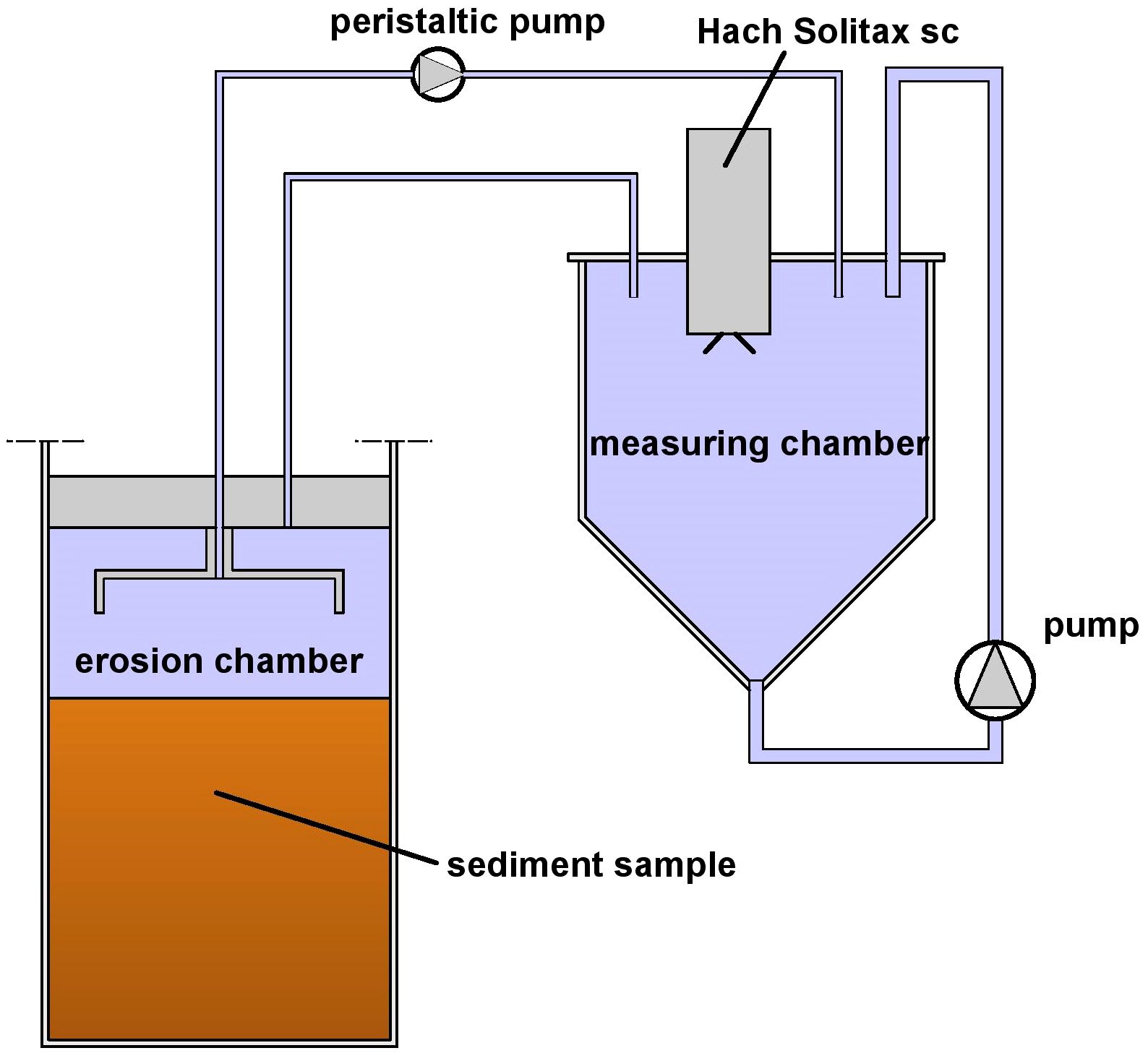
Figure 2 Schematic outline of the utilized adapted Closed Gust Erosion Microcosm System (C-GEMS).

For the experiments two C-GEMS of similar construction and dimensions, but slightly different pump rates were used. The usage of two different pump rate setups was due to the availability of these devices and had no further cause in the experimental design. The applied shear stress velocity and pump rate for the low pumping setup (setup 1) are related to the stirring disk evolutions as follows: (Equations 5, 6)

$\begin{array}{ll}{u}_{\ast }=-\mathbf{2.07}\ast {\mathbf{10}}^{-\mathbf{5}}{n}^{\mathbf{2}}+\mathbf{1.57}\ast {\mathbf{10}}^{-\mathbf{2}}n+\mathbf{0.10527}& (5)\end{array}$

$\begin{array}{ll}Q=-\mathbf{0.0318}{n}^{\mathbf{2}}+\mathbf{5.5}n+\mathbf{20}& (6)\end{array}$

with u_* as shear stress velocity [cm/s], stirrer revolutions n [1/min] and pump rate Q [ml/min]. The applied bed shear stress τ_b is calculated as ${\tau }_b=u_{*}^2\ast {\rho }_w$. For the calculation of τ_b, the increase of the density of the suspension above the sediment surface over the experimental duration due to the increasing SSC is neglected, since the influence is sufficiently small (mostly < 1%). Setup 2 worked on higher pumprates (factor 1.5) resulting in higher shear stresses (factor 1.22).

2.3.2 Sample preparation and experimental procedure

In total 34 erosion experiments with homogenized samples and bulk densities from 1050 – 1250 kg/m³ have been conducted. For sediment from sampling location SE densities from 1050 – 1200 kg/m³ were tested, whereas for NE-sediment the range from 1100 to 1250 kg/m³ was covered. For both locations steps of 25 kg/m³ were applied (see Table 2). The structural density, which is defined as the density at the gelling point, where an interconnected matrix of solids has formed (see Winterwerp et al. (2021)), for sediment from location SE was determined as ~1080 kg/m³ from previous settling column experiments, thus densities 1050 kg/m³ and 1075 kg/m³ are slightly below the structural density. The full range of tested densities covers the in-situ measured densities of the top 50 cm layer of the sediment bed at location SE (Witt et al., 2023).

Table 2

Table 2 Overview of conducted experiments and tested wet bulk densities for the two sampling sites, numbers indicate amount of repetitions.

The raw sediment samples were thoroughly homogenized before being partially filled into the erosion chamber. In the chamber, the samples were diluted with site-specific water (ρ_w=998 kg/m³) to the desired density and homogenized again. The desired density was set with an accuracy of ±1 g/l and was repeatedly checked with an Anton Paar DMA 35 density meter. The final sediment layers had a height of 6 – 12 cm depending on the density of the diluted sample (lower height for high densities due to lower expected erodibility). Then, site-specific water was added on top of the sediment-mixture to the chamber. This process had to be carried out very carefully and slowly (~15 minutes for 3 l of water) to minimize the disturbance of the sediment surface. The top-part of the C-GEMS (consisting of lid, stirring plate and a height adjustment system) was attached and the stirring plate was adjusted to the correct height in relation to the sediment surface. The last step was to fill the measuring chamber with site-specific water and start the pump cycles. One hour after the last homogenization of the samples the erosion experiments were started (except experiments with densities 1050 kg/m³ and 1075 kg/m³ with only 0.5 hours in between to reduce settling effects due to density below the structural density).

During the experiments, a maximum of 13 load steps of 0.028 - 0.33 N/m² (setup 1) respectively 0.034 – 0.40 N/m² (setup 2) were applied with a load step duration of 15 minutes. At the beginning of each load step, the distance between the sediment surface and the stirring plate was checked and adjusted if necessary. When an SSC of approximately 15 g/l was reached during the experiment, the experiment was terminated because of the increasing non-Newtonian flow behavior of the fluid.

2.3.3 Data processing

The SSC in the measuring chamber was recorded with the Hach^® Solitax sc at 5-second intervals. The measured SSC values were corrected by the background SSC measured at the beginning of the experiment, typically lying in the range of 10 – 30 mg/l. Therefore, the further used SSC values describe the rise in SSC in relation to the initial concentration. To reduce scatter in the data, a moving average of 60 s was calculated for further processing of the data. For one experiment with sediment from site NE, setup 2 and ρ=1250 kg/m³ the data of six load steps had to be excluded due to problems with the pump, which circulates the suspension in the measuring chamber.

Erosion rates ε were derived from the processed SSC data by relating the change in measured SSC at two consecutive time steps to the time interval $\Delta t$, the total fluid volume V_f and the area of the sediment surface A_s (Equation 7):

$\begin{array}{ll}\mathit{\text{ε}}=\frac{(SS{C}_t-SS{C}_{t+\Delta t})\ast V_f}{\Delta t\ast A_s}& (7)\end{array}$

2.3.4 Methods to determine τ_c

Two methods to determine the erosion threshold τ_c have been utilized and compared. In both cases τ_c is defined as the surface erosion threshold, implying that small erosion rates might also occur at shear stresses below τ_c due to erosion of single flocs (c.f. Winterwerp et al. (2021)). The two methods are:

● Log-log regression of mean erosion rates per load step vs. applied bed shear stress τ_b. The erosion threshold τ_c is determined as the interpolated shear stress at the intercept of the regression with ε_f=1 x 10^-5 kg/(m²s), as an extrapolation to zero erosion is not possible. The floc erosion rate ε_f is defined as the value of ε at τ_b–τ_c = 0, meaning at zero excessive shear (background erosion rate) (Parchure and Mehta, 1985). Parchure and Mehta (1985) evaluated ε_f for different mud samples and despite some variation in the derived magnitudes, the utilized value of ε_f=1 x 10^-5 kg/(m²s) in Amos et al. (2003) is seen as a practical choice.

● Log-log regression of mean SSC per load step vs. applied bed shear stress τ_b. The value of τ_c is determined as the interpolated shear stress of the regression with SSC_T=40 mg/l. The threshold describes the accumulated eroded mass over all prior load steps and was set to this value based on an analysis showing a good correspondence with the value of ε_f used for method one. An extrapolation to zero SSC is again not possible, due to log space. Solving for background SSC, without prior correction of the measured SSC by this value, would be possible, but would lead to very low derived τ_c values because the highly sensitive SSC-probes detect an increase in SSC usually even during the first load step (background- or floc erosion). The value of SSC_T=40 mg/l can be generalized and adapted to devices with other dimensions by relating it to the fluid-volume and sediment-surface area of the GEMS system, leading to a total eroded mass of 0.37 g and ~13 g/m² respectively. Though the chosen SSC-threshold is seen to be dependent on the load-step duration and might need calibration for varying values.

For both methods, all data points were used for the respective regression. No further distinction between erosion modes and the point of transition between them was applied to limit the parameters to be set.

3 Results

3.1 Evolutions of suspended sediment concentration and erosion rate

For all conducted experiments the SSC evolution in the measuring chamber was captured and the corresponding erosion rates were derived (see sections 2.3.2 and 2.3.3). In Figure 3 the results for both the SSC and the erosion rates for three different exemplary bulk densities (1100, 1150 and 1200 kg/m³) for the two sampling sites SE and NE are shown. The chosen densities represent the range of tested densities for which data from both sampling locations is available and illustrate the observed trends and relationships. The figure gives an impression of the generally high repeatability of the SSC measurements and erosion rate calculations, especially when considering the rapid change of erodibility with increasing bulk densities of the sediment mixture.

Figure 3

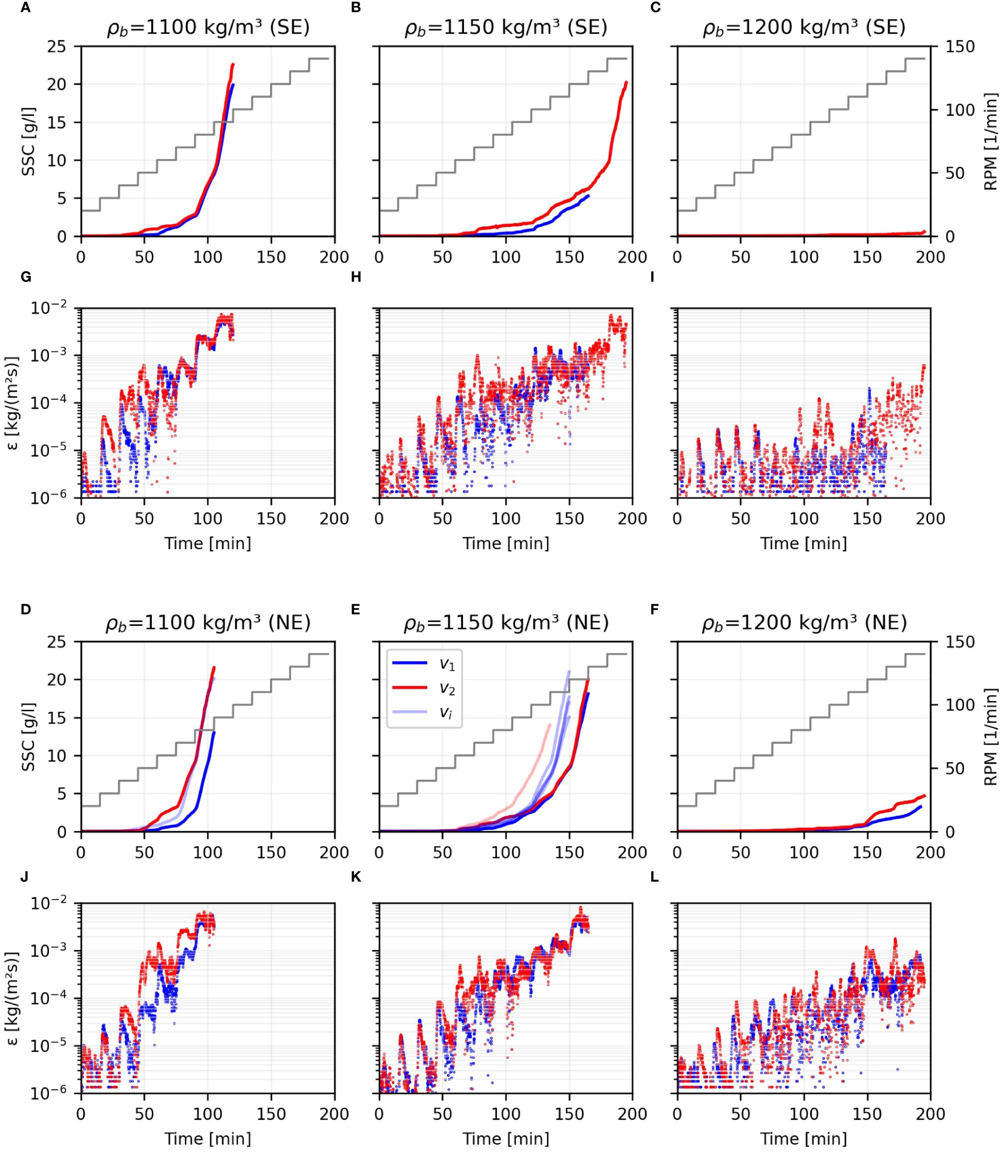
Figure 3 Exemplary evolution of SSC and ε for experiments with bulk densities of 1100, 1150 and 1200 kg/m³. (A–C) show the SSC evolution for SE-experiments, (D–F) show SSC for NE-experiments. (G–L) show the ε-evolution for SE resp. NE. Only highlighted regimes (initial runs v₁ and v₂) are shown in ε-plots for better readability. Additional runs (v_i) shown in low opacity. Color indicates C-GEMS setup 1 (blue) and setup 2 (red). Revolutions per minute (RPM) are displayed on secondary y-axes instead of τ_b because the two C-GEMS setups worked on identical RPM regimes, but slightly different τ_b steps (see end of section 2.3.1).

Focusing on the SSC plots against experimental time (panel (A)-(C) for SE and (D)-(F) for NE) the strong relationship between ρ_b of the samples and the observed SSC evolution becomes evident. For sediment from SE at ρ_b=1100 kg/m³ the first increase in SSC on the applied linear scale becomes visible at around minute 50 and the curve rises quickly over the following load steps to reach values of 20 g/l after 120 minutes duration. The SSC evolutions for ρ_b=1150 kg/m³ and ρ_b=1200 kg/m³ exhibit a consistent shift to the right, meaning a longer experimental duration and thus higher applied bed shear stresses are needed to cause a similar SSC-increase. For ρ_b=1200 kg/m³ the SSC reaches values of < 1 g/l after the maximum duration of 3.25 h. The decreasing erodibility with rising bulk densities of the slurry is caused by an increased amount of cohesive particles per volume element and therefore more and stronger bonds between the single particles. Since the samples tested are homogenized and have uniform erosion characteristics over the depth of the sample, the gradient of the SSC curves is theoretically constant for each load step and increases with the applied bed shear stress. This relationship is generally well represented in the measured data, especially for higher applied bed shear stresses.

For load-steps of lower bed shear stresses most of the SSC curves approach a plateau asymptotically. This observation is confirmed by the corresponding plots of ε, which are shown under the SSC-plots (panel (G)-(I) for SE and (J)-(L) for NE). For low τ_b the erosion rates tend to peak at the beginning of each load-step and decrease over the remaining load step duration. This trend in ε-evolution is commonly observed in experiments with density-stratified samples and increasing erosion resistance over the depth of the sample (type I erosion, see section 1). The reason why the described trend is also apparent in the presented experiments, despite working with homogeneous samples, is seen in the fact that during the first load steps only the topmost part of the sample (< 1 mm depth) is eroded. In this top-layer particles are incorporated into the grain structure to varying degrees and therefore exhibit a differing erosion resistance, meaning that the erosion resistance (as also the applied load) follows a probability distribution (Winterwerp et al., 2012). This leads to decreasing erosion rates over the load-step duration, since the number of particles that might get eroded declines. With increasing load and erosion depth, the erosion rates become more and more constant over each load-step and reach values of up to 5 x 10^-3 kg/(m²s).

The setup 2 of the utilized C-GEMS generally records an earlier increase in SSC and ε compared to setup 1, as expected due to the slightly higher τ_b applied. Comparing the results of the two sampling sites SE and NE, the evolution of SSC- and ε indicates a higher erodibility for material from site NE. For example, for ρ_b=1200 kg/m³ the measured final SSC for site SE is < 1 g/l, whereas values of ~4-5 g/l are measured for site NE. For the other densities, this relationship is reflected by faster increasing SSC and erosion rates as well.

3.2 Derivation of erosion thresholds

From the SSC and ε-evolutions, the mean values of the parameters per load-step have been calculated (see section 2.3.4) and are shown in Figure 4 (SE) and Figure 5 (NE) against the applied bed shear stress. Focusing on the exemplary bulk densities for sampling site SE (Figure 4), the diagrams illustrate that for both methods to derive τ_c, the erosion threshold increases together with the bulk density. Additionally, the gradient of the regression lines consistently decreases with increasing bulk density. These fundamental relationships are in line with the observations described in section 3.2 and theory and indicate a lower erodibility for higher bulk densities. For the illustrated densities the erosion rate method leads to values for τ_c of 0.053 – 0.430 N/m². While for bulk densities of 1100 kg/m³ and 1150 kg/m³, this method yields a small semi-range (SR) for calculated τ_c in repetition tests of < 0.005 N/m², the spread of the derived values rises drastically for ρ_b=1200 kg/m³ (SR=0.086 N/m²). Also, the calculated coefficients of determination (R²; calculated based on log-transformed data) indicate a strong linear relation between the applied bed shear stress and ε for bulk densities 1100 kg/m³ and 1150 kg/m³ (R² ≥ 0.94), but drops for ρ_b=1200 kg/m³. The SSC-method yields values for τ_c in the range of 0.060 – 0.159 N/m² and results in small semi-ranges of τ_c in repetition tests (SR < 0.008 N/m²) and high R² values (R² ≥ 0.91) for all three shown bulk densities. Compared to the ε-method the SSC-method leads to slightly higher τ_c values for ρ_b=1100 kg/m³ and ρ_b=1150 kg/m³, but significantly lower values for ρ_b=1200 kg/m³. The reason for the inconsistent results of the ε-method for ρ_b=1200 kg/m³ is seen in the fact that this bulk density is close to the application limit of the utilized C-GEMS devices for sediment from this specific site. Only a small amount of sediment is eroded over the experimental duration, leading to low erosion rates and large scatter in the erosion rate data (see Figures 3, 4). The large scatter in erosion rate data in turn yields low R² values and a large spread in derived erosion thresholds. Since, in contrast to ε, the SSC is accumulating over time, the SSC data exhibits much less scatter and allows a more reliable determination of τ_c even at the application boundary. In the upper part of Table 3, the results for all experiments conducted with material from sampling site SE are summarized. The data derived in the additional experiments underlines that both applied approaches yield comparable values for τ_c, SR and R², except at the upper application limit where the SSC-method is superior to the ε-method.

Figure 4

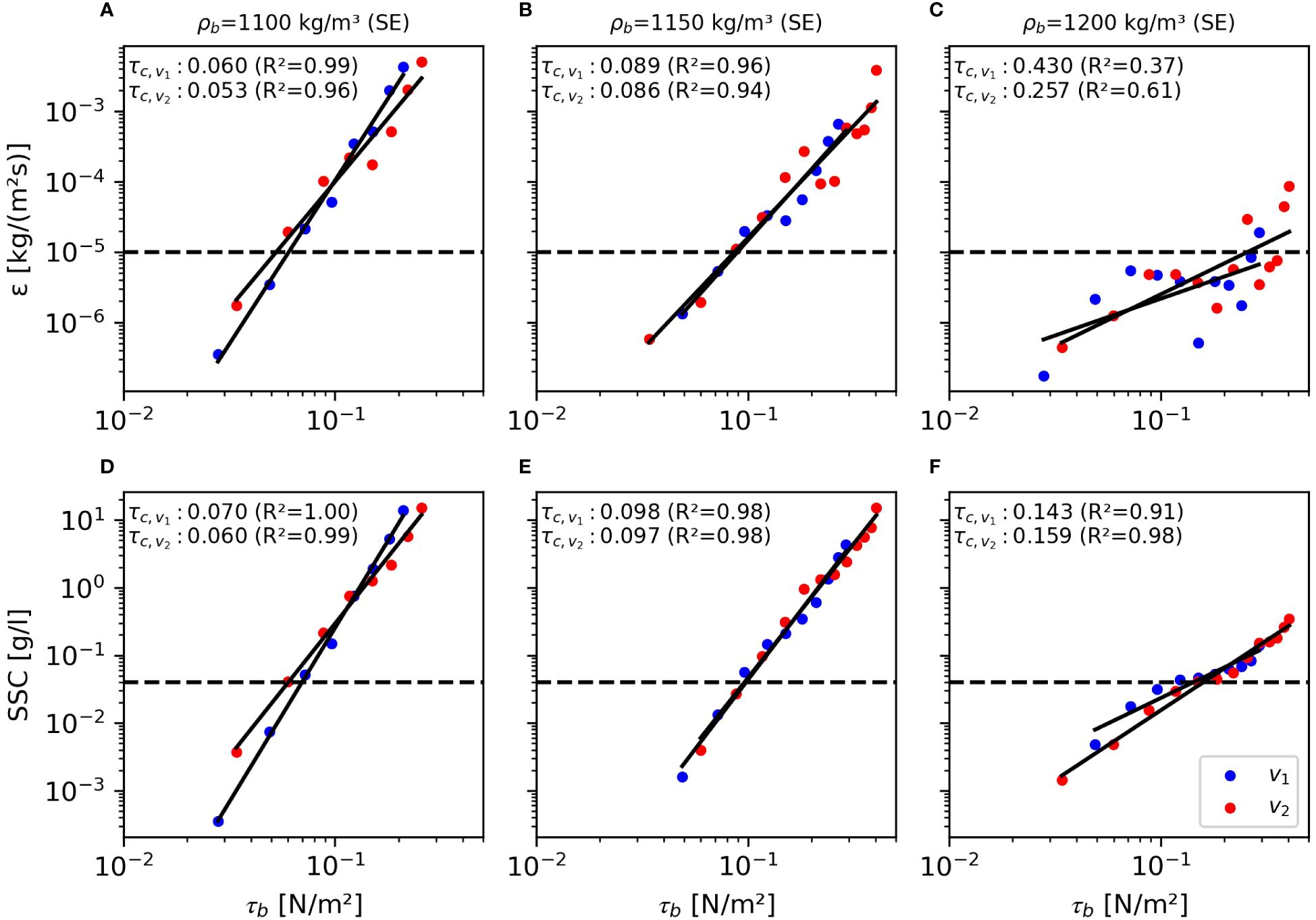
Figure 4 Log-log-regression of ε/SSC against τ_b and derived values for τ_c for sampling location SE (exemplary bulk densities 1100, 1150, 1200 kg/m³). (A-C) show results for ε-method, (D-F) show results for SSC-method. For the initial two experiments (v₁, v₂) the regression lines and calculated values for τ_c are highlighted and the data from additional runs (v_i, if conducted) is shown in low opacity and without regression lines for better readability.

Table 3

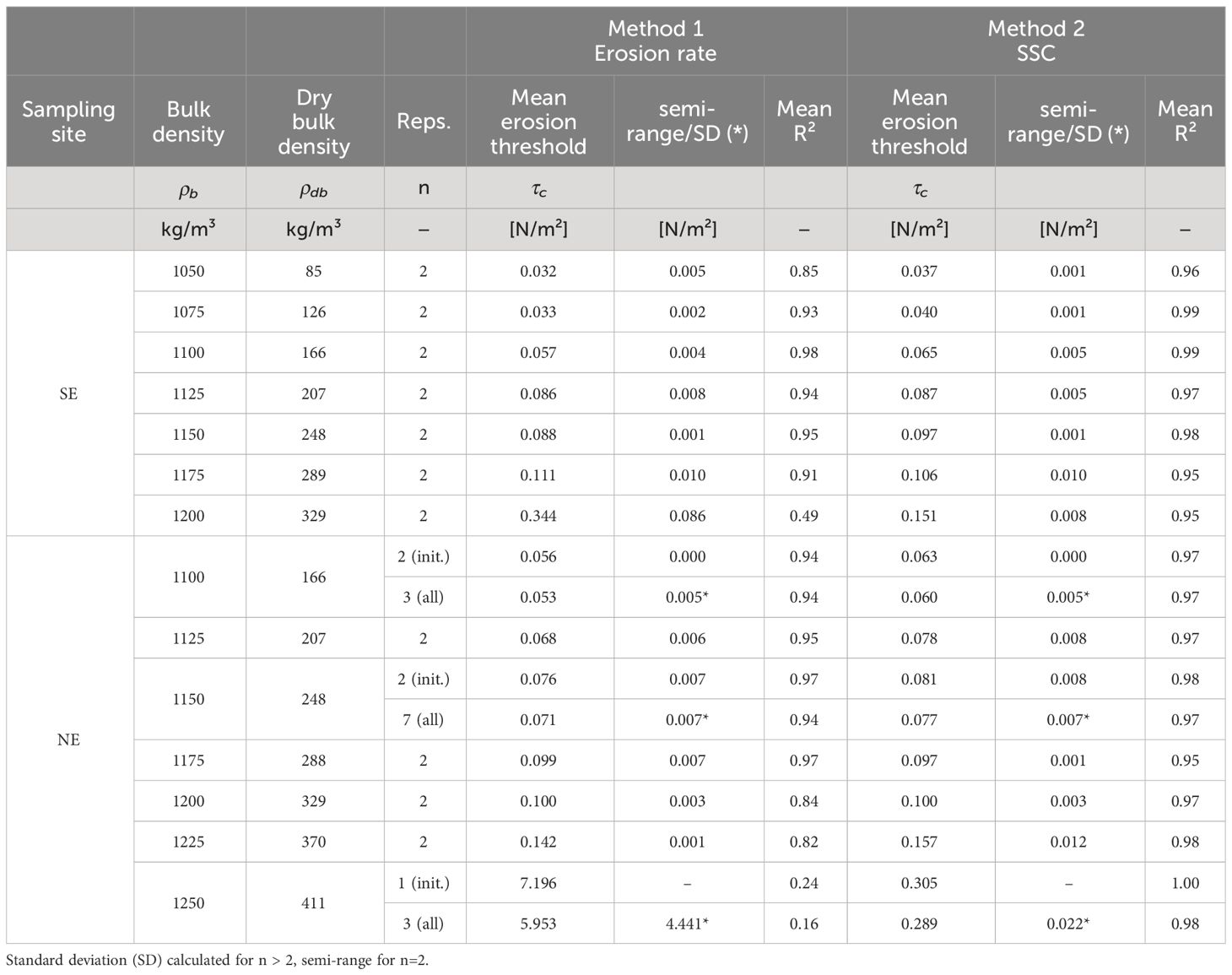
Table 3 Summary of derived mean erosion thresholds for all tested densities for both sampling locations with ε- and SSC-Method.

The described trends and relationships are also valid for the experiments conducted with sediment from site NE. The results for the three exemplary bulk densities are illustrated in Figure 5 and the data for all experiments is summarized in the lower part of Table 3. As expected from the data shown in Figure 3, the erosion thresholds derived for site NE are generally lower than for site SE. The higher erodibility of the NE-sediment also leads to a shift of the application limit of the GEMS device to higher bulk densities. While for SE sediment for ρ_b=1200 kg/m³, only the SSC-method yielded reasonable results, for sediment from site NE the ε-method was still applicable for this bulk density as well. The application limit was reached at ρ_b=1250 kg/m³ for site NE, where the ε-method again led to unreasonably high values for τ_c, a high spread of the derived values and low R².

Figure 5

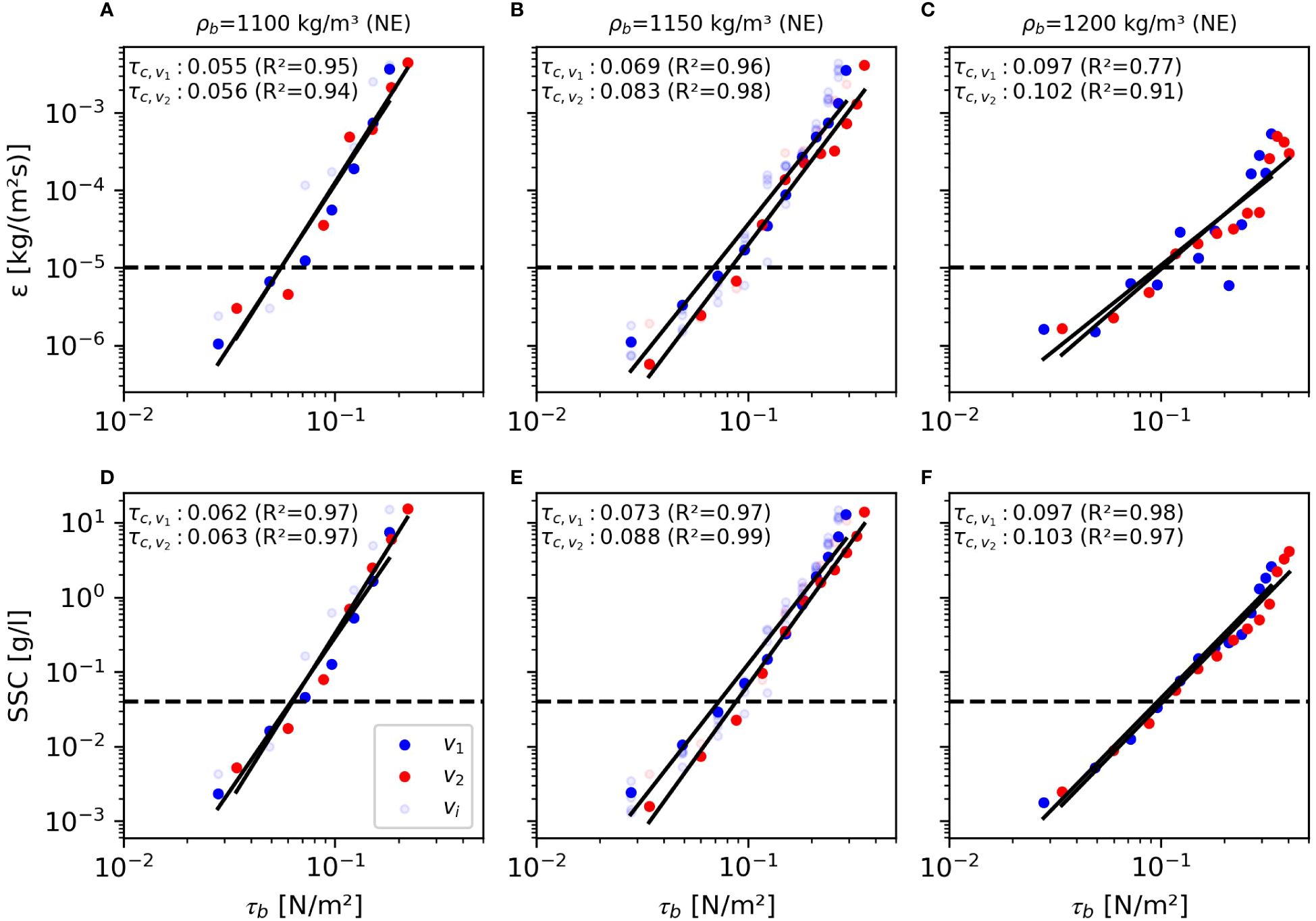
Figure 5 Log-log-regression of ε/SSC against τ_b and derived values for τ_c for sampling location NE (exemplary bulk densities 1100, 1150, 1200 kg/m³). (A-C) show results for ε-method, (D-F) show results for SSC-method. For the initial two experiments (v₁, v₂) the regression lines and calculated values for τ_c are highlighted and the data from additional runs (v_i, if conducted) is shown in low opacity and without regression lines for better readability.

For NE-sediment with ρ_b=1100 kg/m³, ρ_b=1150 kg/m³ and ρ_b=1250 kg/m³ additional experiments have been conducted to check and quantify the repeatability of the experimental setup and approaches to derive τ_c. The additional repetitions were conducted around one month after the initial experiments, which were carried out in the first two weeks after the measurement campaign. In the additional experiments, slightly lower values for τ_c were derived. While the SSC-method for ρ_b=1150 kg/m³ in the initial experiments yielded a mean τ_c of 0.081 N/m² (SR=0.008 N/m², n=2), for the additional repetitions a mean of 0.075 N/m² (SD=0.005 N/m², n=5) was derived, leading to an overall value of 0.077 N/m² (SD=0.007 N/m², n=7) (see Table 3). The measured change might be caused by a change in sediment properties evoked by biological activity. However, due to the relatively small database and small measured changes in τ_c, this is only an assumption yet and needs further investigation.

The two methods used to derive τ_c delivered comparable results for most of the bulk densities tested, with a small spread in derived values in repetition tests and strong linear correlation (in log-space) between applied bed shear stress and measured SSC/ε (slightly higher for SSC-method). Especially because of the better performance of the SSC-method at the upper limits of application, this method should be preferred though and the data derived by this method is used to fit models for τ_c in section 3.3. To investigate the influence of the applied values of the thresholds for SSC (SSC_T) and ε (ε_T) on the derived values for τ_c, a sensitivity analysis was conducted using the example of site SE (Figures 6A, B). The chosen thresholds were varied by ±50%. As expected from the decreasing slope of the regression lines with increasing bulk density (Figure 4), the total variation of the derived τ_c also increases with ρ_b. Especially for the lower and middle values of the tested density range, the variation is relatively small, e.g. for SSC-method and ρ_b=1150 kg/m³ the variation of SSC_T of ±50% leads to a change in the derived τ_c of +10.6% and -15,7%, respectively. Figure 6C additionally shows an analysis of the influence of different time periods (t_av) over which the average value of ε is calculated for each load step when using the ε-method. A value of t_av=5 min means only the first five minutes of each load step were used for averaging. This analysis can be interpreted as the expected sensitivity of the calculated τ_c with respect to a corresponding change in load step duration. Since the magnitude of ε decreases significantly over the applied load step duration for load steps of lower τ_b (see Figure 3), a shortening of t_av leads to higher calculated averages of ε and consequently to a decrease of the derived values of τ_c. For the SSC-method, a similar analysis is not feasible based on the dataset, since this parameter accumulates over the duration of the experiment und thus the actually applied load step duration directly influences the SSC in subsequent load steps.

Figure 6

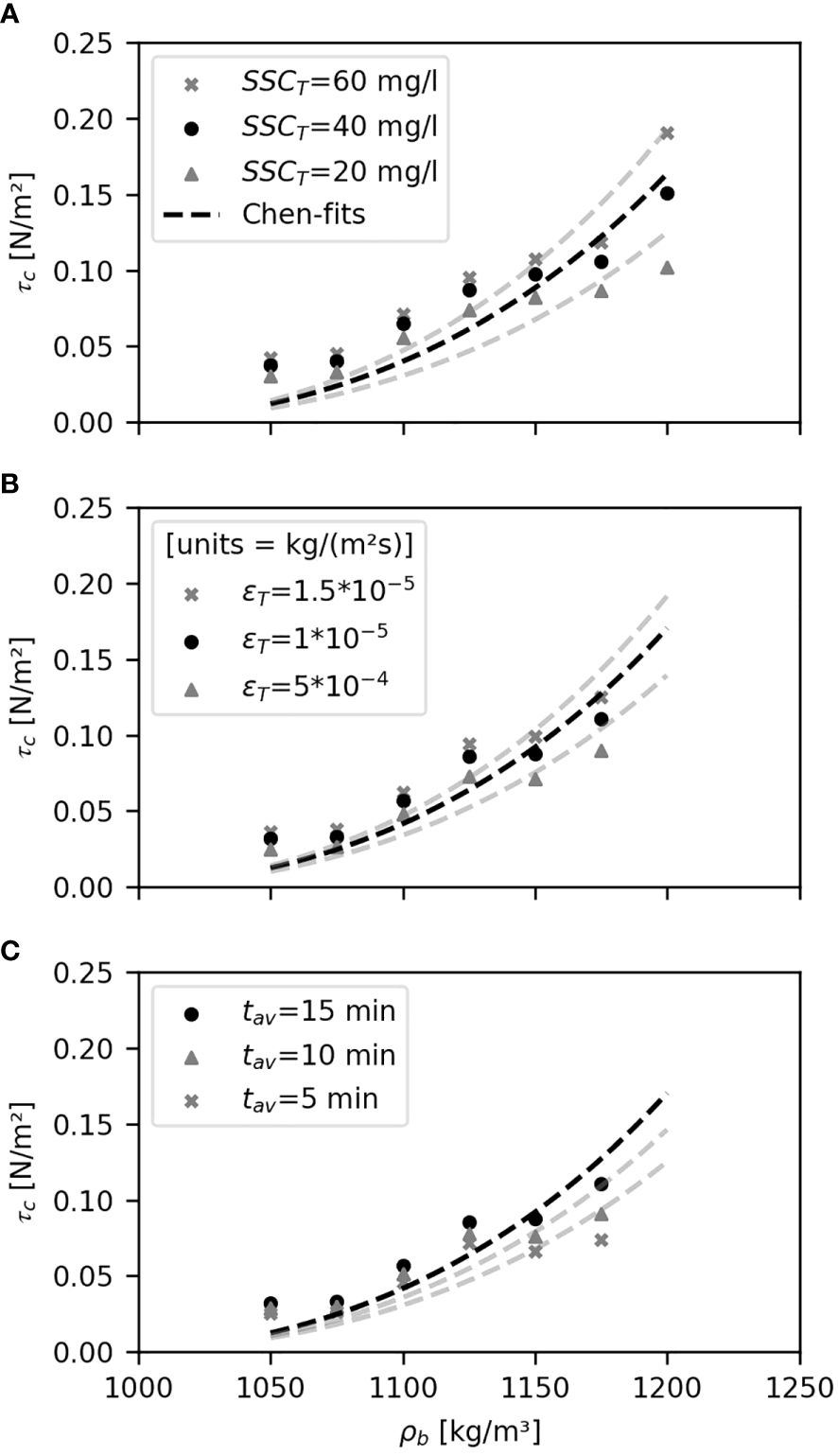
Figure 6 Sensitivity analysis of the calculated values for τ_c and parameter A of the Chen-model with respect to the thresholds for SSC (SSC_T) and ε (ε_T) and the time periods over which the average value of ε is calculated for each load step (t_av), using the example of site SE. (A) shows the results for varying SSC_T using the SSC-method, (B) for varying ε_T using the ε-method and (C) for varying t_av using the ε-method. For ε-method ρ_b=1200 kg/m³ is excluded.

Summaries of τ_c derived from field and laboratory experiments in other studies can be found in Debnath and Chaudhuri (2010) and Houwing (1999). As stated in section 1, the derived values are strongly influenced by the erosion device used, the specific sediment properties and the applied definition of the erosion threshold. There is only a limited amount of data available for bulk densities in the range that was tested in this study. However, the studies from Righetti and Lucarelli (2007), who tested benthic lake sediments with bulk densities from 1025 – 1175 kg/m³ in a Sedflume and derived values for τ_c in the range of 0.01 – 0.23 N/m², and Amos et al. (1997), who worked with mud flat sediments with ρ_b from 787 – 1273 kg/m³ in a Sea Carousel and derived values for τ_c of 0.15 – 0.5 N/m², show that the findings in the present study are well covered by the observations in previous studies.

3.3 Model application

The data on τ_c derived by SSC-method in section 3.2 is used to fit two mathematical models. The first model is a power-law relation between ρ_db and τ_c (Equation 1) and the second model is a more complex and physically based model shown in Equation 3, proposed in Chen et al. (2021). The application of both models requires the calculation of ρ_db as shown in Equation 2. From the assumed density of the particles of the mud-fraction ρ_pm=2575 kg/m² (cf. Malcherek (2010)) and sand particles (ρ_pps=2650 kg/m³) the weighted particle density for the sediment mixture is calculated as ρ_s = ρ_ps + ρ_pmP_m. The derived values for ρ_db are shown in Table 3. In Figure 7 the fitted models are illustrated. Both models have been fitted to the data obtained from the two sampling sites separately and additionally to the whole dataset using least-squares method. For site NE only the derived data from the initial two experiments (one in case of ρ_b=1250 kg/m³) was used, even if more repetitions have been carried out, due to the unclear effect of the time span between the experiments (see section 3.2). The obtained fit parameters and the resulting root mean squared errors (RMSE) are summarized in Table 4.

Figure 7

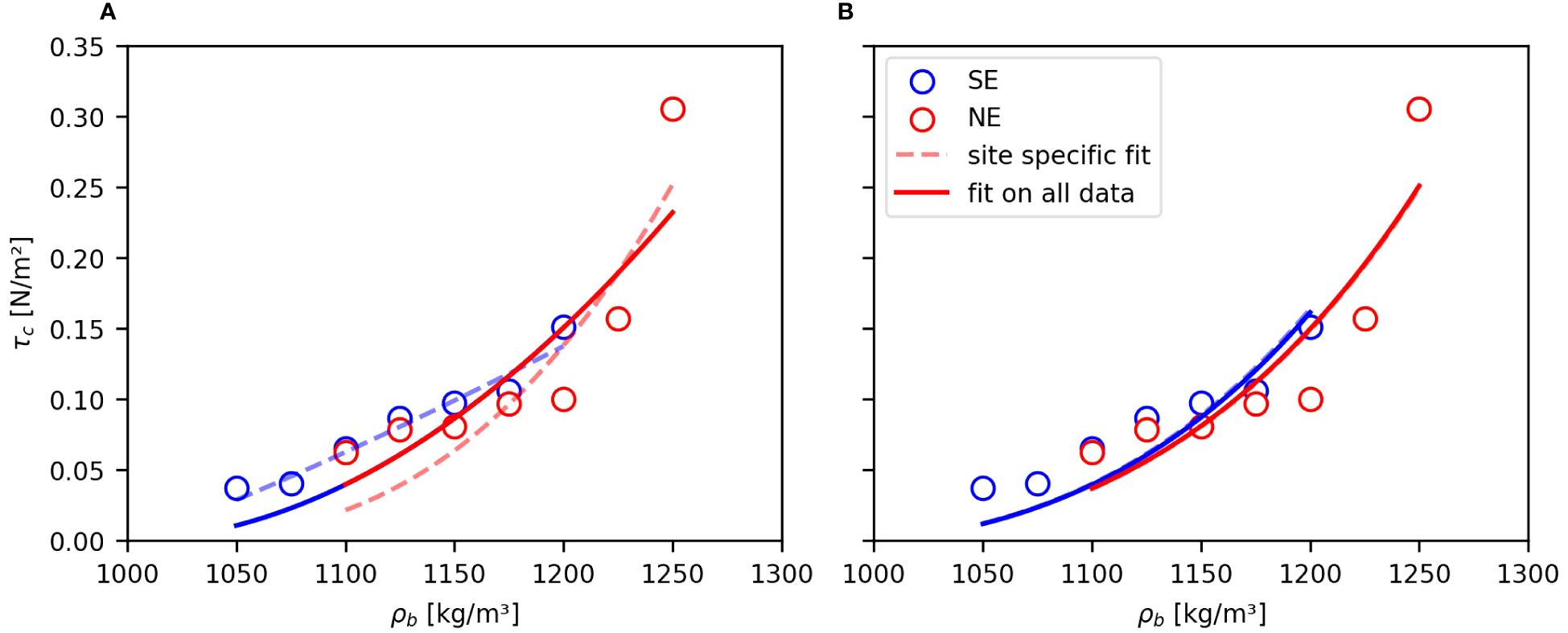
Figure 7 (A) Power-law fit of τ_c, (B) Fit of Chen-approach for τ_c (both shown against bulk density). Dashed lines indicate fits of SE/NE data based on respective datapoints only. Solid lines indicate fit of SE/NE data based on fit parameters derived from whole dataset (in (B) the dashed lines are fully covered by the solid lines).

Table 4

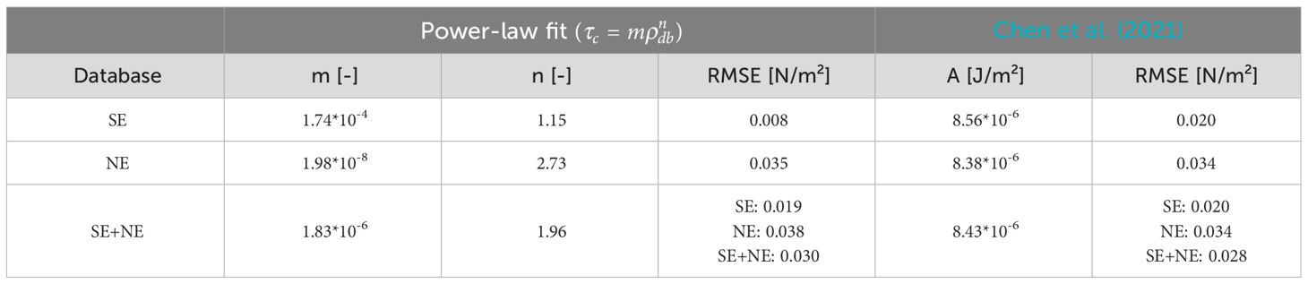
Table 4 Derived fit-parameters for the applied mathematical models.

The power law-fit for site SE suggests an almost linear increase of τ_c over the considered range of bulk densities (exponent n=1.15) while for site NE the power-law relation is more distinct. However, the derived model for NE underpredicts the erosion thresholds in the lower range of ρ_b=1100 – 1150 kg/m². Fitting the model on the whole dataset (SE+NE) yields a reasonable model for the whole considered range of densities and both sampling sites. The derived fit-parameters for this model are m=1.83 x 10^-6 and n=1.96. Earlier investigations, which were carried out by Owen (1975) and Thorn and Parsons (1980) (see see Zhu et al. (2008)) with remolded sediment samples from four different estuaries, led to values for m of 6.85 x 10^-6 resp. 5.42 x 10^-6 and values for n of 2.44 resp. 2.28. An extensive overview of derived fit-parameters from other studies carried out with different muds and erosions devices can also be found in Schweim (2005), with m ranging between 2.5 x 10^-8 – 1.5 x 10^-2 and n between 0.73 – 2.44. Although the fit-parameters derived in this study are comparable to earlier studies, their values vary significantly with the underlying dataset both for this study and earlier works.

The model proposed in Chen et al. (2021) includes only a single fit-parameter, denoted as A (units J/m²). Additional sediment properties used to fit the model are shown in Table 1. The mud-fraction is calculated as the sum of clay and silt fractions and for parameters ρ_ps and ρ_pm the same assumptions are made as described for the power-law model. The derived values for the fit parameter A are 8.56 x 10^-6 J/m² based on SE-data and 8.38 x 10^-6 J/m² based on NE-data. The fit on the whole dataset yielded A=8.43 x 10^-6 J/m². It stands out that the fit-parameters show only a marginal spread. In Chen et al. (2021) the authors applied the model to multiple natural muds from different locations and concluded that the value of A is generally in the order of 10^-6 or 10^-5 J/m² and specifically for natural mud and sand-mud mixtures in the range of 2.86 x 10^-6 – 1.04 x 10^-5 J/m² (if no field data is available the authors propose a general value of A=3.97 x 10^-6 J/m²). The values for A derived in this study are covered well by the findings of the authors, lying close to the mean of A-values determined by them. The small spread in A suggests that the consideration of the physical parameters describing the mud-fraction of the sediment leads to a more profound model than the power-law model also applied, relating the evolution of τ_c to the actual sediment properties and leaving a lower degree of freedom for the empirical fit. Figure 7B additionally shows that the slightly lower erosion thresholds for NE-sediment might be at least partly caused by the (also slightly) different grain size distribution, since the same fit-parameter (solid lines) leads to lower τ_c values. The lower spread of A is also reflected in the calculated RMSE. While for the power-law fit the RMSE rise considerably for both individual sites when the model is fitted on the whole dataset and not on the site-associated data only, for this model, the RMSE is almost independent of the chosen database for the model fit (see Table 4). A comparison of the RMSE of the two different models fitted on the whole dataset additionally reveals a slightly better adaption of the Chen-model to the measured erosion threshold data overall. A sensitivity analysis conducted for the value of the fit-parameter A with respect to the applied values of SSC_T and ε_T, using the example of site SE (fitting lines shown in Figures 6A, B), shows that a variation of the values of ±50% leads to a range of A of 7.30 x 10^-6 – 1.0 x 10^-5 J/m² for ε-method and 6.54 x 10^-6 – 1.01 x 10^-5 J/m² for SSC-method. The analysis of different time periods t_av used for averaging ε for each load step when using the ε-method (Figure 6C) shows that the applied reduction of t_av from 15 to 5 min leads to a range of A of 6.55 x 10^-6 – 8.91 x 10^-6 J/m². Despite the applied variation of SSC_T, ε_T and t_av the derived values for A are well covered by the expected range of A, accordingly.

4 Discussion and summary

4.1 Discussion

Some additional considerations regarding the results obtained and the experimental procedure are discussed in this section. Since the C-GEMS is a closed system and the eroded sediment accumulates throughout the duration of the experiment, the question arises, as with all closed erosion devices, whether deposition occurs simultaneously with erosion. In general, two concepts to describe the onset of deposition of cohesive sediment exist: i) the existence of a critical shear stress for deposition τ_d, which is lower than τ_c, meaning deposition and erosion are mutually exclusive (Krone, 1962; see Whitehouse et al. (2000)) and ii) the assumption that deposition occurs continuously also at higher shear stresses (see e.g. Winterwerp et al. (2021)). While modeling of in-situ data may yield better results under the assumption of continuous deposition, many laboratory studies have demonstrated the existence of a critical shear stress, below which deposition does not occur (see Sanford and Halka (1993)). This discrepancy may be due to differences in scale and turbulence conditions and the absence of still water/flocculation periods in laboratory experiments. In the C-GEMS, the turbulent mixing in the erosion chamber is supported by the constant suction and feeding of the suspension and flocculation of eroded particles is hardly possible because the particles are exposed to high shear rates in the different pumping cycles, resulting in very small floc sizes and (theoretical) settling rates. Both of these factors would significantly harm deposition. Even if these flocs/particles briefly were to come into brief contact with the sediment surface it is not unlikely that they would be able to withstand the applied bed shear stress, so they would be immediately eroded again. Nevertheless, we cannot completely rule out the presence of deposition during the experiments, so the derived erosion rates can be interpreted as net erosion flux.

In section 3.3 it was shown that the Chen-model can explain the observed higher erodibility of sediments from site NE at least partly with the sediment composition (cf. Figure 7B), slightly lower predicted τ_c for NE-sediment for the same value of A). To make a statement whether this is the only reason for the noticed difference in erodibility or if other reasons e.g., a difference in the kind of organic matter, influence the erosion behavior, further investigation is needed. Focusing on the fit-parameter A, in Chen et al. (2021) it is stated that the value of A is supposed to be site-specific because it describes the bed surface roughness and the cohesion strength, which is, among others, influenced by the mineral composition of the sediment and the pore water environment. Since the sampling sites investigated in this study are only a few kilometers apart and comparable in characteristics, it seems plausible to assume a broad agreement in characteristics. This assumption in turn leads to the expectation, that the derived parameters for A are in the same range for both sites, as demonstrated in this study.

Another noteworthy point is that the lowest bulk densities tested for site SE (ρ_b=1050 kg/m³ and 1075 kg/m³) are below the structural density (as stated in section 2.3.2). Despite the adjusted, shortened time between sample preparation and the beginning of the erosion experiment for these densities, the onset of the settling process presumably led to higher densities below the lutocline than initially set. The increased densities might have led to an overestimation of the erosion threshold from the conducted measurements and explain the underprediction of τ_c for these bulk densities by the models.

Looking at the applied techniques to derive τ_c, erosion rate and SSC method, the chosen values for the thresholds of ε and SSC are obviously debatable. However, no other method to derive τ_c is available that does not include either defined threshold values, the differentiation of erosion-modi or the definition of erosion/no-erosion states. Indeed, the implementation of a kind of threshold (that is always arguable) is imperative, since with highly sensitive sensors even at very low applied bed shear stresses measurable erosion rates can be detected (as shown in this study), which rather result from particle/background erosion than from surface erosion. This observation rises the question if a single value for τ_c is a reasonable concept to describe the initiation of motion of cohesive sediment. However, since most the erosion models in use depend on this type of data, the practical benefits are beyond doubt. Some models (e.g. Parchure and Mehta (1985)) also incorporate the unsharp initiation of motion. The benefit of the tested methods in this work in deriving these data is, that only one single SSC-/ε-threshold is used and that the thresholds are transferable to other devices straightforward, which is hoped to contribute to better comparability of derived erosion thresholds of future investigations.

4.2 Summary

In this work, an improved version of a closed microcosm system (C-GEMS) proposed in Patzke et al. (2022) is presented. The device is used to perform erosion experiments with freshly deposited cohesive sediments collected from two sites on the River Elbe in the area of the Port of Hamburg. For the erosion experiments, the sediments were homogenized and diluted to bulk densities from 1050 – 1250 kg/m³, which is the observed range of bulk densities in earlier investigations over the top layer of the sediment bed (multiple ten-centimeters to about one meter). During the experiments a maximum of 13 load steps were applied with increasing bed shear stresses from 0.028 to 0.33 N/m² (setup 1) resp. 0.034 – 0.40 N/m² (setup 2). The evolution of SSC in the measuring chamber of the C-GEMS was recorded using a Hach^® Solitax sc probe and the corresponding erosion rates were calculated from the change in SSC over time. The results of the SSC- and ε-evolutions indicate a distinct relationship between the bulk density of the cohesive sediment-mixture and the erodibility and exhibit good repeatability. The further investigations focused on the derivation and quantification of the surface erosion thresholds. Two methods were applied for this purpose: i) interpolation of the log-log-regression of mean erosion rates to the threshold value of ε=1 x 10^-5 kg/(m²s) and ii) interpolation of the log-log-regression of mean SSC to the threshold value of 40 mg/l. The derived values for τ_c for both methods showed a good agreement for the considered range of bulk densities except at the upper application limits of the utilized C-GEMS device, where only the SSC-method yielded reasonable results due to significantly lower scatter in the SSC-data compared to ε-data. The reason for the lower scatter of the SSC-data is seen in the accumulating nature of this parameter, as the C-GEMS is a closed system. Comparable studies with other erosion devices support the conclusion that deriving erosion thresholds based on an accumulating parameter leads to more robust results (Amos et al., 2003; Ha and Ha, 2021). Because of the better performance at the application limits it’s suggested that the SSC-method should be preferred over the ε-method when working at the application limits of the device. The derived mean τ_c for location SE (ρ_b=1050 – 1200 kg/m²) with SSC-method are in the range of 0.037 – 0.151 N/m² and for location NE (ρ_b=1100 – 1250 kg/m²) in the range of 0.063 – 0.305 N/m². For NE-site with ρ_b=1150 kg/m³, a total of seven repetitions has been carried out yielding a mean τ_c of 0.077 N/m² with a standard deviation of 0.007 N/m², underlining the reproducibility of the utilized experimental procedure. In a last step the derived τ_c-data was used to fit two mathematical models, a power-law relationship between dry bulk density and τ_c and a model proposed in Chen et al. (2021). The fitting of the power-law model showed a strong dependency of the derived fit-parameters on the respective data used for the fit (SE, NE or SE+NE), while the fitting of the Chen-model yielded practically the same value for the fit-parameter A independent of the chosen database. Using the whole dataset to fit the models, the power-law fit yielded values of the prefactor m=1.83 x 10^-6 and the exponent n=1.96. The fitting of the Chen-model on the whole database led to A=8.43 x 10^-6. All derived fit-parameter are well-covered by the range of values reported in previous studies. Since the Chen-model relates the change in τ_c to the physical properties of the sediment mixture, shows a better adaption to the measured data and the value of the fit-parameter is stable independently of the underlying data subset, it’s concluded that the model is more profound and should be preferred over the highly empirical power-law model.

4.3 Outlook

In further investigations, different models for the erosion rate will be applied to the collected data. Taking the derived relationship between ρ_b and ε for the examined samples into account, the often used linear model based on the work of Partheniades (1965) (see McAnally and Mehta (2000)) reading ε = m(τ_b-τ_c) for τ_b > τ_c, with m as erosion constant, presumably allows only an unsatisfactory adaption to the collected data. In combination with in-situ measured density profiles the derived relations of τ_c and ε enable the generation of depth profiles of the regarding values for the upper layers of the sediment bed. Additionally, it is planned to utilize the presented C-GEMS device for erosion experiments with (almost) undisturbed naturally stratified sediment samples as well. These experiments will be conducted i) with sediment cores extracted from the navigation channel of the Elbe right after withdrawal directly on the vessel and ii) by applying the C-GEMS in-situ in the tidal flats of the Elbe by mounting the system on a piercing cylinder.

Data availability statement

The raw data supporting the conclusions of this article will be made available by the authors, without undue reservation.

Author contributions

MW: Writing – original draft. JP: Writing – review & editing. EN: Writing – review & editing. PF: Writing – review & editing.

Funding

The author(s) declare financial support was received for the research, authorship, and/or publication of this article. This study was conducted as part of the research project ELMOD - “Simulation and analysis of the hydrological and morphological development of the Tidal Elbe for the period from 2013 to 2018”. The project on which this report is based was funded by the German Federal Ministry of Education and Research (BMBF) under the funding code 03F0928A. The responsibility for the content of this publication lies with the authors.

Acknowledgments

The authors would like to thank the Hamburg Port Authority (HPA) for providing ship capacities and employees for the conducted measurement campaigns. Special thanks are also addressed directly to all involved employees of the HPA, Federal Waterways Engineering and Research Institute (BAW) and TUHH for their great support during the campaigns. Publishing fees supported by Funding Program Open Access Publishing of Hamburg University of Technology (TUHH).

Conflict of interest

The authors declare that the research was conducted in the absence of any commercial or financial relationships that could be construed as a potential conflict of interest.

Publisher’s note

All claims expressed in this article are solely those of the authors and do not necessarily represent those of their affiliated organizations, or those of the publisher, the editors and the reviewers. Any product that may be evaluated in this article, or claim that may be made by its manufacturer, is not guaranteed or endorsed by the publisher.

References

Amos C. L., Daborn G. R., Christian H. A., Atkinson A., Robertson A. (1992). In situ erosion measurements on fine-grained sediments from the Bay of Fundy. Mar. Geology 108, 175–196. doi: 10.1016/0025-3227(92)90171-D

CrossRef Full Text | Google Scholar

Amos C. L., Droppo I. G., Gomez E. A., Murphy T. P. (2003). The stability of a remediated bed in Hamilton Harbour, Lake Ontario, Canada. Sedimentology 50, 149–168. doi: 10.1046/j.1365-3091.2003.00542.x

CrossRef Full Text | Google Scholar

Amos C. L., Feeney T., Sutherland T. F., Luternauer J. L. (1997). The stability of fine-grained sediments from the fraser river delta. Estuarine Coast. Shelf Sci. 45, 507–524. doi: 10.1006/ecss.1996.0193

CrossRef Full Text | Google Scholar

Berlamont J. E., Ockenden M., Toorman E. A., Winterwerp J. C. (1993). : The characterisation of cohesive sediment properties. Coast. Eng. 21), 105–128. doi: 10.1016/0378-3839(93)90047-C

CrossRef Full Text | Google Scholar

Chen D., Wang Y., Melville B., Huang H., Zhang W. (2018). Unified formula for critical shear stress for erosion of sand, mud, and sand–mud mixtures. J. Hydraul. Eng. 144. doi: 10.1061/(ASCE)HY.1943-7900.0001489

CrossRef Full Text | Google Scholar

Chen D., Zheng J., Zhang C., Guan D., Li Y., Wang Y. (2021). Critical shear stress for erosion of sand-mud mixtures and pure mud. Front. Mar. Sci. 8. doi: 10.3389/fmars.2021.713039

CrossRef Full Text | Google Scholar

Debnath K., Chaudhuri S. (2010). : cohesive sediment erosion threshold: A review. ISH J. Hydraulic Eng. 16, 36–56. doi: 10.1080/09715010.2010.10514987

CrossRef Full Text | Google Scholar

Grabowski R. C., Droppo I. G., Wharton G. (2011). : Erodibility of cohesive sediment: The importance of sediment properties. Earth-Science Rev. 105, 101–120. doi: 10.1016/j.earscirev.2011.01.008

CrossRef Full Text | Google Scholar

Gust G. (1989). Method of generating precisely-defined wall shearing stresses, Applied for by Hydro Data Inc., St. Petersburg, Florida on 10/11/1989. App. no. 419649. Patent no. US4973165.

Google Scholar

Gust G., Müller V. (1997). : Interfacial hydrodynamics and entrainment functions of currently used erosion devices. Cohesive Sediments, 149–174.

Google Scholar

Ha H. J., Ha Ho K. (2021). Comparison of methods for determining erosion threshold of cohesive sediments using a microcosm system. Front. Mar. Sci. 8. doi: 10.3389/fmars.2021.695845

CrossRef Full Text | Google Scholar

Houwing E.-J. (1999). Determination of the critical erosion threshold of cohesive sediments on intertidal mudflats along the dutch wadden sea coast. Estuarine Coast. Shelf Sci. 49, 545–555. doi: 10.1006/ecss.1999.0518

CrossRef Full Text | Google Scholar

Krone R. B. (1962). Flume studies of the transport of sediment in estuaruak shoaling processes (Berkeley: University of California).

Google Scholar

Le Hir P., Cann P., Waeles B., Jestin H., Bassoullet P. (2008). : Erodibility of natural sediments: experiments on sand/mud mixtures from laboratory and field erosion tests. Proceeding Mar. Sci. 9, 137–153. doi: 10.1016/S1568-2692(08)80013-7

CrossRef Full Text | Google Scholar

Malcherek A. (2010). “Zur Beschreibung der rheologischen Eigenschaften von Flüssigschlicken,” in Die Küste, vol. 77, 135–178.

Google Scholar

McAnally W. H., Mehta A. J. (2000). Preface; coastal and estuarine fine sediment processes. Proc. Mar. Sci. 3, v–viii. doi: 10.1016/S1568-2692(00)80107-2

CrossRef Full Text | Google Scholar

Owen M. W. (1975). Erosion of avonmouth mud (Walingford (UK: Hydraulics Research Station). (Report No. INT 150).

Google Scholar

Parchure T. M., Mehta A. J. (1985). Erosion of soft cohesive sediment deposits. In J. Hydraul. Eng. 111, 1308–1326. doi: 10.1061/(ASCE)0733-9429(1985)111:10(1308

CrossRef Full Text | Google Scholar

Partheniades E. (1965). Erosion and deposition of cohesive soils. J. Hydraulic Div. HY1 91), 105–139. doi: 10.1061/JYCEAJ.0001165

CrossRef Full Text | Google Scholar

Patzke J., Hesse R. F., Zorndt A., Nehlsen E., Fröhle P. (2019). “Conceptual design for investigations on natural cohesive sediments from the Weser estuary,” (Institute for River and Coastal Engineering, TU Hamburg). INTERCOH. doi: 10.15480/882.3599

CrossRef Full Text | Google Scholar

Patzke J., Nehlsen E., Fröhle P., Hesse R. F. (2022). Spatial and temporal variability of bed exchange characteristics of fine sediments from the weser estuary. In. Front. Earth Sci. 10. doi: 10.3389/feart.2022.916056

PubMed Abstract | CrossRef Full Text | Google Scholar

Righetti M., Lucarelli C. (2007). : May the Shields theory be extended to cohesive and adhesive benthic sediments? J. Geophys. Res. 112. doi: 10.1029/2006JC003669

CrossRef Full Text | Google Scholar

Sanford L. P., Halka J. P. (1993). Assessing the paradigm of mutually exclusive erosion and deposition of mud, with examples from upper Chesapeake Bay. Mar. Geology 114, 37–57. doi: 10.1016/0025-3227(93)90038-W

CrossRef Full Text | Google Scholar

Sanford L. P., Maa J. P.-Y. (2001). A unified erosion formulation for fine sediments. Mar. Geology 179, 9–23. doi: 10.1016/S0025-3227(01)00201-8

CrossRef Full Text | Google Scholar

Schweim C. (2005). Modellierung und Prognose der Erosion feiner Sedimente (RWTH Aachen, Aachen. Bauingenieurwesen). Dissertation.

Google Scholar

Seo J. Y., Choi S. M., Ha Ho K., Lee K. E. (2020). : Enhanced erodibility of deep-sea sediments by presence of calcium carbonate particles. Geo-Mar Lett. 40, 559–571. doi: 10.1007/s00367-020-00651-x

CrossRef Full Text | Google Scholar

Thorn M. F. C., Parsons J. G. (1980). Erosion of cohesive sediments in estuaries: an engineering guide. Symp. Dredging Technology 3rd (Bordeaux France), 349–358.

Google Scholar

Tolhurst T. J., Black K. S., Paterson D. M., Mitchener H. J., Termaat G. R., Shayler S. A. (2000). A comparison and measurement standardisation of four in situ devices for determining the erosion shear stress of intertidal sediments. Continental Shelf Res. 20, 1397–1418. doi: 10.1016/S0278-4343(00)00029-7

CrossRef Full Text | Google Scholar

van Ledden M. (2003). Sand-mud segregation in estuaries and tidal basins (Delft: Technische Universität Delft). Dissertation.

Google Scholar

van Rijn L. C. (1993). Principles of sediment transport in rivers, estuaries and coastal seas Vol. 1 (Utrecht: Aqua Publications).

Google Scholar

Weilbeer H., Winterscheid A., Strotmann T., Entelmann I., Shaikh S., Vaessen B. (2021). Analyse der hydrologischen und morphologischen Entwicklung in der Tideelbe für den Zeitraum von 2013 bis 2018, 73. doi: 10.18171/1.089104

CrossRef Full Text | Google Scholar

Whitehouse R. J.S., Soulsby R. L., Spearman J., Roberts W., Mitchener H. J. (2000). Dynamics of estuarine muds. A manual for practical applications (London: Telford).

Google Scholar

Widdows J., Friend P. L., Bale A. J., Brinsley M. D., Pope N. D., Thompson C. E. L. (2007). Inter-comparison between five devices for determining erodability of intertidal sediments. Continental Shelf Res. 27, 1174–1189. doi: 10.1016/j.csr.2005.10.006

CrossRef Full Text | Google Scholar

Winterwerp J. C., van Kessel T., van Maren D. S., van Prooijen B. C. (2021). Fine Sediment in Open Water: WORLD SCIENTIFIC, Vol. 55. doi: 10.1142/12473

CrossRef Full Text | Google Scholar

Winterwerp J. C., van Kesteren W., van Prooijen B. C., Jacobs W. (2012). : A conceptual framework for shear flow-induced erosion of soft cohesive sediment beds. J. Geophys. Res. 117. doi: 10.1029/2012JC008072

CrossRef Full Text | Google Scholar

Witt M., Patzke J., Nehlsen E., Fröhle P. (2023). Measuring detailed vertical density profiles in cohesive sediment layers : a comparison of techniques (TU Hamburg: Institute for River and Coastal Engineering). Intercoh 2023. doi: 10.15480/882.8699

CrossRef Full Text | Google Scholar

Work P. A., Schoellhamer D. H. (2018). Measurements of Erosion Potential using Gust Chamber in Yolo Bypass near Sacramento, California (Reston, Virginia: US Geological Survey, US Department of the Interior, California Department of Water Resources. US Geological Survey).

Google Scholar

Young R. N., Southard J. B. (1978). Erosion of fine-grained marine sediments: Sea-floor and laboratory experiments. Geol Soc. America Bull. 89, 663. doi: 10.1130/0016-7606(1978)89<663:EOFMSS>2.0.CO;2

CrossRef Full Text | Google Scholar

Zhu Y., Lu J., Liao H., Wang J., Fan B., Yao S. (2008). : Research on cohesive sediment erosion by flow: An overview. Sci. China Ser. E-Technol. Sci. 51, 2001–2012. doi: 10.1007/s11431-008-0232-4

CrossRef Full Text | Google Scholar