A worldwide coastal analysis of the climate wave systems

Wind generated waves of a sea state are generally the result of the superposition of wind sea and swells, making the frequency-direction wave energy distribution crucial for comprehending this behavior. Wave spectral partitioning methods provide groups of waves with similar characteristics, thus they have been usually applied to identify wind sea and swell. In addition, several swells can coexist in a sea state. This study develops a method to estimate the wave systems and analyze their characteristics over the coast worldwide using 32year (1989-2020) historical information and more than 10.000 locations. A wave system is considered as the long-term climate conditions prevailing over a frequency-direction wave energy area collecting similar environmental and physical characteristics. The method is applied for the hourly time series of the directional wave spectra. First, the watershed clustering algorithm is used and the partitions found are classified as wind sea or swells based on a wave age criterion. The information obtained from the swell spectral partitions is then used to estimate the probability of their occurrence within specific frequency-direction bins and the clustering algorithm is applied anew to this population in order to identify the number of significant long-term climate wave systems locally and their characteristics. Outcomes reveal that on average swells coexist with wind sea in approximately 70% of the global coast, whereas about 25% is predominantly dominated by pure swells and the wind sea dominates only in the 5%. Only the 2% of the global coast line presents one swell wave system. About 50% of the global coastal locations exhibit three and four, whereas the 15% presents two swell wave systems. The analysis shows that about 30% of the coastal locations present at least five swell wave systems, mostly on Pacific islands and enclosed seas.

1 Introduction

Coastal engineering applications encompass a broad range of activities, including the design and operability of harbors, shipping route planning, offshore structure design, and coastal erosion assessment (James, 1971; Benitz et al., 2015; Alvarez-Cuesta et al., 2021a, Alvarez-Cuesta et al., 2021b; Romano-Moreno et al., 2023a, Romano-Moreno et al., 2023b). To achieve accurate results in these actions, it is crucial to establish a comprehensive understanding of the wave climate. The characterization of the wave climate mainly relies on integrated sea state bulk parameters, such as significant wave height (H_s), peak period (T_p), and mean wave direction (MWD). While these parameters adequately describe unimodal sea states, they fail to represent waves in more complex situations (Portilla-Yandún et al., 2015). A sea state is often composed simultaneously of locally generated waves (wind sea) and one or more swell components propagating from distant storms (Van Vledder, 2013; Portilla-Yandún et al., 2015). The directional wave spectrum [hereinafter E(f,θ)] measures the distribution of the wave energy. By considering both wave frequency (f) and wave direction (θ), the directional spectrum offers more reliable information regarding the complexity of the sea state. It allows for a more detailed assessment of wave characteristics beyond what can be derived from the integrated bulk parameters alone. Indeed, the wave spectrum is needed to evaluate the interactions between waves and other elements, such as forces on piles, breakwaters and offshore structures, the response of ships, platforms and floating structures and sediment transport which causes wave-induced erosion (Paape, 1969; Benitz et al., 2015; Romano-Moreno et al., 2023a, Romano-Moreno et al., 2023b).

In the early nineties, the importance of the information provided by the directional wave spectrum and its partitions was emphasized by Gerling (1992). Originally proposed a wave partitioning approach that allowed the identification of the wind sea and swell components within the wave spectrum. Nevertheless, the author acknowledged that even the partitioning of wind sea and swells might involve excessive averaging, necessitating the grouping of these partitions in wave systems. Subsequent studies, conducted by Rodrıguez and Soares (1999); Hanson and Phillips (2001); Portilla et al. (2009) and Portilla-Yandún et al. (2015), aimed to develop methodologies to define wind seas, swell and use clustering techniques to group them into distinct wave systems. The methodology involves the identification of local spectral peaks corresponding to each partition and the subsequent assignment or combination of neighboring peaks to form wave systems (Hwang et al., 2012). Conceptually, a spectral partition can be understood as a segment of the spectrum that is physically associated with a specific ensemble of waves originating from the same meteorological event (Gerling, 1992; Hasselmann et al., 1996; Portilla et al., 2009; Portilla-Yandún et al., 2015). The coexistence of both locally generated and remotely generated waves is commonplace in the open ocean, however, identifying and classifying accurately a partition as either locally or remotely generated remains an ongoing challenge.

The correct boundary at which a partition corresponds to wind sea or swell has been analyzed by numerous studies. Hanson and Phillips (2001) establishes a relationship between wind sea phase velocity, wind direction and wind speed. According to this classification, a parabolic region is defined over the spectral matrix, and any partition that falls within this region is considered to be wind driven and is categorized as a wind sea. Most of the numerical models that provide wind sea and swell partitions outcomes are based on this definition. Despite being the most commonly used definition, more definitions are available in the literature, such as the one proposed by Hasselmann et al. (1996). According to this definition, the partitions are considered to be wind seas when the phase velocity at the peak of the spectrum falls below 1.3 times the wind velocity component in the direction of wave propagation. Likewise, old wind seas are characterized by a ratio of the phase velocity to the wind speed component in the direction of wave propagation that falls within the range from 1.3 to 2.0. In situations where the wind direction changes, mixed wind sea-swell systems occur, involving a combination of wind-generated waves and swell, all the other cases are classified as swells.

Wave systems have been investigated by different authors. For example Portilla-Yandún et al. (2015) studied the wave systems of a buoy located in the southern North Sea. The same author also studied the wave system approaching a location in the eastern equatorial Pacific (Portilla-Yandún and Jácome, 2020). The hypothesis of increased freak wave probability due to the mutual interaction of coexisting wave systems was studied for the special case of crossing seas with identical peak periods by Onorato et al. (2006) and Toffoli et al. (2011). Other studies, such as the one conducted by Støle-Hentschel et al. (2020) focused on comparing the extreme wave statistics of combined wind sea and swell with those of their individual wind sea and swell partitions. Lobeto et al. (2022) show how the wave systems can also be affected by climate change, clustering the regional patterns of change in the wave spectra with homogeneous behavior over the ocean basins. Their results indicate a robust increase in the energy transported by westerly swells generated south of 45°.

The present study characterizes wind seas, swells, and different swell wave systems over the coast worldwide, analyzing historical directional wave spectra data spanning over 30 years. A spectral partitioning method is performed to achieve this objective, utilizing hourly directional spectra data from 1989 to 2020 across over 10.000 coastal locations. The statistical long-term behavior of these wave systems is then analyzed.

Section 2.1 summarizes the used hindcast directional wave spectral data, section 2.2 describes the methodology to characterize the climate conditions of the components of the wave spectra. The results of the analysis are presented in section 3 and a comprehensive discussion of these results is given in section 4.

2 Data and methods

2.1 Wave data

The global wind wave hindcast used for this study is described in (Perez et al., 2017). The used hindcast, named GOW2, is developed with the third-generation wave model WaveWatchIII (WW3), which solves the spectral action density balance equation and is able to simulate global wave generation and propagation (Tolman, 2014). GOW2 hindcast extends from 1979 to the near present, providing hourly sea state parameters and 3-hourly frequency-direction wave spectra [E(f,θ)] globally.

The numerical model was set up as follows: WW3 was implemented using the parametrization TEST451 (Ardhuin et al., 2010). Continuous ice treatment was applied to sea-ice concentrations with increasing levels of blocking for concentrations from 0.25 (no effect) to 0.75 (total blocking) (Tolman, 2003). SHOWEX movable-bed bottom friction based on field measurements from DUCK’94 and SHOWEX experiments was activated (Hasselmann et al., 1973; Ardhuin et al., 2003). The Discrete Interaction Approximation [DIA (Hasselmann and Hasselmann, 1985; Hasselmann et al., 1985)] was used for the computation of the non-linear wave-wave interactions. Shallow water depth breaking following Battjes and Janssen (1978) with a Miche-style shallow water limiter for maximum energy was used. A third-order Ultimate Quickest propagation scheme (Leonard, 1979, Leonard, 1991) with the correction for the garden sprinkler effect proposed by Tolman (2002) was activated. Hourly ice coverage and winds from the Climate Forecast System Reanalysis [CFSR from 1979 to 2010 (Saha et al., 2010) and with CFSv2 from 2011 to 2015 (Saha et al., 2014)] were used. ETOPO1 bathymetry (Amante and Eakins, 2009) and coastlines proceedings from the Global Self-consistent, Hierarchical, High-resolution Geography Database [GSHHG (Tomas et al., 2008)] were used.

The GOW2 wave hindcast is composed of four numerical domains in a multigrid two-way nesting approach (i.e. Global, Arctic, Antarctic and Coastal domain). Spatial resolution was increased from the global (0.5°×0.5°) to a 0.25° on the coastal domain. The coastal domain includes all the grid points with depths below 200m and within 1.5 degrees distance of the islands and continental coasts. Wave attenuation produced by islands and coastal features smaller than cell size are also considered by reducing the energy flux across discrete grid cell boundaries (Tolman, 2003). Reflection of shorelines was set to 0.05 and subgrid features were also considered. Note that due to the spatial resolution of the dataset (∼25Km), localized surf processes which require higher spatial resolution are not considered. The wave spectra are defined by 24 direction bins and 32 frequencies ranging non-linearly from 0.0373 to 0.7159 Hz with each frequency being 1.1 times the previous one. Directional sectors are 15° each. The hindcast has a total of 36455 grid-points with available spectra data. We select ∼10000 locations of the coastal domain. The depth at the analyzed points ranges from 5 to 6000m. The Wave System analysis is carried out over 32 years (1989-2020) in the selected locations (Figure 1). GOW hindcast database was already used in previous studies, starting from global 60-year calibrated hindcast (Reguero et al., 2012), used in the study of Espejo et al. (2014) and Reguero et al. (2015); Reguero et al. (2019) among others. The GOW has been exhaustively validated against instrumental measurements from buoys and satellite, as described in (Mínguez et al., 2011). Perez et al. (2017) developed a second version of this global hindcast, showing a validation analysis by comparing the GOW2 outcomes against buoys and altimeter data. The two directional wave spectrum representing the typhoon Haiyan east of the Philippines on November 2014 and a bimodal spectrum of the Chilean coast in August 2015 are illustrated in Perez et al. (2017). The GOW2 hindcast database has been successfully used in previous wave climate and coastal engineering studies, such as Lobeto et al. (2021); Alvarez-Cuesta et al. (2021a), Alvarez-Cuesta et al. 2021b; Lobeto et al. (2022)); Romano-Moreno et al., 2023a; Romano-Moreno et al. (2023b)); Hegermiller et al. (2017); Weiss et al. (2020) and Camus et al. (2017).

Figure 1

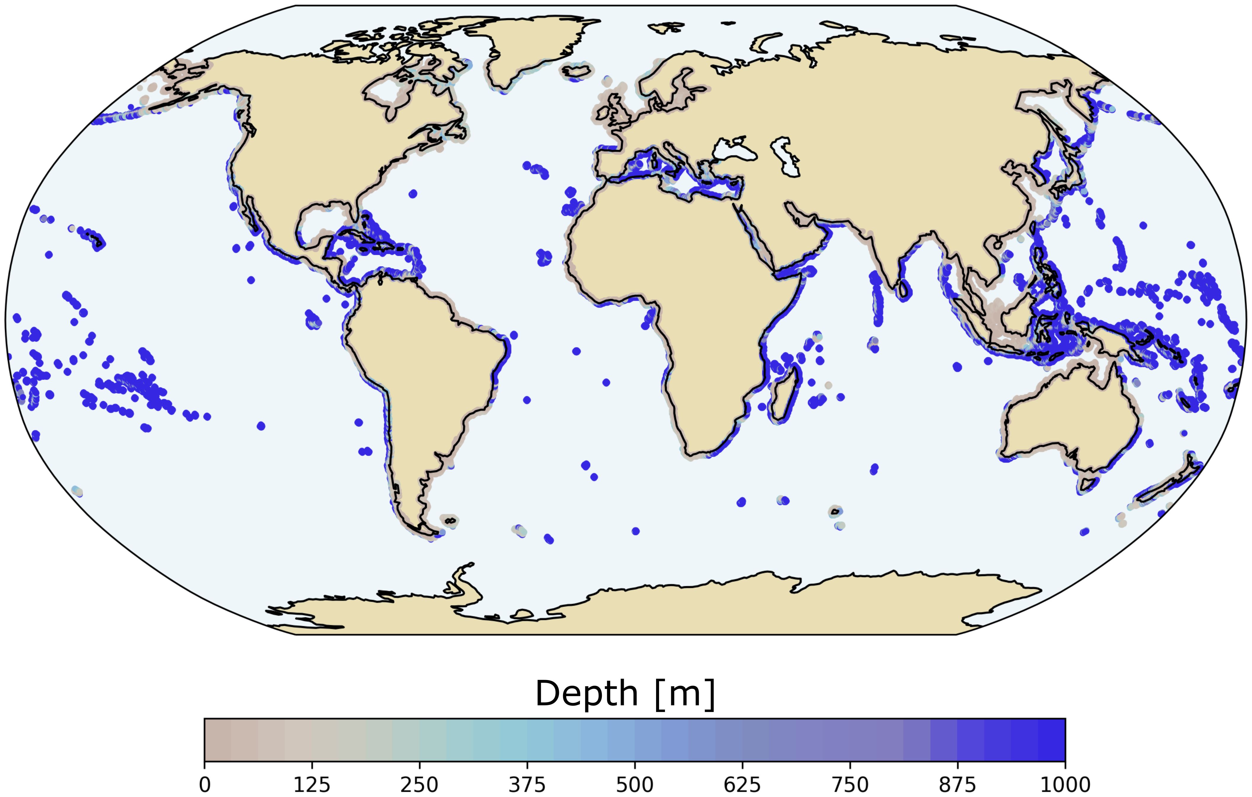
Figure 1 Available directional spectrum data from the wave hindcast.

Recently, the directional wave spectrum from the GOW2 hindcast was fully validated against more than 30 directional wave buoys worldwide (Mazzaretto et al., 2022). The study of Mazzaretto et al. (2022) introduced a methodology for comparing the directional wave spectrum of a hindcast against the one obtained from buoys. This method involves four different approaches and based on several statistical metrics. The initial approach is the global comparison, which compares the time-averaged directional frequency spectrum, frequency spectrum [E(f)] and direction spectrum [E(θ)]. The subsequent approach is the matrix comparison, evaluating the directional wave spectra over time. The third approach is the polar comparison, which examines the frequency-direction bins of the spectrum. Lastly, the 1D spectrum approach compares the E(f) and E(θ) of the hindcast with those from the buoy data. The hindcast directional wave spectrum demonstrates a significant agreement with the buoy data. In the case of the matrix approach (for monthly comparisons), the Pearson correlation coefficient is notably high, exceeding 0.8, and the nRMSE (normalized root mean square error) remains below 9%. The polar approach indicates minimal errors in the hindcast, with directional dispersion matching that of the buoy data. The Pearson correlation coefficient and scatter index metrics show that the higher the energy the higher the agreement, yielding positive outcomes of the wave spectrum validation of the used dataset in this study.

2.2 Wind sea, swell and wave systems estimation method

In order to analyze the climatological conditions of the wave spectra, the wind sea, swells and associated wave systems are estimated. In the present study, a wave system is defined as the long-term conditions prevailing over a frequency-direction wave energy area of the spectrum collecting similar environmental and physical characteristics [following Portilla-Yandún et al. (2015)].

The proposed methodology to characterize the wind sea, swell and associated wave systems (WSys) consists of three steps (Figure 2). This method is applied to each hourly directional wave spectrum (from 1989 to 2020) and for each location (∼ 10.000). The first step (spectrum analysis) computes the hourly sea state spectral partitions, a wind sea, five swells and the residual. This is followed by the second step (partition analysis), which uses the swell partitions to compute the number of occurrences in the frequency-directional domain, namely finding the partitions probability (P_prob). Our P_prob slightly differs from the one proposed by Portilla-Yandún et al. (2015) because we consider only the swell partitions. Furthermore, we apply a filter based on the total m0 of the spectrum at each partition for every time step. Finally, in the third step (wave systems), the long-term swell wave systems are obtained, applying anew the watershed algorithm.

Figure 2

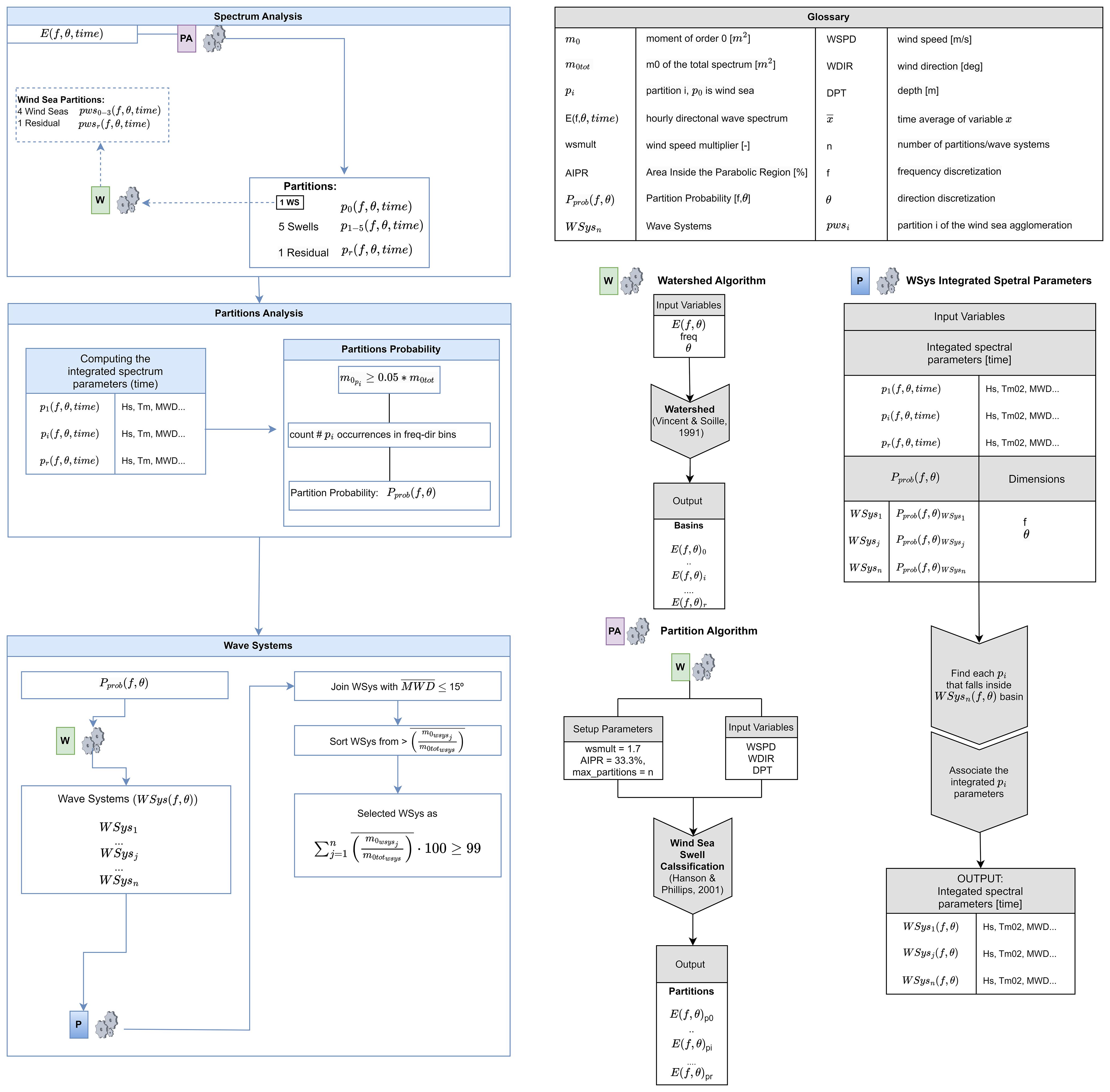
Figure 2 Flowchart of the methodology to find the Swell Wave Systems (WSys) (on the left in light blue), whereas on the right in grey are illustrated the glossary and under it the used algorithms.

The spectrum analysis step initiates processing the directional wave spectrum $(E(f,\theta ,time)[m^2·s/rad])$ of each site at each time through the partition algorithm (, Figure 2). The watershed algorithm (, Figure 2) is first applied, which takes the directional wave spectrum $(E(f,\theta )[m^2·s/rad])$, frequency discretization (f[Hz]) and directional discretization (θ[°]) as inputs and applies the watershed process (, Figure 2), resulting in the extraction of spectral partitions.

Initially, the watershed algorithm was introduced by Vincent and Soille (1991) within the domain of topography for delineating hydrological catchments. Recognizing the analogous nature between the directional wave spectrum and a topographic image enabled the adaptation of the algorithm from topography to the study of oceanic phenomena. This algorithm has undergone further refinement by several researchers and has been implemented in the WWIII model (Hanson and Jensen, 2004; Hanson et al., 2006; Tracy et al., 2007; Tolman et al., 2009).

Once these partitions are obtained, the partition algorithm follows with the classification of the found partitions into wind sea or swells using the approach proposed by Hanson and Phillips (2001). In order to do this, the partition algorithm () receives as inputs the wind speed (WSPD [m/s]), wind direction (WDIR [deg]) and water depth (DPT [m]). Additionally, this algorithm accommodates the inclusion of setup parameters, such as the wind speed multiplier (wsmult[−]), Area Inside the Parabolic Region (AIPR [%]) and the maximum number of partitions that are wanted as output (max partitions [-]). The method proposed by Hanson and Phillips (2001) defines that a partition that lies within the parabolic boundaries,

defined by Equation 1, with at least 33.3% of the area (AIPR) is considered to be forced by the wind and defined as wind sea.

$\begin{array}{ll}{c}_p\le wsmult·U_{10}cos\delta & (1)\end{array}$

where c_p is the phase speed of the partition, U₁₀ is the 10-m elevation wind speed, wsmult is a multiplier of the wind speed and δ is the angle between the wind and the partition. Hanson and Phillips (2001) used wsmult equal to 1.5, to ensure that all possible wind sea peaks are included, whereas we use 1.7 as default in WWIII (Tolman, 2014).

This relationship can be rewritten in terms of the peak frequency: $f_p=\frac{g}{2\pi }{(wsmult·U_{10}\cos \delta )}^{-1}$ with $0\le \delta \le \frac{\pi }{2}$ as in Figure 3.

Figure 3

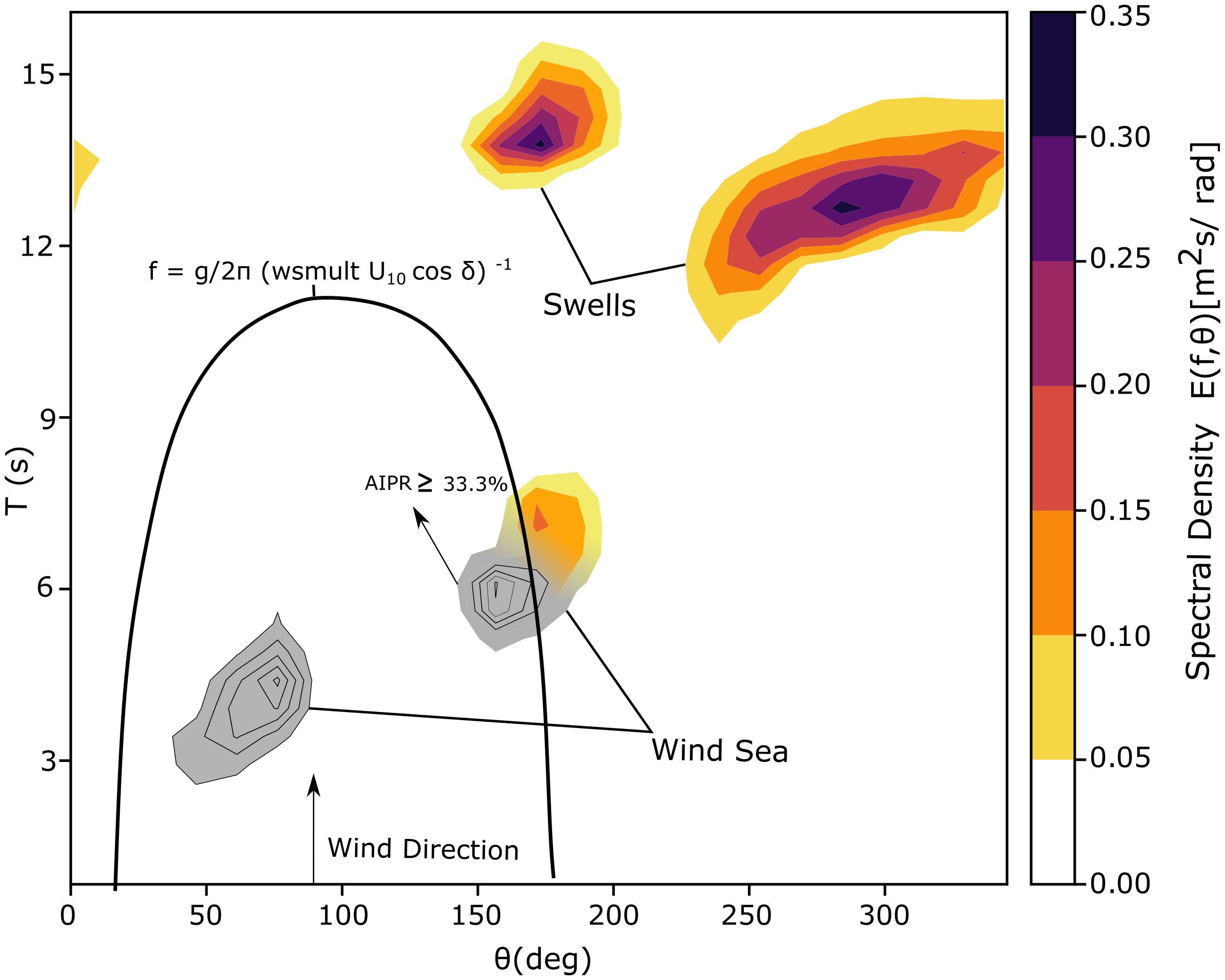
Figure 3 Separation of the wind sea and swell from a directional wave spectrum. Black line shows the parabolic boundary, with 2 wind sea clusters inside.

We note that more than one spectral partition may be inside the parabolic area (Figure 3). All the wind sea partitions from a given input spectrum are combined, the partitions that did not fall in the classification of wind sea are classified as swell and sorted by their significant wave height (H_s).

The default settings for the setup parameters are as follows: AIPR = 33.3%, wsmult = 1.7 and the max partitions is set to six, returning five swells (SWs), $p_{1-5}(f,\theta ,time)$, one wind sea (WS), $p_0(f,\theta ,time)$, and a residual partition, $p_r(f,\theta ,time)$. The latter is the combination of all the partitions that were not combined in the wind sea and that exist after the fifth swell. The consideration of the residual partition is required to avoid energy loss when utilizing the integrated wave parameters of the partitions instead of the total spectrum, particularly in regions characterized by high multimodality when few partitions are obtained e.g. one wind sea and two swells. In addition, the watershed algorithm is applied anew to the aggregation of wind sea partitions, using as input the $p_0(f,\theta ,time)$, storing up to four wind sea partitions $[pw{s}_{0-3}(f,\theta ,time)]$ and one residual, $pw{s}_r(f,\theta ,time)$.

Figure 4 shows the obtained wind sea and swells for an hourly sea state (at 09:00:00 1st of February of 2011) at one of the analyzed locations (lat: 16° N, lon: 17° W). Partition number 0 is the one associated with the wind sea and P1, P2 and P3 are swells. Panel a) of Figure 4 show the hourly sea state wave spectrum and defined partitions in the frequency and directional dimensions. During this event, the wind flew from N (0.38^◦) with a speed of around 9[m/s] (illustrated in Figure 4 as the red arrow). The wind sea is then identified with those partitions whose area falls for more than the 33.3% in the parabolic region defined by Equation 1. Panel b) shows the isolated four partitions from P0 to P3.

Figure 4

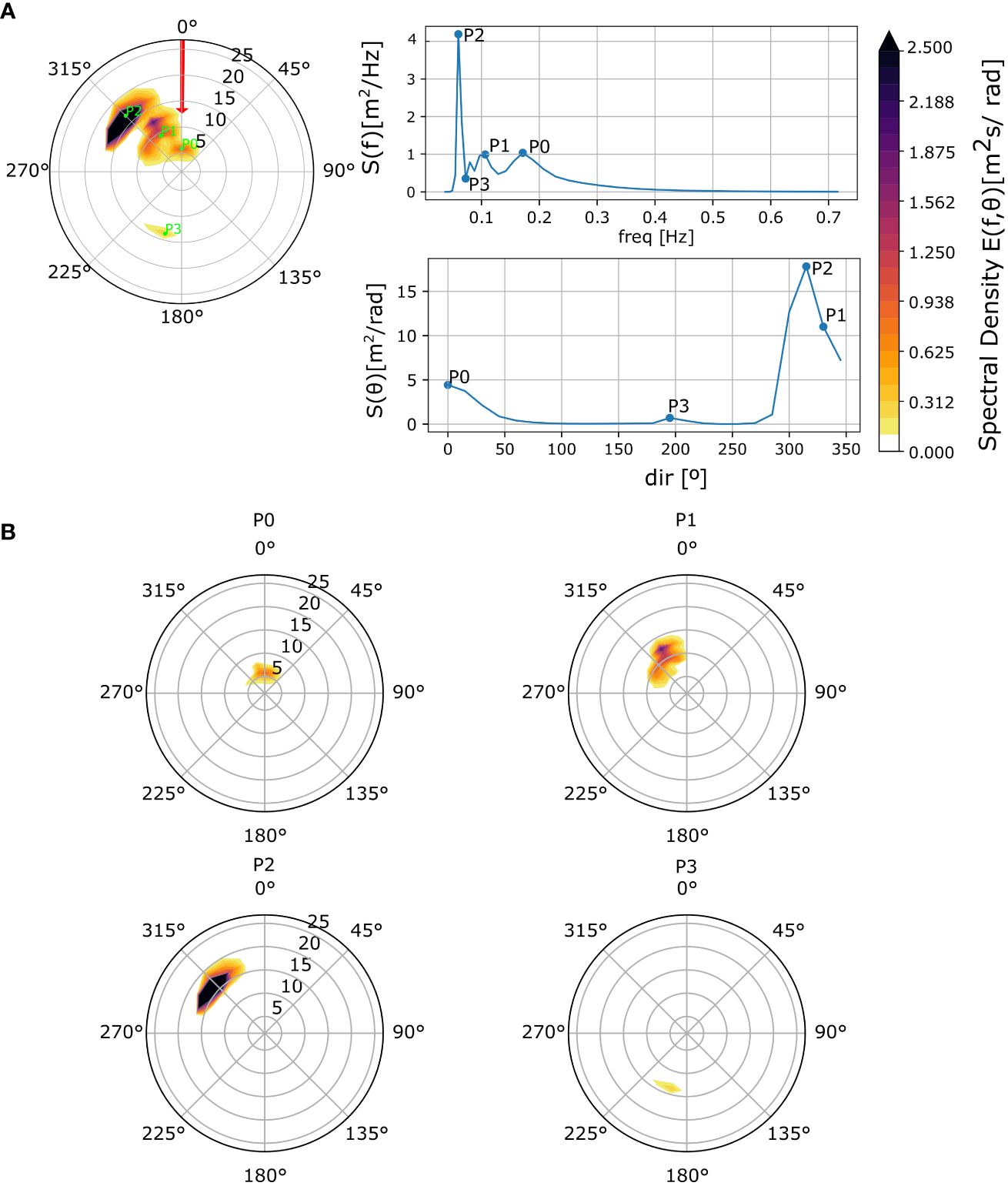
Figure 4 Panel (A) represents the directional wave spectrum for a specific date. The red arrow represents the wind direction. Upper right side of panel (A) shows the associated frequency spectrum and the lower panel shows the direction spectrum. Panel (B) illustrates the partitions of the directional wave spectrum at the selected time. Partition number 0 is the wind sea, while the rest are identified as swells.

Once the spectral partitions are defined, we can proceed with the second step (Partition Analysis). This step starts with the estimation of the integrated spectral parameters such as the significant wave height (H_s), peak period (T_p), mean wave direction (MWD), mean period (T_m02) and peak direction (D_p). They are computed for all the previously identified partitions (i.e. wind sea (WS), five swells (SWs) and the residual).

For this process, only the swell partitions and the residual are considered. We evaluate the energy of each swell partition at each hourly time and identify the swell partitions that have a contribution of at least five percent of the total m₀:

$\begin{array}{ll}{m}_{0_{pi}}\ge 0.05·m_{0_{tot}}& (2)\end{array}$

where $m_{0_{pi}}$ is the moment of order zero of the i-partition (with i going from 1 to r, where r is the residual partition) and $m_{0_{tot}}$ is the total m₀. This condition removes negligible peaks, including the reflection parametrized in the model of WWIII. From the identified T_m02 and MWD of each swell partition, the number of occurrences of 1/T_m02 and MWD in each frequency-direction bin is counted. This led to a new distribution in the frequency-direction space, which we call the Partition Probability (herein after P_prob) $(P_{prob}(f,\theta )[\#Nevents/rad])$ (Figure 5B). The P_prob represents the probability that a certain swell spectral partition of an hourly sea state will fall in a specific frequency-direction bin, therefore each bin encompasses the number of times a partition has belonged to that bin.

Figure 5

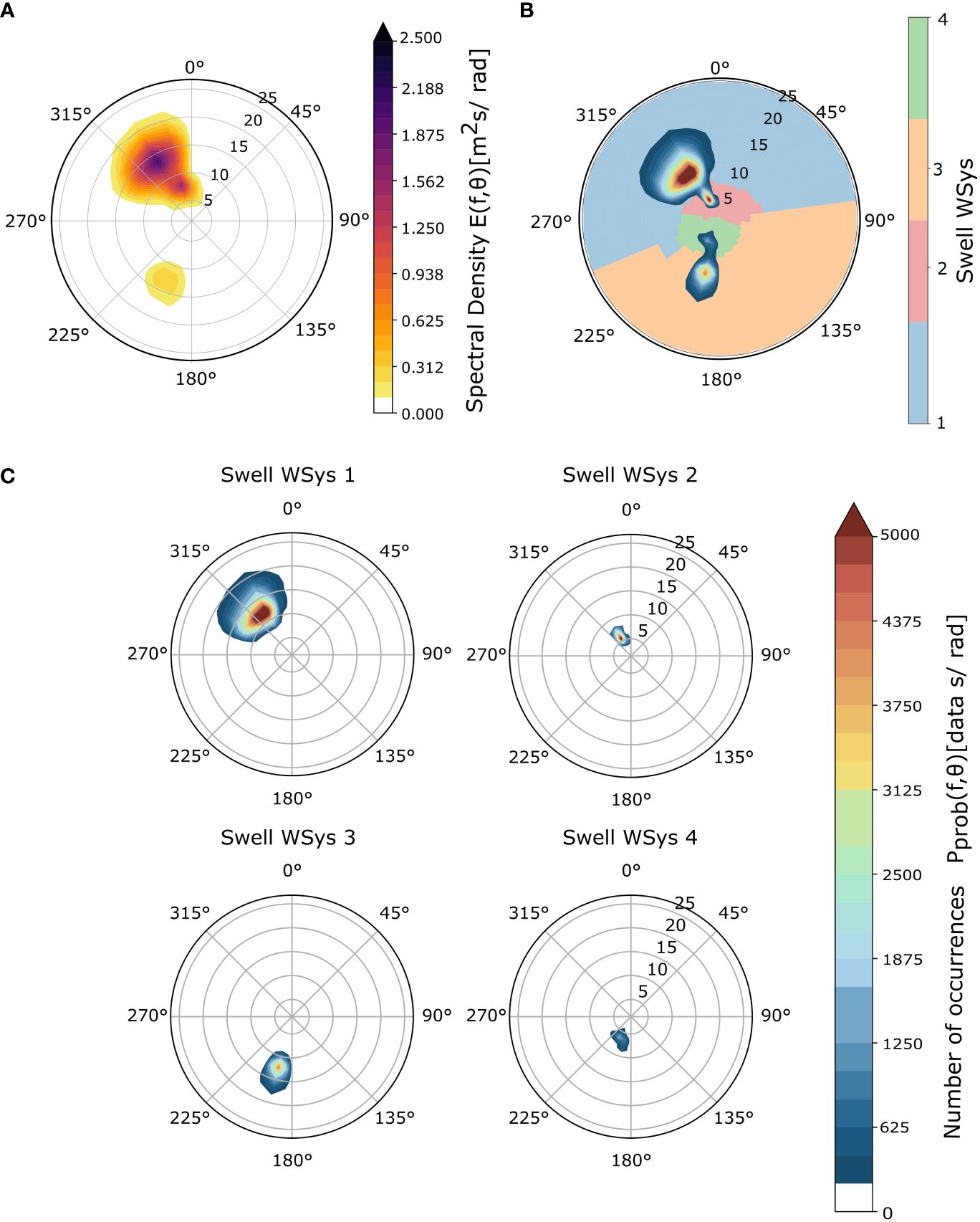
Figure 5 The panels of this figure are referred to the same location in Figure 4. Panel (A) illustrated the time averaged directional wave spectrum. Panel (B) depicts the Partitions Probability and the resulting four swell wave systems. Panel (C) shows each of the obtained swell wave systems.

Finally, the third step identifies the swell wave systems. As in Portilla-Yandún et al. (2015); Portilla-Yandún (2018) we apply a clustering algorithm (the watershed algorithm is applied anew) to the $P_{prob}(f,\theta )$, using the same frequency f [Hz] and directional discretization θ [°] of the directional wave spectrum. From this process the swell wave systems are obtained and up to eleven swell wave systems $(WSy{s}_1,\dots ,WSy{s}_j,\dots WSy{s}_n)$ are stored. Successively, the third step follows with the swell wave system integrated spectral parameters algorithm (), which receives as input the integrated spectral parameters of each swell partition (p₁−_r), the $P_{prob}(f,\theta )$ of each swell wave systems $WSy{s}_{1-n}(f,\theta )$, the same frequency [f(Hz)] and directional discretization θ [°] of the directional wave spectrum. The swell partitions that fall in each swell $WSy{s}_j(f,\theta )$ are found, and the integrated spectral parameters of these partitions are associated to obtain the time series parameters corresponding to each swell wave system.

Figure 5 depicts the 32 year time averaged directional wave spectrum (panel A). The values of P_prob (number of occurrences) are shown in Figure 5B, for the total P_prob. In Figure 5C, the found four swell wave systems are depicted. The colorbar on panel a) represents the energy corresponding to the directional wave spectrum, whereas the colorbar in Figure 5B shows the watershed output, which defined the swell wave systems. The colorbar in Figure 5C depicts the number of spectral partitions of an hourly sea state that fall in a specific frequency-direction bin.

Some locations (Figure 6), such as the indicated in the West Japanese coast [36.50°N; 141.25°E] have a wide directional distributed time-averaged spectrum, with higher energy focused between 40° and 90°. The rest of the energy comes from 225° to 90°, but with less intensity. Conversely, the P_prob, on the right side, depicts three clearly defined WSys, one coming from 42°, another from 100° and the last from 180°. Central panel in Figure 6, illustrates the mean wave spectrum for a location in northern Spain [43.75°N;3.75°W]. The mean wave spectrum (on the left) shows only one clear section, where the waves come from the NW, however, the sea states from NNE direction associated with low energy are hidden. P_prob on the right shows that these events, although not so energetic, can be frequent. The last case depicted in Figure 6 illustrates a coastal location in the Gulf of Mexico [17.00°N;101.25°W]. From the left panel, only two well-defined partitions are identified, however, in the left panel, a swell wave system with a high probability to occur but with low energy is clearly distinguishable and six swell wave systems are encountered.

Figure 6

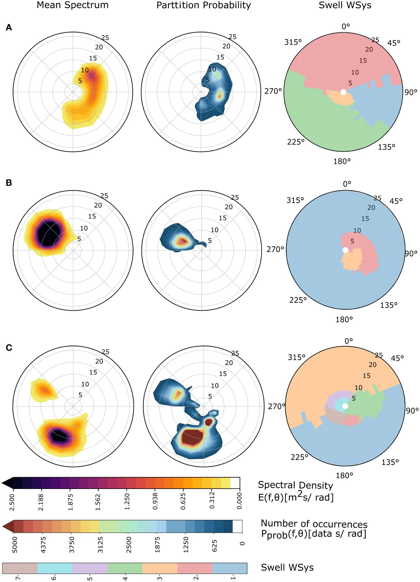
Figure 6 The first column represents the time averaged directional wave spectrum. Second column represents the Partition Probability and the last column is the watershed of the Partition Probability. The rows illustrate three different regions worldwide, first row (A) represents a node in western Japan, the second (B) is a location in northern Spain and the last one, (C), is a location in the Mexican Gulf.

After obtaining the P_prob of the swell wave systems, for each swell wave system, the time series of the integrated spectral parameters are computed. Successively, the swell wave systems with less than 15°

difference on the time averaged MWD are joined. Finally, the swell wave systems are sorted for their time averaged supply of m0 to the total $(m_{0_{SwellWSy{s}_j}}/m_{0to{t}_{SwellWSys}})$ and the number of significant swell wave systems is obtained when the sum of the ratio of the m₀ of the i-WSys, and $m_{0to{t}_{SwellWSys}}$ averaged in time reached at least 99%:

$\begin{array}{ll}\frac{1}{N_t}{\displaystyle \sum _{i=1}^N}\left[{\displaystyle \sum _{it=1}^{N_t}}{\left(\frac{m_{0_i}}{m_{0to{t}_p}}\right)}_{it}\right]·100\ge 99& (3)\end{array}$

where $m_{0_i}$ is the m₀ of the i-WSys, N is NWSys (the number of swell wave systems, in this case, eleven), N_t is the number of sea states and $m_{0to{t}_p}$ is $m_{0to{t}_{SwellWSys}}$ the order zero momentum for the total swell wave systems.

3 Results

3.1 Wind sea and swell climate conditions

The characterization of wind sea and swell is crucial for a wide variety of research and engineering studies such as analyzing the movement of a mooring ship. The oscillations experienced by the mooring ship within bimodal spectral waves exhibit considerably greater magnitudes compared to those observed for only wind sea (Shi, 2018). In contrast, the pure wind sea in floating wind turbines can contribute to low-frequency resonant oscillations (Chakrabarti, 2005; Brommundt et al., 2012). Therefore, the energy and time dominance of the wind sea and swells is analyzed.

The time dominance is defined as shown in Equation 4.

$\begin{array}{ll}\begin{array}{l}\frac{1}{N_t}{\displaystyle \sum _{it=1}^{N_{\text{t}}}}(m_{0_{\text{WS},it}}>m_{0_{\text{tot}}}·0.75)·100\to \text{\% of time the dominant is WS}\\ \frac{1}{N_t}{\displaystyle \sum _{it=1}^{N_{\text{t}}}}({\displaystyle \sum _{isw=1}^{N_{\text{SWs}}}}{m}_{0_{\text{isw},\text{ it}}}>m_{0_{\text{tot}}}·0.75)·100\to \text{\% of time the dominant is SWs}\\ \frac{1}{N_t}{\displaystyle \sum _{it=1}^{N_{\text{t}}}}(m_{0_{\text{tot}}}·0.25\le m_{0_{\text{WS},it}}\le m_{0_{\text{tot}}}·0.75)·100\to \text{\% of time WS and SWs have similar energy}\end{array}& (4)\end{array}$

where $m_{0_{WS}}$ is the zeroth order momentum of the wind sea, $m_{0_{tot}}$ is the zeroth order momentum of the total spectrum, $m_{0_{SWs}}$ in the zeroth order momentum of the swells. We identify the percentage of time in which the wind sea persists with Equation 4, namely, it is the percentage of the time in which the wind sea has more than 75% of the total energy. Similarly, the swells and, when the $m_{0_{WS}}$ is in the interquartile range of the $m_{0tot}$, then we consider that the swells and the wind sea coexist.

Figure 7 shows the percentage of time in which the SWs or the WS persists from the hourly data analyzed during the 32yrs historical period. The upper panel (Figure 7) shows the swell partitions, whereas, the lower panel (Figure 7) depicts the wind sea. In Figure 7 can be seen that, overall, on the West coast of the continents, the swells persist during the considered time, while on the East coast and for enclosed Seas the wind sea persists longer than the swells. On the coasts of Indonesia facing the ocean the SWs persist more than the WS, whereas, in the small enclosed region between all these islands, the wind sea and swells persist together. In the southern part of Cambodia and Vietnam, the wind sea persists more than the swells. The persistence of the wind sea is also high in the Baltic Sea, whereas in the Mediterranean Sea, the persistence of the WS is not absolute due to the fact that in this region, swells also persist during the analyzed time.

Figure 7

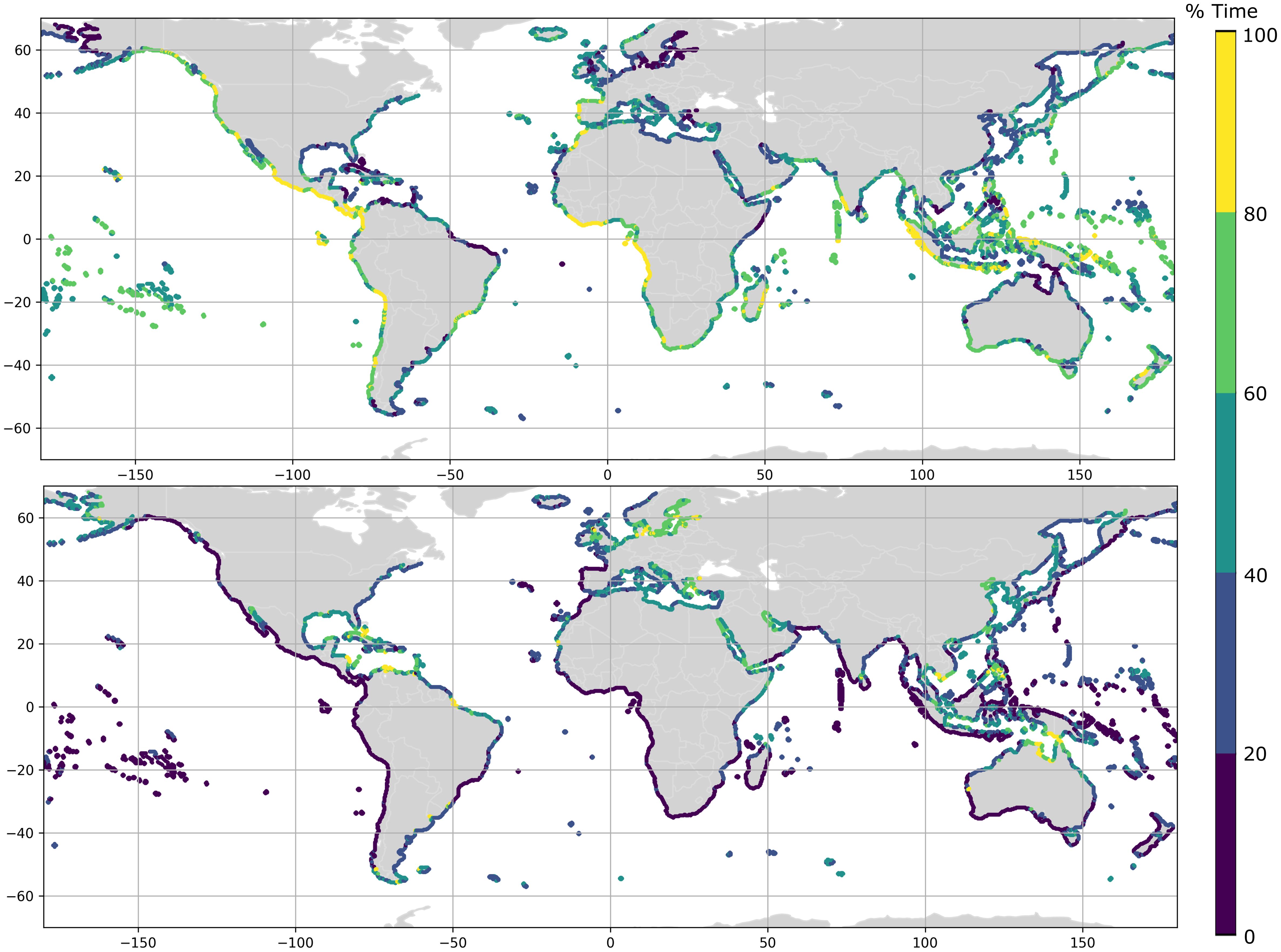
Figure 7 Persistence in time. Percentage of the WS (bottom) and the SWs (top).

Instead of a time analysis, an energy analysis is also carried out. The energy dominance is then carried out using Equation 5.

$\begin{array}{ll}\begin{array}{l}\frac{1}{N_t}{\displaystyle \sum _{it=1}^{N_t}}{\left(\frac{m_{0_{WS}}}{m_{0_{tot}}}\right)}_{it}>0.75\to \text{wind\hspace{0.17em}sea\hspace{0.17em}dominant}\\ \frac{1}{N_t}{\displaystyle \sum _{it=1}^{N_t}}{\left(\frac{{\sum }_{isw=1}^{N_{SWs}}{m}_{0_{isw}}}{m_{0_{tot}}}\right)}_{it}>0.75\to \text{swells\hspace{0.17em}dominant}\\ 0.25\le \frac{1}{N_t}{\displaystyle \sum _{it=1}^{N_t}}{\left(\frac{m_{0_{WS}}}{m_{0_{tot}}}\right)}_{it}\le 0.75\to \text{mixed\hspace{0.17em}conditions}\end{array}& (5)\end{array}$

where $m_{0_{WS}}$ is the m₀ of the wind sea partition, $m_{0_{tot}}$ is the m₀ of the total spectrum, and the ${\displaystyle {\sum }_{isw}^{Nswells}{m}_{0_{isw}}}$ represents the sum of the m₀ of each swell partition. WS is dominant when the ratio of its moment 0 to the total m₀ averaged over time (3h resolution, for the 32 years) is greater than 75%. Conversely, when the ratio of the sum of the swell moment 0 to the total m₀ is greater than 75%. Finally, the partitions coexist when the ratio of the m₀ of the wind sea to the $m_{0_{tot}}$ is between 25% and 75%.

The results are shown in Figure 8, which illustrates the worldwide distribution of dominant partitions on the coast. We note that the swells coexist with the wind sea almost 70% of the analyzed nodes, whereas 25% of the global coast is dominated by the swells (typically the westers coasts). Only the 5% is dominated by the wind sea (such as the Gulf of Carpentaria, the Baltic Sea, and the Aegean Sea).

Figure 8

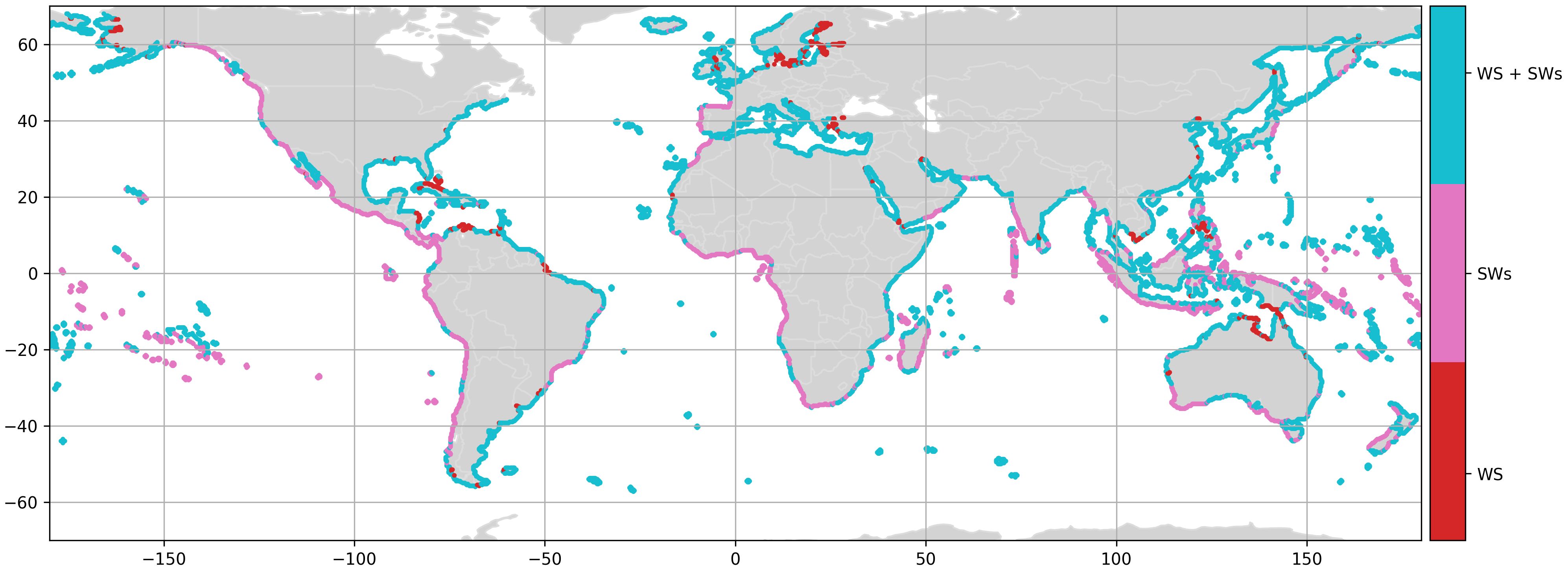
Figure 8 Red color identifies the dominance of the wind sea (WS), pink color shows the dominance of the swell (SW) and blue coor indicates the usual coexistence of wind sea and swell.

The localized regions in which the WS or the swells dominated in energy also persist longer on time. We note that the areas in which the dominance belongs to the coexistence of WS and SWs does not mean that the persistence in time has to be distributed equally to the WS and the swells. For the dominance, we consider the time-averaged 0th order moment higher than the 75% of the $m_{0tot}$, nonetheless, for the persistence in time, we consider the percentage of the time in which one partition is higher than the 75% of the $m_{0tot}$.

A thorough seasonal analysis is conducted to uncover prevailing patterns of wind seas and swells across various geographical regions. Generally, regions where swells dominate exhibit relatively fewer variations due to seasonal transitions. However, noteworthy alterations become apparent during specific timeframes. For instance, along the coast of Ecuador during June, July, and August (JJA) a shift from predominant swell dominance to a coexistence of wind seas and swells is noticed. Similarly, during March, April, and May (MAM), significant changes are observed along the Pacific coast of Baja California, where swells relinquish their dominance to accommodate a coexistence of wind seas and swells. Throughout December, January, and February (DJF), the Baltic Sea, the Horn of Africa, and the northern coast of Cuba, previously characterized by a mixed coexistence of wind seas and swells (Figure 8), shift primarily towards wind sea dominance. This trend also holds true for the Sea of Okhotsk, with the exception of other seasons when wind seas and swells coexist dominantly. Conversely, the Gulf of Carpentaria remains consistently dominated by wind seas across all seasons. Prominent deviations from average values (Figure 8) are evident during JJA season. Along the Atlantic coast of Morocco, the Maranhão and Cerá regions of Brazil, and the Horn of Africa the wind sea dominates. In contrast, the Baltic Sea experiences an inverse trend, with the coexistence of swells and wind seas. During September, October, and November (SON), significant shifts occur in the Maranhão and Cerá regions of Brazil, where the wind sea dominance is prevalent. Meanwhile, swells primarily dominate in the Micronesia islands during this period.

In addition to the aforementioned study, we also examine the aggregation of wind seas. We estimate the wind sea partitions as illustrated in Figure 2, once the directional wave spectrum is processed through the partition algorithm, one wind sea, five swells and one residual partitions are obtained. The methodology of Hanson and Phillips (2001) agglomerates the partitions that fall inside the parabolic region with more than 33.3% of the AIPR as one wind sea. We have applied the clustering algorithm to the agglomeration of wind seas and stored up to four wind seas and a residual partition. Figure 9 precisely illustrates the number of independent wind seas. We defined the number of independent wind seas as the number of wind sea partitions that account for at least 99% of the total zeroth momentum of the wind seas $(m_{0to{t}_{WS}})$ using Equation 3. Where $m_{0_i}$ is the $m_{0_{W{S}_i}}$ of the i-WS, N is NWS (the number of wind seas, in this case, five) and $m_{0to{t}_p}$ is $m_{0to{t}_{WS}}$ (order zero momentum for the total wind seas).

Figure 9

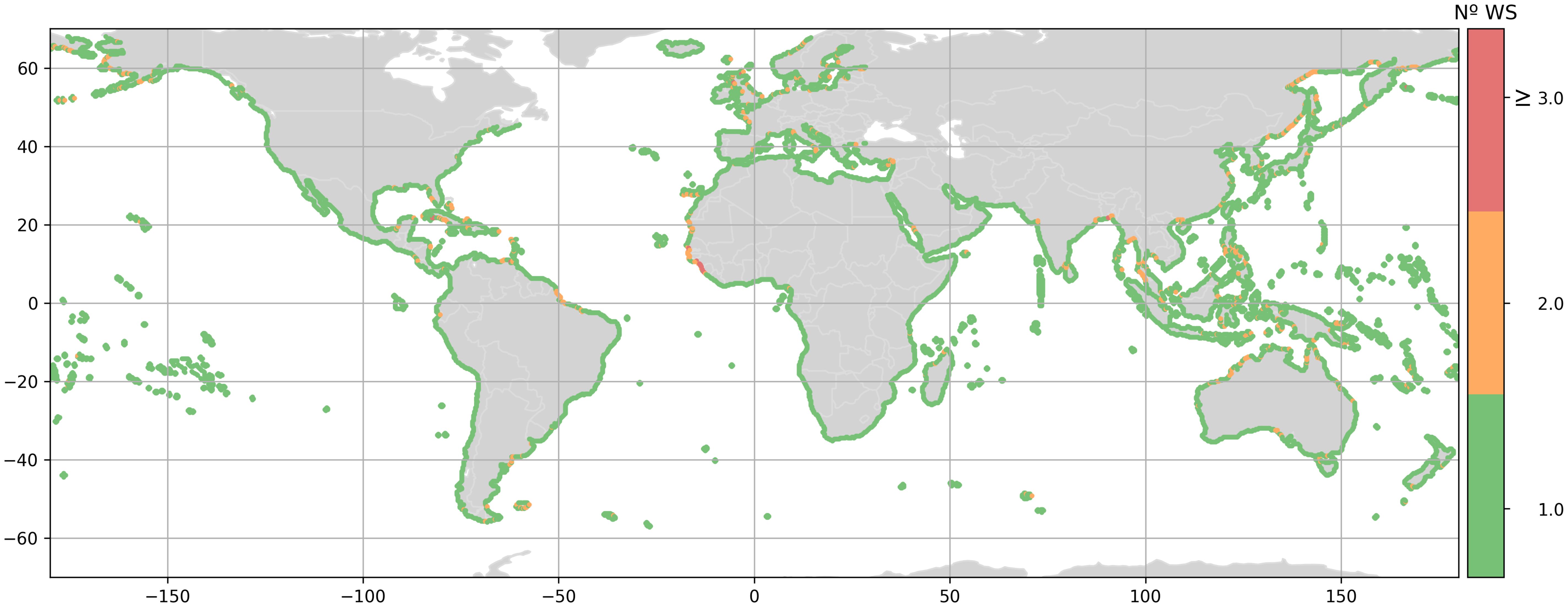
Figure 9 Number of identified wind seas (WS).

The analysis reveals that approximately 93% of the global coastline is predominantly dominated by a single wind sea partition. Only 7% of the world exhibits the presence of two or more wind sea partitions agglomerations. Two wind seas are primarily observed in semi/enclosed seas and coastlines over regional gulfs such as the Adriatic Sea, South Tyrrhenian Sea, Libyan Coast, Baltic Sea, Northern Sea, Gulf of Carpentaria, Japanese Sea, Okhotsk Sea, and the West coast of Florida. The only region that shows more than three wind seas is concentrated along the coast from Southern Senegal to Sierra Leone.

3.2 Swell wave systems

The swell wave systems provide long-term information of the frequency-direction wave energy distribution. These swell wave systems group together all the swell spectral partitions of each historical hourly sea state with similar characteristics. Thus, each swell wave system is described by a wave period and mean wave direction. In addition, the percentage of energy it represents with respect to the total spectrum can be estimated. This information is especially useful to identify those secondary swells, which can impact the coast and are usually masked by the dominant swell. The number of found significant swell wave systems, calculated using Equation 3, along the coast worldwide is displayed in the Figure 10.

Figure 10

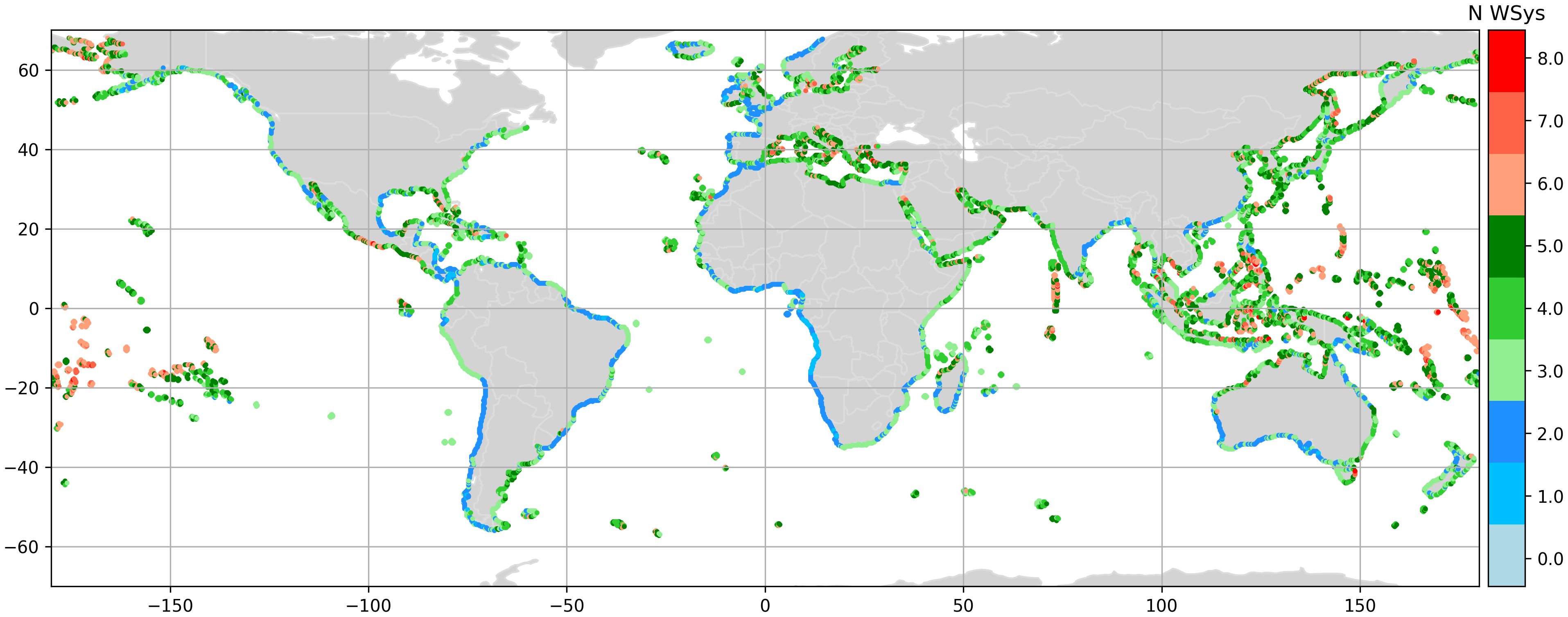
Figure 10 Number of significant swell wave systems.

It is noteworthy that the majority of regions exhibit the dominance of three or four swell wave systems, accounting for 26% and 25% respectively. A 15% of the analyzed coastal locations show two swell wave systems. The wave climate conditions characterized by a single swell wave system appears only on the 2% of the world’s coastline. The presence of five swell wave systems is found for the 19% of the global coast, whilst a mere 13% of the analyzed locations have six or more swell wave systems.

In the Gulf of Angola, the dominant partitions are swells (Figure 8) clustered in one significant swell wave system. Other regions such as the Atlantic Coast of Ireland, South and West coast of Australia, Atlantic coast of Spain, Portugal, Morocco and the coast of Chile are dominated by two swell wave systems. Nonetheless, it is easy to find regions with three or four swell wave systems, such as the coast of Japan, South Africa, North and East coast of Australia. North America is dominated by two swell wave systems up to five. The regions with most swell wave systems are in correspondence to the Mexican pacific area. Asia, the Mediterranean Sea, the Baltic Sea and the Red Sea are principally dominated by four to five swell wave systems. Most of the islands corresponding to Oceania have at least four or above swell wave systems.

The wave systems can be visualized by their mean values of peak period, mean wave direction and the m₀. Figure 11 depicts an example of the results for a single analyzed location, offshore of Santander, northern Spain (lat: 43.75, lon: -3.75). It shows three arrows, corresponding to two swell wave systems and the wind sea. The size of the arrows is associated to the mean peak period, the mean wave direction is represented by the direction of the arrow and the color is the percentage of m₀ respect the total $m_{0_{tot}}$. This location is characterized by a primary swell wave system (NW), a wind sea (NNW) and a secondary swell wave system (NE). The primary swell wave system possesses the 71.1% of the total m₀, the wind sea the 22.2% and the secondary swell wave system the 6.3% of the $m_{0_{tot}}$. The primary swell wave system represents the 92% of the total swell energy, and the secondary swell wave system the 8%. Analyzing the historical time occurrence, we find that the primary swell wave system (NW) is very usual, happening during the 88% of the historical period. The secondary swell wave system has however a higher occurrence through time than percentage of total energy (18% of the time for all the historical period). The NE wave system has also lower peak period and it is more apparent during the summer season.

Figure 11

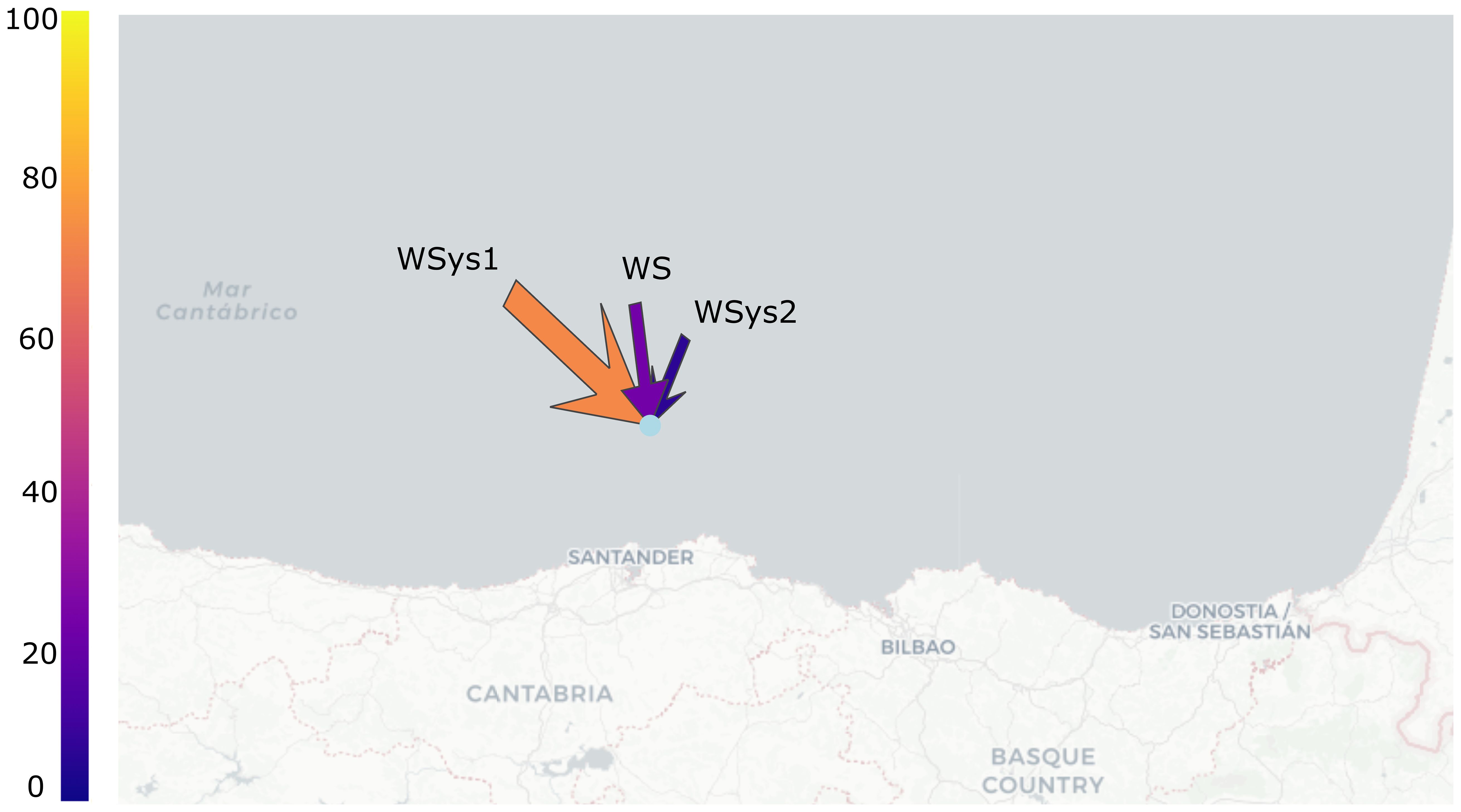
Figure 11 Graphical illustration of the wave systems for a single location, situated offshore of Santander, northern Spain (lat: 43.75, lon: -3.75). WSys1 corresponds to the primary swell wave system, WS is the wind sea and WSys2 is the secondary swell wave system. The size of the arrow is the mean wave period, the direction is the mean wave direction and the color represent the percentage of energy for each wave system.

Figure 12A provides a close-up view of the Iberian peninsula in the Strait of Gibraltar. The Atlantic coast is primarily dominated by a western swell wave system. As we move further into the Mediterranean Sea, we observe the convergence of swell wave systems originating from both the Mediterranean and the Atlantic, resulting in the presence of at least two swell wave systems with similar $m_{0_{SwellWSys}}$, one from the east and another from the west. The swell wave system originating from the Mediterranean Sea exhibits a shorter period compared to the Atlantic swell wave system, as indicated by the size of the arrows.

Figure 12

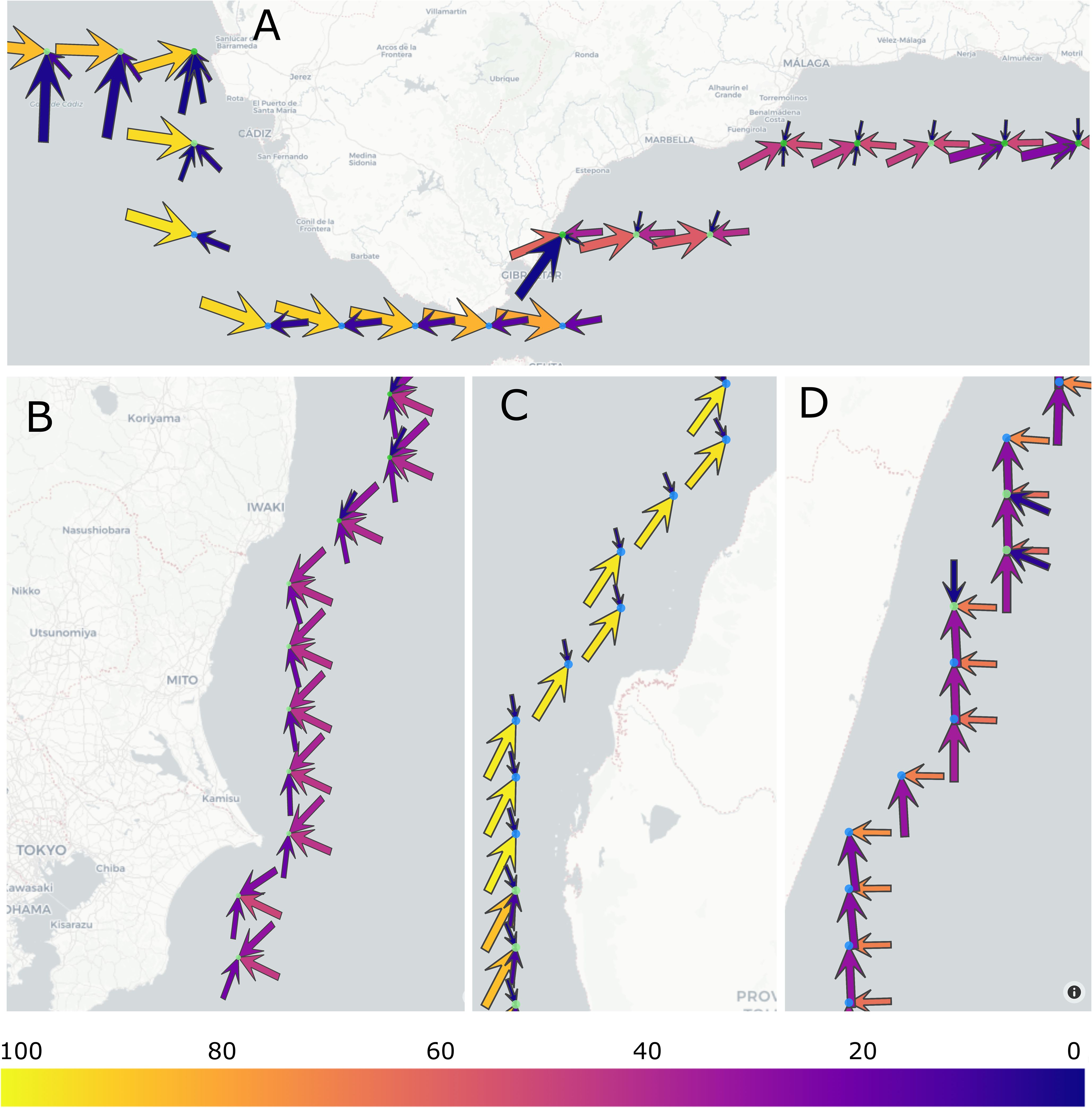
Figure 12 Detected swell wave systems along coastal areas. The color identifies the relative energy of each swell wave system as the percentage with respect to the total swell energy. The size of the arrow represents the mean Tp. The number of the arrows are the identified swell wave systems for each location. The direction of the arrow represent the MWD where the swell wave systems come from. Panel (A) shows the strait of Gibraltar, panel (B) the East coast of Japan, near Tokyo and panels (C) and (D) show the West and East coast of Madagascar island (between 18-22°S).

Figure 12B depicts the West coast of Japan near Tokyo. In this region can be appreciated three significant swell wave systems, two of them providing about 40% of $m_{0_{SwellWSy{s}_i}}/m_{0to{t}_{SwellWSys}}$ each and about the 20% for the third swell wave system. The primary swell wave system come from ESE, the second from NE and the third from S, their peak periods are similar and around 9 seconds.

Figures 12C, D illustrate the West and East coast of Madagascar island between 18-22^◦S, in this region, for both sides of the island, the swell coming from the Southern Ocean is present, albeit with different percentage of $m_{0_{SwellWSys}}$. This disparity arises from the exposure of the East coast of Madagascar to swells generated in the Indian Ocean, which arrive eastern onto the island. Consequently, the eastern swell wave system possesses 73% of the $m_{0to{t}_{SwellWSys}}$, while the southern component accounts for the remaining 26%. As we move forward to the West coast of Madagascar the restricted fetch inhibits the generation of significant swell wave systems, resulting in the predominance of the swell wave system originating from the SSW, which constitutes 97% of the $m_{0to{t}_{SwellWSys}}$.

Another interesting region of study is North America, starting from Baja California, where two significant swell wave systems are observed, one from the south and the other from the north. As we move northwards, we observe a notable transition as the energetically dominant swell wave system from the south gradually

gives way to the swell wave system originating from the north. This transition is particularly evident near the coast of Los Angeles, where the change appears to be more pronounced. Further north, the swell wave system from the north becomes a westward-propagating swell wave system, indicating that from this point on, the northern storms directly impact the American coasts of Oregon and Washington. Despite this transition, remnants of the southern Pacific swell wave system is still appreciated in these regions.

The global outcomes of this analysis can be explored through a web viewer (https://ihcantabria.github.io/WaveSystemsViewer/). This web viewer initially presents the count of significant swell

wave systems. Upon selecting one of the nine regions (Africa, Europe, North America, South America, Asia 1 to Asia 3, and Oceania 1 to 2), and zooming in a coastal area, additional layers of detail are revealed. The swell wave systems are visually represented through a quiver plot. The number of arrows corresponds to the count of significant swell wave systems, and each color of the arrow signifies the relative energy proportion of the respective swell wave systems. This energy ratio is expressed as a percentage:

$m_{0_{SwellWSy{s}_i}}/m_{0to{t}_{SwellWSys}}$. The arrow size conveys the time-averaged T_p, while the quantity of arrows denotes the prevalence of swell wave systems in a given location. The direction of each arrow indicates the time-averaged MWD from which the swell wave systems come. Further information is available in the Supplementary Material.

4 Conclusions

Partitioning a directional wave spectrum allows for the identification and classification of specific wave components such as wind sea or swell. This classification process facilitates a comprehensive analysis of the global wave climate, encompassing more than 30 years of 3-hourly data. Regions where either swells or wind sea dominate are identified, providing insights into the prevailing wave characteristics in different areas. The results reveal that swells and wind sea coexist in approximately 70% of the global coast, particularly in enclosed seas and the eastern regions of the continents. Conversely, around 25% of the global coast is primarily dominated by pure swells, with the majority of this percentage located along the western coastlines of the continents. In contrast, a mere 5% of the global coast is dominated by the wind sea, primarily observed in highly enclosed seas such as the Baltic Sea, the Eagan Sea, and the Gulf of Carpentaria. The regions in which the swell dominate over the wind sea match with those in which the swell probability is higher according to Chen et al. (2002). Further investigation should aim to a global time-dependent monthly analysis of the swell wave systems in order to better understand the wave climate variability. For example, Alonso and Solari (2021) conducted a Uruguayan nationwide scale study of the wave systems seasonal and inter annual variations, using a high-resolution wave hindcast. In addition, an extreme analysis that associates storm event to each wave system would be of interest, as it would allow to understand which component is the most energetic during extreme events. Portilla-Yandún and Jácome (2020) use the wave system decomposition to perform extreme value analysis and applied the POT methodology to the wave systems. The same extreme analysis could be carried out seasonally/monthly. It is worth mentioning that every location has different characteristics, and thus requires a specific study.

The climatic persistence of these partitions was also studied. In some regions, such as the Gulf of Angola, the west coast of Mexico, the west coast of Indonesia and the coast of Portugal the swells persist for most of the time. Conversely, in more enclosed areas, such as the Gulf of Carpentaria, the Baltic Sea and Cambodia, the wind sea persists for the majority of the time. Other regions, such as India, Northern Spain and the west coast of South America have a swell between 60-80% of the time.

The definition of the wind sea, proposed by Hanson and Phillips (2001), groups together all the wind seas, therefore it can result in more than one wind sea inside the wind sea partition. Although the wind sea dominates only 5% of the total coast, it coexists for approximately 70% of the coast. Thus it is important to understand how many wind seas are grouped in the wind sea definition. Results have shown that, on average, one significant wind sea exists (93% of the total coast), although there are different regions distributed all around the world in which two wind seas are found. The outstanding region where more than three wind seas are found is situated in Africa (between Southern Senegal and Sierra Leone). In these regions the definition of wind sea proposed by Hanson and Phillips (2001) may be further studied for a better comprehension of the wave climate.

The clustering of the swell wave partitions has facilitated the identification of different wave systems. In this study, we define a wave system as wind sea or a collection of swells that consistently originate from a specific sector within the frequency-direction domain. By computing the probability of the swell partitions that satisfy the criteria outlined in Equation 2, we have then cluster them in order to get new insights about the swell wave climate conditions. Notably, the results indicate that approximately the 51% of the global coast exhibits the prevalence of three and four swell wave systems, while approximately 15% demonstrate a dominance of two swell wave systems. In contrast, a single swell wave system is observed in only 2% of the global regions. Moreover, approximately 32% of the regions studied, primarily small islands in the Pacific Ocean and enclosed seas, have at least five swell wave systems are present. Coastal areas such as the straits, present the behavior of two opposite swell wave systems (for example, Baltic Sea, Red Sea, Strait of Gibraltar and the British Channel), whereas enclosed seas and open ocean islands are characterized by multiple swell wave systems coming from multiple directions. Having a close look to the west coast of the Iberian peninsula it can be seen that the principal swell comes from the north, consistent with the findings of Semedo et al. (2008) and de Farias et al. (2012). The analysis of the swell wave systems allows identifying also those swell wave systems that have less frequency and generally develop at regional scale or coming from another generation area and persisting to the coast. Such behavior can also be observed along the Chilean coast where the primary swell come from South, in agreement with the results of Semedo et al. (2008); de Farias et al. (2012). However, the secondary swell wave system (NW) can only be detected by the proposed the swell wave system analysis. Accordingly with the study of Alonso and Solari (2021), the main swell wave systems along the Uruguayan coast comes from the South and the East. A comparison of the found wave systems with the study from Portilla-Yandún and Jácome (2020) at a location near the Colombian coast, also indicates similar results, with four significant swell wave systems, two coming from the SW quadrant and the other two coming from the NE quadrant.

In conclusion, it is noteworthy that the prevalence of wind sea and swells coexistence characterizes the majority of the global coastline, with only a few areas being dominated by pure swells. The significance of swell wave systems lies in the fact that over half of the global coastline experiences the influence of three to four distinct swell wave systems. Merely 2% of the global coast is impacted by a single swell wave system. Notably, in tropical and equatorial regions, more than five swell wave systems are required to encompass 99% of the total swell wave system energy.

Data availability statement

The outcome values of this study are available through the web viewer. The supplementary material indicates how to obtain the information through the viewer. The raw data analyzed in this study are available under request. Requests to access these datasets should be directed to the email adress: ihdata@ihcantabria.com.

Author contributions

OM: Methodology, Formal analysis, Data curation, Writing – original draft, Writing – review & editing. MM: Conceptualization, Formal analysis, Funding acquisition, Supervision, Writing – original draft, Writing – review & editing.

Funding

The author(s) declare financial support was received for the research, authorship, and/or publication of this article. The authors acknowledge financial support by the ThinkInAzul programme, with funding from European Union NextGenerationEU/PRTR-C17.I1 and the Comunidad de Cantabria.

Conflict of interest

The authors declare that the research was conducted in the absence of any commercial or financial relationships that could be construed as a potential conflict of interest.

The author(s) declared that they were an editorial board member of Frontiers, at the time of submission. This had no impact on the peer review process and the final decision.

Publisher’s note

All claims expressed in this article are solely those of the authors and do not necessarily represent those of their affiliated organizations, or those of the publisher, the editors and the reviewers. Any product that may be evaluated in this article, or claim that may be made by its manufacturer, is not guaranteed or endorsed by the publisher.

Supplementary material

The Supplementary Material for this article can be found online at: https://www.frontiersin.org/articles/10.3389/fmars.2024.1385285/full#supplementary-material

References

Alonso R., Solari S. (2021). Comprehensive wave climate analysis of the Uruguayan coast. Ocean Dynamics 71, 823–850. doi: 10.1007/s10236-021-01469-6

CrossRef Full Text | Google Scholar

Alvarez-Cuesta M., Toimil A., Losada I. (2021a). Modelling long-term shoreline evolution in highly anthropized coastal areas. part 1: model description and validation. Coast. Eng. 169, 103960. doi: 10.1016/j.coastaleng.2021.103960

CrossRef Full Text | Google Scholar

Alvarez-Cuesta M., Toimil A., Losada I. (2021b). Modelling long-term shoreline evolution in highly anthropized coastal areas. part 2: assessing the response to climate change. Coast. Eng. 168, 103961. doi: 10.1016/j.coastaleng.2021.103961

CrossRef Full Text | Google Scholar

Amante C., Eakins B. W. (2009). ETOPO1 arc-minute global relief model: procedures, data sources and analysis. Series: NOAA technical memorandum NESDIS NGDC; 4. Available at: https://repository.library.noaa.gov/view/noaa/1163.

Google Scholar

Ardhuin F., O’reilly W., Herbers T., Jessen P. (2003). Swell transformation across the continental shelf. Part I: Attenuation and directional broadening. J. Phys. Oceanography 33,

Google Scholar

Ardhuin F., Rogers E., Babanin A. V., Filipot J., Magne R., Roland A., et al. (2010). Semiempirical dissipation source functions for ocean waves. Part I: definition, calibration, and validation. J. Phys. Oceanography 40, 1917–1941. doi: 10.1175/2010JPO4324.1

CrossRef Full Text | Google Scholar

Battjes J. A., Janssen J. (1978). Energy loss and set-up due to breaking of random waves. Coast. Eng. Proc., 32–32. doi: 10.9753/icce.v16.32

CrossRef Full Text | Google Scholar

Benitz M. A., Lackner M., Schmidt D. (2015). Hydrodynamics of offshore structures with specific focus on wind energy applications. Renewable Sustain. Energy Rev. 44, 692–716. doi: 10.1016/j.rser.2015.01.021

CrossRef Full Text | Google Scholar

Brommundt M., Krause L., Merz K., Muskulus M. (2012). Mooring system optimization for floating wind turbines using frequency domain analysis. Energy Proc. 24, 289–296. doi: 10.1016/j.egypro.2012.06.111

CrossRef Full Text | Google Scholar

Camus P., Losada I., Izaguirre C., Espejo A., Menéndez M., Pérez J. (2017). Statistical wave climate projections for coastal impact assessments. Earth’s Future 5, 918–933. doi: 10.1002/2017EF000609

CrossRef Full Text | Google Scholar

Chen G., Chapron B., Ezraty R., Vandemark D. (2002). A global view of swell and wind sea climate in the ocean by satellite altimeter and scatterometer. J. Atmospheric Oceanic Technol. 19,

Google Scholar

Chakrabarti S. (2005). Handbook of Offshore Engineering (2-volume set) (Elsevier).

Google Scholar

de Farias E. G., Lorenzzetti J. A., Chapron B. (2012). Swell and wind-sea distributions over the mid-latitude and tropical north atlantic for the period 2002–2008. Int. J. Oceanography 2012. doi: 10.1155/2012/306723

CrossRef Full Text | Google Scholar

Espejo A., Losada I. J., Méndez F. J. (2014). Surfing wave climate variability. Global Planetary Change 121, 19–25. doi: 10.1016/j.gloplacha.2014.06.006

CrossRef Full Text | Google Scholar

Gerling T. W. (1992). Partitioning sequences and arrays of directional ocean wave spectra into component wave systems. J. atmospheric Oceanic Technol. 9, 444–458.

Google Scholar

Hanson J. L., Jensen R. E. (2004). “Wave system diagnostics for numerical wave models,” in 8th International Workshop on Wave Hindcasting and Forecasting, , Oahu, Hawaii. 231–238.

Google Scholar

Hanson J. L., Phillips O. M. (2001). Automated analysis of ocean surface directional wave spectra. J. atmospheric oceanic Technol. 18, 277–293.

Google Scholar

Hanson J. L., Tracy B., Tolman H. L., Scott D. (2006). “Pacific hindcast performance evaluation of three numerical wave models,” in 9th International Workshop on Wave Hindcasting and Forecasting, , Victoria, BC, Canada. 1324–1338.

Google Scholar

Hasselmann K., Barnett T. P., Bouws E., Carlson H., Cartwright D. E., Eake K., et al. (1973). Measurements of wind-wave growth and swell decay during the joint north sea wave project (JONSWAP). Ergnzungsheft zur Deutschen Hydrographischen Z. Reihe 8, 95.

Google Scholar

Hasselmann S., Brüning C., Hasselmann K., Heimbach P. (1996). An improved algorithm for the retrieval of ocean wave spectra from synthetic aperture radar image spectra. J. Geophysical Research: Oceans 101, 16615–16629. doi: 10.1029/96JC00798

CrossRef Full Text | Google Scholar

Hasselmann S., Hasselmann K. (1985). Computations and parameterizations of the nonlinear energy transfer in a gravity-wave spectrum. part i: a new method for efficient computations of the exact nonlinear transfer integral. J. Phys. Oceanogr. 15, 1369–1377.

Google Scholar

Hasselmann S., Hasselmann K., Allender J., Barnett T. (1985). Computations and parameterizations of the nonlinear energy transfer in a gravity-wave specturm. part ii: Parameterizations of the nonlinear energy transfer for application in wave models. J. Phys. Oceanography 15, 1378–1391.

Google Scholar

Hegermiller C., Antolinez J. A., Rueda A., Camus P., Perez J., Erikson L. H., et al. (2017). A multimodal wave spectrum–based approach for statistical downscaling of local wave climate. J. Phys. Oceanography 47, 375–386. doi: 10.1175/JPO-D-16-0191.1

CrossRef Full Text | Google Scholar

Hwang P. A., Ocampo-Torres F. J., García-Nava H. (2012). Wind sea and swell separation of 1d wave spectrum by a spectrum integration method. J. Atmospheric Oceanic Technol. 29, 116–128. doi: 10.1175/JTECH-D-11-00075.1

CrossRef Full Text | Google Scholar

James W. (1971). Responses of rectangular resonators to ocean wave spectra. Proc. Institution Civil Engineers 48, 51–63. doi: 10.1680/iicep.1971.6476

CrossRef Full Text | Google Scholar

Leonard B. P. (1979). A stable and accurate convective modelling procedure based on quadratic upstream interpolation. Comput. Methods Appl. mechanics Eng. 19, 59–98. doi: 10.1016/0045-7825(79)90034-3

CrossRef Full Text | Google Scholar

Leonard B. (1991). The ULTIMATE conservative difference scheme applied to unsteady one-dimensional advection. Comput. Methods Appl. mechanics Eng. 88, 17–74. doi: 10.1016/0045-7825(91)90232-U

CrossRef Full Text | Google Scholar

Lobeto H., Menendez M., losada I. J. (2021). Projections of directional spectra help to unravel the future behavior of wind waves. Front. Mar. Sci. 8, 655490. doi: 10.3389/fmars.2021.655490

CrossRef Full Text | Google Scholar

Lobeto H., Menendez M., Losada I. J., Hemer M. (2022). The effect of climate change on wind-wave directional spectra. Global Planetary Change 213, 103820. doi: 10.1016/j.gloplacha.2022.103820

CrossRef Full Text | Google Scholar

Mazzaretto O. M., Menéndez M., Lobeto H. (2022). A global evaluation of the jonswap spectra suitability on coastal areas. Ocean Eng. 266, 112756. doi: 10.1016/j.oceaneng.2022.112756

CrossRef Full Text | Google Scholar

Mínguez R., Espejo A., Tomás A., Méndez F., Losada I. (2011). Directional calibration of wave reanalysis databases using instrumental data. J. Atmospheric Oceanic Technol. 28, 1466–1485. doi: 10.1175/JTECH-D-11-00008.1

CrossRef Full Text | Google Scholar

Onorato M., Osborne A. R., Serio M. (2006). Modulational instability in crossing sea states: A possible mechanism for the formation of freak waves. Phys. Rev. Lett. 96, 014503. doi: 10.1103/PhysRevLett.96.014503

PubMed Abstract | CrossRef Full Text | Google Scholar

Paape A. (1969). Wave forces on piles in relation to wave energy spectra. In. Coast. Eng. 1968., 940–953. doi: 10.1061/9780872620131.061

CrossRef Full Text | Google Scholar

Perez J., Menendez M., Losada I. J. (2017). GOW2: A global wave hindcast for coastal applications. Coast. Eng. 124, 1–11. doi: 10.1016/j.coastaleng.2017.03.005

CrossRef Full Text | Google Scholar

Portilla J., Ocampo-Torres F. J., Monbaliu J. (2009). Spectral partitioning and identification of wind sea and swell. J. Atmospheric Oceanic Technol. 26, 107–122. doi: 10.1175/2008JTECHO609.1

CrossRef Full Text | Google Scholar

Portilla-Yandún J. (2018). The global signature of ocean wave spectra. Geophysical Res. Lett. 45, 267–276. doi: 10.1002/2017GL076431

CrossRef Full Text | Google Scholar

Portilla-Yandún J., Cavaleri L., Van Vledder G. P. (2015). Wave spectra partitioning and long term statistical distribution. Ocean Model. 96, 148–160. doi: 10.1016/j.ocemod.2015.06.008

CrossRef Full Text | Google Scholar

Portilla-Yandún J., Jácome E. (2020). Covariate extreme value analysis using wave spectral partitioning. J. Atmospheric Oceanic Technol. 37, 873–888. doi: 10.1175/JTECH-D-19-0198.1

CrossRef Full Text | Google Scholar

Reguero B. G., Losada I. J., Díaz-Simal P., Méndez F. J., Beck M. W. (2015). Effects of climate change on exposure to coastal flooding in latin america and the caribbean. PLoS One 10, e0133409. doi: 10.1371/journal.pone.0133409

PubMed Abstract | CrossRef Full Text | Google Scholar

Reguero B. G., Losada I. J., Méndez F. J. (2019). A recent increase in global wave power as a consequence of oceanic warming. Nat. Commun. 10, 205. doi: 10.1038/s41467-018-08066-0

PubMed Abstract | CrossRef Full Text | Google Scholar

Reguero B., Menéndez M., Méndez F., Mínguez R., Losada I. (2012). A global ocean wave (gow) calibrated reanalysis from 1948 onwards. Coast. Eng. 65, 38–55. doi: 10.1016/j.coastaleng.2012.03.003

CrossRef Full Text | Google Scholar

Rodrıguez G., Soares C. G. (1999). A criterion for the automatic identification of multimodal sea wave spectra. Appl. Ocean Res. 21, 329–333. doi: 10.1016/S0141-1187(99)00007-3

CrossRef Full Text | Google Scholar

Romano-Moreno E., Diaz-Hernandez G., Tomás A., Lara J. L. (2023a). Multivariate assessment of port operability and downtime based on the wave-induced response of moored ships at berths. Ocean Eng. 283, 115053. doi: 10.1016/j.oceaneng.2023.115053

CrossRef Full Text | Google Scholar

Romano-Moreno E., Diaz-Hernandez G., Tomás A., Lara J. L. (2023b). Multimodal harbor wave climate characterization based on wave agitation spectral types. Coast. Eng. 180, 104271. doi: 10.1016/j.coastaleng.2022.104271

CrossRef Full Text | Google Scholar

Saha S., Moorthi S., Pan H.-L., Wu X., Wang J., Nadiga S., et al. (2010). The NCEP climate forecast system reanalysis. Bull. Am. Meteorological Soc. 91, 1015–1057. doi: 10.1175/2010BAMS3001.1

CrossRef Full Text | Google Scholar

Saha S., Moorthi S., Wu X., Wang J., Nadiga S., Tripp P., et al. (2014). The NCEP climate forecast system version 2. J. Climate 27, 2185–2208. doi: 10.1175/JCLI-D-12-00823.1

CrossRef Full Text | Google Scholar

Semedo A., Sušelj K., Rutgersson A. (2008). Variability of wind sea and swell waves in the north atlantic based on era-40 re-analysis. Proc. Eighth Eur. Wave Tidal Energy Conf., 119–129.

Google Scholar

Shi X. (2018). “A comparative study on the motions of a mooring lng ship in bimodal spectral waves and wind waves,” in IOP Conference Series: Earth and Environmental Science, Vol. 189. 052047.

Google Scholar

Støle-Hentschel S., Trulsen K., Nieto Borge J. C., Olluri S. (2020). Extreme wave statistics in combined and partitioned windsea and swell. Water Waves 2, 169–184. doi: 10.1007/s42286-020-00026-w

CrossRef Full Text | Google Scholar

Toffoli A., Bitner-Gregersen E., Osborne A. R., Serio M., Monbaliu J., Onorato M. (2011). Extreme waves in random crossing seas: laboratory experiments and numerical simulations. Geophysical Res. Lett. 38. doi: 10.1029/2011GL046827

CrossRef Full Text | Google Scholar

Tolman H. L. (2002). Alleviating the garden sprinkler effect in wind wave models. Ocean Model. 4, 269–289. doi: 10.1016/S1463-5003(02)00004-5

CrossRef Full Text | Google Scholar

Tolman H. L. (2003). Treatment of unresolved islands and ice in wind wave models. Ocean Model. 5, 219–231. doi: 10.1016/S1463-5003(02)00040-9

CrossRef Full Text | Google Scholar

Tolman H. (2014). The WAVEWATCH III Development Group: User manual and system documentation of WAVEWATCH III version 4.18 (College Park, MD: Technical Note, Environmental Modeling Center, National Centers for Environmental Prediction, National Weather Service, National Oceanic and Atmospheric Administration, US Department of Commerce).

Google Scholar

Tolman H. L., et al. (2009). User manual and system documentation of wavewatch iii tm version 3.14 (Technical note, MMAB Contribution), 276. Available at: (https://polar.ncep.noaa.gov/mmab/papers/tn276/MMAB_276.pdf).

Google Scholar

Tomas A., Mendez F. J., Losada I. J. (2008). A method for spatial calibration of wave hindcast data bases. Continental Shelf Res. 28, 391–398. doi: 10.1016/j.csr.2007.09.009

CrossRef Full Text | Google Scholar

Tracy B., Devaliere E., Hanson J., Nicolini T., Tolman H. (2007). “Wind sea and swell delineation for numerical wave modeling,” in 10th international workshop on wave hindcasting and forecasting & coastal hazards symposium, Vol. 41. 1442.

Google Scholar

Van Vledder G. P. (2013). “On wind-wave misalignment, directional spreading and wave loads,” in International conference on offshore mechanics and arctic engineering, Vol. 55393. V005T06A087.

Google Scholar

Vincent L., Soille P. (1991). Watersheds in digital spaces: an efficient algorithm based on immersion simulations. IEEE Trans. Pattern Anal. Mach. Intell. 13, 583–598. doi: 10.1109/34.87344

CrossRef Full Text | Google Scholar

Weiss C. V., Menendez M., Ondiviela B., Guanche R., Losada I. J., Juanes J. (2020). Climate change effects on marine renewable energy resources and environmental conditions for offshore aquaculture in europe. ICES J. Mar. Sci. 77, 3168–3182. doi: 10.1093/icesjms/fsaa226

CrossRef Full Text | Google Scholar