Applications of the Fourier neural operator in a regional ocean modeling and prediction

In this paper, we apply the Fourier neural operator (FNO) paradigm to ocean circulation and prediction problems. We aim to show that the complicated non-linear dynamics of an ocean circulation can be captured by a flexible, efficient, and expressive structure of the FNO networks. The machine learning model (FNO3D and the recurrent FNO2D networks) trained by simulated data as well as real data takes spatiotemporal input and predicts future ocean states (sea surface current and sea surface height). For this, the double gyre ocean circulation model driven by stochastic wind stress is considered to represent an ideal ocean circulation. In order to generate the training and test data that exhibits rich spatiotemporal variability, the initial states are perturbed by Gaussian random fields. Experimental results confirm that the trained models yield satisfactory prediction accuracy for both types of FNO models in this case. Second, as the training set, we used the HYCOM reanalysis data in a regional ocean. FNO2D experiments demonstrated that the 5-day input to 5-day prediction yields the averaged root mean square errors (RMSEs) of 5.0 cm/s, 6.7 cm/s, 7.9 cm/s, 8.9 cm/s, and 9.4 cm/s in surface current, calculated consecutively for each day, in a regional ocean circulation of the East/Japan Sea. Similarly, the RMSEs for sea surface height were 2.3 cm, 3.5 cm, 4.2 cm, 4.6 cm, and 4.9 cm, for each day. We also trained the model with 15-day input and 10-day prediction, resulting in comparable performance. Extensive numerical tests show that, once learned, the resolution-free FNO model instantly forecasts the ocean states and can be used as an alternative fast solver in various inference algorithms.

1 Introduction

The dynamics of the ocean is modeled by the fluid equations such as Navier–Stokes, Boussinesq, primitive and quasi-geostropic equations depending on the assumption and simplification (Pedlosky, 1979; Cushman-Roisin and Beckers, 2011). These partial differential equations (PDE) are solved by finite element, finite volume, and finite difference methods. Often, such methods rely on finer discretization to capture the underlying physical processes in details. When the discretization domain is large, such traditional methods are slow, inefficient, and sometimes not possible. In addition, the modern data assimilation techniques require ensemble solutions (ensemble Kalman filter) to alleviate the difficulties caused by the instability and intrinsic variability of the turbulent flow. To obtain the ensemble solutions, thousands of evaluations of the forward model may be needed. Fortunately, in recent years, artificial neural networks (NN) have emerged as an alternative solver to the traditional solvers. NNs can approximate highly non-linear functions in an arbitrary degree by adjusting their weights and structure based on universal approximation theorem. In addition to their tremendous success in speech recognition, natural language processing, and robotics, NNs are capable of learning entire dynamics of a specific PDE. In the context of PDE learning by NNs, the process of learning can be purely data-driven or physics-informed (Raissi et al., 2019). In physics-informed NNs, the loss function includes the physical equations and boundary conditions as constraints. They are very accurate and have been used in a variety of tasks. However, when the physical equations are not known a priori, data-driven methods may be only the feasible solution. Furthermore, the classical NNs are designed for approximating a map in finite dimensional spaces and depends on a specific discretization. To alleviate these problems, the so-called neural operators have emerged as a new line of research (Fan et al., 2019; Bhattacharya et al., 2020; Li et al., 2020b, 2021; Lu et al., 2021; Nelsen and Stuart, 2021; Tripura and Chakraborty, 2023). The remarkable property of neural operators is that they are mesh-independent, meaning that neural operators trained on one mesh can be evaluated on another mesh. Other advantage is that the neural operators do not require the underlying PDE; therefore, they are purely data-driven NN. The neural operators that are inspired by the convolutional integral operators are Fourier neural operator (FNO) (Li et al., 2021) and Wavelet neural operator (WNO) (Fan et al., 2019; Tripura and Chakraborty, 2023). FNO parameterizes the integral kernel directly in the Fourier domain allowing expressive and efficient architecture.

Recent studies involving deep learning applications to Earth sciences largely centered around atmospheric and weather prediction problems (Pathak et al., 2022; Bi et al., 2023; Lam et al., 2023). Since the atmosphere and the oceans are interconnected and influence each other deeply, they are equally important in Earth sciences study. However, the research in data-driven modeling and predictions of ocean circulations is still in its infancy. In the data-driven models of the oceans, additional difficulties arise due to the land boundaries, internal variability, surface forcing, and complex topography. The long short-term memory (LSTM) models are widely used for time-series forecasting. In this line of study, Choi et al. (2023) developed a method for predicting high water temperature events using historical sea surface temperature data for the Korean Peninsula and Alan et al. (2023) applied the LSTM deep learning network to the predictability of the tsunami and enhancement of its early warning time. Chattopadhyay et al. (2023) introduced an FNO-based system (OceanNet) that predicts the sea surface height for Gulf Stream. Surface currents are predicted based on sea surface height, sea surface temperature, and wind stress by Sinha and Abernathey (2021).

In this paper, we apply the FNO to ocean circulation modeling and prediction tasks by considering three challenging and important variables: horizontal velocity components (u,v) and sea surface height (ζ). We start by training the FNO3D network for the idealized double gyre ocean model with stochastic wind stress forcing and apply RFNO3D to the regional ocean circulation model in the East/Japan Sea (EJS). The rest of the paper is organized as follows. In Section 2, we recall the basic FNO structure, and Section 3 describes the data preparation, training, and testing processes for the double gyre ocean model. Finally, Section 3 presents the application of FNO to a regional ocean circulation in the EJS.

2 Operator learning by the Fourier neural operator

The Fourier neural operator (FNO) was first introduced by Li et al. (2021), based on the authors’ previous works (Li et al., 2020a, b). The superiority of FNO in operator learning is recorded in numerous literature, and it is expanding continuously. The FNO, proposed in Li et al. (2021), is composed of several layers $v_0\mapsto v_1\mapsto \dots \mapsto v_T$, where each v_j is calculated iteratively (see, Figure 1).

Figure 1

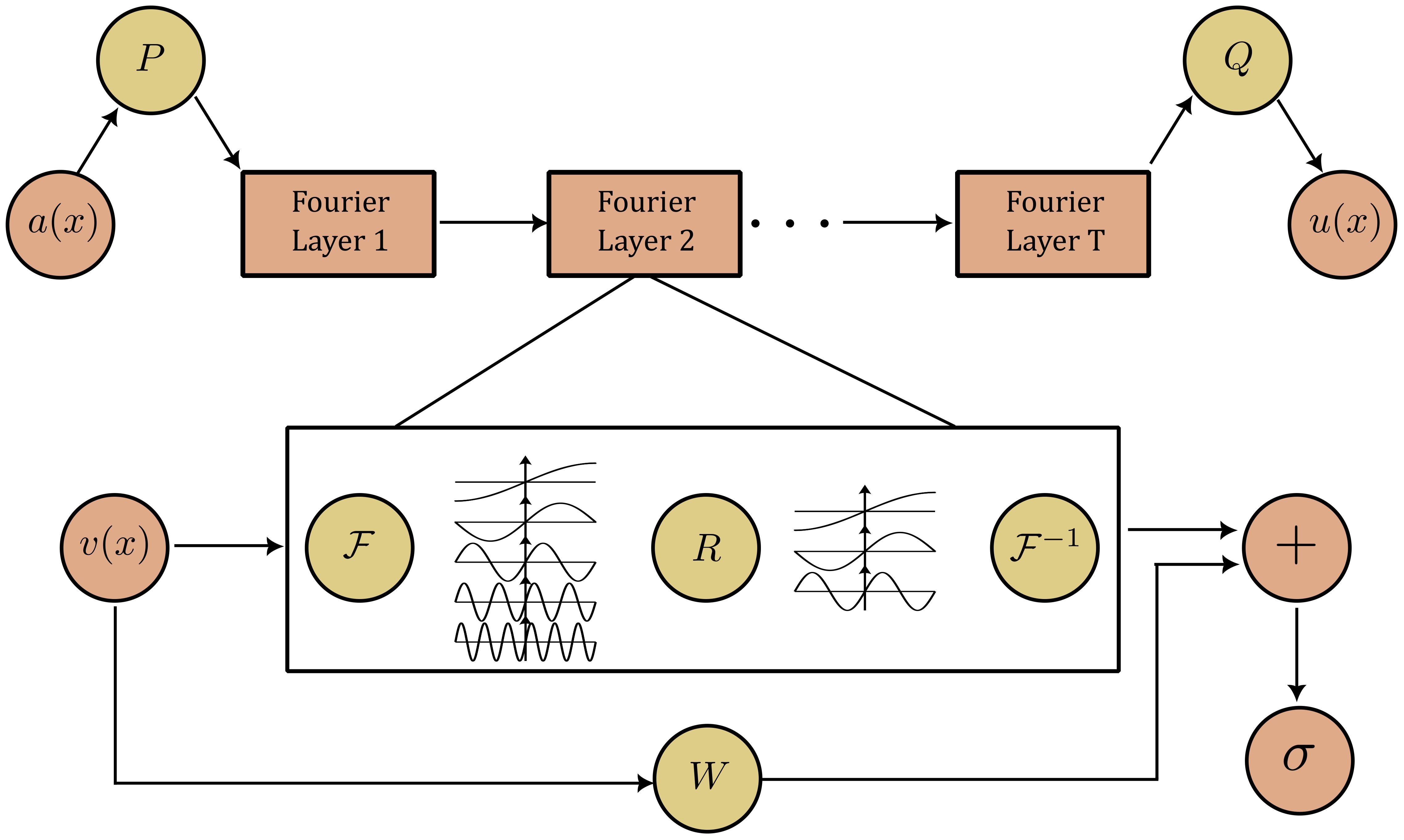
Figure 1 FNO architecture: a(x) and u(x) are input and output functions, P and Q are linear transformations, R and W are parameterization tensors and v(x) is computed by Equations (1)–(3).

First, the input function a(x) is lifted to a higher-dimensional space by a neural operator P as v₀(x) = P(a(x)). Next, the iterations $v_t\mapsto v_t{}_{+1}$ are performed by the non-linear maps

$\begin{array}{ll}{v}_{t+1}(x)=\sigma (W{v}_t(x)+K{v}_t(x)),& (1)\end{array}$

where σ is the non-linear activation function, W is the linear transformation, and K is the Fourier multiplier operator defined by

$\begin{array}{ll}K{v}_t(x)=F^{-1}(R·(F{v}_t)),& (2)\end{array}$

where R is some function in the Fourier domain and Φ and Φ⁻¹ are the Fourier and inverse Fourier transform, respectively. For the discrete case, R is expressed by the weight tensor $R\in {ℂ}^{k_{max}\times d_v\times d_v}$ and the multiplication is written efficiently as

$\begin{array}{ll}{(R·(ℱv_t))}_{k,l}={\displaystyle \sum _{j=1}^{d_v}{R}_{k,l,j}{(ℱv_t)}_{k,j},k\in {\mathbb{Z}}^d,\left|k_j\right|\le k_{max,j},}& (3)\end{array}$

where the number of Fourier modes in the jth direction is cut by k_max,_j. Thus, the neural operator is parameterized by the tensor R in the Fourier domain and by W in the space domain. Lastly, the output is the linear transformation of v_T by u(x) = Q(v_T(x)). Since the Fourier modes are cut and parameterized in frequency domain, the FNO is independent of input sizes.

For the purpose of solution operator learning of partial differential equations with time variable, two types of FNO architecture can be considered. The first type of FNO architecture, denoted by FNO3D, assumes all the variables equally. That is, the map a(x,t₀) → u(x,t) is learned by FNO3D in the space and time domains and the detailed explanation is given in Section 3. The next architecture type is the so-called recurrent FNO network and denoted by RFNO2D. The RFNO2D propagates along the time direction while performing the convolution operation in the space domain. In this paper, we chose two dimensions for the space domain so that FNO3D and RFNO2D perform Fourier transforms in 3D and 2D dimensions. Its full explanation is given in Section 4.

When the input is assumed periodic data, the FNO naturally processes it, as the Fourier transform (FT) is designed for periodic inputs. However, most of the data we encounter is non-periodic in nature. In the case of non-periodic inputs, the FNO networks adjust the bias term Wv_t(x) to the boundary values Equation (1) and learns the solution operator with high accuracy (Li et al., 2021). Note that the size of W is d_v × d_v and it is independent of the size of actual input a(x). Moreover, the input data are padded for the FNO networks if the non-periodic boundary condition is considered. Padding extends the input data dimensions by specific numbers (p) and sets the extended data portions to zero. After the main transforms (Fourier layers in our case) are performed, the extended dimensions are reduced back to its original dimensions. In this sense, for FNO networks, the padding helps to learn the boundary data. Therefore, zeros are padded to the extended grid points outside of the boundary in three dimensions for FNO3D networks and in two dimensions for RFNO2D. The effect of padding and its length is discussed in Section 5.

In the sequel, the root mean square error (RMSE), relative root mean square error (RRMSE), and anomaly correlation coefficient (ACC) are used to quantify the prediction performance and they are defined as:

$$\text{RMSE}=\sqrt{\frac{1}{N}{\displaystyle \sum _{i=1}^N{(f_i-o_i)}^2}}$$

$$\text{RRMSE}=\sqrt{\frac{{\displaystyle {\sum }_{i=1}^N{(f_i-o_i)}^2}}{{\displaystyle {\sum }_{i=1}^N{o}_i^2}}}$$

$$\text{ACC}=\frac{\frac{1}{N}{\displaystyle \sum _{i=1}^N(f_i-c_i)(o_i-c_i)}}{\sqrt{\frac{1}{N}{\displaystyle \sum _{i=1}^N{(f_i-c_i)}^2}}\sqrt{\frac{1}{N}{\displaystyle \sum _{i=1}^N{(o_i-c_i)}^2}}}$$

where N is the number of spatial points, f_i is the forecasted value, o_i is the observed value and c_i is the daily climatological mean value during the training period.

3 Double gyre ocean model and data acquisition for FNO learning

The simulation of the double gyre ocean circulation became the standard test bed for the number of purposes in oceanography and computational fluid dynamics. Starting from the very crude models (Stommel, 1948; Munk, 1950; Veronis, 1966), the double gyre ocean circulations have been studied extensively in the literature and they are rich enough in dynamics (Jiang et al., 1995; Pedlosky, 1996; Chang et al., 2001; Moore et al., 2004; Pierini, 2011). In order to prepare a large amount of simulation data in ocean circulations, we used the Regional Ocean Modeling system (ROMS). ROMS is a free-surface, terrain-following, primitive-equation ocean model widely used by the scientific community for a diverse range of applications (Haidvogel et al., 2000; Wilkin et al., 2005). In our simulations, most of the ROMS configurations and options were adapted from the test case reported in Moore et al. (2004). The ocean model is configured in the form of a flat-bottomed, rectangular ocean basin 1,000 km in longitude, 2,000 km in latitude, and 500 m in depth. The model consists of four equally spaced vertical levels of thickness 125 m. The primitive equations were solved on a mid-latitude β plane centered at 45°N with two different horizontal resolutions of 37 km and 18.5 km. With the Coriolis parameter β = 2 · 10⁻¹¹ m⁻¹ s⁻¹ and horizontal eddy viscosity 10 m² s⁻¹, the model circulation was forced by a stochastic wind forcing of the form

$\begin{array}{ll}{\tau }_x=(1+ϵ\widehat{r}(t))(-{\tau }_0)\text{cos }(2\pi y/L_y),& (4)\end{array}$

where τ₀ = 0.05 Nm⁻², L_y = 2,000 km is the meridional extent of the basin, and $\widehat{r}(t)=r(t)/{\sigma }_r$ is wind-noise with unit variance. With the standard deviation σ_r, r(t) is the solution of the Ornstein–Uhlenbeck stochastic differential equation

$\begin{array}{ll}\frac{dr}{dt}=-ar+b\eta ,& (5)\end{array}$

where η is a Gaussian white noise with unit variance and zero mean and a and b are positive constants. In order to discretize the Equation (4), we need to discretize the Equation (5). The discretized version of Equation (5) is written as

$\begin{array}{ll}{r}_{k+1}=\alpha r_k+\beta {\eta }_k,& (6)\end{array}$

where α = (1 − aΔt) and β = bΔt. It is known that the solution of Equation (6) with α = 0 is a Gaussian white noise whereas α = 1 corresponds to a Wiener process. One can obtain different realizations of a red noise by adjusting the parameter α in the range (0,1]. To include the atmospheric variability in our model, we choose the values α = 0.9, ϵ = 0.025, and β = 1 with Δt = 1 day. These parameter values are chosen based on the study of coherence resonance in a double gyre model by Pierini (2010). In addition, to generate non-linear instability and different turbulent regimes, the initial values of the velocity components u,v and w were generated by the Gaussian random fields, in which the random perturbations are given in the Fourier domain as depicted in Evensen (1994). Starting from the random initial state, the model was run for 1,800 days as shown in Figure 2. The same simulation was repeated 40 times resulting in different final states caused by the random initial states, the atmospheric variability, and the turbulent nature of the flow. Furthermore, the 1,800 days of each simulation was divided into 30 intervals of length 60 and we obtain a total of 1,200 instances. Thus, our data have the dimension 1,200 × 3 × m × n × 60, where three features are horizontal velocity components (u,v) of the upper layer and the ocean surface height (ζ) and m × n is the number of horizontal grids. Since FNO learns mapping from a(x) to u(x), the data are divided into two sets of the shapes 1,200 × 3 × m × n × T_in and 1,200 × 3 × m × n × T_out, where T_in and T_out are the input and output time dimensions and the conditions T_in + T_out ≤ 60 and T_in ≤ T_out are satisfied. The latter condition is to satisfy a precondition for solution operator mapping. That is, given the point a(x) = u(x,t₀), FNO3D gives the latter values of solutions u(x) = a(x,t) for t ≥ t₀. Out of 1,200 instances, the first A FNO3D network 1,000 are taken as training data and the remaining 200 are used for testing and validating. In each simulation, the first 10 days are the spin-up time for the model’s circulation to reach a physical solution.

Figure 2

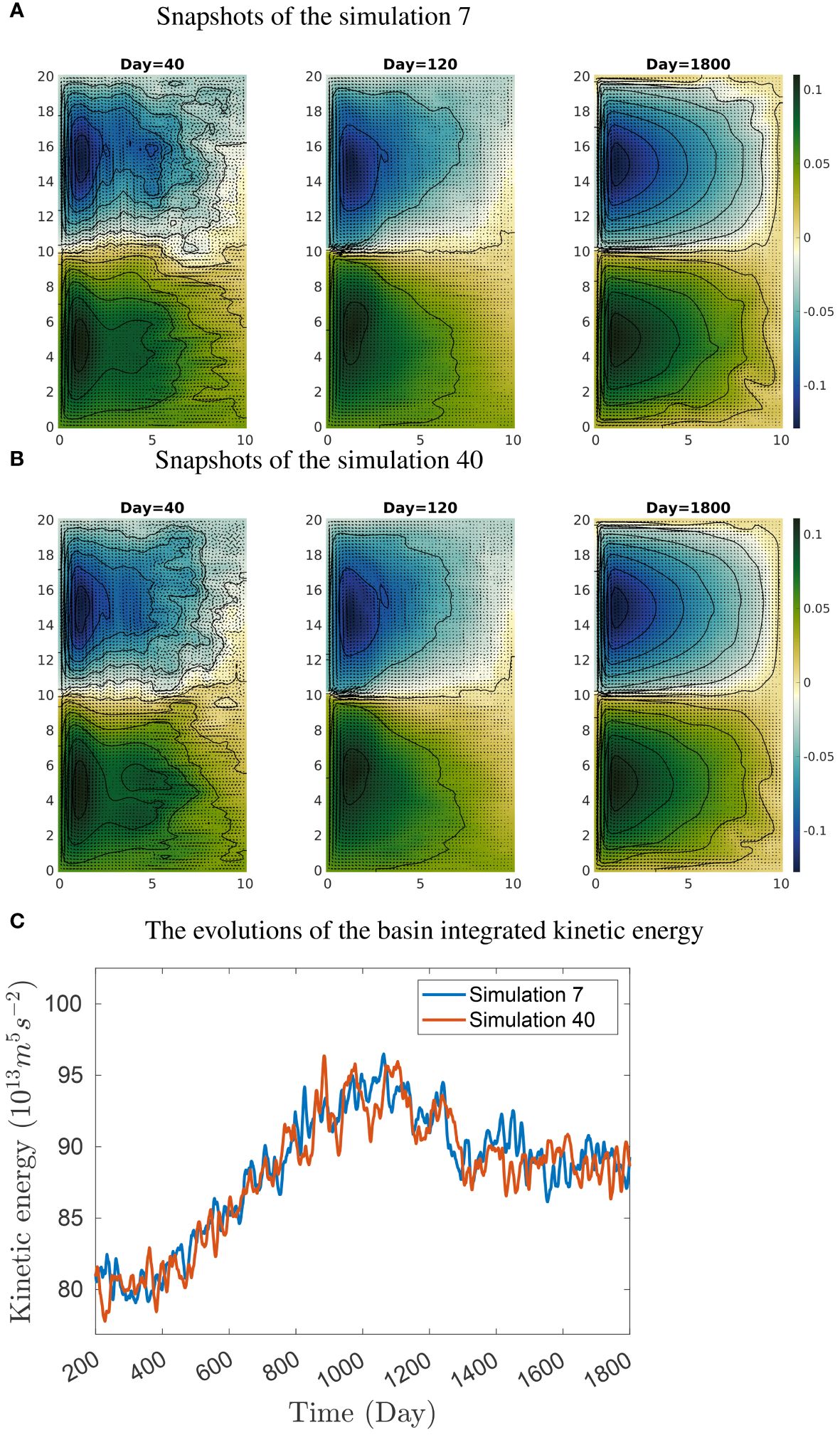
Figure 2 (A, B) ROMS simulation snapshots of the sea surface height ζ (color shading in meters) and horizontal current vectors (u,v) of the upper layer of the double gyre circulations at different times (axis unit: 10⁵ m). (C) Variation of basin-integrated kinetic energy change in simulations 7 and 40.

The overall FNO3D structure is presented in Figure 3A, and the hyperparameters are T_in = 10, T_out = 40, d_v = 20, k = 128, and k_max,_j = (14,28,8). The input data have the shape b×f ×m×n×T_in and; for simplicity, the notation (A,B) indicates that A is the input and B is the output of the component, so the overall output of the FNO3D network is of the shape b × f × m × n × T_out. It means that the FNO3D network predicts the last T_out time data snapshots based on the previous T_in data. Note that, although it is not explicitly shown in the flow diagram, the input data are accompanied by the spatial and temporal grid information.

Figure 3

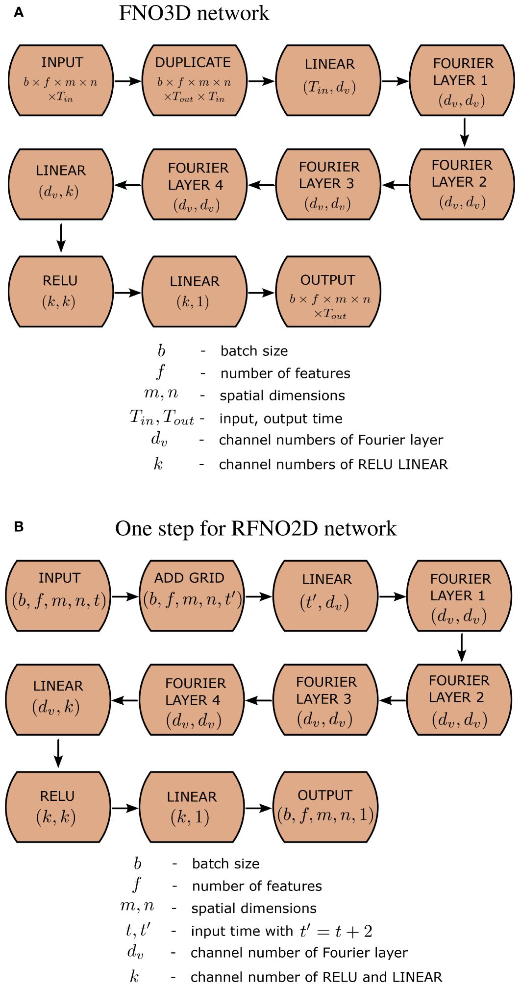
Figure 3 The data flow diagram of FNO networks. (A) FNO3D network and (B) RFNO2D network.

3.1 Training and testing FNO model for double gyre ocean circulations

In this section, we present the results of training and testing processes of FNO3D models. Two horizontal grid systems m × n = 27 × 54 and m × n = 54 × 108 are considered for testing the mesh independence property of the FNO3D model, and we denote them by FNO3D_27×54 and FNO3D_54×108 the corresponding neural networks. Four Fourier layers with the ReLU activation as in Figure 3A were chosen, and the Adam optimizer with the RRMSE loss function, learning rate 0.001, step 100, number of epochs 500, and batch size of 20 was set. We chose 3D padding as (6,6,6). Putting k_max,_j = (14,28,8) and d_v = 20 yields 120,427,177 learnable parameters for both FNO3D_27×54 and FNO3D_54×108. All the computations are carried out on a computer with NVIDIA A100 80GB GPU housed at the Korea Institute of Science and Technology Information center (www.kisti.re.kr).

For the steady wind case (ϵ = 0), the final achieved test errors (RRMSE) of FNO3D_27×54 and FNO3D_54×108 are 0.009 and 0.020, respectively. All the presented error values are combined over the features u,v,ζ and averaged over the batch number and the training or test samples. Note that the error from the model trained on finer resolution data is slightly higher than the lower-resolution model. It may be seen in contrast with the traditional solvers such as finite difference and finite element methods, where numerical models with finer discretization yield lower errors. This is because the number of learnable parameters is the same for both FNO3D_27×54 and FNO3D_54×108 models. Therefore, when the resolution of the training data is increased, it is expected that the model needs to learn more turbulent flow dynamics. The same applies to RFNO2D models. However, when the stochastic wind force is introduced (ϵ = 0.025), the RRMSE of FNO3D_27×54 and FNO3D_54×108 models are 0.032 and 0.026, respectively. These errors, which are in contrast with the steady wind case, tend to grow as the intensity of randomness ϵ increases. Since the same randomness and intensity is applied to both models, it is observed that lower-resolution model FNO3D_27×54 resolves less variability so the error becomes slightly higher than that of the higher-order model.

Recall that, in our simulation, the input data into the FNO3D network have the dimension 3 × m × n × 10 (excluding batch) and the output has the shape 3 × m × n × 40. In Figure 4, we present the visual comparison of actual values and the output of trained nets for the last snapshot (i.e., 40th). Figure 4B shows the output of FNO3D_54×108, and Figure 4C shows the output of FNO3D_27×54, which is trained on 27 × 54 resolution data and applied to 54 × 108 resolution. The comparison of u,v and ζ for the same time point is given in Figures 4D-F. We almost cannot find the differences visually between the predicted and the actual solution. For this resolution-free comparison, the RRMSE of the prediction by FNO3D_27×54 and FNO3D_54×108 are 0.065 and 0.033, respectively. While the approximate time spent on obtaining 40-day snapshots by ROMS at four parallel processes is 36.8 s, the same 40-day evaluation of FNO3D takes 0.00596 s.

Figure 4

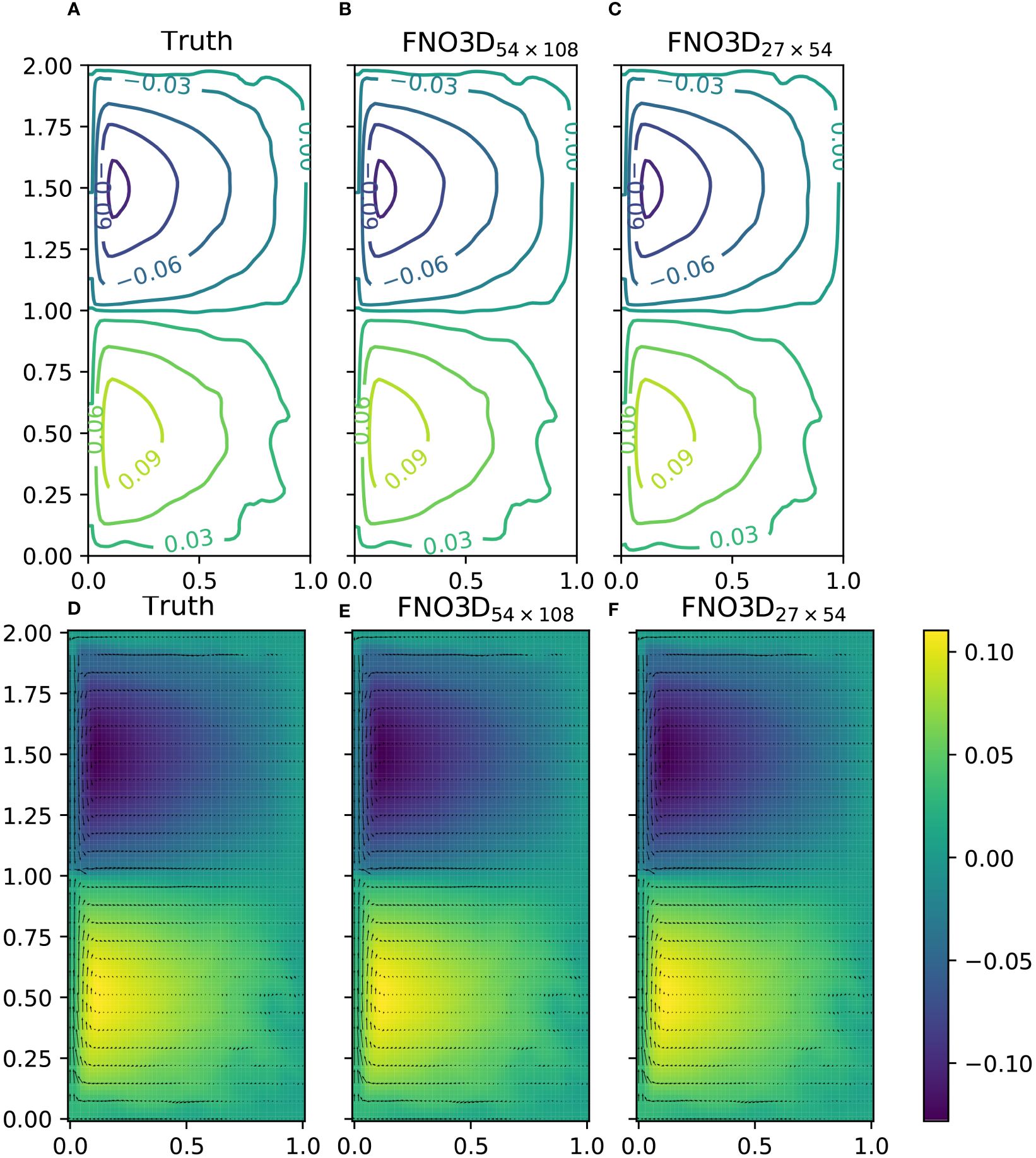
Figure 4 Comparison of u,v and ζ values on 54 × 108 mesh for ν_h = 10 m² s⁻¹ (axis scale ×10⁶ m). (A, D) The actual solution. (B, E) The output of FNO3D_54×108, which is trained and applied to 54 × 108 resolution. (C, F) The output of FNO3D_27×54, which is trained on 27×54 resolution but applied to 54×108 resolution. (A-C) Contour lines of ζ. (D, E) Quiver plot of u,v and ζ values (colored).

There is not much variation in the kinetic energy of the double gyre model after 1,200 days (Figure 2). However, out of 1,200 instances, 1,000 instances were used for training, as detailed in the beginning of Section 3, whereas the remaining 200 instances were reserved for testing. These 200 instances contain approximately six sets of double gyre ocean state evolutions. Each set includes ocean states from the initial state on day zero to the end of simulation on day 1,800. Consequently, the reported test set RRMSEs are averaged over the entire evolutions of double gyre ocean circulation, including both non-equilibrium states and quasi-steady states (Figure 2).

Finally, we give the brief comparison of FNO3D and RFNO2D for the double gyre ocean circulation learning task. The full description of RFNO2D is given in Section 4.2 by Equations (7)–(11). Overall, the performances of FNO3D and RFNO2D are comparable with the same learning parameters and 2D padding (6,6). For the viscosity ν_h = 10 m²/s, the RRMSEs of the 10-day input and 40-day output (10d–40d) predictions of RFNO2D_27×54 and RFNO2D_54×108 are 0.039 and 0.041, respectively.

While the training time for the RFNO2D network is longer than the FNO3D counterpart, the number of learnable parameters of the RFNO2D network is significantly less than that of the FNO3D network. We present the averaged RMSE comparison of FNO3D and RFNO2D networks for the first 50 instances of the test set in Figure 5. For both FNO3D and RFNO2D networks, the prediction errors of velocity components are higher than that of the ocean surface height and continue to increase as the time increases. However, the errors for the ocean surface height remain relatively stable. This supports the fact that the flow velocity is more challenging to model compared with other ocean variables. We see that the performance of RFNO2D is slightly better than that of FNO3D. Another advantage of the RFNO2D network compared with FNO3D is that it requires less memory for the implementation, since it advances by one time step whereas FNO3D saves whole time interval data in the memory. Although not shown in this paper, from another comparison, we found that the prediction accuracy of RFNO2D was better than that of the persistence model.

Figure 5

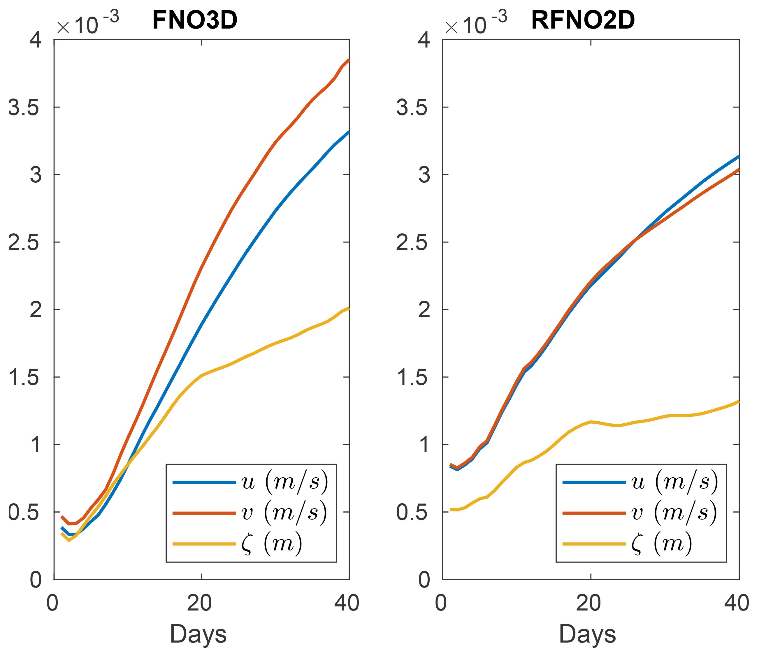
Figure 5 RMSE comparison of FNO3D and RFNO2D predictions for the first 10 instances of test data (ν_h = 10 m² s⁻¹, m × n = 54 × 108).

4 Predictions of a circulation in the East Sea by FNO networks

In this section, we apply RFNO2D networks to the prediction of a regional ocean circulation in the EJS.

4.1 Data acquisition and processing

Bounded by Japan, Korea, and Russia, the EJS is of great scientific interest as a semi-enclosed “small ocean”. Its basin-wide circulation pattern, boundary currents, subpolar front, mesoscale eddy activities, and deepwater formation are similar to those in an open ocean. The HYCOM.org provides access to near-real-time global ocean prediction system output. The HYCOM data are essentially reanalysis dataset that is the result of optimal combination of observation and numerical ocean model (data assimilation). Although several combinations of ocean prognostic variables are available, we select three important and challenging variables: ocean current velocities u and v at 10 m below from the ocean surface and sea surface height ζ. The data have 0.08° lon × 0.08° lat resolution and covers the 1994–2022 time interval. Although it is possible to consider the whole domain of EJS in our computation, the most circulation dynamics are occurring in the southern region, where the subpolar front is formed and fluctuating. Moreover, including the whole EJS in the learning task increases the grid dimension inefficiently as greater part of it consists of land.

Extracting only ocean grid cells in the EJS part by converting 2D data to 1D data may be considered; however, we observed that doing so loses spatial dependence significantly and results in poorer performance for our FNO learning task. Therefore, we chose the southern part of EJS enclosed by 36.48°N–40.76°N, 128.96°E–139.12°E coordinates as our computation domain (Figure 6). For the land part of the domain, we set the velocity components to zero and ζ to the value $\overline{\zeta }=0.065$, the mean over the considered domain. The time variability of the considered variables at the coordinate 38°E, 132°N, is depicted in Figure 7. The mean values of velocity components are $\overline{u}=0.036m/s$ and $\overline{v}=0.013m/s$, and the three variables (u,v,ζ) fluctuate in the ranges of −1.11–1.17, −1.39–1.18, and −0.61–0.81, respectively. The seasonal variability of ζ is more evident than that of other variables. The time interval ranging from 1994/01/01 to 2022/12/31, that is, 10,592 days, is divided to the 50-day interval with the 5-day stride thus excluding the last 2 days. Thus, our data have the shape 2,109 × 3 × 128 × 64 × 50, where it indicates 50 days, 128 × 64 spatial resolution, three features (u,v,ζ), and 2,109 instances of data. Out of 2,109 instances, the first 1,900 instances are chosen as the training set and the last 200 instances are taken as the test-1 set (see Table 1). On 18/02/2020, HYCOM discontinued the grid GLBv0.08 that had the resolution 0.08° lon × 0.08° lat. While the data after 2020/02/18 for test 1 are interpolated to match the original resolution, the test 2 data are prepared for the new resolution 0.08° lon × 0.04° lat to check the resolution-free evaluation of FNO networks. Since the training and test sets are not overlapped, the evaluation result of a trained model on test sets can be seen as the prediction of the future states of the EJS.

Figure 6

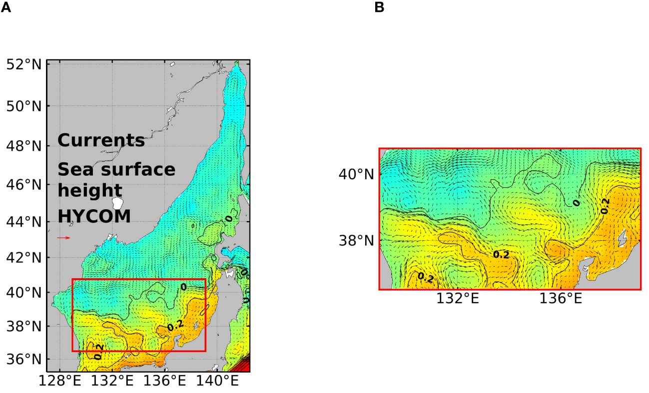
Figure 6 (A) Distribution of currents (u,v) at a depth of 10 m and sea surface height (ζ) in the East/Japan Sea on 2018/12/07. (B) The domain of study (magnified).

Figure 7

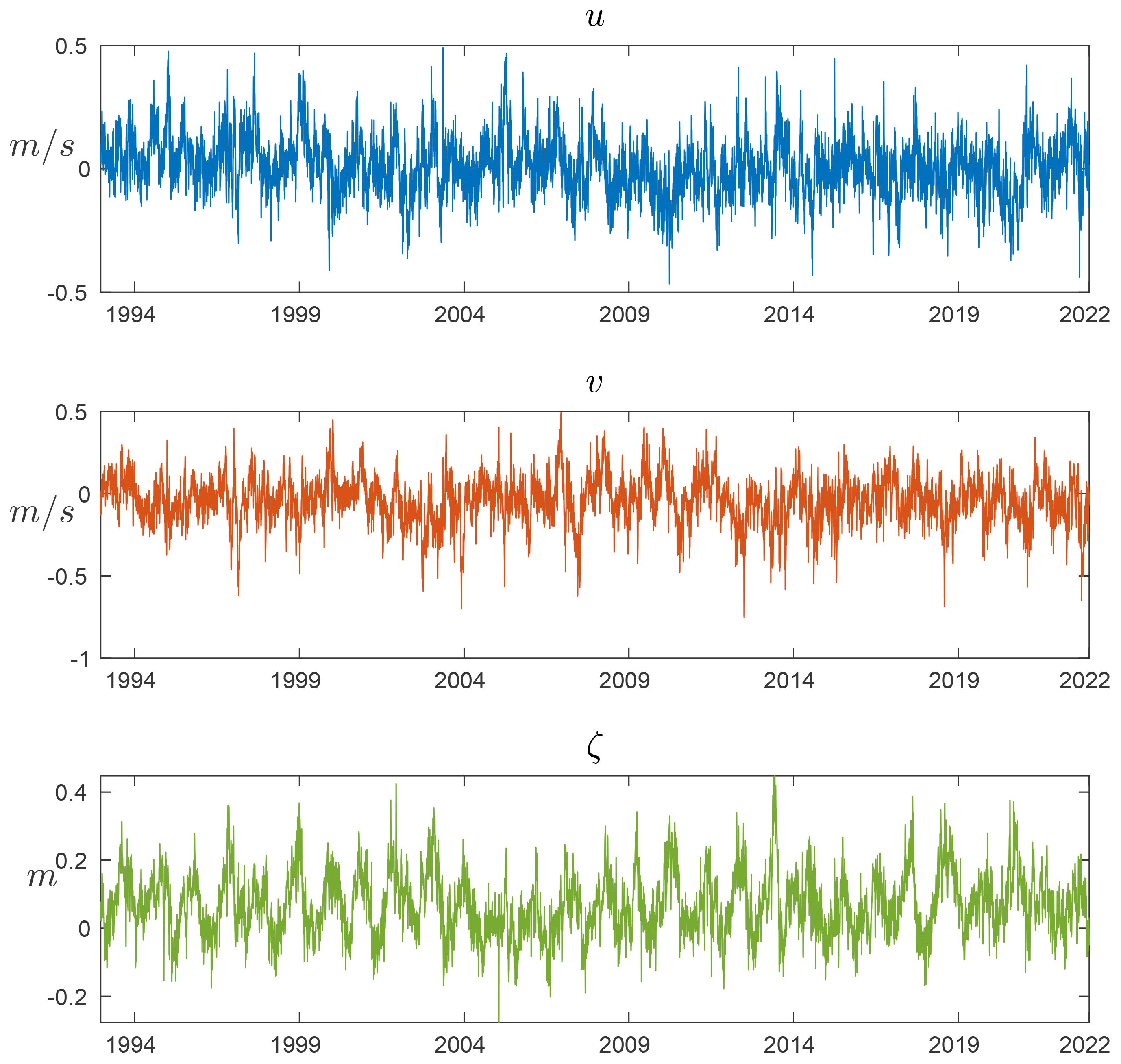
Figure 7 Time series of daily mean u,v and ζ at 38°E, 132°N in the East/Japan Sea from 01/01/1994 to 31/12/2022.

Table 1

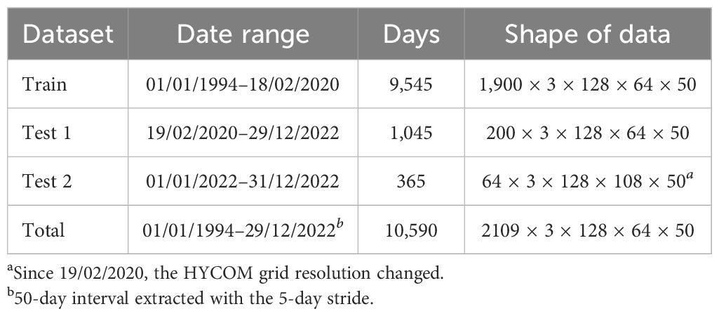
Table 1 Training and test data for the prediction of the regional ocean circulation in EJS.

4.2 Training and testing

For the prediction task of EJS model variables, we use the recurrent version of the original FNO networks with the additional features and the data flow diagram of RFNO2D is given in Figure 3B. First, the RFNO2D network with the three features u,v,ζ takes the t consecutive days data as input and predicts the next-day states. The RFNO2D network performs Fourier transform along the spatial domain (2 in our case); hence, the name RFNO2D is given. The output of the RFNO2D is augmented to the input of the next prediction. With the notation Φ_k = (u_k,v_k,ζ_k), the recurrent RFNO2D network propagates along time dimension as depicted in Equations (7)–(11). Thus, given the input data (Φ₁,Φ₂,…,Φ_t), the recurrent RFNO2D network predicts the next s day states (${\widetilde{\text{Φ}}}_{t+1},{\widetilde{\text{Φ}}}_{t+2},\dots ,{\widetilde{\text{Φ}}}_{t+s}$). Let us denote the above task td-sd prediction in the sequel.

For t = 5, s = 5, the computation flow is as follows:

$\begin{array}{ll}{\widetilde{\text{Φ}}}_6=\text{FNO}2\text{D}({\text{Φ}}_1,{\text{Φ}}_2,{\text{Φ}}_3,{\text{Φ}}_4,{\text{Φ}}_5)& (7)\end{array}$

$\begin{array}{ll}{\widetilde{\text{Φ}}}_7=\text{FNO}2\text{D}({\text{Φ}}_2,{\text{Φ}}_3,{\text{Φ}}_4,{\text{Φ}}_5,{\widetilde{\text{Φ}}}_6)& (8)\end{array}$

$\begin{array}{ll}{\widetilde{\text{Φ}}}_8=\text{FNO}2\text{D}({\text{Φ}}_3,{\text{Φ}}_4,{\text{Φ}}_5,{\widetilde{\text{Φ}}}_6,{\widetilde{\text{Φ}}}_7)& (9)\end{array}$

$\begin{array}{ll}{\widetilde{\text{Φ}}}_9=\text{FNO}2\text{D}({\text{Φ}}_4,{\text{Φ}}_5,{\widetilde{\text{Φ}}}_6,{\widetilde{\text{Φ}}}_7,{\widetilde{\text{Φ}}}_8)& (10)\end{array}$

$\begin{array}{ll}{\widetilde{\text{Φ}}}_{10}=\text{FNO}2\text{D}({\text{Φ}}_5,{\widetilde{\text{Φ}}}_6,{\widetilde{\text{Φ}}}_7,{\widetilde{\text{Φ}}}_8,{\widetilde{\text{Φ}}}_9)& (11)\end{array}$

The parameter selection is presented in Table 2, and the training process is stopped after the test 1 error started to increase with patience number 10. First, in order to determine the performance dependence of the input length and the output length, we considered three types of prediction tasks: T = 10, T = 25, and T = 30, where we denote by T the total length of time T = T_in +T_out. For T = 10, three different models with 5d–5d, 7d–3d, and 9d–1d are trained and the test errors are given in the Table 3A. Comparing these three types of prediction tasks, there is no significant performance gain for increasing input and decreasing output with a fixed total number of days T = 10. It means 5-day input is the optimal setting for the chosen RFNO2D structure and parameters, since smaller number of days as input can make a longer prediction with similar performance as applying more days as input. Second, we tested the error dependence on the total time T. For the case T = 25 as shown in Tables 3B–D, the best configuration was for 15d–10d. Increasing the input length as in Table 3E to T_in = 20 does not improve the error. In general, the test error increases as T is increased. Therefore, we prefer 5d–5d configuration for short time prediction and 15d–10d for longer time prediction. In the sequel, we considered the 15d–10d prediction task and denoted the trained model by RFNO2D_128×64. Here, 128 × 64 is the horizontal spatial dimension on which the RFNO2D is trained.

Table 2

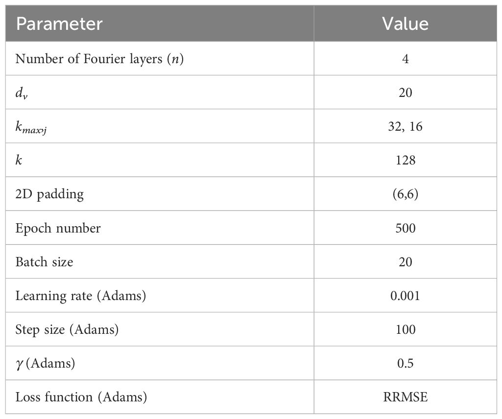
Table 2 Parameter selection of RFNO2D for the regional ocean circulation predictions in the southern EJS.

Table 3

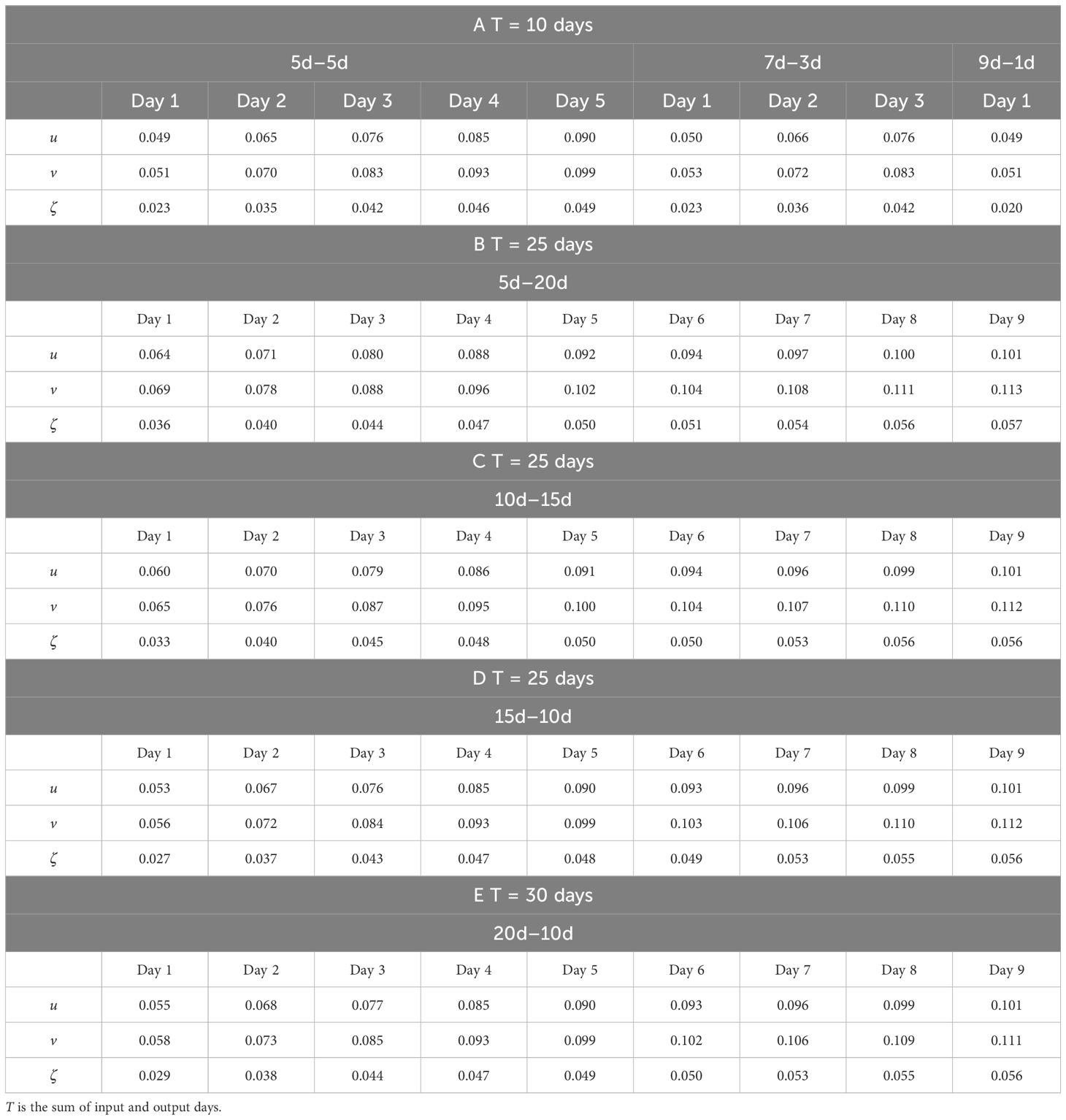
Table 3 Mean RMSE of u, v and ζ for the test 1 dataset.

We present the RMSE and the ACC in Figure 8 for the trained RFNO2D_128×64 validated on the test 1 dataset. The RMSEs in surface currents (u and v) show a rapid increase from the first prediction day to the fifth day, after which the rate of increase gradually diminishes (Figure 8A, Table 3). Similarly, the RMSE in sea surface height (ζ) exhibits a rapid increase from the first prediction day to the fourth day. Additionally, the ACC follows a similar tendency: as the prediction day progresses; the ACCs linearly decrease for the initial 4–5 days (Figure 8B). There are extreme peaks in RMSEs in the prediction of surface currents on specific dates, such as 27/08/2020 (test number 38), 08/08/2021 (test number 108), and 05/09/2022 (test number 187). On those day, Typhoons Bavi, Lupit, and Hinnamnor traversed the Yellow Sea, the East China Sea, and the EJS, respectively, with strong winds prevailing over the EJS. Given that the RFNO2D_128×64 network does not incorporate the effects of extreme winds caused by typhoons during the prediction process, it is likely that prediction errors are significant during these periods.

Figure 8

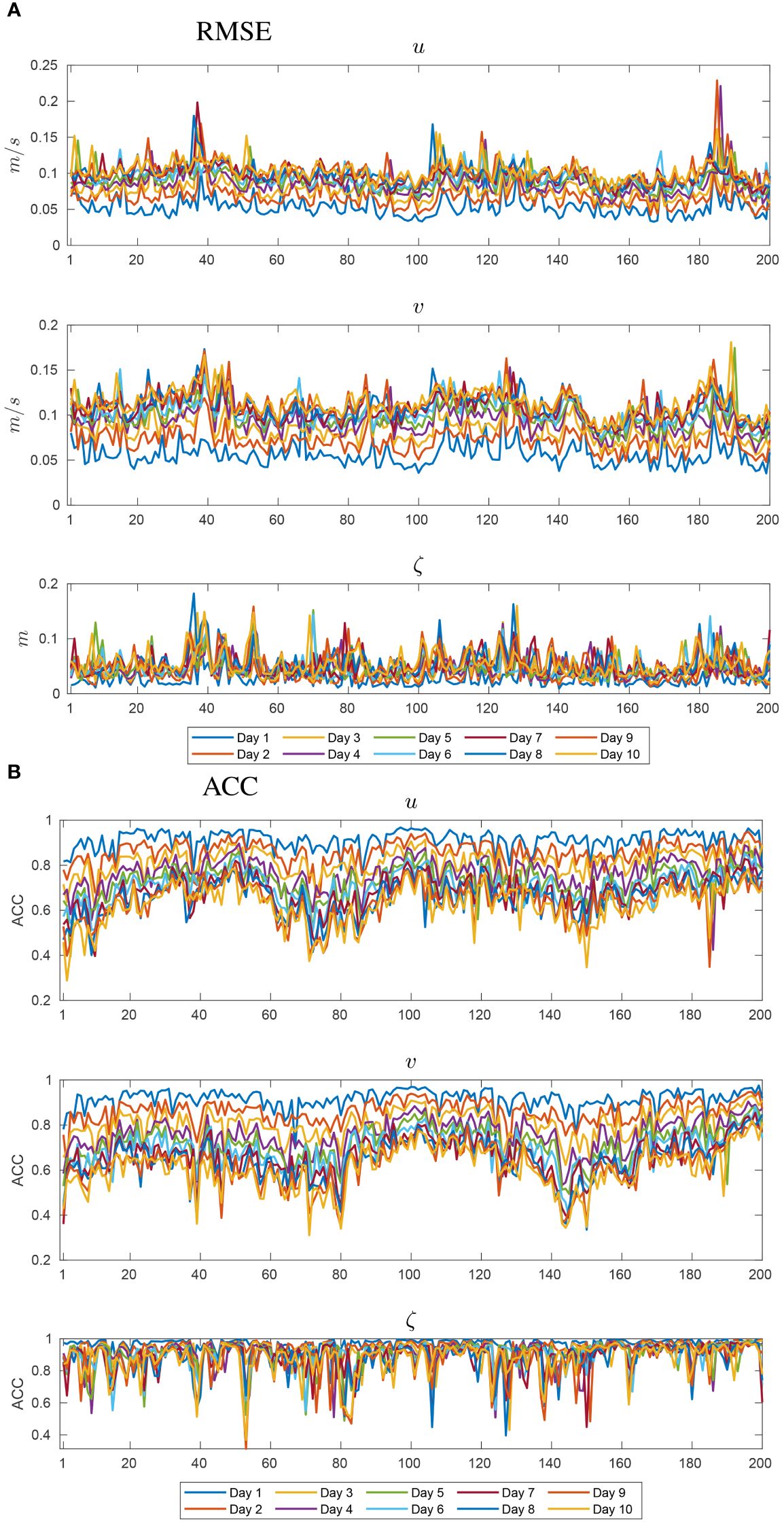
Figure 8 (A) The RMSE and (B) the ACC of surface current (u and v) and sea surface height (ζ) predicted by the RFNO2D_128×64 with 15-day input and 10-day output (15d–10d) in the southern EJS for the test 1 dataset. The horizontal axis denotes test number for 200 instances (Table 1).

Next, the forecasting ability of RFNO2D_128×64 is compared with that of the persistent and vector auto-regression (VAR) models, which are assumed as baseline models. For the 15d–10d prediction task, the persistent model assumes that the next 10 days’ values are the same as the last input day’s value. That is, given the 15-day input Φ₁,Φ₂,…,Φ₁₄,Φ₁₅, the prediction of next 10 days is

$${\widetilde{\text{Φ}}}_{16}={\widetilde{\text{Φ}}}_{17}=\dots ={\widetilde{\text{Φ}}}_{25}={\text{Φ}}_{15}.$$

The VAR is a statistical model that captures the linear relationship of multiple variables as they change over time. In our notation, the VAR(p) model with p lags is written as

$${\widetilde{\text{Φ}}}_t=c+A_1{\text{Φ}}_{t-1}+A_2{\text{Φ}}_{t-2}+\dots +A_p{\text{Φ}}_{t-p}+e_t,$$

where c is a constant vector with dimension 3, A_k is the time-invariant 3 × 3 matrix, and e_t is the error term. The VAR(p) model estimates next days’ values by propagating along time dimension similarly as in Equations (7)–(11). We chose the Φ_k = (u_k,v_k,ζ_k) values at the coordinate 38°E, 132°N in the EJS as depicted in Figure 7. For the fair comparison, the maximum lag should be less than 15. The Adfuller test confirmed the stationarity of our time series, and, surprisingly, the Akaike information criterion (AIC) took the minimum value at lag p = 15 when tested for optimal lag in the range from 1 to 20. The performance comparisons of RFNO2D_128×64, persistent, and VAR(15) models are shown in Figure 9 where the prediction RMSE is averaged over the test 1 set and graphed against the prediction days from 1 to 10. Generally, RFNO2D_128×64 outperforms these baseline models. The persistent model prediction, as expected, yields higher error than the other two methods for all the variables. While the prediction ability of the u component by RFNO2D_128×64 is persistent along the prediction days, starting from the sixth day, RFNO2D_128×64 and VAR(15) perform similarly on the v component. We believe the reason is that surface currents generally flow eastward or northeastward and the v component carries more uncertainty than the u component. For the ζ variable, the two models RFNO2D_128×64 and VAR(15) are in competitive manner or on par with each other.

Figure 9

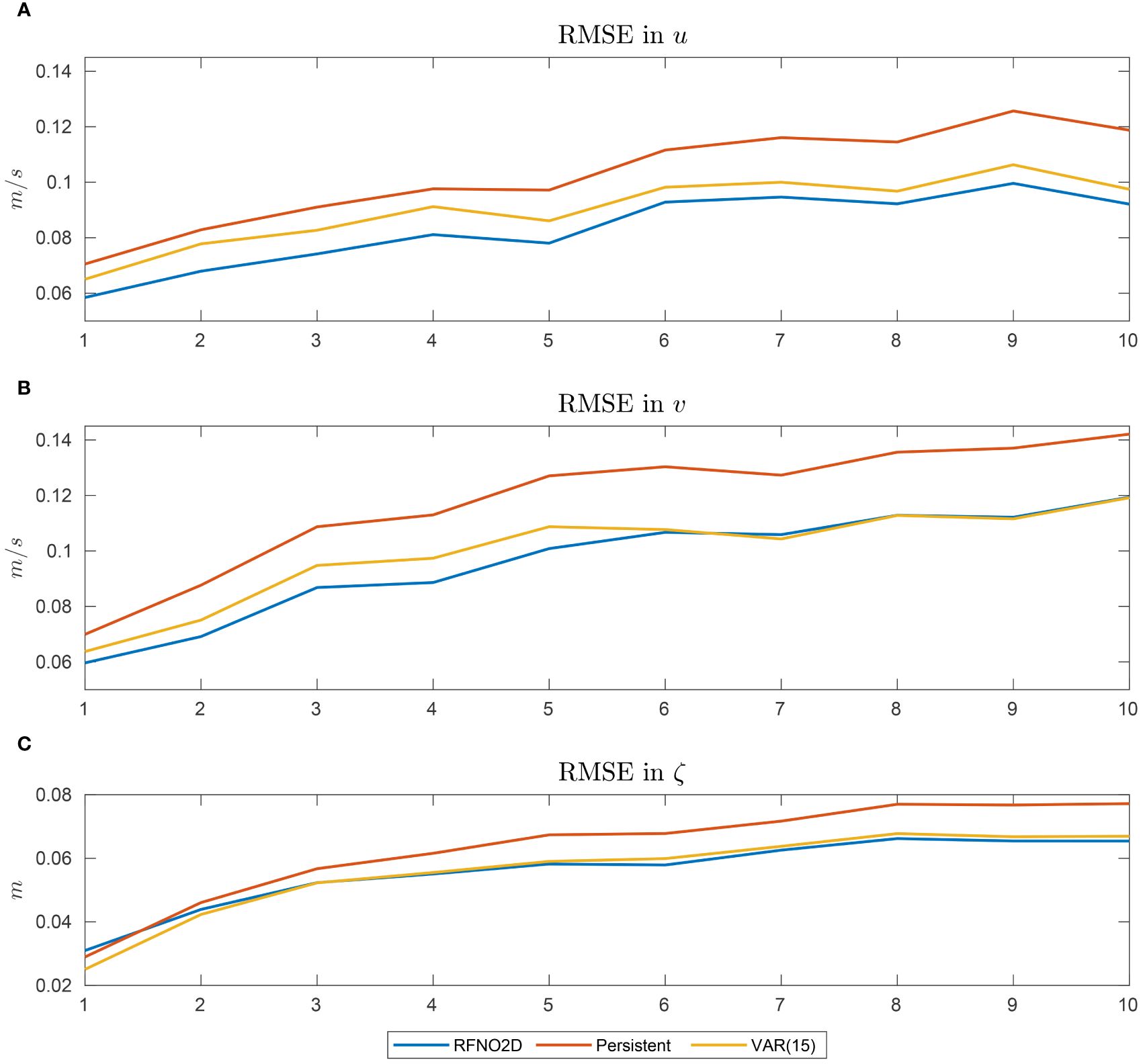
Figure 9 Performance comparison of RFNO2D_128×64, persistent, and VAR(15) models for 10 prediction days. RMSE in (A) u, (B) v, and (C) sea surface height.

In Figure 10, the comparison of 15d–10d prediction on the 1st, 2nd, 4th, 7th, and 10th days starting from 17/08/2022 is given in the form of surface current field and sea surface height ζ. The East Korea Warm Current (EKWC) is vigorously meandering with four wave crests (troughs) extending from the west to east. The surface current at a depth of 10 m predominantly flows northeastward toward the Tsugaru Strait (Figure 10). Anti-cyclonic eddies tend to form to the south of the EKWC, whereas cyclonic eddies typically develop in the northwest region of the domain. During the initial 2 days of the prediction, the surface current speed and the meandering patterns of surface currents and the locations of eddies in the predictions closely match the truth. However, starting from day 4 (20/08/2022), the surface current speed appears slightly weaker in the prediction compared to the truth, despite similar meandering patterns of surface currents and the locations of eddies. These differences may originate from relatively strong southwesterly winds from August 19 to 20, with daily speed of 5.1 m/s–6.3 m/s. From August 17 to 18, daily wind speeds measured at Ulleung Island (130.90°E, 37.48°N) were 1.4 m/s to 2.1 m/s. It is noteworthy that the FNO model does not have information on wind for the prediction.

Figure 10

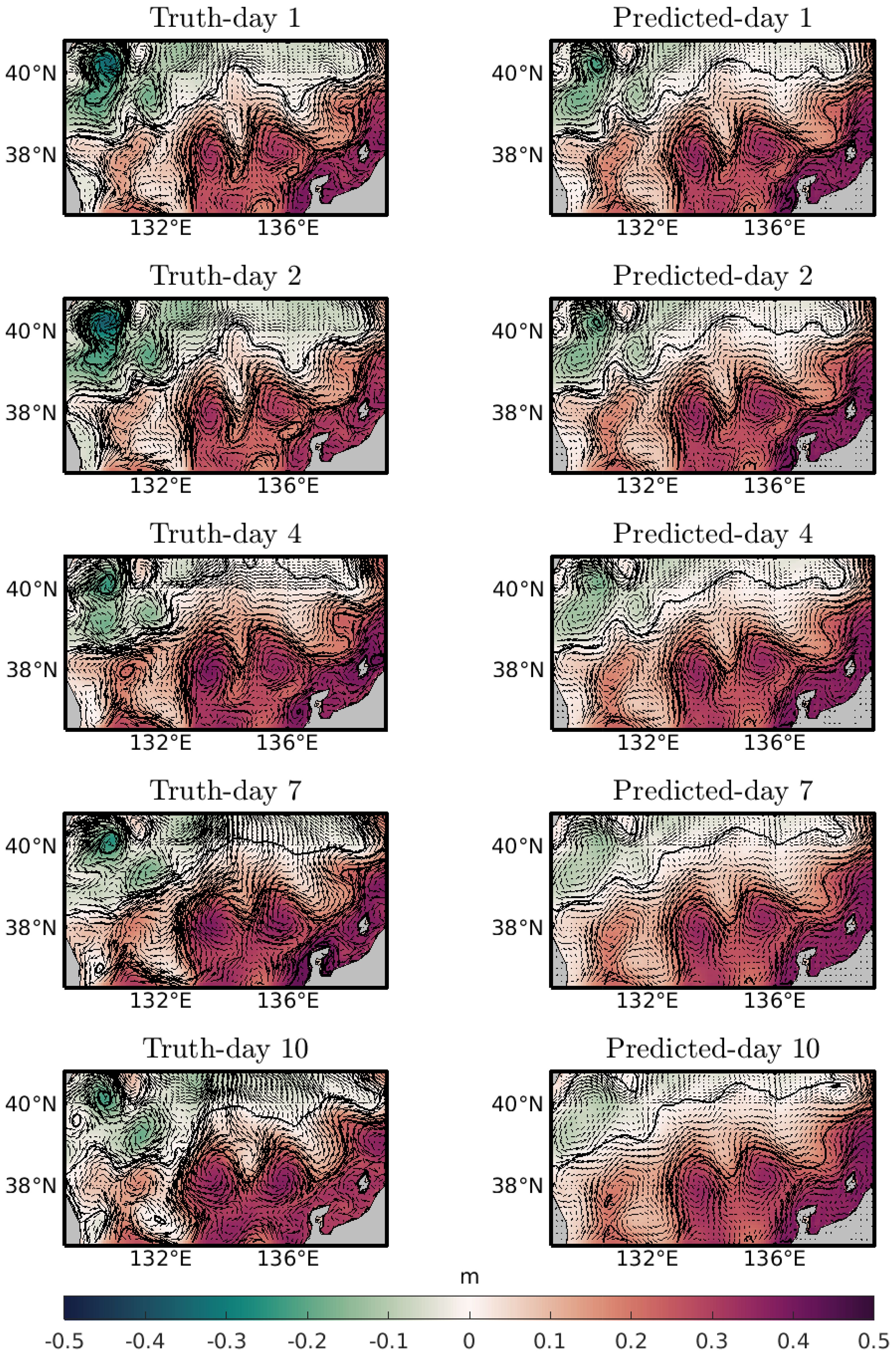
Figure 10 Comparison of truth and predicted variables for 17/08, 18/08, 20/08, 23/08, and 26/08/2022. Color represents the sea surface elevation in m, and black vectors are currents at a depth of 10 m. Contour interval is 0.2 m.

Note that the model RFNO2D_128×64 is trained on 128 × 64 resolution data. Since the FNO networks are independent of input grid size, we evaluated the RFNO2D_128×64 network on test 2 dataset, which has a 128 × 108 grid system, and the differences between the predicted values and the truth are given in Figure 11. This demonstrates the resolution-free property of the FNO network. Even when surface currents and sea surface height are predicted on a finer grid system, errors remain relatively small during the initial 2 days. However, the errors (predicted – truth) increase for all variables from the first prediction day to the fourth day. The errors in v did not propagate horizontally but instead statically grew over time. The differences in u gradually increased from the first day to the fourth day. Afterward, the error in u oscillated in time from the 7th day to the 10th day.

Figure 11

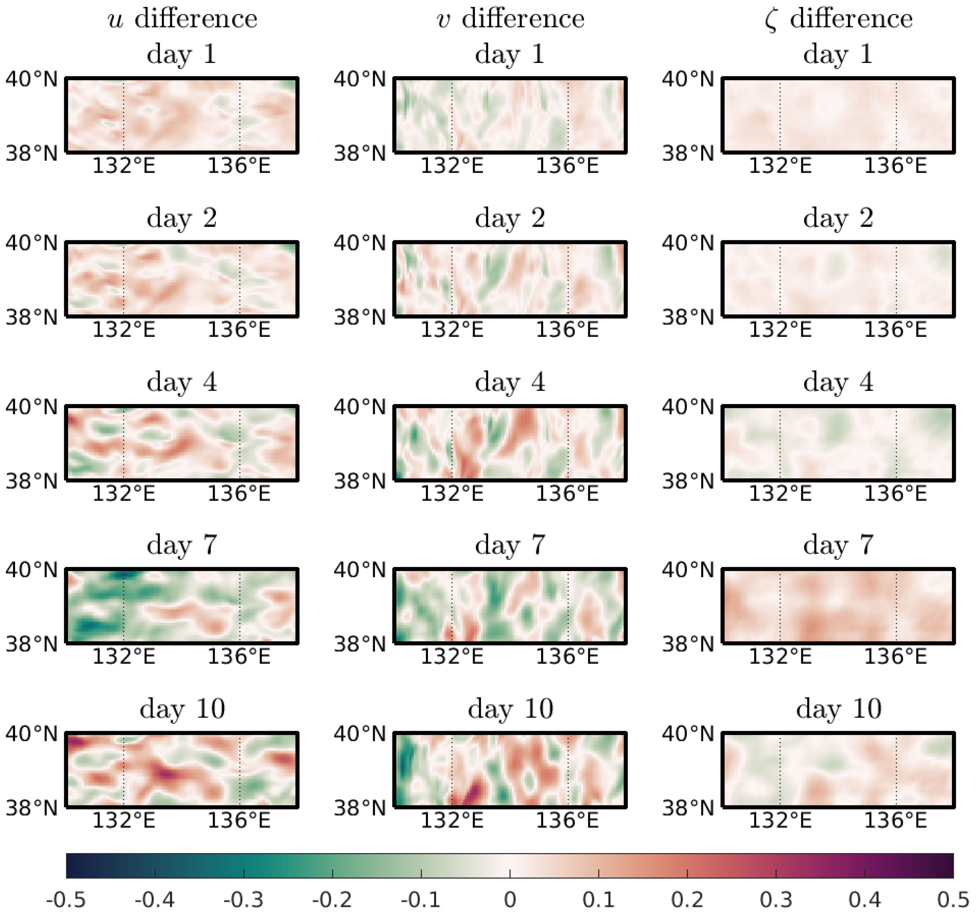
Figure 11 Horizontal distribution of daily error (predicted-truth) in u,v and ζ from 07/11 to 16/11/2022. The model RFNO2D_128×64 was trained on the 128 × 64 grid and evaluated on a 128 × 104 resolution for 15d–10d prediction. Units of velocity components (u and v) and sea surface height (ζ) are m/s and m, respectively.

5 Discussion and conclusion

In this paper, we applied the deep learning algorithm inspired by the FNO to the ocean prediction problem in the framework of the double gyre ocean circulation model and a regional circulation model for the East/Japan Sea. For the double gyre ocean circulation model, the FNO network learns the solution operator of the governing primitive equations forced by the stochastic surface wind stress in the form. To prepare a large amount of training and testing samples, we run the Regional Ocean Modeling System with the initial data generated by the random Gaussian fields. Extensive numerical tests show that, once learned, the FNO3D and RFNO2D networks predict the ocean states with a high accuracy and it can process any data with different resolutions and they have comparable performances with each other.

The learning task for the FNO model with the real ocean circulation data is more challenging compared with the double gyre model. The first reason is that the dynamics of a real ocean is not only governed by intrinsic variability within the ocean but also affected by external forcing such as open boundary input and atmospheric forcing (Choi et al., 2009, 2018) and the second reason is that we considered only three variables: the horizontal velocity components and the sea surface height. Incorporating wind stress, water temperature, and salinity into the model can improve the performance of FNO model at the expense of computational cost, and it will be in our future research. We found that, for short- and long-time prediction, the recurrent RFNO2D network with 5d–5d and 15d–10d prediction task is the optimal setting for the considered EJS model. In our forthcoming research, we intend to compare the performance of FNO-based models with that of LSTM neural networks specifically for the regional ocean prediction problem.

To determine the optimal padding lengths for both the double gyre and EJS models, while fixing the other learning parameters, we tested 2D and 3D padding of the shape (p,p) and (p,p,p), respectively, with p = 0 (no padding),2,4,6,8 and p = 10. Although the final test errors differ little from each other (in the order of 10⁻³), we found that the number p = 6 is the optimal one considering its generality. Given that the boundary conditions are quite different for the double gyre model with closed lateral boundary and the EJS model with open lateral boundary, the FNO network learns the boundary data with satisfactory results for the considered settings.

The decrease in surface current speed in the EJS may be attributed to the absence of wind forcing and the truncation of high wavenumber patterns in the current fields during FNO learning (Figure 10). The RFNO2D uses dominant modes in wavenumber space, which may lead to the omission of high wavenumber patterns without high-frequency forcing (Qin et al., 2024). The decrease in energy at high wavenumbers due to the recursive application of RFNO2D is not thoroughly studied. Further investigation into this matter is necessary in future studies. Despite these limitations, the FNO network outperforms persistence and VAR models (Figure 9).

In conclusion, the FNO networks can learn from history data for ocean prediction problems. Once learned, the FNO networks can yield prognostic variables instantly. If many instances of solutions are needed such as in ensemble Kalman filter, one can benefit largely from the FNO network predictions. In the same direction, we plan to improve the performance of the prediction tasks by considering other ocean parameters and another deep learning network based on wavelet transform.

Data availability statement

The datasets presented in this study can be found in the Zenodo data repository, Lkhagvasuren et al., 2024.

Author contributions

B-JC: Funding acquisition, Methodology, Software, Validation, Visualization, Writing – review & editing. HJ: Funding acquisition, Validation, Writing – review & editing. BL: Data curation, Funding acquisition, Methodology, Software, Validation, Writing – original draft.

Funding

The author(s) declare financial support was received for the research, authorship, and/or publication of this article. This research was supported by the National Research Foundation of Korea (NRF 2020R1I1A3071769 and NRF 2022R1I1A1A01055459) and the Korea Institute of Marine Science & Technology Promotion (KIMST) funded by the Ministry of Oceans and Fisheries (20220033).

Conflict of interest

The authors declare that the research was conducted in the absence of any commercial or financial relationships that could be construed as a potential conflict of interest.

Publisher’s note

All claims expressed in this article are solely those of the authors and do not necessarily represent those of their affiliated organizations, or those of the publisher, the editors and the reviewers. Any product that may be evaluated in this article, or claim that may be made by its manufacturer, is not guaranteed or endorsed by the publisher.

References

Alan A. R., Bayındır C., Ozaydin F., Altintas A. A. (2023). The predictability of the 30 october 2020 ˙Izmir-samos tsunami hydrodynamics and enhancement of its early warning time by lstm deep learning network. Water 15, 4195. doi: 10.3390/w15234195

CrossRef Full Text | Google Scholar

Bhattacharya K., Hosseini B., Kovachki N. B., Stuart A. M. (2020). Model reduction and neural networks for parametric pdes. doi: 10.48550/ARXIV.2005.03180

CrossRef Full Text | Google Scholar

Bi K., Xie L., Zhang H., Chen X., Gu X., Tian Q. (2023). Accurate medium-range global weather forecasting with 3d neural networks. Nature 619, 533–538. doi: 10.1038/s41586-023-06185-3

PubMed Abstract | CrossRef Full Text | Google Scholar

Chang K.-I., Ghil M., Ide K., Lai C.-C. A. (2001). Transition to aperiodic variability in a winddriven double-gyre circulation model. J. Phys. Oceanogr. 31, 1260–1286. doi: 10.1175/1520-0485(2001)031<1260:TTAVIA>2.0.CO;2

CrossRef Full Text | Google Scholar

Chattopadhyay A., Gray M., Wu T., Lowe A. B., He R. (2023). OceanNet: A principled neural operator-based digital twin for regional oceans. arXiv e-prints arXiv:2310.00813. doi: 10.48550/arXiv.2310.00813

CrossRef Full Text | Google Scholar

Choi B.-J., Cho S. H., Jung H. S., Lee S.-H., Byun D.-S., Kwon K. (2018). Interannual variation of surface circulation in the Japan/east sea due to external forcings and intrinsic variability. Ocean Sci. J. 53, 1–16. doi: 10.1007/s12601-017-0058-8

CrossRef Full Text | Google Scholar

Choi B.-J., Haidvogel D. B., Cho Y.-K. (2009). Interannual variation of the polar front in the Japan/east sea from summertime hydrography and sea level data. J. Mar. Syst. 78, 351–362. doi: 10.1016/j.jmarsys.2008.11.021

CrossRef Full Text | Google Scholar

Choi H.-M., Kim M.-K., Yang H. (2023). Deep-learning model for sea surface temperature prediction near the Korean peninsula. Deep Sea Res. Part II: Topical Stud. Oceanogr. 208, 105262. doi: 10.1016/j.dsr2.2023.105262

CrossRef Full Text | Google Scholar

Cushman-Roisin B., Beckers J.-M. (2011). “Introduction to geophysical fluid dynamics,” in Physical and numerical aspects, 2nd ed., vol. 101. (Elsevier/Academic Press, Amsterdam).

Google Scholar

Evensen G. (1994). Sequential data assimilation with a nonlinear quasi-geostrophic model using monte carlo methods to forecast error statistics. J. Geophys. Res.: Oceans 99, 10143–10162. doi: 10.1029/94JC00572

CrossRef Full Text | Google Scholar

Fan Y., Bohorquez C. O., Ying L. (2019). Bcr-net: A neural network based on the nonstandard wavelet form. J. Comput. Phys. 384, 1–15. doi: 10.1016/j.jcp.2019.02.002

CrossRef Full Text | Google Scholar

Haidvogel D. B., Arango H. G., Hedstrom K., Beckmann A., Malanotte-Rizzoli P., Shchepetkin A. F. (2000). Model evaluation experiments in the north atlantic basin: simulations in nonlinear terrainfollowing coordinates. Dynam. Atmos. Oceans 32, 239–281. doi: 10.1016/S0377-0265(00)00049-X

CrossRef Full Text | Google Scholar

Jiang S., Jin F., Ghil M. (1995). Multiple equilibria, periodic, and aperiodic solutions in a wind-driven, double-gyre, shallow-water model. J. Phys. Oceanogr. 25, 764–786. doi: 10.1175/1520-0485(1995)025<0764:MEPAAS>2.0.CO;2

CrossRef Full Text | Google Scholar

Lam R., Sanchez-Gonzalez A., Willson M., Wirnsberger P., Fortunato M., Alet F., et al. (2023). Learning skillful medium-range global weather forecasting. Science 382, 1416–1421. doi: 10.1126/science.adi2336

PubMed Abstract | CrossRef Full Text | Google Scholar

Li Z., Kovachki N. B., Azizzadenesheli K., Liu B., Bhattacharya K., Stuart A. M., et al. (2020a). Multipole graph neural operator for parametric partial differential equations. CoRR abs/2006.09535. doi: 10.48550/arXiv.2006.09535

CrossRef Full Text | Google Scholar

Li Z., Kovachki N. B., Azizzadenesheli K., Liu B., Bhattacharya K., Stuart A. M., et al. (2020b). Neural operator: Graph kernel network for partial differential equations. CoRR abs/2003.03485. doi: 10.48550/arXiv.2003.03485

CrossRef Full Text | Google Scholar

Li Z., Kovachki N. B., Azizzadenesheli K., liu B., Bhattacharya K., Stuart A., et al. (2021). “Fourier neural operator for parametric partial differential equations,” in International Conference on Learning Representations.

Google Scholar

Lkhagvasuren B., Choi B.-J., Jin H. S. (2024). Dataset for FNO in a regional ocean modeling and predictions. Am. Geophys. Union (AGU). doi: 10.5281/zenodo.11069808

CrossRef Full Text | Google Scholar

Lu L., Jin P., Pang G., Zhang Z., Karniadakis G. E. (2021). Learning nonlinear operators via DeepONet based on the universal approximation theorem of operators. Nat. Mach. Intell. 3, 218–229. doi: 10.1038/s42256-021-00302-5

CrossRef Full Text | Google Scholar

Moore A. M., Arango H. G., Di Lorenzo E., Cornuelle B. D., Miller A. J., Neilson D. J. (2004). A comprehensive ocean prediction and analysis system based on the tangent linear and adjoint of a regional ocean model. Ocean Model. 7, 227–258. doi: 10.1016/j.ocemod.2003.11.001

CrossRef Full Text | Google Scholar

Munk W. H. (1950). On the wind-driven ocean circulation. J. Atmos. Sci. 7, 80–93. doi: 10.1175/1520-0469(1950)007<0080:OTWDOC>2.0.CO;2

CrossRef Full Text | Google Scholar

Nelsen N. H., Stuart A. M. (2021). The random feature model for input-output maps between banach spaces. SIAM J. Sci. Comput. 43, A3212–A3243. doi: 10.1137/20M133957X

CrossRef Full Text | Google Scholar

Pathak J., Subramanian S., Harrington P., Raja S., Chattopadhyay A., Mardani M., et al. (2022). Fourcastnet: A global data-driven high-resolution weather model using adaptive fourier neural operators. doi: 10.48550/arXiv.2202.11214

CrossRef Full Text | Google Scholar

Pedlosky J. (1979). Geophysical Fluid Dynamics (New York, United States: Springer). doi: 10.1007/978-1-4684-0071-7

CrossRef Full Text | Google Scholar

Pedlosky J. (1996). Ocean Circulation Theory (Berlin, Germany: Springer). doi: 10.1007/978-3-662-03204-6

CrossRef Full Text | Google Scholar

Pierini S. (2010). Coherence resonance in a double-gyre model of the kuroshio extension. J. Phys. Oceanogr. 40, 238–248. doi: 10.1175/2009JPO4229.1

CrossRef Full Text | Google Scholar

Pierini S. (2011). Low-frequency variability, coherence resonance, and phase selection in a low-order model of the wind-driven ocean circulation. J. Phys. Oceanogr. 41, 1585–1604. doi: 10.1175/JPO-D-10-05018.1

CrossRef Full Text | Google Scholar

Qin S., Lyu F., Peng W., Geng D., Wang J., Gao N., et al. (2024). Toward a better understanding of fourier neural operators: Analysis and improvement from a spectral perspective. arXiv. doi: 10.48550/arXiv.2404.07200

PubMed Abstract | CrossRef Full Text | Google Scholar

Raissi M., Perdikaris P., Karniadakis G. (2019). Physics-informed neural networks: A deep learning framework for solving forward and inverse problems involving nonlinear partial differential equations. J. Comput. Phys. 378, 686–707. doi: 10.1016/j.jcp.2018.10.045

CrossRef Full Text | Google Scholar

Sinha A., Abernathey R. (2021). Estimating ocean surface currents with machine learning. Front. Mar. Sci. 8. doi: 10.3389/fmars.2021.672477

CrossRef Full Text | Google Scholar

Stommel H. (1948). The westward intensification of wind-driven ocean currents. Transact. Am. Geophys. Union 29, 202–206. doi: 10.1029/TR029i002p00202

CrossRef Full Text | Google Scholar

Tripura T., Chakraborty S. (2023). Wavelet neural operator for solving parametric partial differential equations in computational mechanics problems. Comput. Methods Appl. Mech. Eng. 404, 115783. doi: 10.1016/j.cma.2022.115783

CrossRef Full Text | Google Scholar

Veronis G. (1966). Wind-driven ocean circulation—part 1. linear theory and perturbation analysis. Deep Sea Res. Oceanogr. Abstr. 13, 17–29. doi: 10.1016/0011-7471(66)90003-9

CrossRef Full Text | Google Scholar

Wilkin J. L., Arango H. G., Haidvogel D. B., Lichtenwalner C. S., Glenn S. M., Hedström K. S. (2005). A regional ocean modeling system for the long-term ecosystem observatory. J. Geophys. Res.: Oceans 110. doi: 10.1029/2003JC002218

CrossRef Full Text | Google Scholar