 Qiaona Guo
 Jinhui Liu1
 Yunfeng Dai
94% of researchers rate our articles as excellent or good
Learn more about the work of our research integrity team to safeguard the quality of each article we publish.
Find out more
ORIGINAL RESEARCH article
Front. Mar. Sci., 23 July 2024
Sec. Coastal Ocean Processes
Volume 11 - 2024 | https://doi.org/10.3389/fmars.2024.1382206
This article is part of the Research TopicImpact of Ocean Forcing on the Coastal Hydrology, Environment and Freshwater ResourcesView all 12 articles
This paper considered the groundwater head fluctuation induced by tide and pumping in the coastal multi-layered aquifer system. The multi-layered aquifer system comprises an unconfined aquifer, an upper confined aquifer, and a lower confined aquifer. An aquiclude exists between each two aquifers. All the layers terminate at the coastline. The new analytical solutions describing groundwater head variation in the coastal multi-confined aquifer system are derived. Superposition principle and image methods are used for the derivation of the analytical solutions. Analytical solutions of different situations of without considering pumping, of without considering tidal effect, and of N-layered confined aquifers are also derived. The impacts of the parameters of the initial phase shift of tide, pumping rate, position of the pumping well, storage coefficient, and transmissivity on the groundwater head fluctuation are discussed. The analytical solutions are applied with application examples in fitting field observations and parameter estimations. The estimated values of the hydraulic conductivities in the upper and lower confined aquifers are within the range of the values obtained from the field experiments. The fitted results of the analytical solutions capture the main characteristics of groundwater head fluctuation affected by the tide and groundwater pumping. The study of groundwater head fluctuation in the coastal zone is helpful to understand the mechanism of seawater intrusion under the influence of tide and groundwater pumping.
The coastal aquifer or inter-tidal zone is the interactive zone between the coastal zone and the land. The groundwater and seawater with all kinds of chemicals from land and sea interact with each other there. Due to the increasing exploitation of groundwater, global climate change, and pollutant discharge from the inland to sea, the coastal aquifer is in a fragile state (Debnath et al., 2015; Das et al., 2022; Yang et al., 2022). Typically, seawater intrusion leads to the increase of groundwater salinity, due to over-exploitation of groundwater in the coastal aquifer system (Werner et al., 2013; Lu et al., 2015; Guo et al., 2019; Yu and Michael, 2019). It causes a series of coastal ecological environment problems, which have brought great harm to the production, living, and economic development of coastal residents (Huizer et al., 2017; Jasechko et al., 2020; Peters et al., 2022). Therefore, it is very important to study the hydraulic connection between seawater and coastal aquifers.
The groundwater level in the coastal aquifer system fluctuates with the tide periodically. Many scholars in the field of hydrogeology have proposed a series of coastal aquifer models considering tidal effects, since Jacob (1950) derived the analytical solution of groundwater fluctuation under tidal effect in a single confined aquifer vertical to the coast (e.g., Li and Jiao, 2001a, Li and Jiao, 2001b, Li and Jiao, 2003; Chuang and Yeh, 2007; Guo et al., 2007; Hsieh et al., 2015; Ratner-Narovlansky et al., 2020). The aquifer is usually assumed to be a single homogeneous coastal aquifer (e.g., Cartwright et al., 2004) or multi-layered aquifer system (e.g., Guo et al., 2007; Xia et al., 2007; Chuang and Yeh, 2011; Bakker, 2019). For example, Zheng et al. (2022) have derived a horizontal two-dimensional analytical solution for the instantaneous water table within an unconfined coastal aquifer, accounting for the combined influences of rainfall recharge and tidal fluctuations. Luo et al. (2023) examined and considered interactions between the tide and sloping sea boundary and derived a new analytical solution to predict water table fluctuations in the coastal unconfined aquifer. During the above research process, the aquifer system may extend under the sea for a certain distance or an infinite distance and, sometimes, terminates at the coastline. Aquifers terminating at the coastline frequently appear in the writings of scholars who study coastal aquifers (e.g., Noorabadi et al., 2017; Guo et al., 2019; Zhu et al., 2023) and are widely distributed in coastal areas. However, multi-confined aquifers were seldom studied (e.g., Bresciani et al., 2015a, Bresciani et al., 2015b; Ratner-Narovlansky et al., 2020). For example, Ratner-Narovlansky et al. (2020) considered a multi-unit coastal aquifer, which consists of a superficial phreatic unit, underlain by two confined units. In above cases, the variation of groundwater table was investigated, which was affected by the tide. Generally speaking, the tide propagates farther in the confined aquifer than in the unconfined aquifer, because the storativity of the confined aquifer is lower than the specific yield of the unconfined aquifer (Zhang, 2021).
In addition to tidal fluctuations, groundwater exploitation is also the main factor causing the head variation in coastal aquifers. Nevertheless, there are few studies on the groundwater level fluctuations in coastal aquifer systems, considering tidal fluctuations and pumping. For example, Chapuis et al. (2006) obtained a closed-form solution of tide-induced head fluctuation considering pumping in a confined aquifer. Wang et al. (2014) derived analytical solutions of groundwater level variations in a coastal aquifer system including the unconfined aquifer, semi-permeable layer, and confined aquifer, considering the pumping and tidal effects. Zhou et al. (2017) applied numerical modeling considering the influences of pumping on tide-induced groundwater level fluctuations. Recently, Su et al. (2023) employed time series analysis techniques to assess the influences of brine water extraction, tidal fluctuations, and precipitation on the groundwater level in the Laizhou Bay region. The observed ocean water levels measured at tidal stations and groundwater levels are fitted to Jacob’s analytical solution for aquifer parameter estimation in the Biscayne Aquifer by Rogers et al. (2023), Miami-Dade County, Florida (USA), which is a coastal, shallow, unconfined, and heterogeneous aquifer. In reality, the coastal aquifer system may have two or more confined aquifers in the vertical direction. With the continuous exploitation and utilization of groundwater resources, the groundwater level decreases in the shallow aquifer; therefore, the research on the groundwater resources in the deep aquifer is of great significance. However, the pumping in the multi-confined aquifers was rarely considered under the effect of tide in coastal zones.
Parameter estimation (PEST) and Pilot Point were used by Marshall et al. (2022) and Ackerer et al. (2023), respectively, for parametric inversion. The former inverts the model structure that best matches the measured data, and the latter estimates aquifer heterogeneity using Ghislain de Marsily based on Pilot Point. In comparison with traditional numerical model–based inversion methodologies such as PEST and Pilot Point, the application of analytical solutions for parameter inversion is more accurate for specific scenarios; however, this application of analytical solutions for parameter inversion remains less studied. An inversion method for hydraulic diffusivity has been provided by Li et al. (2022) based on the analytical solution for groundwater flow within a finite-length one-dimensional aquifer; based on the phreatic unsteady seepage model near the drainage ditches, Ren et al. (2022) used the method of solving the inverse problem of model to calculate the model parameters. This paper investigates the joint effects of tide and groundwater pumping in the coastal multi-layered aquifer system. The multi-layered aquifer system is composed of an unconfined aquifer, an upper confined aquifer, and a lower confined aquifer from top to bottom. There is an aquiclude between each two aquifers. A new analytical solution describing the groundwater level variation in the coastal multi-confined aquifer system is presented. The analytical solution is given to estimate the hydrogeological parameters considering both of the pumping and tidal effects in the confined aquifers. The study of water level fluctuation in the coastal multi-layer aquifer system is helpful to understand the mechanism of seawater intrusion under the influence of tide and groundwater pumping. It plays an important role in the maintenance of the ecological environment and the scientific development and utilization of groundwater resources in coastal areas.
A coastal multi-layer aquifer system is established, which is composed of an unconfined aquifer, an aquiclude, an upper confined aquifer, an aquiclude, and a lower confined aquifer from top to bottom (Figure 1). The assumptions of the model are as follows: (1) The coastline is a horizontal straight line, and all the layers are horizontal and extend inland infinitely. No flow boundary condition is used at the places sufficiently far from the coastline. (2) Each layer is homogeneous and isotropic, and the thickness of it is constant. All the layers terminate at the coastline. (3) The flow direction in the upper and lower confined aquifers is horizontal. (4) The seabed boundary of the multi-layered aquifer system is directly connected with seawater. (5) The multi-layered monitoring wells are arranged in the aquifer system, and there is constant flow pumping in the upper confined aquifer and the lower confined aquifer. (6) The density difference between seawater and freshwater is ignored, because the density difference between them has little impact on the fluctuation of groundwater level (Li and Chen, 1991).
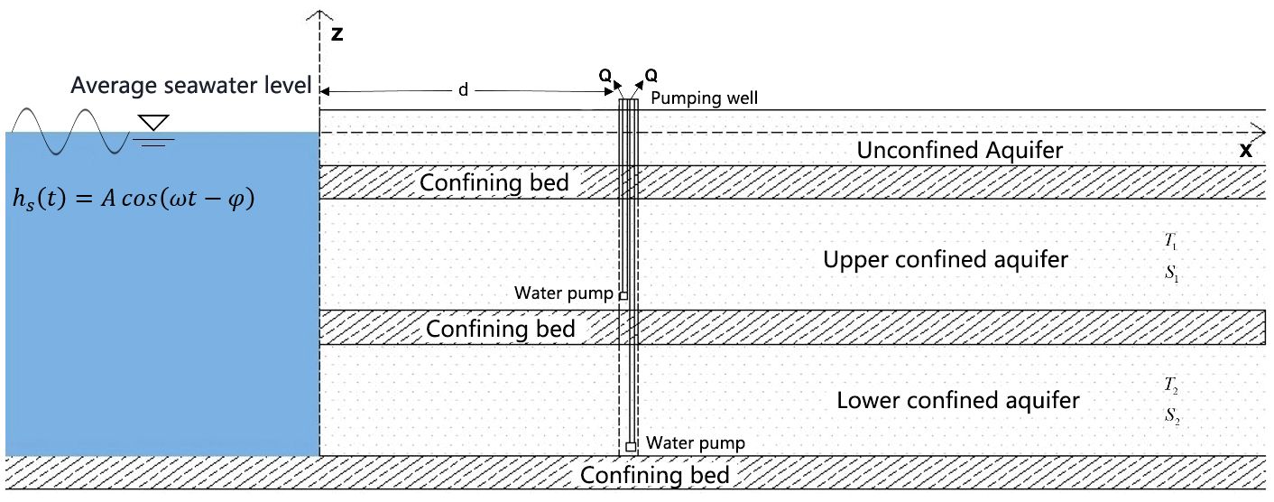
Figure 1 Schematic of pumping well in a multi-layered confined aquifer.
The x-axis is perpendicular to the coastline and points to the land in a positive direction. The intersection of the x-axis with the coastline is the coordinate origin. The y-axis is parallel to the coastline and coincides with the coastline. The z-axis is taken to be vertical and positive upward. Based on the above assumptions, the governing equations and boundary conditions of groundwater flow in the upper confined aquifer are expressed as the following equations:
where and T1 represent the hydraulic head [L], storage coefficient [−], and transmissivity [L2T−1] of the upper confined aquifer; is the hydraulic head of sea tide [L] at the time t [T]; A, represent the tidal amplitude [L], the tidal angular velocity [T−1], and the initial phase shift [−].
Ignoring the well storage effect of the pumping well, Darcy’s law is applied, and the boundary conditions on the wall of well can be written as
where Q is the pumping rate of the well [L3T−1], d is the distance [L] between the center of the well and the coastline, and r1 is the horizontal distance [L] between any point in the aquifer and the pumping well.
The governing equations and boundary conditions of the initial head in the aquifer influenced by the tide before pumping can be expressed as follows:
where H0 is the initial groundwater head [L] of the upper confined aquifer under the influence of tide before pumping.
The lower confined aquifer is similar to the upper confined aquifer, therefore, the description of its governing equations and boundary conditions is ignored here.
The solution of the mathematical models (Equations 5–7) is the analytical solution of groundwater level fluctuation in a confined aquifer given by Jacob (1950), which is under the boundary condition that the sea tide is a cosine function, namely, the initial condition of the mathematical model for the aquifer system can be expressed as follows:
where , which is an intermediate parameter. Therefore, one can have
In the traditional pumping test, the variation of hydraulic head is expressed by the drawdown, because the initial hydraulic head is a constant. However, the initial hydraulic head is not a constant under the effect of tide; therefore, H1 is used to describe the variation of hydraulic head as shown in Equation 9. As the coastline is the recharge boundary of the aquifer system, according to the theory of image method, there is an imaginary injection well with a flow rate of Q at the symmetrical position -d relative to the pumping well.
According to the formula of well flow and superposition principle in the confined aquifer without leakage recharge, the analytical solution of Equations 1–3, 4a, 4b can be obtained as follows (detailed derivation process is shown in Appendix A):
where
where W(u) is a well function, u1 and u2 are the intermediate parameters, the expression of r1 is shown in Equation 4b, and r2 is the horizontal distance between any point in the aquifer and the fictitious injection well [L].
The groundwater flow governing equations, boundary conditions, and initial conditions in the lower confined aquifer are consistent with those in the upper confined aquifer. Therefore, the analytical solution of the equations can be directly obtained as follows:
where are the intermediate parameters; the expressions of r1 and r2 are shown in Equations 4b, 10d; H2, S2 and T2 represent the hydraulic head [L], storage coefficient [−], and transmissivity [] of the lower confined aquifer.
In the coastal aquifer system without considering the leakage, the analytical solution of groundwater level fluctuation affected by tide is given by Jacob (1950), which is the analytical solution in a confined aquifer under the condition that the tide is a single cosine function (Hantush and Jacob, 1955).
When the pumping well is not considered or the pumping rate Q is equal to zero, the groundwater level fluctuation in the upper and lower confined aquifers satisfies the mathematical models (5) to (7). The solution of groundwater level fluctuation in the upper and lower confined aquifers is proposed by Jacob (1950). Namely Equation 12,
When the tidal effect is not considered or A = 0, the analytical solution of groundwater level fluctuation in the upper confined aquifer is written as follows:
where the expressions of W(u), u1, and u2 are shown in Equations 10b, c.
The analytical solution of groundwater level fluctuation in the lower confined aquifer is
where the expressions of W(u), are shown in Equations 10b, 11b.
When the tidal effect is not considered or A = 0, according to the principle of image method, Equations 13, 14 can be obtained, because the sea is the recharge boundary of the aquifer system. The Theis well function W(u) and its related properties and assumptions have been studied and analyzed in detail (Fetter, 1994); therefore, it is not described here.
Based on the above model, consider a coastal multi-layered aquifer system consisting of the unconfined aquifer and N-layered confined aquifers from top to bottom (Figure 2). There is an aquiclude between each two confined layers, and other assumptions are consistent with those of the above basic model. Based on the above assumptions, the governing equation and boundary conditions of groundwater flow in the Nth confined aquifer are as follows:
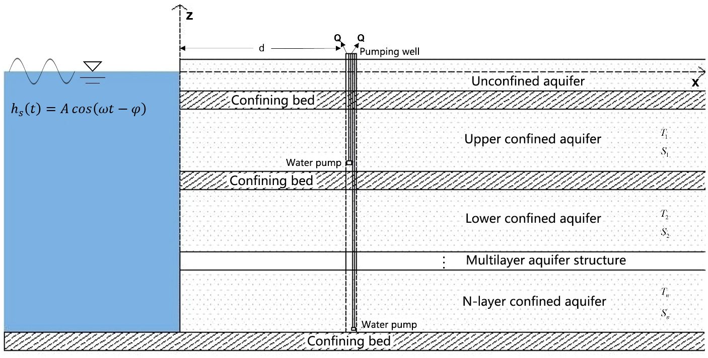
Figure 2 Schematic of pumping well in a N-layered confined aquifer.
where and represent the hydraulic head [L], storage coefficient [−], and transmissivity [] of the Nth confined aquifer.
The well storage effect of the pumping well is ignored, and Darcy’s law is applied. The boundary condition on the wall of well can be written as
The governing equation and boundary conditions of initial head in the Nth confined aquifer under the tidal influence before pumping can be expressed as follows:
where is the initial groundwater head [L] of the Nth confined aquifer under the influence of tide before pumping.
The boundary conditions and initial conditions of groundwater head in the Nth confined aquifer are consistent with those of the upper confined aquifer; therefore, the analytical solution of the equations can be obtained directly
where
For the groundwater fluctuation in the coastal N-layered confined aquifer system under the effects of tide and pumping, the Equations 15–23 can be used to solve it.
From the analytical solutions (10) and (11), it can be seen that the fluctuation of groundwater level under the effects of tide and well pumping is influenced by various parameters. It mainly includes parameters, which are tidal amplitude , initial phase shift , tidal angular velocity [], the distance between the well center and coastline d [L], the pumping rate of well Q [], storage coefficient S [−], and transmissivity T []. The impact of the main parameters in the analytical solution is discussed. The values of parameters for different cases are listed in Table 1.
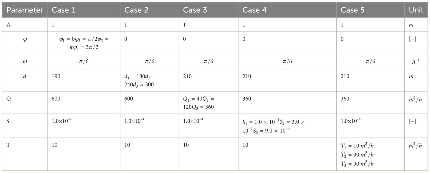
Table 1 Values of parameters for different cases.
Figure 3 shows how the groundwater head in the observation well located at varies with time when the initial phase shift = , , , and Table 1). From Figure 3 one can see that the groundwater head in the observation well decreases dramatically during the initial pumping stage and then tends to be stabilized gradually with time. There is a significant difference in the initial drawdown corresponding to different initial phases during the early stage of pumping, based on the groundwater head variation from 0 h to 15 h. It indicates that the initial phase of tide affects the initial drawdown in the observation well during the pumping. The primary justification behind this is the direct correlation between tide phase and the establishment of the groundwater level during pumping operations. The groundwater head fluctuations corresponding to different initial phases exhibit a significant lag relationship, namely, the phase difference. Therefore, the observed data of groundwater head during the long-term pumping should be used to estimate the hydrogeological parameters. Otherwise, there may be significant errors if one uses the data of groundwater head fluctuation during the early pumping.
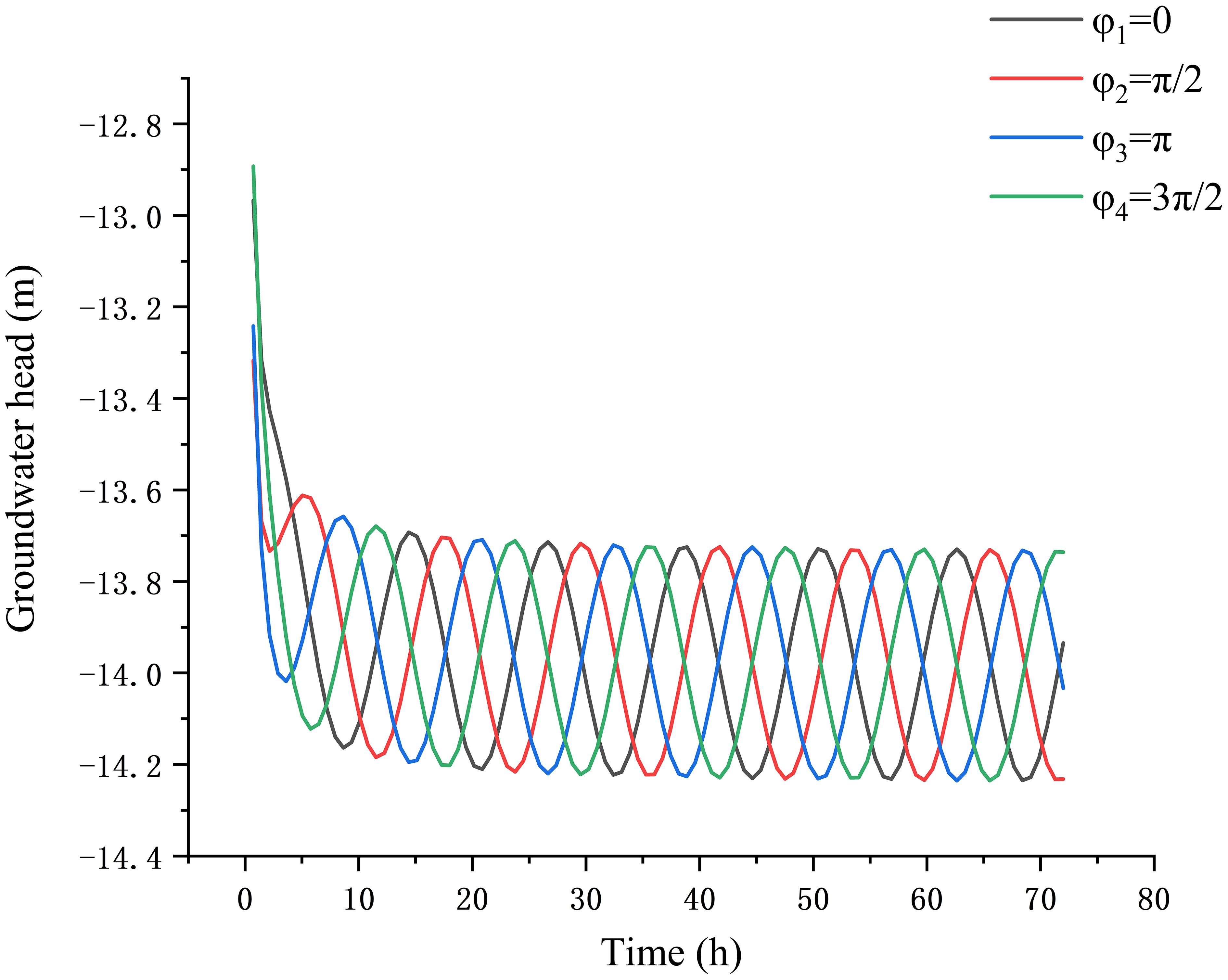
Figure 3 Changes of the groundwater head with time in the observation well located at (x0, y0) = (200 m, 0 m) during pumping for different values of the initial phase shifts.
Figure 4 shows the variation of groundwater head with time in the observed well at the location x = 200 m when d = , , respectively (Table 1). From Figure 4, one can see that the groundwater head in the observed well decreases rapidly within the initial 7 h of pumping. Then, it decreases gradually and stabilizes with time. The fluctuation of groundwater head in the aquifer exhibits periodic fluctuations, which is similar to tide. By comparing the three curves, it can be seen that the periodic fluctuation of groundwater head in the aquifer exhibits a lag phenomenon, as the distance from the pumping well to the coastline increases. The study further affirms that the influence of tidal fluctuations on groundwater levels decreases gradually from the coastal region to inland.
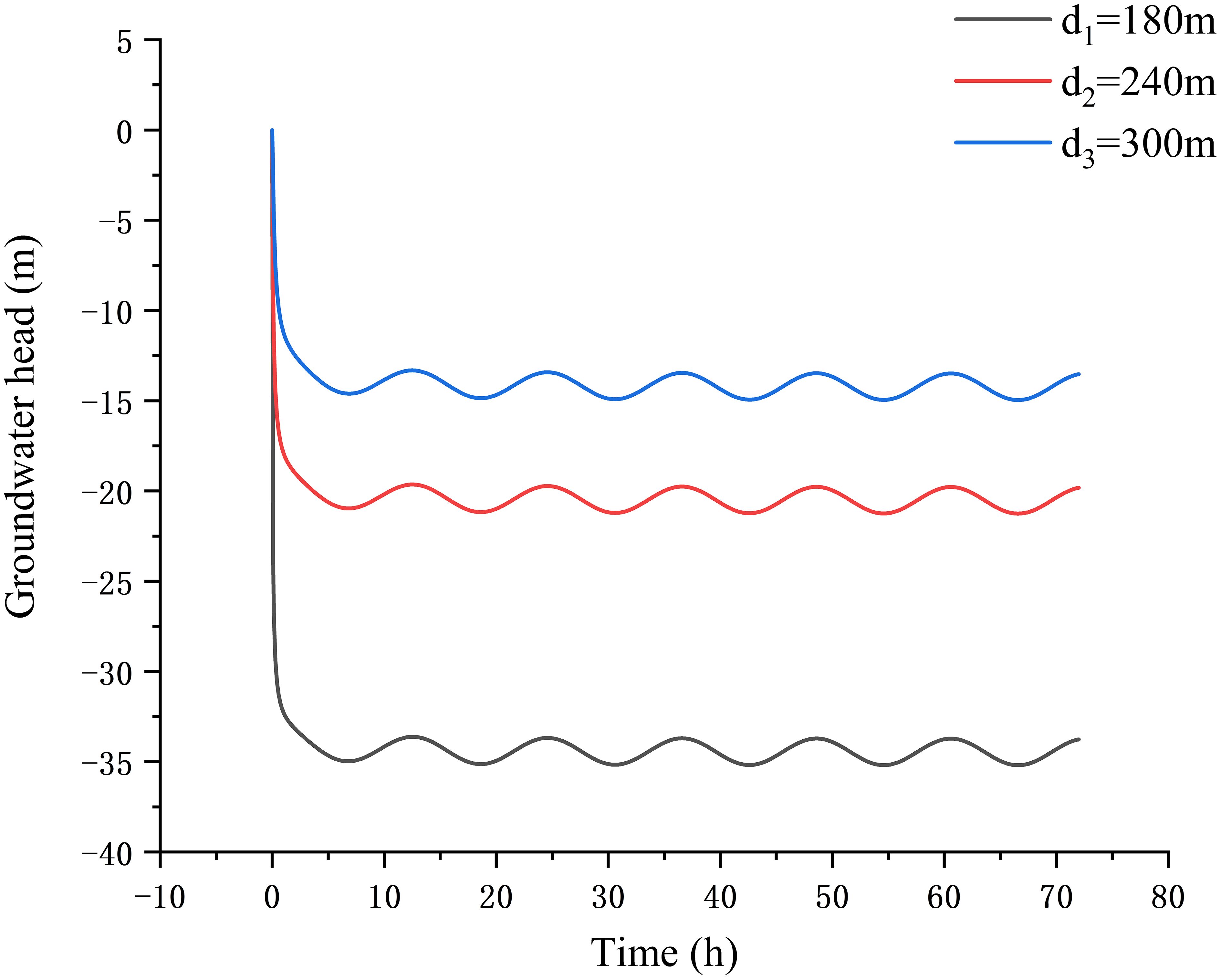
Figure 4 Changes of the groundwater head with time in an observed well located at x = 200 m during pumping for different values of the distance between the center of well and coastline.
Figure 5 shows the effects of pumping rate on the groundwater head fluctuation in the observed well at the location x = 290 m of the confined aquifer (Table 1). When the pumping rate is , the groundwater head in the observed well drops about 2 m and then reaches a quasi–steady state. When the pumping rate is , the groundwater head in the observed well drops about 7 m before reaching stability. It can be inferred that the pumping rate has a significant impact on the groundwater head in the observed well, and the high pumping flow rate causes an increase in the drawdown of the groundwater head. In the early stages of pumping, the groundwater head drops sharply due to the effect of pumping well. As the time increases, the groundwater head decreases rapidly in a short period of time, and, then, the decline rate decreases gradually. After 9 h, it can be seen that the fluctuation curve of the groundwater head shows the first obvious trough, and the groundwater head in the well stabilizes gradually, which presents a tidal fluctuation curve. By comparing the three curves, it can be found that as the pumping rate increases, the time for the groundwater level to reach a stable rate of decline increases. The aforementioned phenomenon is perceptible through the alteration of groundwater levels, which demonstrate that, as the amount of extraction increases, the difficulty in achieving and maintaining equilibrium also escalates.
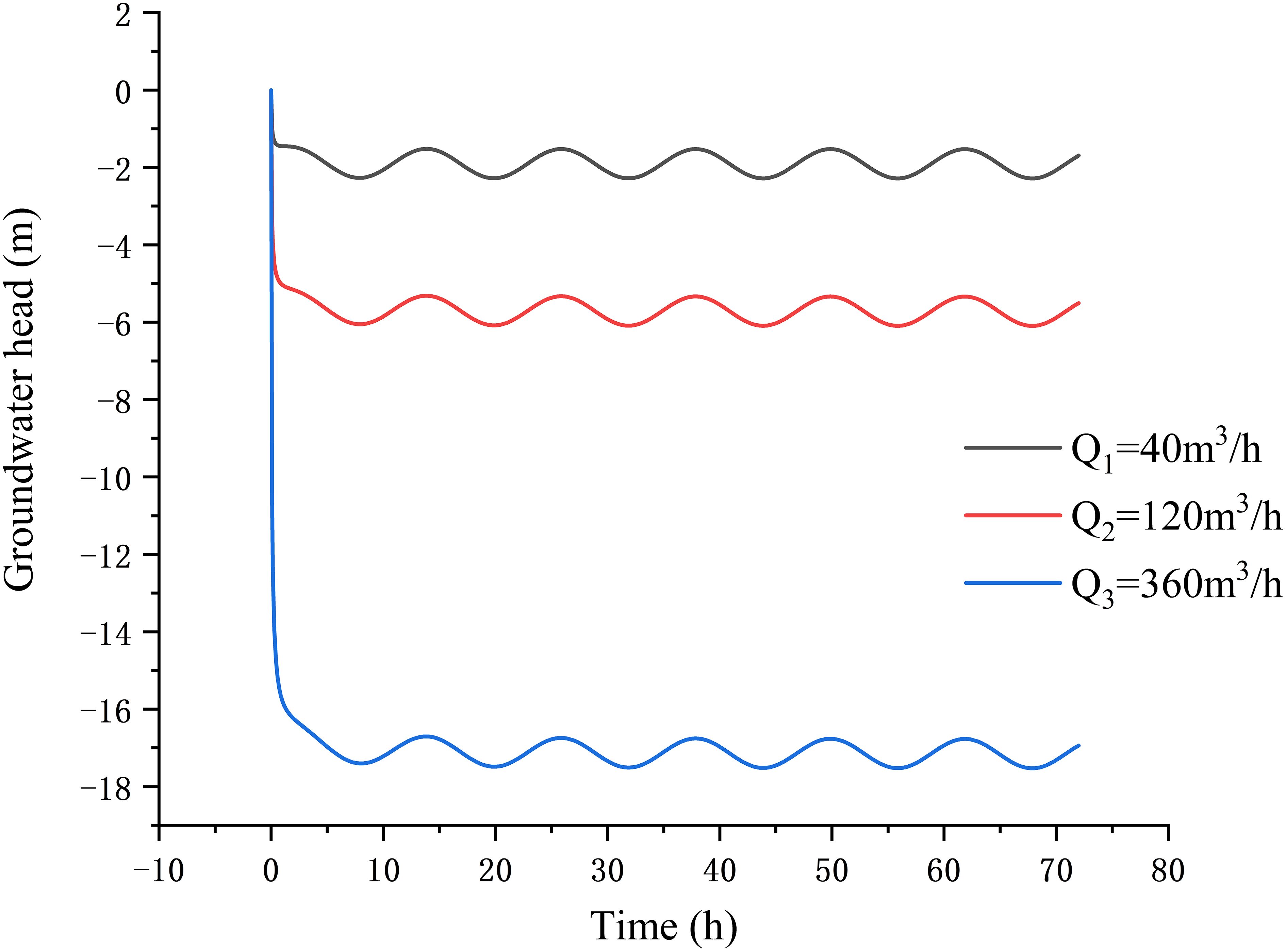
Figure 5 Variation of the groundwater head fluctuation in the observed well at the location x = 290 m of the confined aquifer for different values of pumping rate.
Figure 6 shows how the groundwater head in the observation well located at x = 190 m changes with time for different values of storage coefficient (Table 1). From Figure 6, one can see that the groundwater head decreases gradually with time for different values of storage coefficient. The groundwater head tends to be stabilized at the time of 8 h, when the storage coefficient is . The groundwater head gets a quasi–steady state at the time of 14 h, when the storage coefficient is . However, the decreasing trend of groundwater head after reaching stability is more significant. It indicates that the water level decrease caused by the pumping becomes slowly, as the storage coefficient increases. The groundwater level fluctuation tends to be stabilized and shows a significant cosine fluctuation, when the storage coefficient is . However, when the storage coefficient is , it can be found that the amplitude of groundwater level fluctuation is significantly weaker than that of the water storage coefficient (). At the same time, the fluctuation of groundwater level is almost invisible, when the storage coefficient is . It can be inferred that the storage coefficient affects the groundwater head significantly. As the storage coefficient increases, the fluctuation of groundwater level in the aquifer is less affected by the tidal fluctuations and shows a significant lag phenomenon.
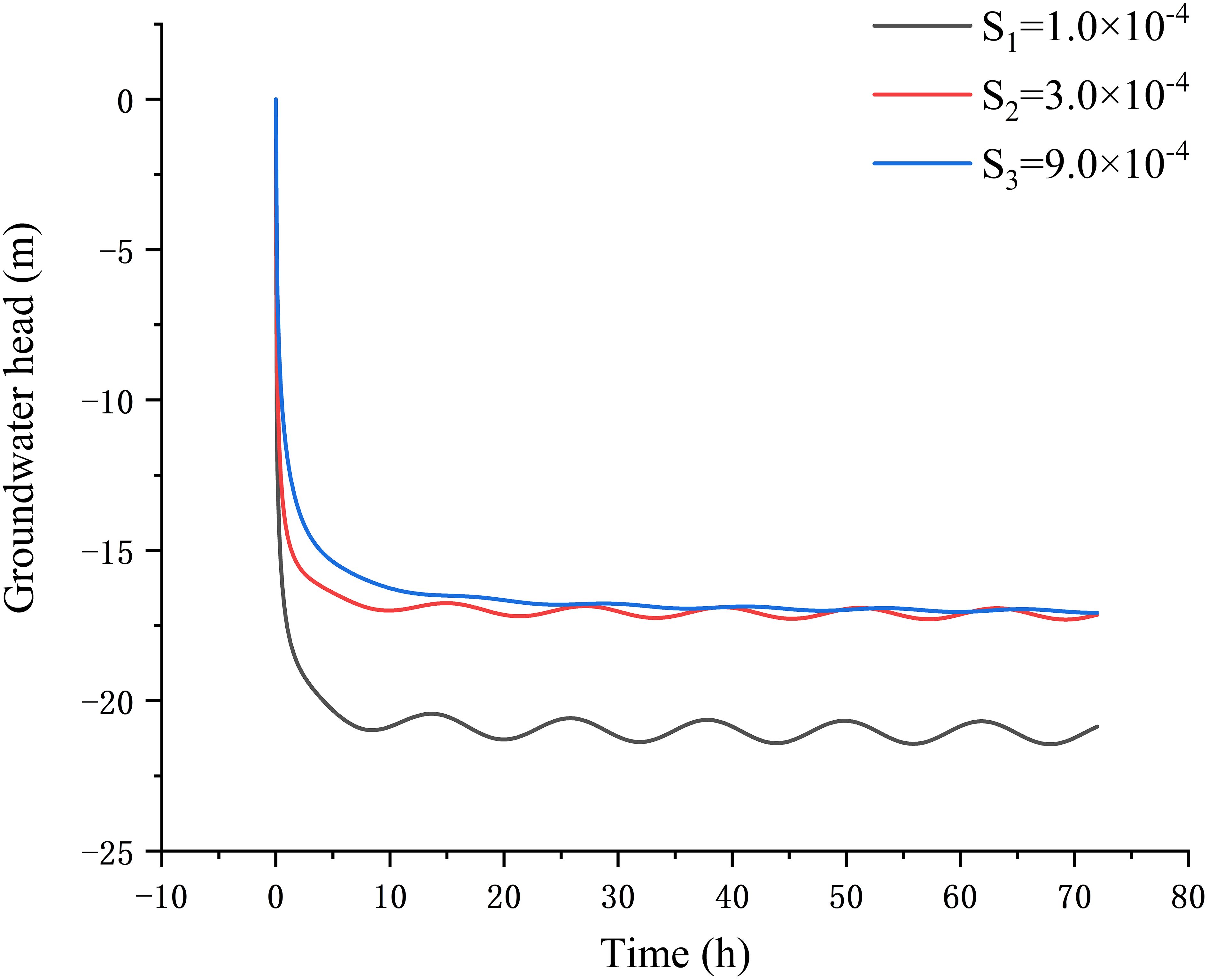
Figure 6 Variation of the groundwater head fluctuation in the observed well at the location x = 190 m of the confined aquifer for different values of storage coefficient.
Figure 7 shows how the groundwater head in the observation well located at x = 190 m changes with time for different values of transmissivity (Table 1). From Figure 7, one can see that the first time of a trough occurs in the groundwater head fluctuation curve is at 9 h, when the transmissivity is . However, the first obvious trough appears at 7 h when the transmissivity is . It indicates that the drawdown of groundwater head in the aquifer decreases as the transmissivity increases, and the periodic fluctuation of groundwater head shows a lag phenomenon. Comparing the three curves, it can be found that, when the values of transmissivity are , the amplitude of periodic fluctuation is 0.5 m, 1 m, and 1.2 m, respectively. It indicates that the periodic fluctuation of groundwater head in the aquifer is affected by tides, as the transmissivity increases. The transmissivity of the confined aquifer reflects the sensitivity of the groundwater level to hydrodynamic factors such as pumping and tides within the aquifer.
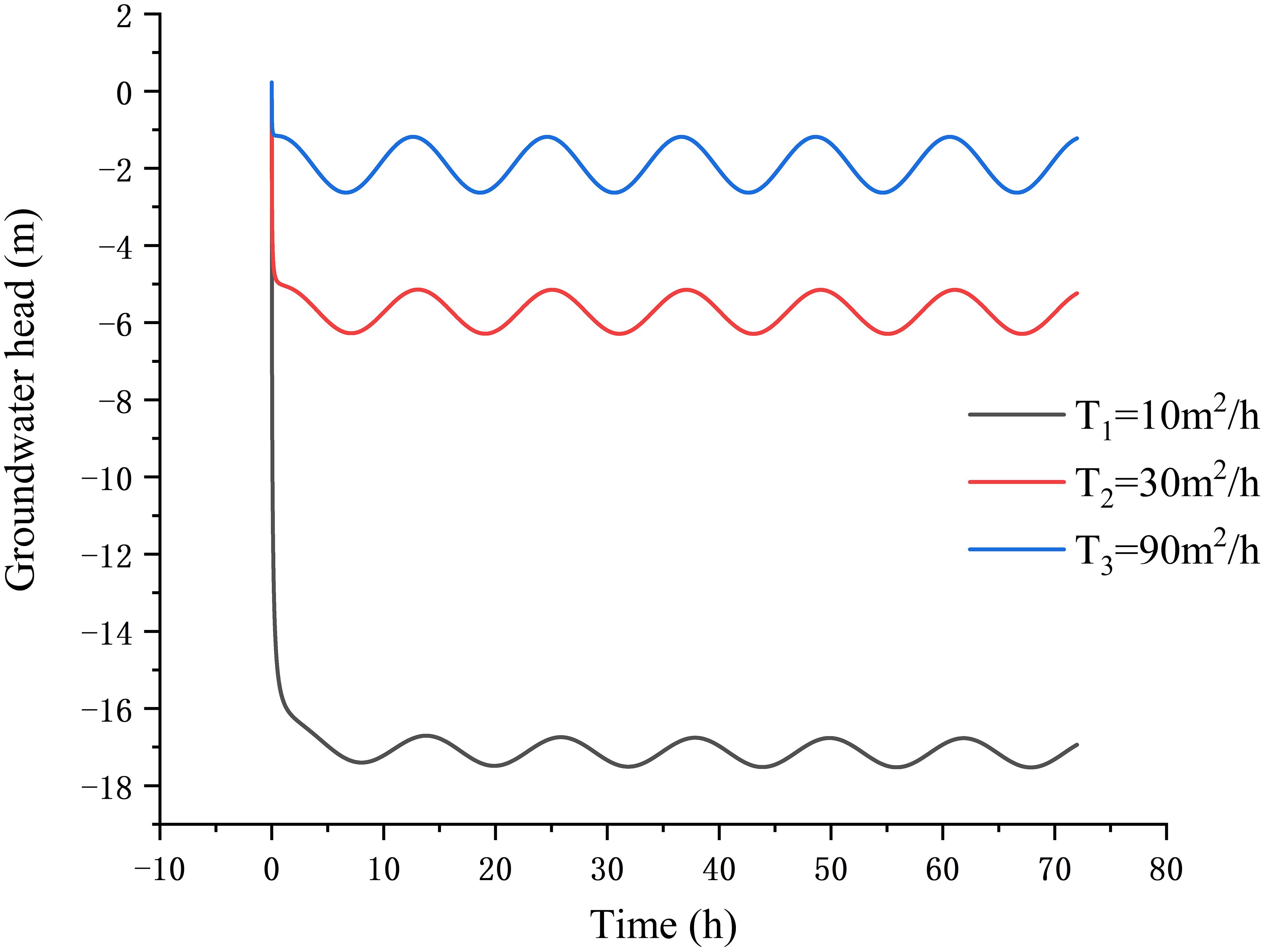
Figure 7 Variation of the groundwater head fluctuation in the observed well at the location x = 190 m of the confined aquifer for different values of transmissivity.
Wang et al. (2014) also consider the analytical solutions of groundwater level fluctuations under tidal and pumping conditions, and it considers the leakage between the unconfined aquifer and confined aquifer. However, this study considers the analytical solutions of groundwater level fluctuations in multi-layer aquifer systems and neglects the leakage between layers. Wang et al. (2014) separately discussed the influence of factors such as tidal phase and pumping flow on water level fluctuations, and it was difficult to distinguish the tidal effect from the head drop caused by pumping when the pumping time is less than half a tidal cycle. Wang et al. (2014) discussed the parameters of the two factors separately but did not combine the tidal and pumping. In this study, the discussion focuses on the interaction between the tidal and pumping conditions and further studies the combined effect of tidal and pumping on groundwater level fluctuations.
The study area is located in Longkou City, Shandong Province, China, which is situated in the northwestern part of the Jiaodong Peninsula (between 120°13′ and 120°44′ E longitude and 37°27′ and 37°47′ N latitude; Figure 8). The total area of Longkou City is about 901 km2. The maximum distance from north to south of Longkou is 37.43 km, and the maximum distance from east to west is 46.08 km, with a coastline of up to 68.4 km. The terrain and landform of Longkou City include the mountains, hills, and plains. The mountains are mainly located in the southeast of Longkou City, whereas the hills are located in the north of the southern part of the mountains. The plain area has formed three different types of landform due to its different genesis, including the coastal plain, the alluvial plain of mountain valley, and the alluvial plain in front of mountains. The exposed strata on the surface area are the Quaternary of the Cenozoic era, which mainly compose of sand, clay, and gravel. The research area has a semi-humid climate with significant seasonal changes, which is greatly affected by the monsoon. The average annual precipitation is 585.5 mm, which supplies the groundwater. The rivers are seasonal rivers in Longkou City, including the Huangshui River, Yongwen River, Beimanan River, Longkou North River, and Balisha River. The flow trend of groundwater is influenced by the terrain, which discharges into the Laizhou Bay from south to north. Longkou City is located in the warm temperate zone, with obvious characteristics of semi-humid monsoon land climate. It is heavily influenced by the monsoon and has four distinct seasons. There is less precipitation in spring, and the climate is dry, with the south wind as the main one; there is more rainfall in summer, with high and humid temperatures and more rainy weather; in autumn, the climate is dry and cool, with less rainfall; in winter, the temperature is low and the climate is cold, with the north wind as the main one. The average temperature for many years is 12.2°C, the maximum temperature is 38.3°C, the minimum temperature is −21.3°C, and the average evaporation for many years is 1479 mm. The average annual precipitation is 585.5 mm. Rainfall fluctuates greatly between years. There are significant differences in precipitation between seasons and regions. Rainfall in a year is most concentrated in July, August, and September. With the development of agriculture and industry, the demand for water such as farmland irrigation has increased, leading to high-intensity and unreasonable exploitation of groundwater in the area. As a result, the groundwater level in the coastal aquifer declines continuously in this area. In recent years, the problem of seawater intrusion in the region has been very serious. The measures were taken to prevent the seawater intrusion, and the area of seawater intrusion has gradually decreased.
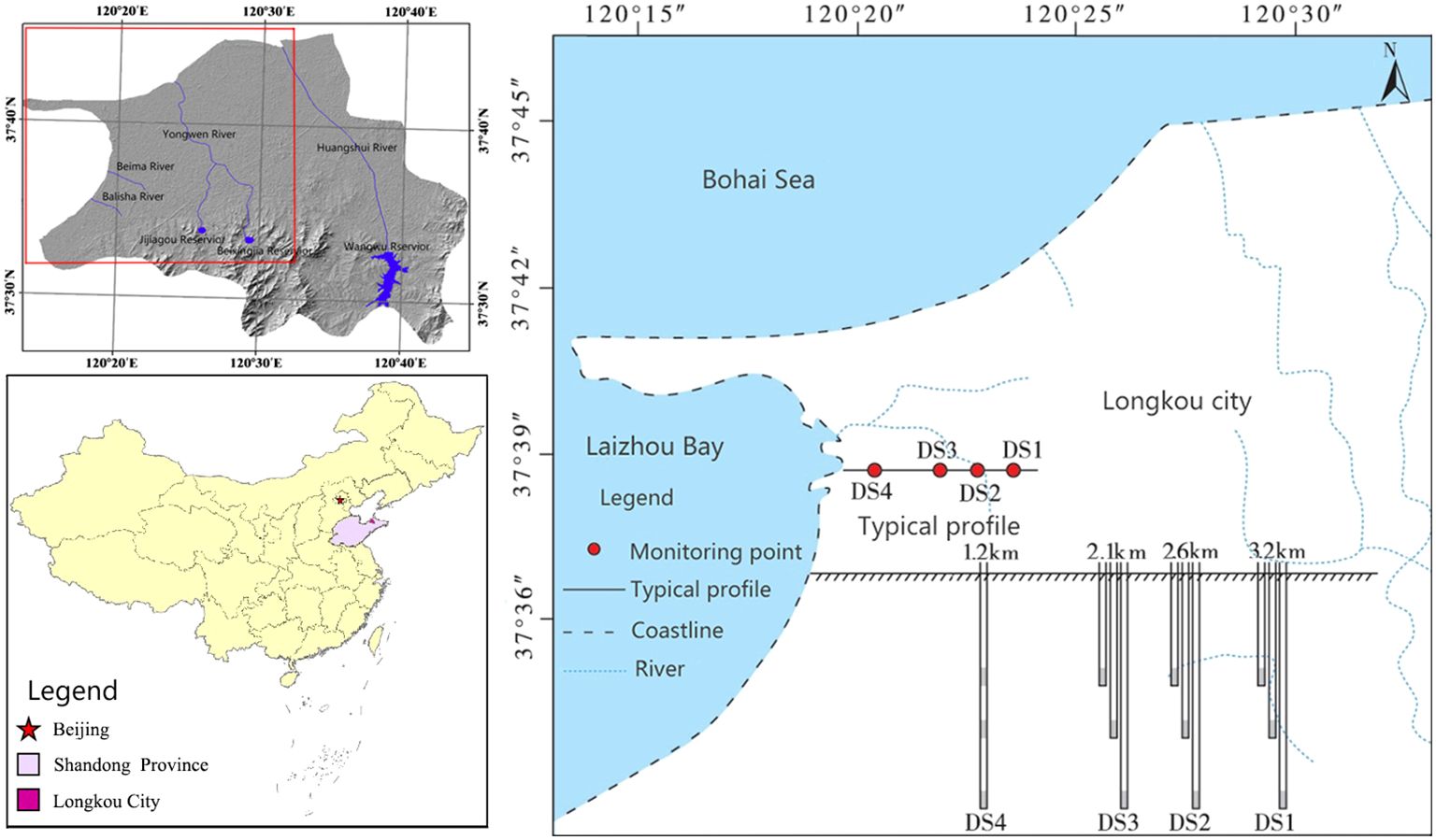
Figure 8 Distribution of monitoring wells in the seawater intrusion zone in Longkou City.
According to the drilling data, the coastal aquifer system of Longkou western coast is composed of three permeable layers and two aquicludes between them. The three permeable layers include an unconfined aquifer, an upper confined aquifer, and a lower confined aquifer, as illustrated in Figure 9. The distance of four groups of boreholes from the coastline is 1.2 km, 2.1 km, 2.6 km, and 3.2 km sequentially, and each group of boreholes is distributed in three different aquifers (Dai et al., 2020). The geologic information of the coastal aquifer system is described from up to down sequence. Coarse and medium sand in the unconfined aquifer, sand and gravel in the upper confined aquifer, and coarse sand and gravel in the lower confined aquifer. The average thickness of the unconfined aquifer is about 3.30 m, the upper confined aquifer is about 4.00 m, and the lower confined aquifer is also about 4.00 m. Based on slug tests conducted at different depths of boreholes, the hydraulic conductivities of different aquifers were obtained, and they were about 2.93 m/h for the unconfined aquifer, from 1.47 m/h to 3.58 m/h for the upper confined aquifer, and from 1.20 m/h to 5.22 m/h for the lower confined aquifer. The groundwater head and water quality in each borehole were monitored.
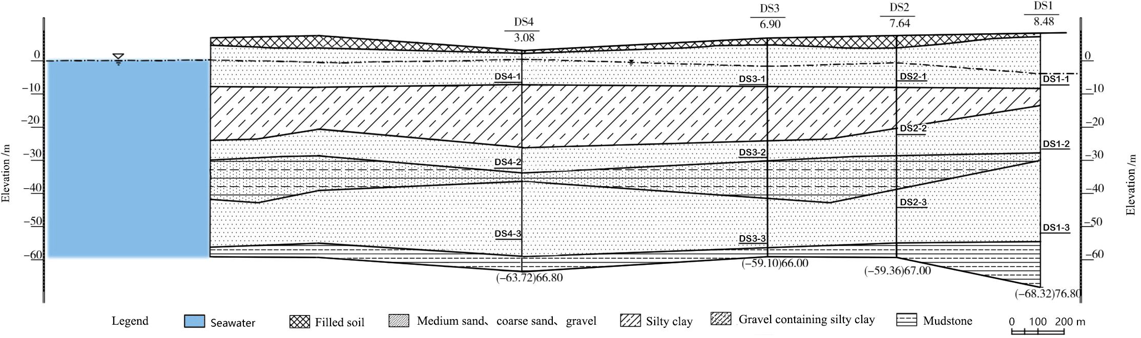
Figure 9 Generalizing the field test stratigraphic profile.
In order to verify the applicability of the analytical solution, the parameters in the analytical solution are assigned with reference to the actual situation (Table 2). The thickness and storage coefficient of the aquifer were determined by the oscillation test conducted by Dai et al. in the groundwater stratification monitoring well in the Longkou seawater intrusion area (Dai et al., 2020). The tidal amplitude , initial phase shift and tidal angular velocity of tidal fluctuations are derived from the tidal prediction table of Longkou City when the monitoring well is working. The variation of the water level in the upper and lower confined aquifers are calculated within 60 h (2.5 cycles of sea tide). The value of the pumping rate of well is 400 m3/h as shown in Table 2, and the pumping period is 60 h. The water level data in the four monitoring wells—DS3–2, DS4–2, DS3–3, and DS4–3—were selected to fit the analytical solution. Therefore, the inverse problem can be used to establish the corresponding solution method.
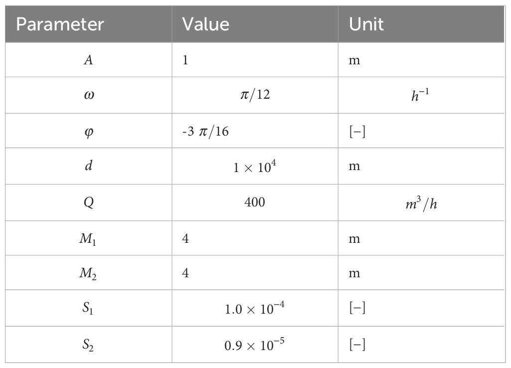
Table 2 Values of the parameters.
Let
According to Equations 8, 10a–d, 24, one can obtain that
when approaches zero, the change rate in groundwater head fluctuation of the upper confined aquifer is zero. It means that is equal to zero, when reaches its extreme value.
Based on the measured curve of H relative to t, the extreme value of the curve can be derived. Then, according to the values of parameters in Table 2, the hydraulic conductivity of the upper confined aquifer can be obtained based on Equation 25. The groundwater level within 60 h (2.5 tidal cycles) in the monitoring well DS2–2 was selected. The average value −1.78 m of it was taken as the initial head . Figure 10 shows the changes of the observed with time in the well DS2–2. From Figure 10 one can see that the extreme values of are 8 h, 31 h, and 45 h. Therefore, the values of the hydraulic conductivity of the upper confined aquifer are 3.07 m/h, 3.36 m/h, and 3.77 m/h, respectively, based on the Table 2 and Equation 25. The data collation is shown in DS2–2 of Table 3. The average value of in the upper confined aquifer is 3.4 m/h, which is in the range from 1.47 m/h to 3.58 m/h as shown above. The calculated groundwater head based on the analytical solution (10) is shown in Figure 10, according to the hydraulic conductivity and other parameters listed in Table 2. The mean square error () between the observed groundwater head and the predicted value calculated by the analytical solution (10) can be written as follows:
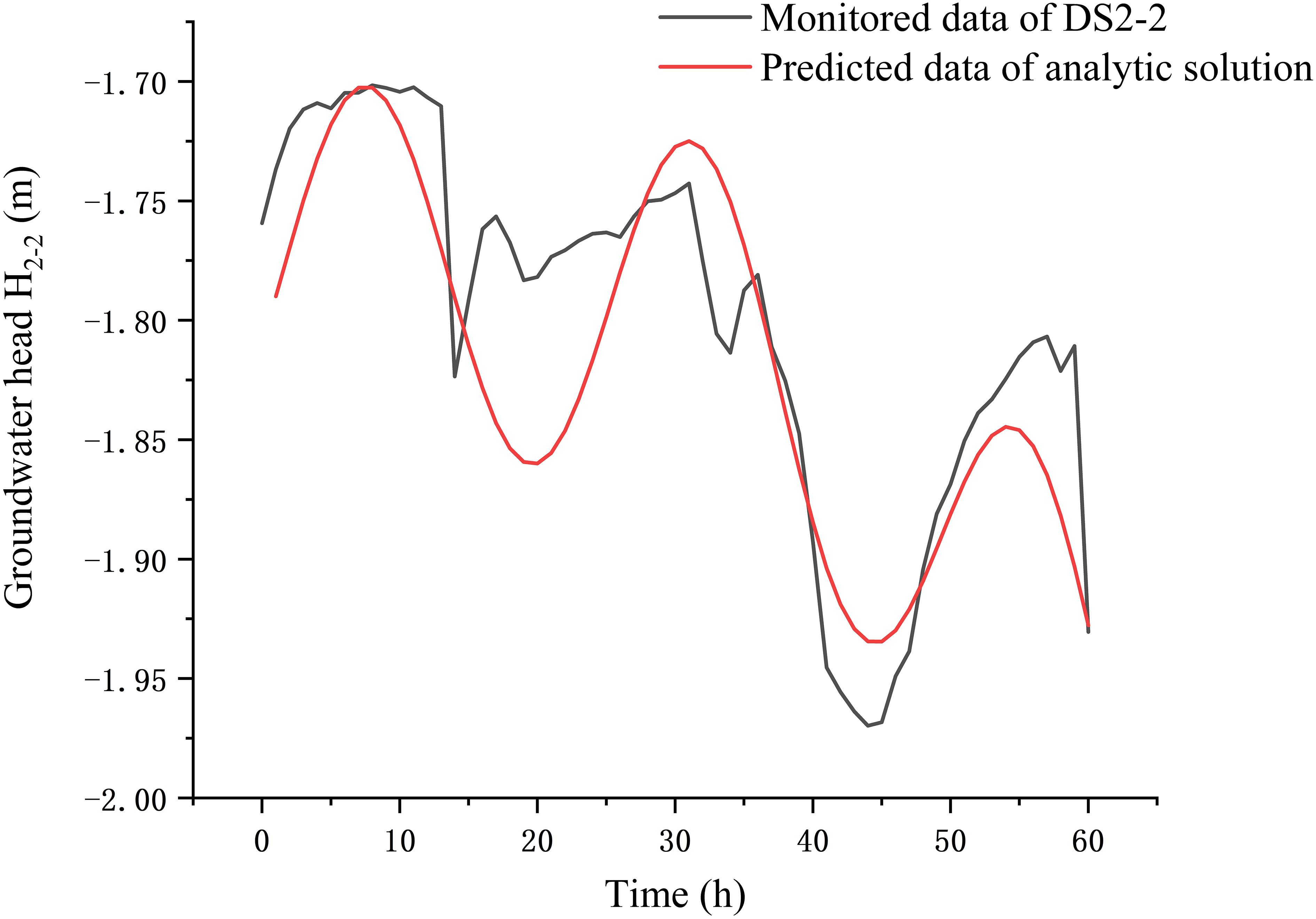
Figure 10 Comparison of the results of the analytical solution simulation with the monitoring data of well DS2–2.
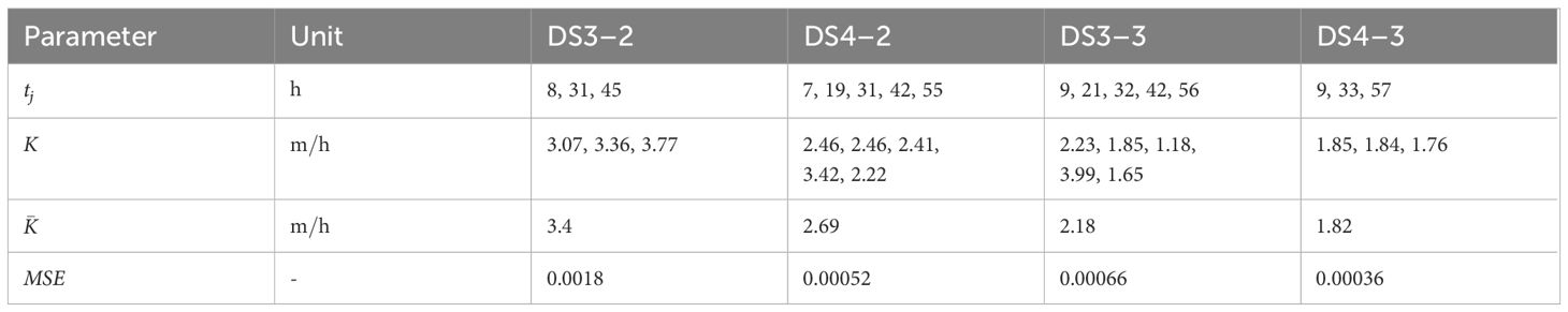
Table 3 The data collation of parameter estimation.
where is the observed groundwater head and is the predicted value calculated by the analytical solution (10). Therefore, is 0.0018 based on Figure 10 and Equation 26.
The observed groundwater level within 60 h (2.5 sea tide cycles) in the monitoring well DS3–2 was chosen, and the average value of it was taken as the initial head, namely, is equal to −4.83 m. Figure 11 shows the variation of the observed with time in the well DS3–2. From Figure 11, one can see that the extreme values of are 7 h, 19 h, 31 h, 42 h, and 55 h. Therefore, the values of the hydraulic conductivity in the upper confined aquifer are 2.46 , 2.46 , 2.41 , 3.42 , and 2.22 , respectively, based on Table 2 and Equation 25. The data collation is shown in DS3–2 of Table 3. The average value of the hydraulic conductivity in the upper confined aquifer is , which is in the range between 1.47 m/h and 3.58 m/h. According to the average value of and the other parameters assigned in Table 2, the calculated value based on the analytical solution (10) is also plotted and shown in Figure 11. The mean square error between the observed groundwater level and the predicted value in the monitoring well DS3–2 is 0.00052.

Figure 11 Comparison of the results of the analytical solution simulation with the monitoring data of well DS3–2.
In fact, the fluctuation of seawater level is influenced by the spring-neap tides. Moreover, the layers between each two aquifers are relative aquicludes, and there maybe leakage recharge between layers. Therefore, the analytical solution under ideal conditions could not fully match the fluctuation of the groundwater level. Nevertheless, the fitted results of the analytical solution capture the main characteristics of the groundwater level affected by the tidal fluctuation and groundwater pumping as shown in Figures 10, 11. Based on the fitted curves of groundwater head in wells DS2–2 and DS3–2, one can observe a marked fluctuation in groundwater head in correlation with the tide, revealing a progressive decrease with increasing elapsed time. At the same time, the amplitude of groundwater level shows a decreasing trend. Comparing Figures 10, 11, it can be found that the decreasing trend of groundwater level in well DS2–2 is more obvious than that in well DS3–2. The reason is that the distance from the pumping well for well DS2–2 is closer than that of DS3–2. It indicates that the decreasing rate of groundwater head increases as the distance of observed well from the pumping well decreases.
Similarly, let
According to Equations 8, 10a–d, 27, one can obtain
when approaches zero, the change rate of groundwater head in the lower confined aquifer is 0. The value of is equal to zero, when reaches its extreme value.
The observed groundwater level in the monitoring well DS3–3 within 60 h (2.5 sea tide cycles) was selected, and the average value was taken as the initial head . Figure 12 reports the variations of the observed groundwater level with time in well DS3–3. It can be found that the extreme values of are 9 h, 21 h, 32 h, 42 h, and 56 h. Thus, the values of hydraulic conductivity of the lower confined aquifer are 2.23 m/h, 1.85 m/h, 1.18 m/h, 3.99 m/h, and 1.65 m/h, respectively, based on the parameters in Table 2 and Equation 28. The data collation is shown in DS3–3 of Table 3. The average value of hydraulic conductivity of the lower confined aquifer is , which is in the range between as shown above. The calculated values of based on the analytical solution (11) are also plotted in Figure 12, according to the hydraulic conductivity and the other parameters listed in Table 2. The mean square error between the observed values of the groundwater level and the predicted ones in the monitoring well DS3–2 is 0.00066.
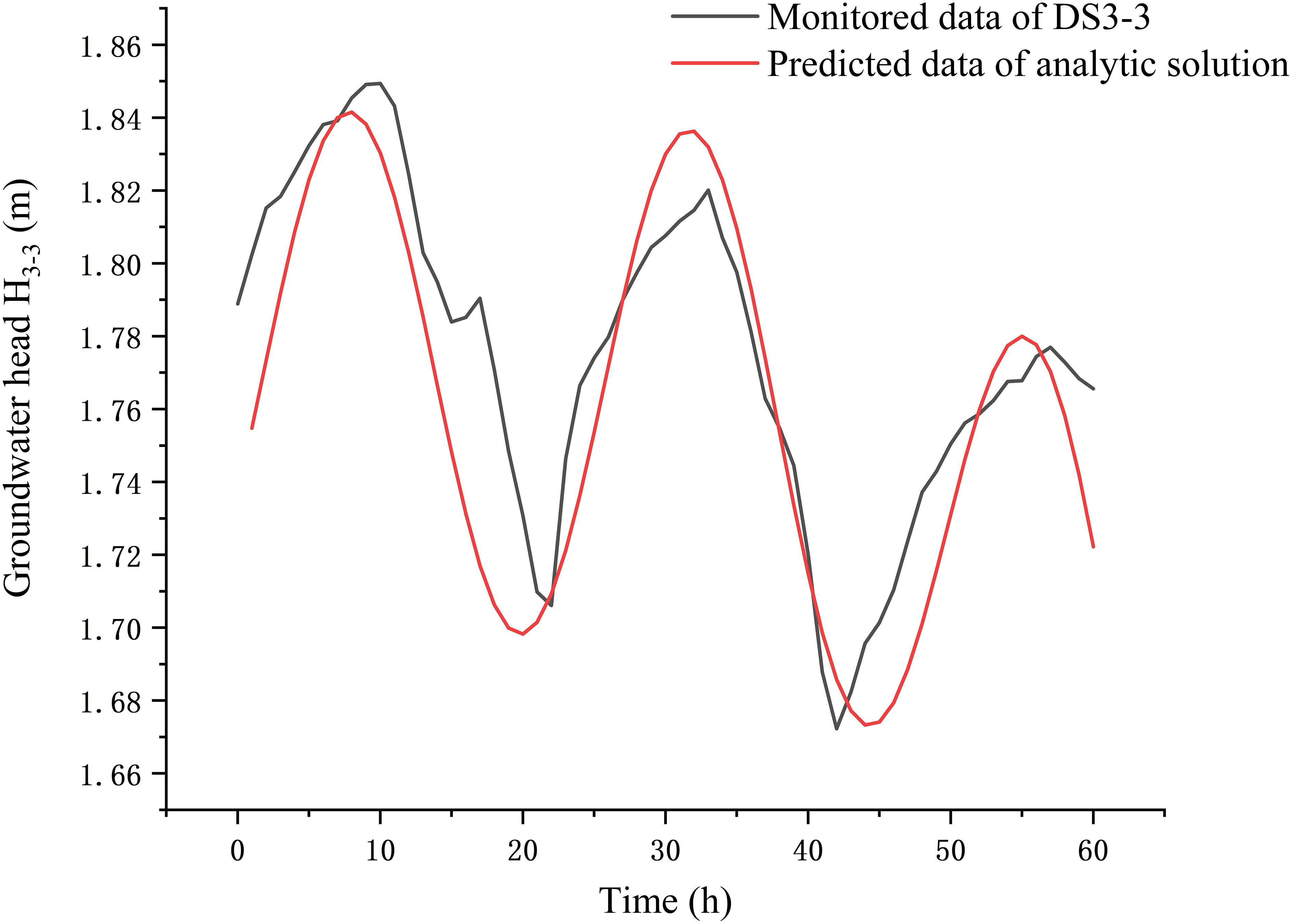
Figure 12 Comparison of the results of the analytical solution simulation with the monitoring data of well DS3–3.
The observed groundwater level in the monitoring well DS4–3 within 60 h (2.5 sea tide cycles) was selected, and the average value of groundwater head was . Figure 13 shows the variations of the observed groundwater level with time in well DS3–3. The observed extreme values of are 9 h, 33 h, and 57 h. The values of the hydraulic conductivity of the lower confined aquifer are 1.85 , 1.84 , and 1.76 , respectively, based on the parameters listed in Table 2 and Equation 28. The data collation is shown in DS4–2 of Table 3. The average value of the hydraulic conductivity of the lower confined aquifer is , which is in the range between as shown above. The calculated groundwater level based on the analytical solution (11) is also reported in Figure 13, according to the hydraulic conductivity and other parameters listed in Table 2. The mean square error between the observed values of groundwater head and the predicted ones in the monitoring well DS4–3 is 0.00036.
Figure 13 Comparison of the results of the analytical solution simulation with the monitoring data of well DS4–3.
Figures 12, 13 show the fitting curves between the measured groundwater level and the calculated one in the wells of the lower confined aquifer based on Equations 11a, b. In general, the calculated groundwater level in the lower confined aquifer fits well with the measured one. Similar to Figures 10–13 show that the groundwater level in the lower confined aquifer fluctuates with the tide, and the amplitude of it decreases gradually with groundwater pumping. At the same time, it can be observed that the decreasing trend of the groundwater level in well DS3–3 is more significant than that in well DS4–3, by comparing Figures 12, 13. It is mainly due to the fact that well DS3–3 is closer to the pumping well, which is influenced by the pumping significantly. The calculated groundwater level based on the analytical solution fits well with the observed one, which shows the main characteristics of groundwater fluctuation effected by the tide and groundwater pumping.
To sum up, the estimated values of the hydraulic conductivities in the upper and lower confined aquifers are within the range of the values obtained from the field experiments (Dai et al., 2020). The small error value of MSE for each case indicates a good fit between the calculated and observed groundwater head. It indicates that the method for calculating the hydraulic conductivity based on the analytical solutions (10) and (11) and Equations 25, 28 is reasonable and reliable.
This paper considered groundwater head fluctuation in the coastal multi-layered aquifer system caused by tide and groundwater exploitation. The multi-layered aquifer system is composed of an unconfined aquifer, an upper confined aquifer, and a lower confined aquifer from top to bottom. There is an aquiclude between each two aquifers. All the layers terminate at the coastline and extend infinitely toward the land. The new analytical solutions describing the groundwater head variation in the coastal multi-confined aquifer system are presented. Superposition principle and image methods are used for the derivation of the analytical solutions. Analytical solutions of different situations of without considering pumping, of without considering tidal effect, of N-layered confined aquifers are also discussed.
The fluctuation of groundwater head in the upper and lower confined aquifers under the effects of tide and well pumping is influenced by the main parameters, including the initial phase shift of tide, pumping rate of well, position of the pumping well, storage coefficient, and transmissivity. The initial phase shift of tide has a significant impact on groundwater head, controlling the initial groundwater head and the magnitude and rate of groundwater head decline before pumping. As the distance from the pumping well to the coastline increases, the periodic fluctuation of the groundwater head exhibits a lag phenomenon during the pumping. The pumping rate influences the groundwater head, and the higher pumping rate causes decrease of groundwater head dramatically. As the storage coefficient increases, the fluctuation of groundwater head in the aquifer is less affected by the tide and shows a significant lag phenomenon. However, as the transmissivity increases, the periodic fluctuation of groundwater head in the aquifer is affected by the tide.
Our solutions are applied to analyze the observed groundwater head fluctuation caused by the tide and pumping in the wells, which situated in the coastal zone of Longkou City, Shandong Province, China. The method for calculating hydraulic conductivities based on the analytical solutions (10) and (11) and Equations 25, 28 is reasonable and reliable. The estimated values of hydraulic conductivities in the upper and lower confined aquifers are within the range of the values obtained from the field experiments. The smaller error value of MSE for each case indicates a good fit between the calculated groundwater head and observed one. The fitted results of the analytical solutions capture the main characteristics of groundwater head fluctuation affected by the tide and groundwater pumping. The study of groundwater head fluctuation in the coastal multi-layer aquifer system is helpful to understand the mechanism of seawater intrusion under the influence of tide and groundwater pumping.
The analytical solutions appear in aquifer systems where aquifers are separated by aquicludes, but aquifers may also be separated by aquitards, so further consideration should be given to leakage between aquifers based on analytical solutions. New analytical solutions applicable to aquifer systems where aquifers are separated by aquitards should be discussed in the future. Simplified aquifer systems often struggle to accurately accommodate the intricacies of complex geologic formations. To more accurately represent the consequences of the apparent mismatch between the actual geological environment and the simplified aquifer model, it is often useful to employ numerical simulations to clarify potential differences between analytical and numerical results or to develop more complex analytical or semi-analytical approaches in the future.
The raw data supporting the conclusions of this article will be made available by the authors, without undue reservation.
QG: Writing – original draft. JL: Data curation, Investigation, Writing – original draft. XZ: Formal analysis, Writing – review & editing. YD: Investigation, Writing – review & editing.
The author(s) declare financial support was received for the research, authorship, and/or publication of this article. This work was supported by the National Natural Science Foundation of China (Grant No. 41772235).
The authors declare that the research was conducted in the absence of any commercial or financial relationships that could be construed as a potential conflict of interest.
All claims expressed in this article are solely those of the authors and do not necessarily represent those of their affiliated organizations, or those of the publisher, the editors and the reviewers. Any product that may be evaluated in this article, or claim that may be made by its manufacturer, is not guaranteed or endorsed by the publisher.
Ackerer P., Carrera J., Delay F. (2023). Identification of aquifer heterogeneity through inverse methods. Comptes Rendus Geosci. 355, 45–58. doi: 10.5802/crgeos.162
Bakker M. (2019). Analytic solutions for tidal propagation in multilayer coastal aquifers. Water Resour. Res. 55, 3452–3464. doi: 10.1029/2019WR024757
Bresciani E., Batelaan O., Banks E. W., Barnett S. R., Batlle-Aguilar J., Cook P. G., et al. (2015a). Assessment of Adelaide Plains Groundwater Resources: Summary Report (Adelaide, South Australia: Goyder Institute for Water Research Technical Report Series No. 15/31).
Bresciani E., Batelaan O., Banks E. W., Barnett S. R., Batlle-Aguilar J., Cook P. G., et al. (2015b). Assessment of Adelaide Plains Groundwater Resources: Appendices Part I – Field and Desktop Investigations (Adelaide, South Australia: Goyder Institute for Water Research Technical Report Series No. 15/32).
Cartwright N., Nielsen P., Li L. (2004). Experimental observations of watertable waves in an unconfined aquifer with a sloping boundary. Adv. Water Resour. 27, 991–1004. doi: 10.1016/j.advwatres.2004.08.006
Chapuis R. P., Belanger C., Chenaf D. (2006). Pumping test in a confined aquifer under tidal influence. Ground Water. 44, 300–305. doi: 10.1111/j.1745-6584.2005.00139.x
Chuang M. H., Yeh H. D. (2007). An analytical solution for the head distribution in a tidal leaky confined aquifer extending an infinite distance under the sea. Adv. Water Resour. 30 (3), 439–445. doi: 10.1016/j.advwatres.2006.05.011
Chuang M. H., Yeh H. D. (2011). A generalized solution for groundwater head fluctuation in a tidal leaky aquifer system. J. Earth Syst. Sci. 120, 1055–1066. doi: 10.1007/s12040-011-0128-8
Dai Y., Lin J., Guo Q., Sun X., Chen Y., Liu J. (2020). Experimental study on rapid evaluation of formation permeability in seawater intrusion area. J. Hydraulic Engineering. 10), 1234–1247. doi: 10.13243/j.cnki.slxb.20200108
Das K., Debnath P., Layek M. K., Sarkar S., Ghosal S., Mishra A. K., et al. (2022). Shallow and deep submarine groundwater discharge to a tropical sea: Implications to coastal hydrodynamics and aquifer vulnerability. J. Hydrol. 605, 127335. doi: 10.1016/j.jhydrol.2021.127335
Debnath P., Mukherjee A., Singh H. K., Mondal S. (2015). Delineating seasonal porewater displacement on a tidal Cat in the Bay of Bengal by thermal signature: Implications for submarine groundwater discharge. J. Hydrol. 29, 1185–1197. doi: 10.1016/j.jhydrol.2015.09.029
Guo Q., Huang J., Zhou Z., Wang J. (2019). Experiment and numerical simulation of seawater intrusion under the influences of tidal fluctuation and groundwater exploitation in coastal multilayered aquifers. Geofluids. 2019, UNSP 2316271. doi: 10.1155/2019/2316271
Guo Q., Li H., Boufadel M. C., Xia Y., Li G. (2007). Tide-induced groundwater head fluctuation in coastal multi-layered aquifer systems with a submarine outlet-capping. Adv. Water Resour. 30, 1746–1755. doi: 10.1016/j.advwatres.2007.01.003
Hantush M. S., Jacob C. E. (1955). Non-steady radial flow in an infinite leaky aquifer. Transactions Am. Geophysical Union 36, 95–100. doi: 10.1029/TR036i001p00095
Hsieh P. C., Hsu H. T., Liao C. B., Chiueh P. T. (2015). Groundwater response to tidal fluctuation and rainfall in a coastal aquifer. J. Hydrol. 521, 132–140. doi: 10.1016/j.jhydrol.2014.11.069
Huizer S., Karaoulis M., Oude Essink G., Bierkens M. (2017). Monitoring and simulation of salinity changes in response to tide and storm surges in a sandy coastal aquifer system. Water Resour. Res. 53, 6487–6509. doi: 10.1002/2016WR020339
Jacob C. E. (1950). “Flow of groundwater,” in Engineering Hydraulics. Ed. Rouse H. (John Wiley& Sons Inc, New York), 321–386.
Jasechko S., Perrone D., Seybold H., Fan Y., Kirchner J. W. (2020). Groundwater level observations in 250,000 coastal US wells reveal scope of potential seawater intrusion. Nat. Commun. 11, 1–9. doi: 10.1038/s41467-020-17038-2
Li G. M., Chen C. X. (1991). Determining the length of confined aquifer roof extending under the sea by the tidal method. J. Hydrol. 123, 97–104. doi: 10.1016/0022-1694(91)90071-O
Li H., Jiao J. J. (2001b). Tide-induced groundwater fluctuation in a coastal leaky confined aquifer system extending under the sea. Water Resour. Res. 37 (5), 1165–1171. doi: 10.1029/2000WR900296
Li H., Jiao J. J. (2003). Tide-induced seawater-groundwater circulation in a multi-layered coastal leaky aquifer system. J. Hydrol. 274 (1-4), 211–224. doi: 10.1016/S002-1694(02)00413-4
Li H. L., Jiao J. J. (2001a). Analytical studies of groundwater-head fluctuation in a coastal confined aquifer overlain by a leaky layer with storage. Adv. Water Resour. 24, 565–573. doi: 10.1016/S0309-1708(00)00074-9
Li M. W., Zhou Z. F., Huang H. L., Liao J. X. (2022). Estimation of hydraulic diffusivity of a confined limestone aquifer at the Xiluodu Dam. Geofluids. 2022, 8732415. doi: 10.1155/2022/8732415
Lu C., Xin P., Li L., Luo J. (2015). Steady state analytical solutions for pumping in a fully bounded rectangular aquifer. Water Resour. Res. 51, 8294–8302. doi: 10.1002/2015WR017019
Luo Z. Y., Kong J., Barry D. A. (2023). Watertable fluctuations in coastal unconfined aquifers with a sloping sea boundary: Vertical flow and dynamic effective porosity effects. Adv. Water Resour. 178, 104491. doi: 10.1016/j.advwatres.2023.104491
Marshall S. K., Cook P. G., Simmons C. T., Konikow L. F., Dogramaci S. (2022). An approach to include hydrogeologic barriers with unknown geometric properties in groundwater model inversions. Water Rsources Resour. 58, e2021WR031458. doi: 10.1029/2021WR031458
Noorabadi S., Nazemi A. H., Sadraddini A. A., Delirhasannia R. (2017). Laboratory investigation of water extraction effects on saltwater wedge displacement. Global J. Environ. Sci. Manage. 3 (1), 21–32. doi: 10.22034/gjesm.2017.03.01.003
Peters C. N., Kimsal C., Frederiks R. S., Paldor A., McQuiggan R., Michael H. A. (2022). Groundwater pumping causes salinization of coastal streams due to baseflow depletion: analytical framework and application to Savannah River,GA. J. Hydrol. 604, 127238. doi: 10.1016/j.jhydrol.2021.127238
Ratner-Narovlansky Y., Weinstein Y., Yechieli Y. (2020). Tidal fluctuations in a multiunit coastal aquifer. J. Hydrol. 580, 124222. doi: 10.1016/j.jhydrol.2019.124222
Ren H. L., Tao Y. Z., Lin F., Wei T. (2022). Analytical solution and parameter inversion of transient seepage model of groundwater near ditch during drainage period. J. Hydraulic Engineering. 53, 117–125. (In chinese)
Rogers M., Sukop M. C., Obeysekera J., George F. (2023). Aquifer parameter estimation using tide-induced water-table fluctuations in the Biscayne Aquifer, Miami-Dade County, Florida (USA). Hydrogelogy J. 31, 1031–1049. doi: 10.1007/s10040-023-02634-5
Su Q., Yu Y., Yang L., Chen B., Fu T., Liu W., et al. (2023). Study on the variation in coastal groundwater levels under high-intensity brine extraction conditions. Sustainability. 15, 16199. doi: 10.3390/su152316199
Wang C., Li H., Wan L., Wang X., Jiang X. (2014). Closed-form analytical solutions incorporating pumping and tidal effects in various coastal aquifer systems. Adv. Water Res. 69, 1–12. doi: 10.1016/j.advwatres.2014.03.003
Werner A. D., Bakker M., Post V. E. A., Vandenbohede A., Lu C., Ataie-Ashtiani B., et al. (2013). Seawater intrusion processes, investigation and management: recent advances and future challenges. Adv. Water Re. 51, 3–26. doi: 10.1016/j.advwatres.2012.03.004
Xia Y., Li H., Boufadel M. C., Guo Q., Li G., Magos A. (2007). Tidal wave propagation in a coastal aquifer: Effects of leakages through its submarine outlet-capping and offshore roof. J. Hydrol. 337, 249–257. doi: 10.1016/j.jhydrol.2007.01.036
Yang J., Shen C. J., Xu T., Xie Y., Lu C. (2022). On the intrusion and recovery of ocean-sourced H-3 and C-14 in coastal aquifers considering ocean-surge inundation. J. Hydrol. 604, 127241. doi: 10.1016/j.jhydrol.2021.127241
Yu X., Michael H. A. (2019). Mechanisms, configuration typology, and vulnerability of pumping-induced seawater intrusion in heterogeneous aquifers. Adv. Water Res. 128, 177–128. doi: 10.1016/j.advwatres.2019.04.013
Zhang H. (2021). Characterization of a multi-layer karst aquifer through analysis of tidal fluctuation. J. Hydrol. 601, 126677. doi: 10.1016/j.jhydrol.2021.126677
Zheng Y., Yang M., Liu H. (2022). Horizontal two-dimensional groundwater-level fluctuations in response to the combined actions of tide and rainfall in an unconfined coastal aquifer. Hydrogeol J. 30, 2509–2518. doi: 10.1007/s10040-022-02564-8
Zhou P., Qiao X., Li X. (2017). Numerical modeling of the effects of pumping on tide-induced groundwater level fluctuation and on the accuracy of the aquifer’s hydraulic parameters estimated via tidal method: a case study in donghai island, China. J. Hydroinformatics. 19, 607–619. doi: 10.2166/hydro.2017.089
Zhu S. M., Zhou Z. F., Werner A. D., Chen Y. Q. (2023). Experimental analysis of intermittent pumping effects on seawater intrusion. Water Resour. Res. 59 (1), e2022WR032269. doi: 10.1029/2022WR032269
The derivation process of the analytical solution for the initial and boundary value problems satisfied in the upper confined aquifer is as follows: satisfies the following equations
The analytical solutions should meet the superposition principle, since the model (1)-(7) are linear equations.
Let
Subtracting Equation A1, Equation A2, Equation A3, and Equation A4 from Equation 1, Equation 2, Equation 3, and Equation 4a, respectively, one can obtain that satisfies the following equations
Note that the coastline is the recharge boundary of the aquifer system. According to the theory of image method, there is an imaginary injection well with a flow rate of Q at the symmetrical position -d relative to the pumping well. According to the complete well formula for a confined aquifer without overflow recharge and the superposition principle, the analytical solution of Equations (A6)- (A9) can be written
Substituting Equation A10 into Equation A5, one can obtain the solution Equation 10a.
The derivation principle of the analytical solution of the lower confined aquifer is the same as that of upper confined aquifer; therefore, the solution Equation 11a can be obtained.
Keywords: coastal zone, multi-layered aquifer system, tide fluctuation, groundwater pumping, analytical solution
Citation: Guo Q, Liu J, Zhu X and Dai Y (2024) Groundwater level fluctuation caused by tide and groundwater pumping in coastal multi-layer aquifer system. Front. Mar. Sci. 11:1382206. doi: 10.3389/fmars.2024.1382206
Received: 05 February 2024; Accepted: 24 June 2024;
Published: 23 July 2024.
Edited by:
Marta Marcos, University of the Balearic Islands, SpainReviewed by:
Yuming Huang, Chinese Academy of Sciences (CAS), ChinaCopyright © 2024 Guo, Liu, Zhu and Dai. This is an open-access article distributed under the terms of the Creative Commons Attribution License (CC BY). The use, distribution or reproduction in other forums is permitted, provided the original author(s) and the copyright owner(s) are credited and that the original publication in this journal is cited, in accordance with accepted academic practice. No use, distribution or reproduction is permitted which does not comply with these terms.
*Correspondence: Qiaona Guo, Z3VvcWlhb25hMjAxMEBoaHUuZWR1LmNu
Disclaimer: All claims expressed in this article are solely those of the authors and do not necessarily represent those of their affiliated organizations, or those of the publisher, the editors and the reviewers. Any product that may be evaluated in this article or claim that may be made by its manufacturer is not guaranteed or endorsed by the publisher.
Research integrity at Frontiers
Learn more about the work of our research integrity team to safeguard the quality of each article we publish.