 Silvano Porto Pereira1,2*
 Melissa Fontenelle Rodrigues3
 Paulo Cesar Colonna Rosman4Patrícia Rosman4Tobias Bleninger5
 Iran Eduardo Lima Neto6
 Carlos E. P. Teixeira7
 Iván Sola8,9
 José Luis Sánchez Lizaso8,10
- 1Instituto Universitario del Agua y de las Ciencias Ambientales, Universidad de Alicante, Alicante, Spain
- 2Companhia de Água e Esgoto do Ceará (CAGECE), Fortaleza, Brazil
- 3Departamento de Geologia e Geofísica, Universidade Federal Fluminense (UFF), Rio de Janeiro, Brazil
- 4Escola Politécnica, Programa de Engenharia Naval e Oceânica, Universidade Federal do Rio de Janeiro, Rio de Janeiro, Brazil
- 5Departamento de Engenharia Ambiental, Universidade Federal do Paraná, Curitiba, Brazil
- 6Departamento de Engenharia Hidráulica e Ambiental, Universidade Federal do Ceará, Fortaleza, Brazil
- 7Instituto de Ciências do Mar, Universidade Federal do Ceará, Fortaleza, Brazil
- 8Departamento de Ciencias del Mar y Biología Aplicada, Universidad de Alicante, Alicante, Spain
- 9HUB Ambiental UPLA, Universidad de Playa Ancha, Valparaíso, Chile
- 10Ciencias del Mar Universidad de Alicante, Unidad Asociada al Conselho Superior de Investigações Científicas (CSIC) por el IEO, Alicante, Spain
Regardless of the specific technology adopted, the use of desalination to produce fresh water from seawater results in a discharge of brine effluent containing a high concentration of salts and other desalination by-products that must be dealt with appropriately. Until now, this effluent has most commonly been discharged into the sea through a submarine outfall. Computational tools are used to simulate the behavior of these brine discharges to minimize their impact on the marine environment. Environmental assessments of desalination plants that are made using these tools can include consideration of the rates of effluent production and flow, diffuser configurations, marine conditions (e.g., currents, tides, salinity, temperature), and the proximity of plants to environmentally significant areas. Computational tools can also assist in the design of programs for monitoring the surroundings of brine disposal points. In this study, we developed a new tool for modeling brine discharges from submarine outfalls based on an adaptation of a near-field mathematical model coupled with a Lagrangian model. This new model was specifically designed for application to negatively buoyant effluent discharges. The near-field dilution results that were obtained for various current velocities and different diffuser vertical inclinations using this tool were compared with those obtained using a reference tool (Visual Plumes), considering four different desalination plants. Excellent correlation and a mean absolute percentage error lower than 10% were obtained between the two sets of results along with good reproducibility. Additionally, the existence of an integrated wave propagation model in the simulation software allowed the analysis of changes in the brine plume direction produced by waves formed far from the outfall area. Using the new model, it was possible to evaluate how the diffuser configuration affected the performance of the diffuser line, and the saline plume generated by the combined Lagrangian and near-field model realistically reproduced the behavior of a submarine brine outfall. This combined model is potentially applicable to a range of other situations, including studies that aim to minimize the environmental impact of desalination plants based on considerations of outfall locations and optimization of the diffuser configuration.
1 Introduction
In recent decades, supplying sufficient fresh water has been a challenge in many parts of the world, and today, about a quarter of the world’s population faces water scarcity. Against this background, various technologies that allow the production of potable water have been developed. Currently, fresh water can be produced from seawater using different desalination techniques, with reverse osmosis being the most widely used due to its lower energy consumption (Zarzo and Prats, 2018; Eke et al., 2020). Recent studies illustrate the high potential of increasing desalination, showcasing a win-win fix to the water cycle (Pistocchi et al., 2020).
However, there are some environmental concerns associated with the desalination process because a by-product containing high concentrations of salts and other desalination products, commonly called brine, is produced (Heck et al., 2018). Even though the natural substances in this discharge are usually biodegradable, they can harm the environment in the near-field region (by causing high levels of salinity) and in the far-field region, when the dilution conditions of the brine discharges are insufficient (Lattemann and Höpner, 2008; Bleninger et al., 2010). The brine is usually disposed of through submarine outfalls using single-port or multiport diffusers and is sometimes diluted with other effluents or seawater before being discharged (Del-Pilar-Ruso et al., 2015; Belatoui et al., 2017; Loya-Fernández et al., 2018; Sola et al., 2020). Because the density of brine is greater than that of seawater, brine tends to sink and spread across the seabed (Saeedi et al., 2012), following the steepest slope of the bottom bathymetry (Fernández-Torquemada et al., 2009; Sola et al., 2020). This can result in negative impacts on benthic communities neighboring the outfall diffuser line when appropriate mitigation measures are not adopted or are insufficient (Del-Pilar-Ruso et al., 2015). These mitigation measures include the use of an adequate diffusion line as well as finding an appropriate location for the effluent outfall to allow rapid dilution close to the disposal site (Belatoui et al., 2017; Fernández-Torquemada et al., 2019; Pistocchi et al., 2020; Sola et al., 2020) to achieve regulatory requirements (Bleninger and Jirka, 2011).
The behavior and dispersion of effluents in the marine environment in the form of negatively buoyant jets depend on the characteristics of the diffuser and effluent and on environmental conditions such as the slope, current velocities, and depth (Bleninger and Jirka, 2008; Roberts, 2015). When a high-speed flow is released at an outlet, a jet is formed. This jet is dominated by buoyancy and momentum fluxes, leading to turbulent entrainment of the ambient fluid (seawater). In this region—the so-called near field—the initial flow dynamics are determined by the diffuser geometry, the discharge conditions, and the environment—in particular, the difference in density between the effluent and seawater, which have a direct influence on the jet trajectory and the dilution process (Cipollina et al., 2005; Ximenes et al., 2023). As the flow moves away from the discharge point, the diffuser geometry begins to have less influence on the dilution process as the buoyancy difference and momentum decrease. The flow then enters a second region—the so-called far field—where the jet first takes the form of a collapsing fountain and then a density current that moves across the seabed with a lower entrainment and dilution rate than in the near-field region. In this second region, the seabed morphology, water turbulence, marine currents, and thermohaline stratification play important roles in the flow dynamics and dispersion of the saline plume (Jirka, 2004; Hunt and Burridge, 2015).
In this context, environmental hydrodynamic modeling is an essential tool for determining the most suitable configuration for the effluent discharge, as well as the location of the discharge point. The characteristics of the effluent outfall, the brine produced by the desalination process, and the surrounding environmental conditions can all be taken into consideration in the modeling. This allows the best configuration of the diffusion line, which maximizes the dilution of the effluent and minimizes the potential environmental impact of the brine discharge on the marine ecosystem (Bleninger, 2007; Palomar et al., 2012; Pereira et al., 2021).
Nonetheless, the large differences in temporal and spatial scales between near-field and far-field processes cannot be sufficiently represented in a single model. Therefore, coupled modeling approaches are typically used, in which a near-field model is coupled to a far-field model. This coupling can be performed offline (models running separately) or online (dynamic coupling). The first dynamic coupling attempts focused on the effect of large discharges (usually cooling water), studying the near-field induced momentum effects on the far-field by coupling the CORMIX model with Delft3D (Morelissen et al., 2013; Horita et al., 2019). The former reference was used as a validation case, whereas the latter studied a hypothetical discharge scenario with uniform discharge and boundary conditions. Other approaches have focused on coupling only a transport model to a hydrodynamic model (Feitosa et al., 2013). However, none of these approaches were tested on brine discharges considering their specific characteristics.
The objective of this work was to analyze the results obtained using a new computational tool that was specifically designed for modeling the release of effluents with negative buoyancy, which can help professionals to enhance the engineering designs of submarine outfalls for adequate brine disposal. This tool was based on the adaptation of near-field mathematical modeling of submarine outfalls combined with a Lagrangian model. As far as we are aware, this is the first study in which the coupling of such models has been used in the assessment of the effect of brine discharges on the marine environment.
2 Methodology
In this research, a negative buoyancy tool available in the SisBaHiA software (Base System of Environmental Hydrodynamics) that is specifically designed for application to brine discharges was used. SisBaHiA is a process-based modeling system enhanced and supported by the Federal University of Rio de Janeiro. It was developed for application in studies involving free-surface water bodies (e.g., Horita and Rosman, 2006; Feitosa et al., 2013; Pereira et al., 2015, 2021; Peixoto et al., 2017; Sawakuchi et al., 2017; Barros and Rosman, 2018; IAEA, 2019). In this work, we used three modules of this software: a hydrodynamic model; a wave propagation model, which has not been used in any other coupled discharge study; and a Lagrangian transport model. To evaluate the tool, we selected brine discharges from four different desalination plants to validate the near-field dilution results; the discharge from one of these plants was used to model the behavior of the discharge in the far field.
2.1 Hydrodynamic model
The SisBaHiA hydrodynamic model solves the 3D momentum conservation equations for shallow water (Equations 1, 2) and the mass conservation equations (Equations 3, 4) for an incompressible flow with homogeneous density using a finite element discretization scheme (Rosman, 2007):
In Equations 1–4, u(x, y, z, t), v(x, y, z, t), and w(x, y, z, t) are the velocity components in the x-, y-, and z-directions, respectively; g is the acceleration due to gravity; and z = ζ(x, y, t) and h represent the free surface of the water and the depth, respectively, based on the mean low water springs. ρ0 is the reference water density; τxx, τxy, τxz, τyx, τyy, τyz, τzx, τzy, and τzz are the turbulent shear stresses in the planes denoted by the subscript. 2Φsinθv and 2Φsinθu represent the Coriolis acceleration due to the rotation of the Earth, which is negligible at low latitudes and of little relevance for small water bodies. At any time, t, the model determines four unknowns: the elevation of the free surface, ζ(x, y, t), and the three components of the velocity vector, ui(x, y, z, t). These velocities and surface elevations can then be used in near- and far-field models.
The density of the water, ρ, can be calculated using Eckart’s formula (Equation 5), which provides a good approximation within the normal ranges of salinity and temperature:
Where A is given by Equation 6:
And B is given by Equation 7:
Here, T is the water temperature and S is the salinity.
The SisBaHiA wave propagation model is based on REF/DIF 1 version 3.0 (Kirby et al., 2002) and can represent the propagation of remote monochromatic waves as well as wave spectra generated outside the hydrodynamic model domain, with the effects of refraction, diffraction, dissipation, and bursting included. The novelty of using a wave model in dispersion studies is that waves in shallow regions can affect the dispersion characteristics, thus requiring inclusion in such studies, i.e., for plumes that disperse on the seabed, such as dense brines.
2.2 Near-field model
The formulation of the near-field model partially followed the original parametric application of CorJet, a jet integral model within the CORMIX expert system. Bleninger and Jirka (2008) described the results obtained for many runs of CorJet using different discharge angles and seabed slopes, including the dilution at the end of the initial mixing zone where the flow impacts the seabed in a quiescent environment. These results, thus, apply to conservative conditions only. Model tests and validation for brine discharges were performed for a plant in Oman (Purnama et al., 2011). For the near-field model in SisBaHiA, we used the equations presented in Bleninger et al. (2010), which were based on CorJet, to model the discharge in a quiescent environment. On the other hand, the mathematical formulation for near-field dilution in an environment with marine currents was based on the UM3 model available in the Visual Plumes software (Frick, 2004).
The UM3 model was used to model the influence of marine currents on near-field dilution: the dilution of the brine discharged by four submarine outfalls at different locations—Fortaleza (Brazil), Nueva Atacama (Chile), Torrevieja (Spain), and Perth (Australia). As we see in Table 1, these plants cover a large variation of environmental conditions and operational characteristics, from a closed sea (Mediterranean) to two oceans (Pacific and Atlantic); effluent flow (1.23 to 4.17 m3/s); and port numbers (8 to 64).
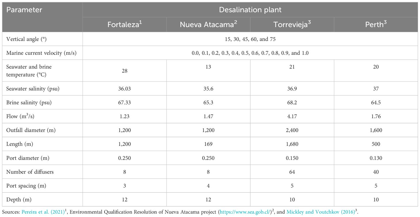
Table 1 Outfall characteristics, marine current velocities, and vertical angles used in the different modeled scenarios.
Fifty-five scenarios were simulated for each outfall, with the vertical inclination of the diffusers being changed between 15° and 75° and the velocity of the marine currents from 0.0 to 1 m/s (Table 1). In all cases, the rate of brine flow was the maximum described by Mickley and Voutchkov (2016); Pereira et al. (2021), or the Environmental Qualification Resolution of the Nueva Atacama project (https://www.sea.gob.cl/); the average salinity values reported in these studies were used for the salinity of the seawater and brine.
The results produced by the UM3 model were used to construct a multiple logarithmic and polynomial regression, which was used to calculate the dilution generated by marine currents. We tested the variables described by Bleninger et al. (2010) to choose those that had a better regression.
To validate the results of the SisBaHiA model, we again used the UM3 model to simulate the near-field dilution under the same conditions used for the proposed SisBaHiA model.
The UM3 model was chosen here considering its results for a study in which different models were compared. Loya-Fernández et al. (2012) reported good agreement between the results obtained using the UM3 model and field measurements. They concluded that UM3 was the most realistic of the mixing models that were tested.
2.3 Far-field model
After the brine jet collapses at the point where it impacts the seabed, the plume formed by this initial dilution is transported to the far field. To describe this stage, we used a Lagrangian model that included the water level and current velocity data generated by the hydrodynamic model; these data varied in space and time. In this study, an environment where currents were present and a multiport diffuser pipe with a range of possible diffuser inclination angles were included in the model as well as the far-jet diameter and a port space factor. The degree of brine dilution at the impact point, calculated from the near-field formulation given above, was used to calculate the corresponding mass of the saline concentrate and was subsequently used in the Lagrangian model.
In the Lagrangian model, the mass transport of the saline concentrate was simulated by the movement of a given number of particles randomly released within a source region in the near field at regular time intervals, with these particles being transported by the currents generated by the hydrodynamic model. The particle paths were calculated as the sum of a deterministic component (advection) and an independent random component (turbulent diffusion). The velocities calculated by the hydrodynamic model were used to simulate the advective component, whereas the diffuse component was represented by small random displacements of the particles’ centers of mass (Horita and Rosman, 2006).
The position of any particle at an instant Pn + 1 can be determined using the Taylor series expansion of the previous known position, Pn (Equation 8):
After calculating the position of the particle, the effects of the diffuse velocity field can be accounted for as random deviations from this position. These random deviations can be calculated from the spatial derivatives of turbulent diffusivities (Rosman, 2023).
In the Lagrangian model, the concentration was calculated based on a grid inside which the entire contaminant plume was contained. Once the masses of all the particles distributed across the grid cells had been calculated, the concentration in each cell was calculated as simply the mass of substance in the cell divided by the volume of the cell. A grid of this type can be constructed independently of the hydrodynamic mesh (Rosman, 2023). Once the position of a given particle at a given time is known, the particle mass is distributed to each associated grid cell according to a specific distribution function. In the simplest case, all the mass is associated with the cell where the particle is located. This applies when the cell volume is large in relation to the plume associated with a given particle. When the plume volume is large in relation to the cell size, the use of a Gaussian-type function (Horita and Rosman, 2006) may be more appropriate (Equation 9):
According to the method of moments, variances can be related to diffusivities (Fischer et al., 1979) (Equation 10):
Given that the near-field flow exists for only a few minutes, the kinetic reactions of the seven non-conservative constituents of the effluent are irrelevant. Therefore, in the case of a non-conservative constituent, only the far-field transport includes kinetic reactions.
To evaluate the integration of the near-field tool with the other modules of SisBaHiA (the hydrodynamic module, wave propagation module, and Lagrangian transport model) and with the aim of simulating the dispersion of desalination plumes in the far field, we chose a submarine outfall located at Fortaleza, Ceará State, Brazil. A desalination plant is to be constructed at this location, which is one of the four cases listed in Table 1. For that, a calibration step was included in this work to validate the hydrodynamic model results (sea level, current intensity and direction).
2.4 Metocean data
Bathymetric data for Fortaleza were obtained from nautical charts produced by the Brazilian Navy Hydrographic Center (Figure 1). A set of 33 tidal harmonic constants obtained from the Finite Element Solution (FES) at two stations was used to calculate the astronomical sea level at the boundary condition (Figure 2); the non-astronomical sea-level variations were not included since they were not important in the region and because the astronomical components were higher than them. Five stations of wind and one of wave data were used to force the model (Figure 1), and these were obtained from the atmospheric reanalysis model ERA5 (Hersbach et al., 2020) produced by the European Centre for Medium-Range Weather Forecasts (ECMWF) (Figure 3). Currents, originating outside the modeled region, were incorporated into the hydrodynamic model using reanalysis data from the Hybrid Coordinate Ocean Model (HYCOM), as presented by de Andrade et al. (2019). Figure 1 shows the locations of all station data mentioned above, the mesh of finite elements used for this demonstration study, the brine outfall, and the water intake point. For this test case, we used weather conditions for a representative month (October).
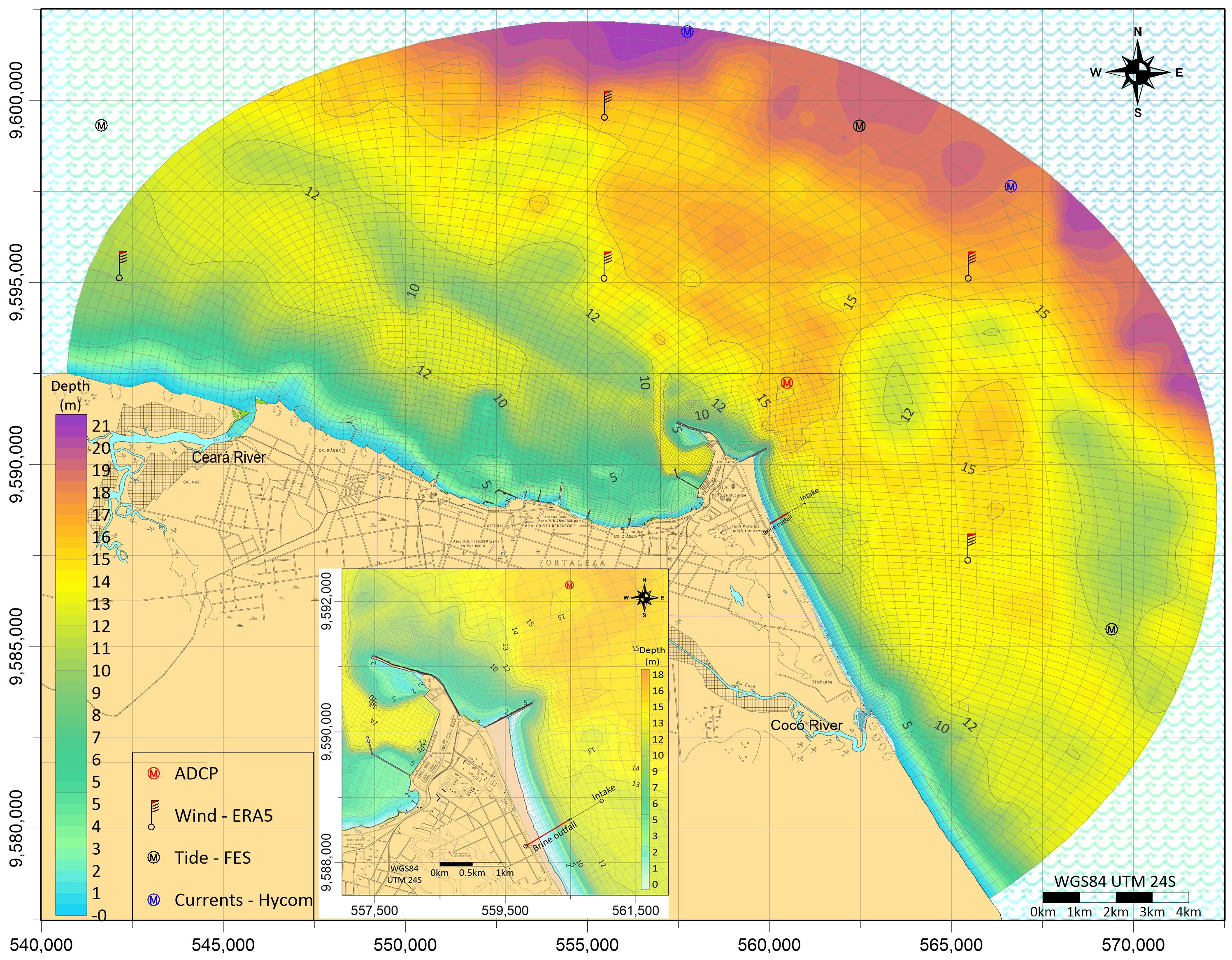
Figure 1 Biquadratic finite element mesh with 1,985 elements and 8,215 calculation nodes used for the domain discretization and bathymetry in meters relative to local chart datum for Fortaleza, Brazil.

Figure 2 Tide elevation at Fortaleza during October 2021 generated from the FES.
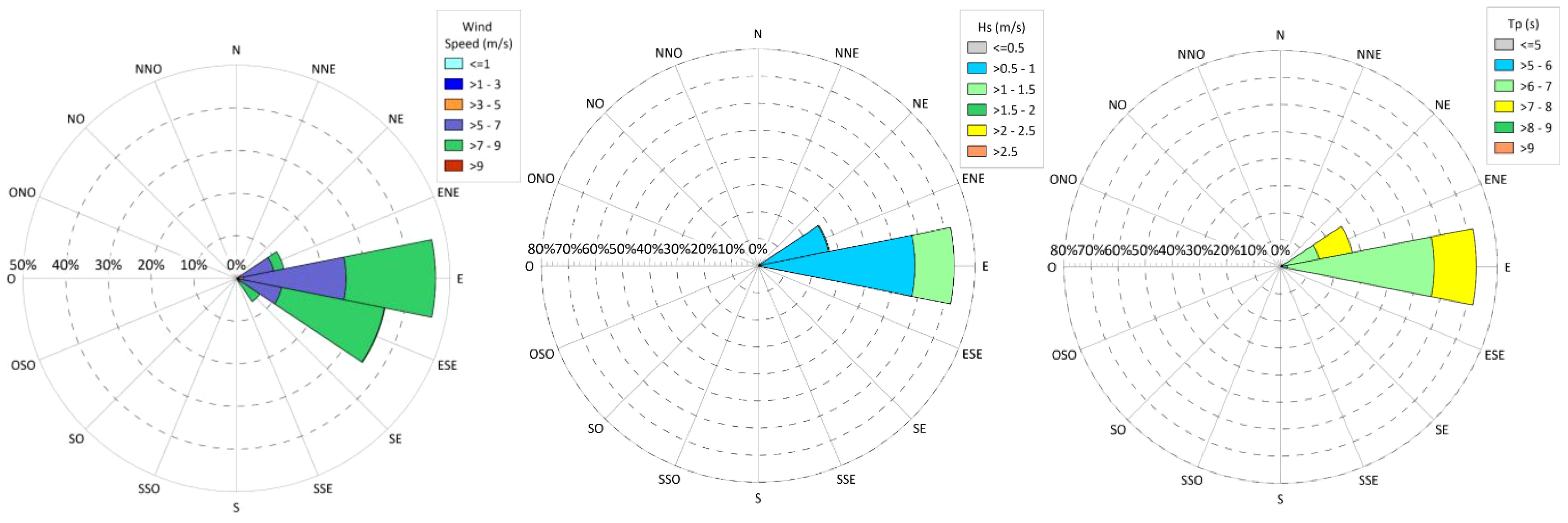
Figure 3 Wind and wave roses during October 2021 obtained from the ECMWF. Hs is the wave height and Tp is the peak wave period.
2.5 Calibration of the hydrodynamic model
The capacity of a model to reproduce realistic results depends on the calibration process. For hydrodynamic models, this involves correctly defining the boundary conditions (e.g., tides, winds, and roughness) and sometimes downscaling the velocity fields at open boundaries from large-scale hydrodynamic models.
Herein, a three-dimensional hydrodynamic model was chosen, because it considers major physical drivers, such as astronomical tides, winds, and waves. To represent the pattern of littoral currents, a series of differential mean levels were prescribed as an additional boundary condition along the open boundaries using currents from the large-scale HYCOM model.
To calibrate and validate the hydrodynamic model, we used real data measured over 9 months, obtained using an Acoustic Doppler Current Profiler (ADCP) deployed near the outfall area (Figure 1). From these data, we obtained depth-averaged current speeds and directions, as well as sea-level elevations, for comparison with the simulated data.
3 Results
The fundamental parameter to be obtained in studies of diffuser systems is the minimum dilution reached at the end of the near field. This dilution must be large enough to comply with environmental standards so that environmental impacts do not occur at this distance (Bleninger and Jirka, 2011).
Figures 4–7 show the initial dilution obtained for different diffuser vertical angles using the SisBaHiA and Visual Plumes models. The dashed lines (SisBaHiA initial dilution) were calculated using the regression coefficients obtained previously. For a quiescent condition, the methodology of Bleninger et al. (2010) was adopted. The minimum dilution gradually increases as both the launch angle and the marine current velocity increase, as observed in previous experimental and numerical studies (Cipollina et al., 2005; Palomar et al., 2012; Ximenes et al., 2023). The dilution obtained using SisBaHiA is very close to that derived using Visual Plumes, especially for vertical angles between 45° and 60°. Figure 8 shows a comparison between the SisBaHiA and Visual Plumes results for all the cases; the coefficient of determination is very high (R2 > 0.95). The good reproducibility of the initial dilution can also be inferred from the low value of the mean absolute percentage error (MAPE) (9%), and more than 95% of the differences between the two sets of results are below 22%.
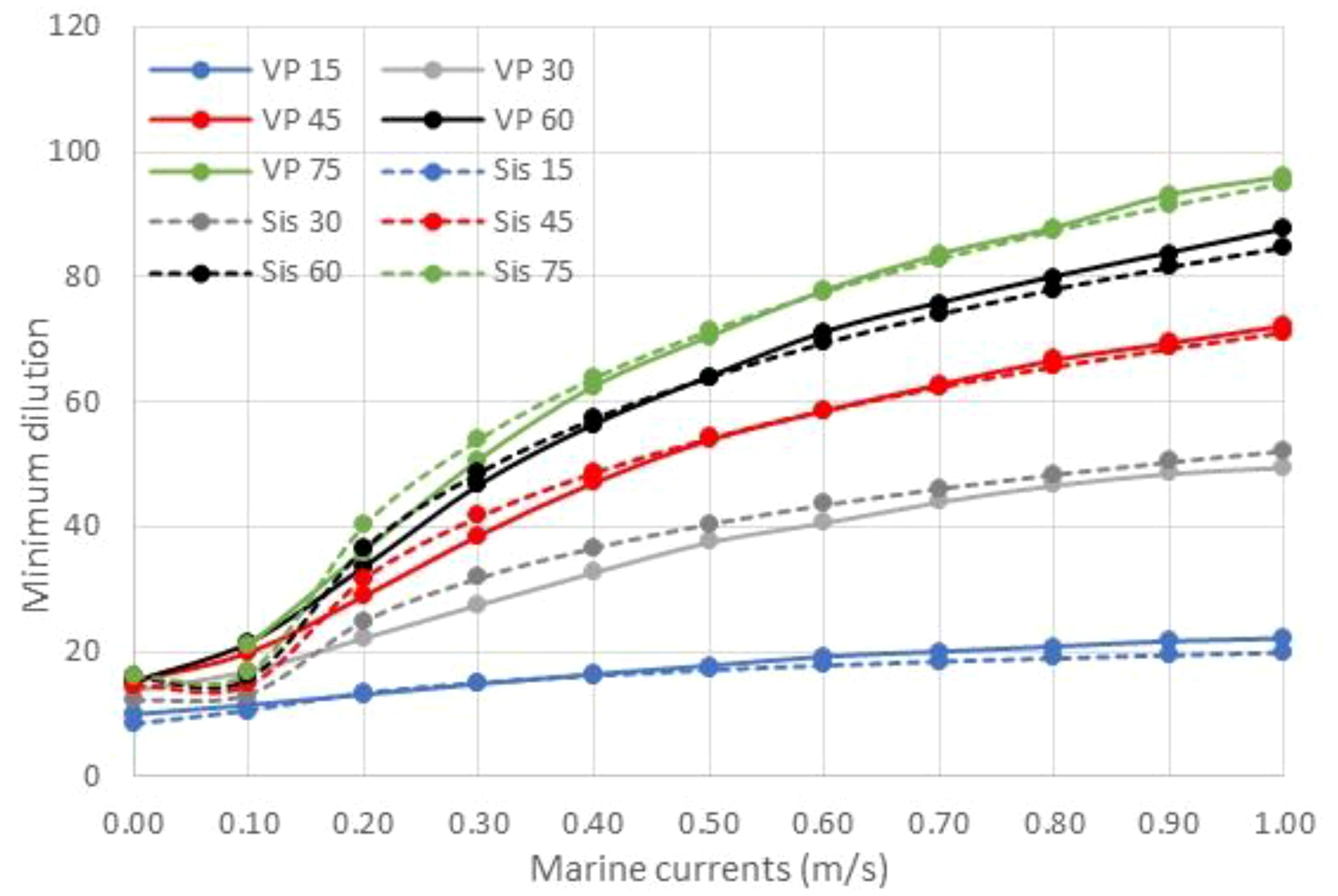
Figure 4 Minimum dilution at the near field for different diffuser vertical angles produced by the Visual Plumes (VP) and SisBaHiA (Sis) models for the Fortaleza desalination plant.
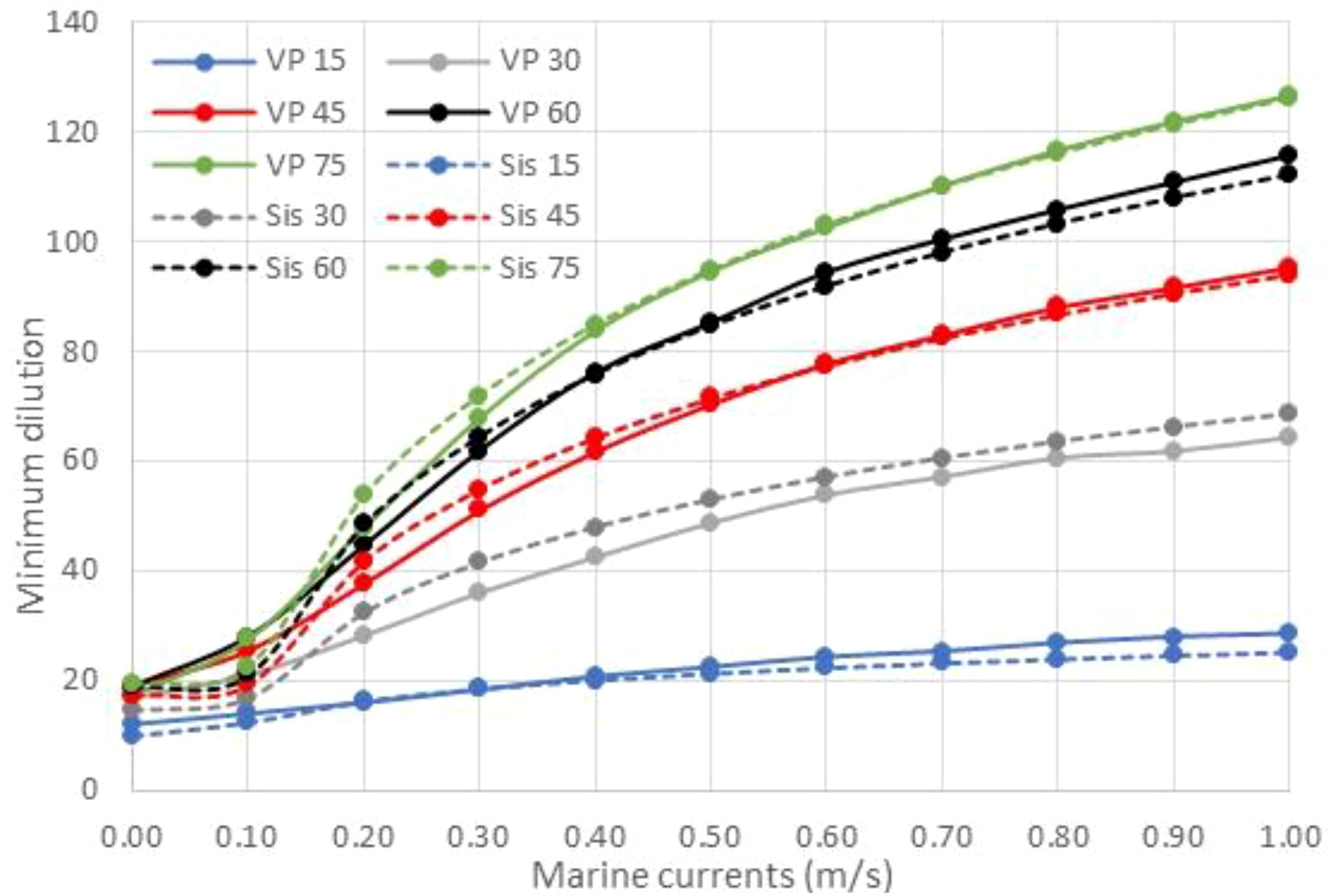
Figure 5 Minimum dilution at the near field for different diffuser vertical angles produced by the Visual Plumes (VP) and SisBaHiA (Sis) models for the Nueva Atacama desalination plant.
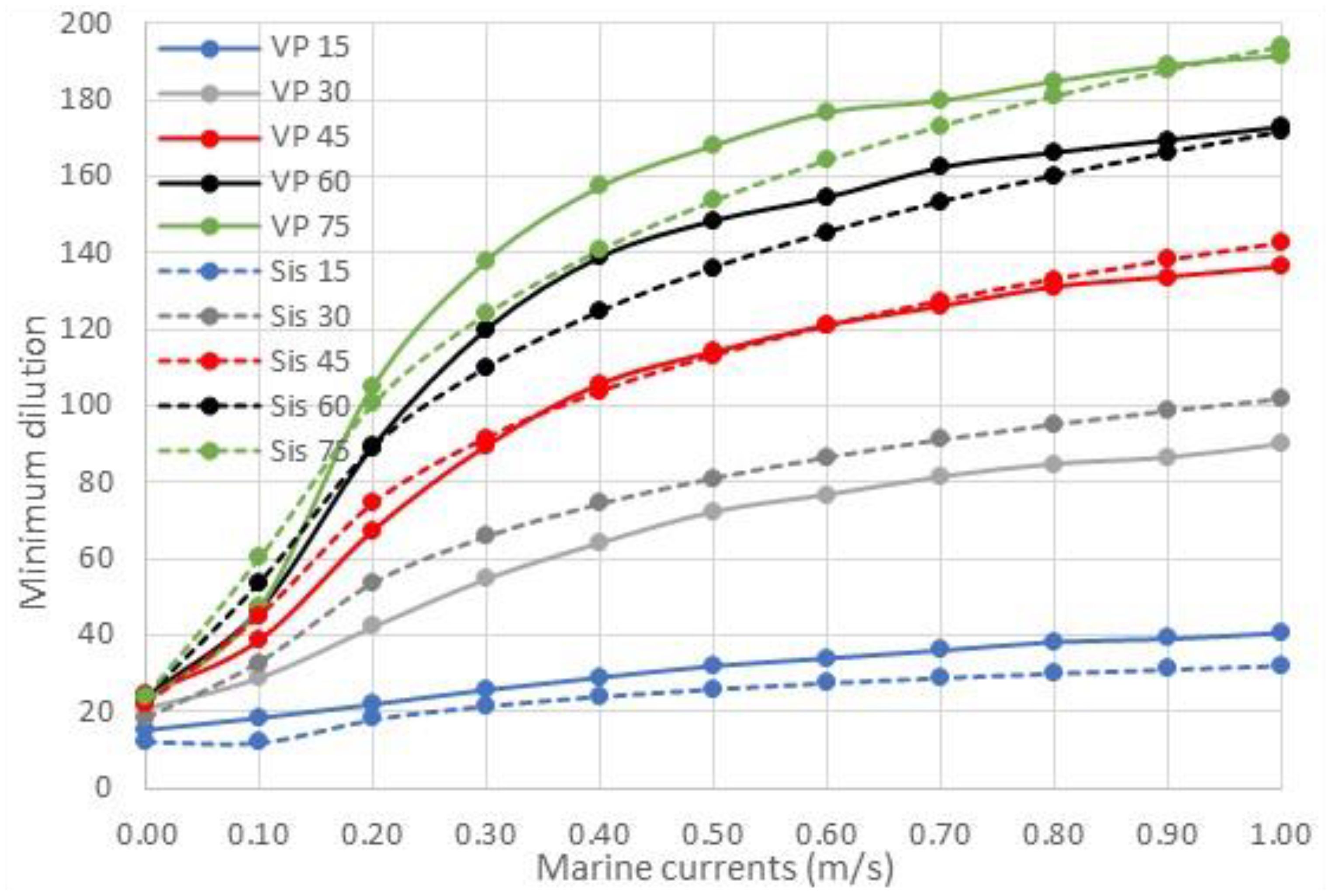
Figure 6 Minimum dilution at the near field for different diffuser vertical angles produced by the Visual Plumes (VP) and SisBaHiA (Sis) models for the Torrevieja desalination plant.
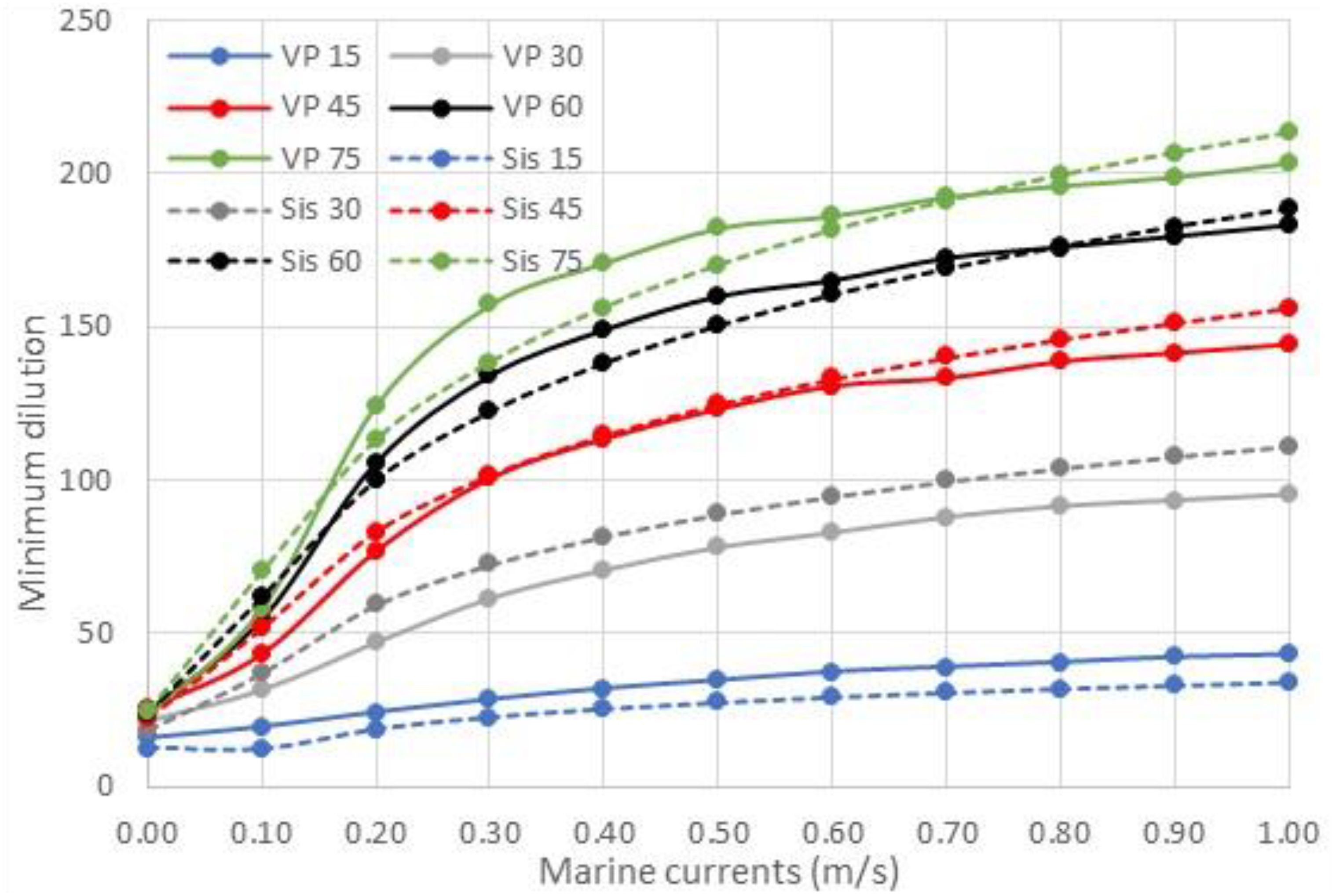
Figure 7 Minimum dilution at the near field for different diffuser vertical angles produced by the Visual Plumes (VP) and SisBaHiA (Sis) models for the Perth desalination plant.
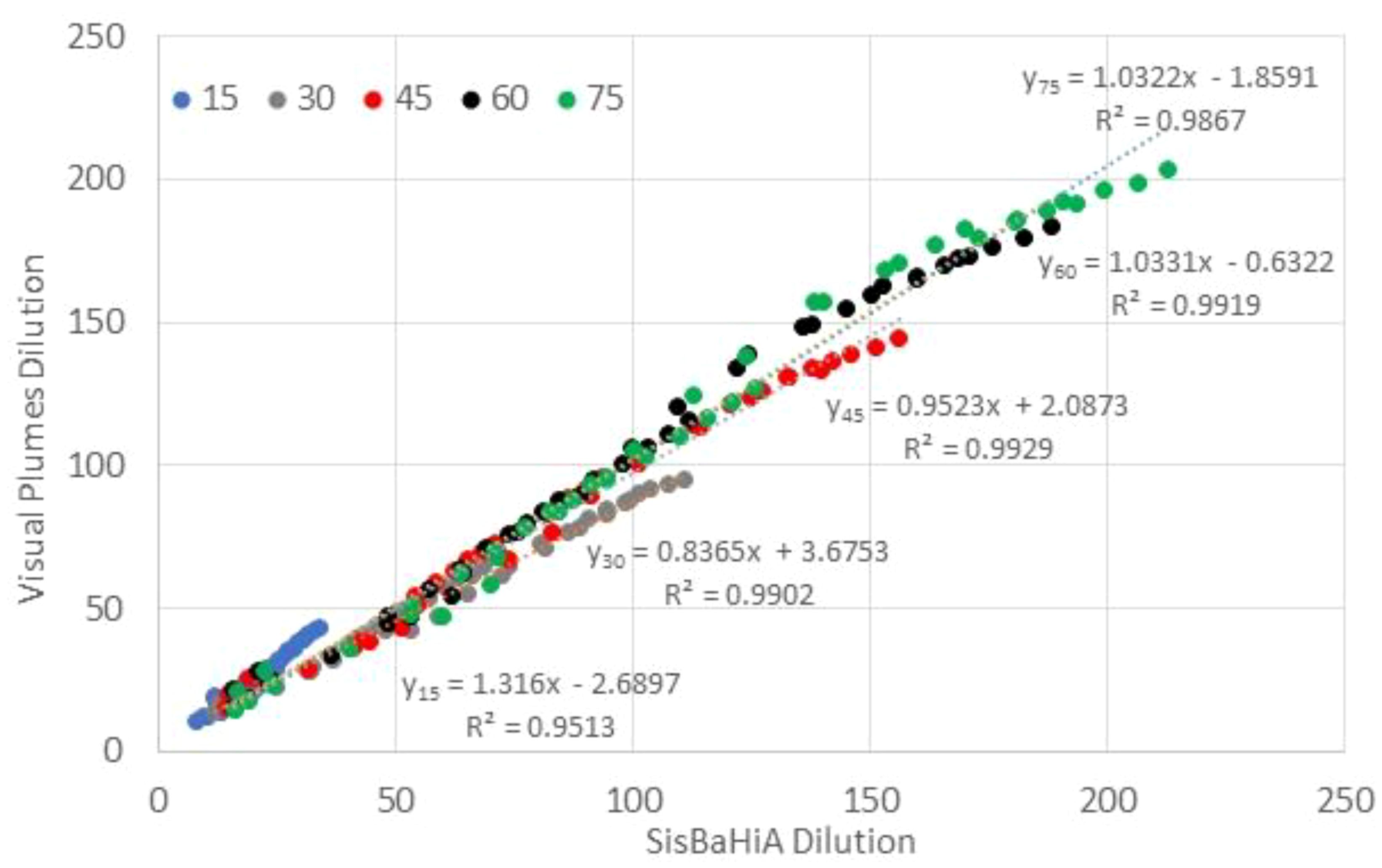
Figure 8 Correlation between minimum dilution generated by the SisBaHiA and Visual Plumes models for different diffuser vertical angles and marine current velocities for the four desalination plants.
If we consider only the vertical angles used by the outfall projects listed in Section 2.2, the MAPE between the two sets of results is only 5%. For these cases, the initial dilutions calculated by SisBaHiA range from 15 to 71 for Fortaleza, 17 to 94 for Nueva Atacama, 22 to 142 for Torrevieja, and 22–156 for Perth for marine current velocities in the range of 0.0–1.0 m/s (Table 2).
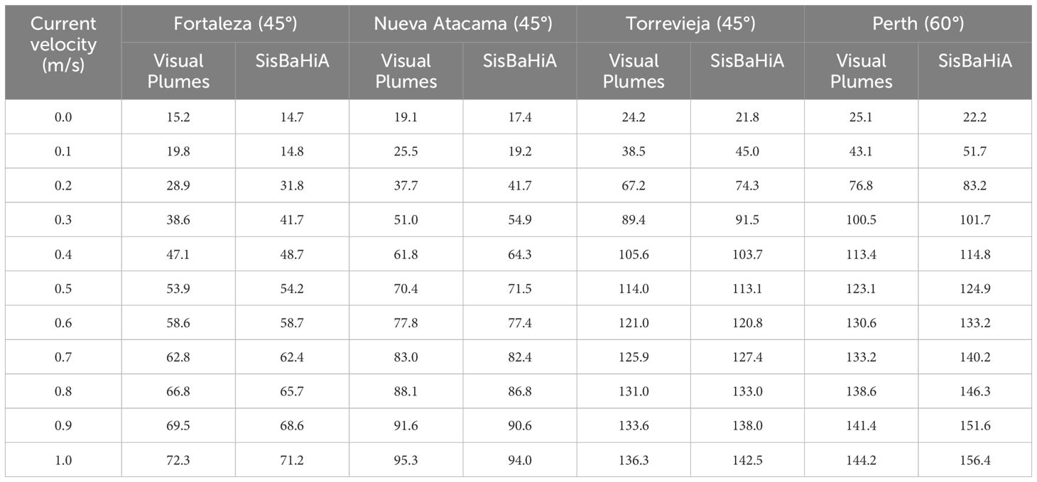
Table 2 Near-field dilution values obtained using the SisBaHiA and Visual Plumes models for the diffuser vertical angles adopted by each outfall project.
In Figure 9, we see the marine current behavior measured by the ADCP and produced by the hydrodynamic model at the ADCP deployed point, at 2 m from the bottom. For both cases, the average current speed was very similar, 0.29 m/s for the ADCP and 0.30 m/s for the model. The current speed range varied from 0.08 to 0.59 m/s for the ADCP and from 0.04 to 0.49 m/s for the model.
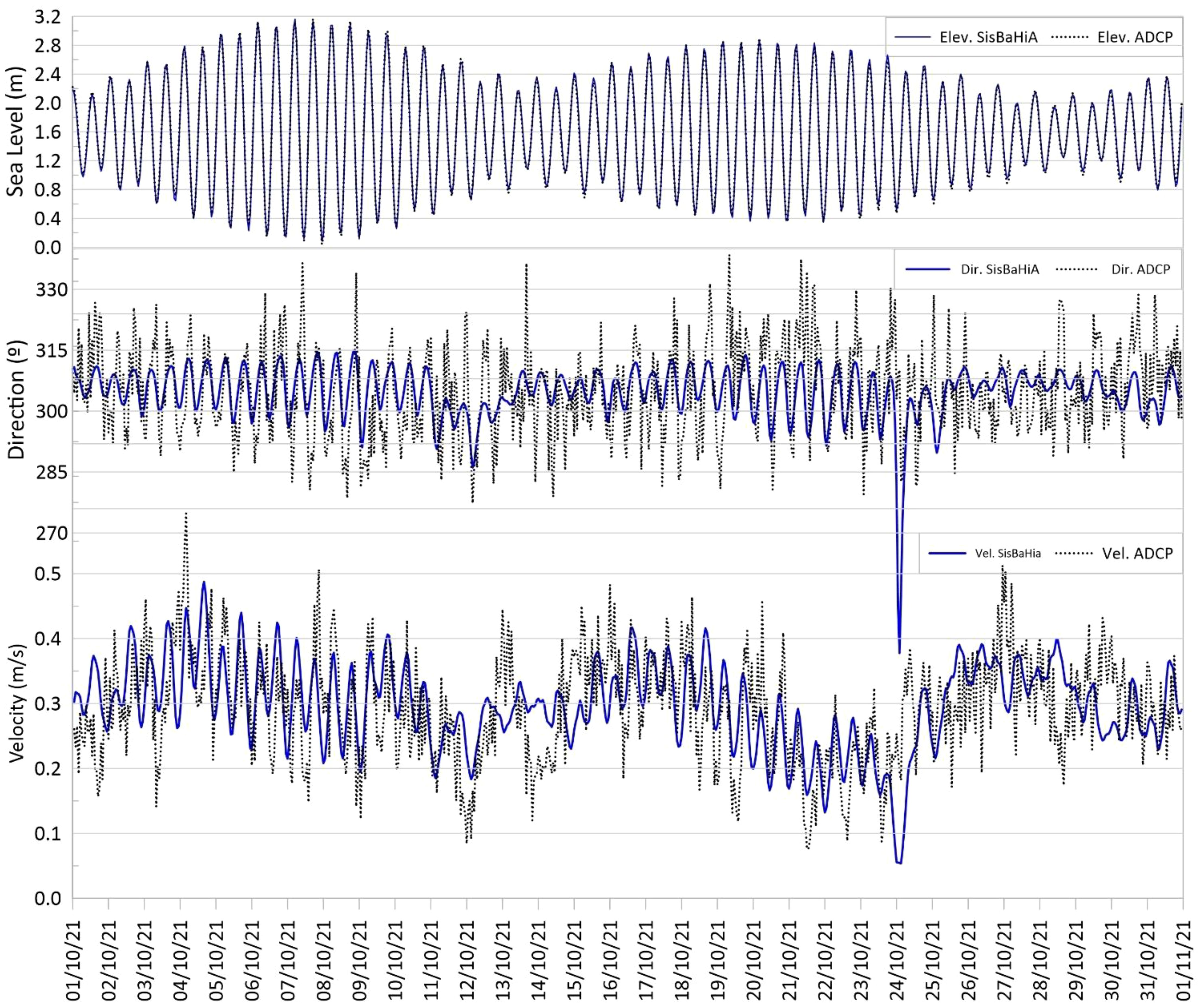
Figure 9 Sea elevation, velocity, and direction of marine currents produced by the hydrodynamic model and measured with the ADCP at the same place.
The hydrodynamic model results, along with the measured data, show a tendency for marine currents to flow westward, following the main wind direction and bathymetry orientation (Figure 10, left). In some situations, the nearshore alongshore current direction changed to an eastward direction driven by easterly waves (Figure 10, right). Nearshore alongshore currents, which are wave-generated currents acting along the wave-breaking zone, are highly dependent on the direction of incident waves and its interaction with the jets present in the area, as reported by Pereira et al. (2021). Near the outfall diffusers, the average current speed was 0.22, ranging from 0.18 to 0.27 m/s.
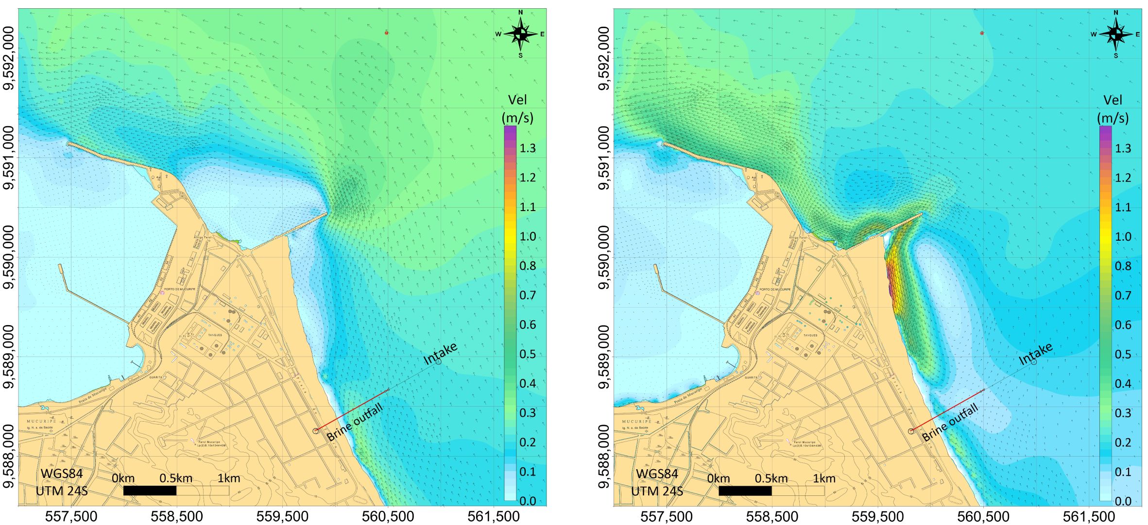
Figure 10 Typical currents in the area (left) and with an East Wave influence (right).
Figure 11 shows the results obtained using the SisBaHiA Lagrangian transport model coupled with the near-field model for Fortaleza. On the left side, we see the saline plume spreading in a usual environmental situation, while on the right side, we see changes led by eastward currents (Figure 10, right), switching the plume direction from an almost northward to a northeastward direction.
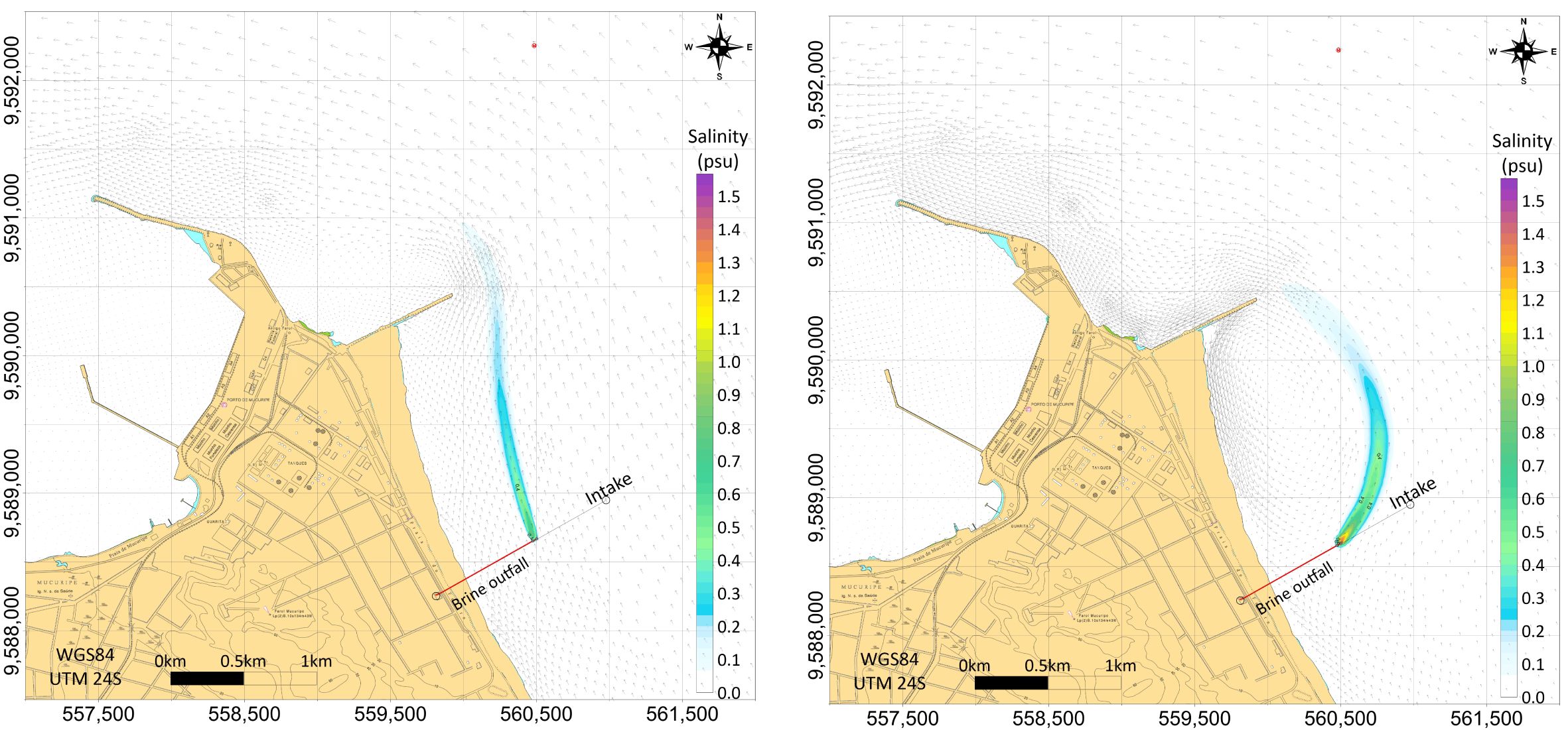
Figure 11 Typical saline plume behavior (left) and changes affected by an East Wave influence (right).
Figure 12 shows the probabilities of the salinity exceeding the maximum acceptable value according to the transport model results for the entire month of October 2021. We used as a reference the most restricted value reported by Pereira et al. (2021), 0.8 psu with a compliance distance of 1 km. For up to 50% of the time, this value was exceeded within the limited region less than 100 m from the diffusers. As the effluent spreads in the ambient receiving water, this exceedance time decreases to less than 1% of that month and at approximately 1 km from the diffusers.
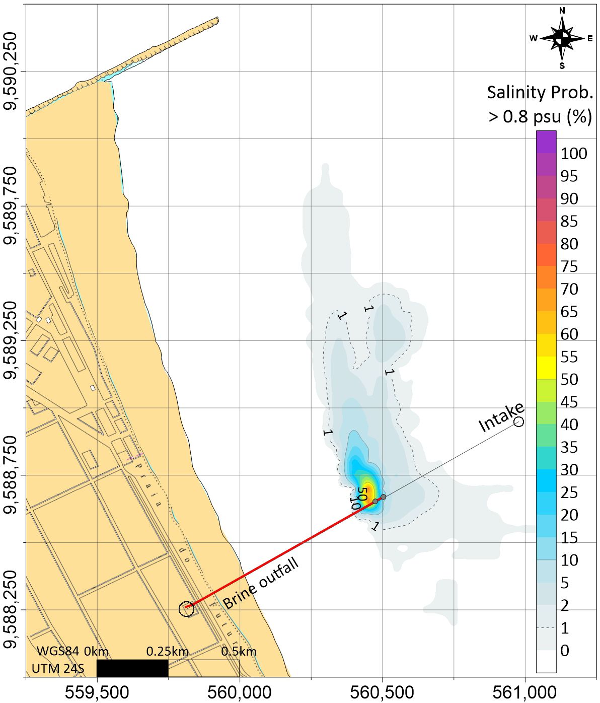
Figure 12 Probability of the salinity exceeding a reference acceptable value (0.8 psu) according to the transport model results for October 2021.
4 Discussion
The increasing demand for fresh water in many regions of the world highlights the importance of using desalination as a means of addressing water scarcity (Eke et al., 2020). However, appropriate mitigation strategies and measures are necessary for the sustainable development of this technology (Fernández-Torquemada et al., 2019; Sola et al., 2020). Between the mitigation strategies, actions to ensure a proper dilution of the brine are probably the most relevant (Fernández-Torquemada et al., 2019). In this study, we have presented the first results obtained using a new SisBaHiA Lagrangian model for modeling the behavior of brine discharges in the marine environment.
To implement and evaluate the near-field dilution model, four desalination plants currently in operation or planned were taken as case studies, under different environmental conditions worldwide. These desalination plants included one site chosen to construct a new plant at Fortaleza City, Brazil; the Torrevieja desalination plant on the Mediterranean coast of Spain; the Nueva Atacama desalination plant at the Pacific Coast of Chile; and the Perth City desalination plant in Australia.
A good correlation and low error were obtained when we constructed the multiple logarithmic and polynomial regression using the following independent variables: marine currents, vertical angle of the diffusers, initial momentum flux, and initial buoyancy flux. The dilution presented a logarithmic behavior with marine currents and vertical angle, while the other two variables behaved linearly. The definitions of initial momentum and buoyancy fluxes are given by Bleninger et al. (2010). Note that the higher dilution of the jet in crossflow compared to that of a free jet in stagnant ambient is a result of induced shear layers, vortex dynamics, increased turbulence, and the geometric effects of jet deflection and spreading. Therefore, the crossflow actively promotes more effective entrainment and mixing, resulting in greater dilution of the jet fluid, as stated by Jirka (2004).
The novelty of this approach was the dynamic coupling of a near-field model with a far-field model, focusing on dense discharges and coupling with Lagrangian modeling approaches. Additionally, the incorporation of a wave model in coastal hydrodynamic simulations was also innovative.
In the context of the sustainable development of desalination, it is important to ensure proper dilution of discharged effluents to reduce the area affected by these discharges and thus minimize the impact on marine ecosystems (Sharifinia et al., 2019). To ensure optimal dilution, it is important to adopt a good design for the discharge outfall; the results of this study demonstrate how computational tools are useful in optimizing this design. For example, our results indicate that the best dilution of all four plants is achieved with diffuser vertical angles between 60° and 75°; for these angles, near-field lengths of less than 12 m were found.
To validate the model, comparisons with measured data were undertaken for the Fortaleza case study. The similarity between the measured and modeled sea levels was excellent in terms of both amplitude and phase (Figure 9). Moreover, the general patterns of the velocity and direction of marine currents produced by the hydrodynamic model closely matched those measured, demonstrating the reliability of the model for the prediction of related parameters.
According to our results, the SisBaHiA near-field model produces similar dilution results to those produced by the Visual Plumes software. The mean deviation between the two sets of results obtained for a range of seawater salinities and temperatures, marine current velocities, brine salinities, and diffuser numbers and characteristics was 9%. However, the SisBaHiA software has some advantages compared with other computational models. First, this model includes both the near- and far-field dynamics, whereas other models are concerned with only either the near field or the far field. Additionally, the coupled wave propagation model permits the analysis of changes in the brine plume direction produced by waves formed far from the outfall area. The effects of these waves on the current field can change the plume dispersion, as demonstrated in this work.
Moreover, using SisBaHiA, it is possible to couple a dispersion model to a baroclinic hydrodynamic model (Cunha et al., 2018; de Andrade et al., 2019), thus enabling the simulation of density currents produced by salinity and/or temperature gradients created in the outfall area. Finally, the sophistication of the Lagrangian model, which included an anisotropic Gaussian distribution of particles together with random diffusion that was proportional to the turbulence gradient and the advection, allowed more realistic solutions to be obtained. It is also important to advance the development of new field studies with the aim of validating the theoretical data obtained with the model against the measured data of the evaluated case studies (Loya-Fernández et al., 2012).
5 Conclusion
In this study, the initial dilution of brine effluent discharged from desalination plants was modeled by a novel SisBaHiA Lagrangian model as well as by the Visual Plumes software. The results obtained using the two models were similar, especially for diffuser vertical angles of 45° and 60°. However, the SisBaHiA Lagrangian model has some advantages over other computational models and provides an effective tool for evaluating the dispersion of brine discharges from desalination plants. Regarding the four cases that were studied, the best results were obtained for diffuser angles of between 60° and 75° as at these angles the dilution was the greatest, and near-field lengths of less than 12 m from the diffusion line could be achieved. The coupled wave propagation model permitted the analysis of changes in the brine plume direction produced by waves formed far from the outfall area, as shown in the example case. In addition, it is important to emphasize that the modeling tool that was tested in this study is of international relevance as it can be applied to any part of the world and to consider the different technical characteristics of individual desalination plants as well as local environmental conditions. Given the expected global expansion of the use of desalination, the adoption of scientifically tested measures, such as the SisBaHiA Lagrangian model, will become ever more important. The application of this tool will facilitate the implementation of optimal logistical strategies and efficient discharge configurations, thus ensuring the effective minimization of the environmental impact of the desalination industry worldwide.
Data availability statement
Publicly available datasets were analyzed in this study. This data can be found here: https://www.ecmwf.int/en/forecasts/dataset/ecmwf-reanalysis-v5.
Author contributions
SP: Conceptualization, Investigation, Methodology, Writing – original draft, Writing – review & editing. MR: Investigation, Writing – original draft. PCCR: Formal analysis, Methodology, Supervision, Writing – review & editing. PR: Software, Writing – review & editing. TB: Formal analysis, Methodology, Supervision, Writing – review & editing. IL: Funding acquisition, Supervision, Validation, Writing – review & editing. CT: Writing – review & editing, Formal analysis, Resources. IS: Writing – review & editing, Validation. JS: Resources, Supervision, Writing – review & editing.
Funding
The author(s) declare financial support was received for the research, authorship, and/or publication of this article. We thank the National Council for Scientific and Technological Development, CNPq (research fellowship no. 200277/2022–7). Tobias Bleninger acknowledges the productivity stipend from the National Council for Scientific and Technological Development – CNPq, grant no. 313491/2023–2, call no. 09/2023 and Carlos Teixeira CNPq grant 315289/2021–0 and FUNCAP grant UNI-0210–00542.01.00/23.
Conflict of interest
The authors declare that the research was conducted in the absence of any commercial or financial relationships that could be construed as a potential conflict of interest.
Publisher’s note
All claims expressed in this article are solely those of the authors and do not necessarily represent those of their affiliated organizations, or those of the publisher, the editors and the reviewers. Any product that may be evaluated in this article, or claim that may be made by its manufacturer, is not guaranteed or endorsed by the publisher.
References
Barros M. d. L. C., Rosman P. C. C. (2018). A study on fish eggs and larvae drifting in the Jirau reservoir, Brazilian Amazon. J. Braz. Soc. Mechanical Sci. Eng. 40, 62. doi: 10.1007/s40430-017-0951-1
Belatoui A., Bouabessalam H., Hacene O. R., de-la-Ossa-Carretero J. A., Martinez-Garcia E., Sanchez-Lizaso J. L. (2017). Environmental effects of brine discharge from two desalinations plants in Algeria (South Western Mediterranean). Desalination Water Treat 76, 311–318. doi: 10.5004/dwt.2017.20812
Bleninger T. (2007). Coupled 3D hydrodynamic models for submarine outfalls: Environmental hydraulic design and control of multiport diffusers. Diss. Inst. Hydromech. 2006, 7–27. doi: 10.5445/KSP/1000006668
Bleninger T., Jirka G. H. (2008). Modelling and environmentally sound management of brine discharges from desalination plants. Desalination 221, 585–597. doi: 10.1016/j.desal.2007.02.059
Bleninger T., Jirka G. H. (2011). Mixing zone regulation for effluent discharges into EU waters. Proc. Institution Civil Engineers - Water Manage. 164, 387–396. doi: 10.1680/wama.900037
Bleninger T., Niepelt A., Jirka G. (2010). Desalination plant discharge calculator. Desalination Water Treat 13, 156–173. doi: 10.5004/dwt.2010.1055
Cipollina A., Brucato A., Grisafi F., Nicosia S. (2005). Bench-scale investigation of inclined dense jets. J. Hydraulic Eng. 131, 1017–1022. doi: 10.1061/(ASCE)0733-9429(2005)131:11(1017
Cunha C. D. L., da N., Corrêa G. P., Rosman P. C. C. (2018). A coupled model of hydrodynamics circulation and water quality applied to the Rio Verde reservoir, Brazil. Ambiente e Agua - Interdiscip. J. Appl. Sci. 13, 1. doi: 10.4136/ambi-agua.2244
de Andrade V. S., Rosman P. C. C., de Azevedo J. P. S. (2019). Evaluation of baroclinic effects on mean water levels in Guanabara Bay. RBRH 24, e48. doi: 10.1590/2318-0331.241920180112
Del-Pilar-Ruso Y., Martinez-Garcia E., Giménez-Casalduero F., Loya-Fernández A., Ferrero-Vicente L. M., Marco-Méndez C., et al. (2015). Benthic community recovery from brine impact after the implementation of mitigation measures. Water Res. 70, 325–336. doi: 10.1016/j.watres.2014.11.036
Eke J., Yusuf A., Giwa A., Sodiq A. (2020). The global status of desalination: An assessment of current desalination technologies, plants and capacity. Desalination 495, 114633. doi: 10.1016/j.desal.2020.114633
Feitosa R. C., Rosman P. C. C., Bleninger T., Wasserman J. C. (2013). Coupling bacterial decay and hydrodynamic models for sewage outfall simulation. J. Appl. Water Eng. Res. 1, 137–147. doi: 10.1080/23249676.2013.878882
Fernández-Torquemada Y., Carratalá A., Sánchez Lizaso J. L. (2019). Impact of brine on the marine environment and how it can be reduced. Desalination Water Treat 167, 27–37. doi: 10.5004/dwt.2019.24615
Fernández-Torquemada Y., Gónzalez-Correa J. M., Loya A., Ferrero L. M., Díaz-Valdés M., Sánchez-Lizaso J. L. (2009). Dispersion of brine discharge from seawater reverse osmosis desalination plants. Desalination Water Treat 5, 137–145. doi: 10.5004/dwt.2009.576
Fischer H. B., List E. J., Koh R. C. Y., IMBERGER J., BROOKS N. H. (1979). “Turbulent diffusion,” in Mixing in Inland and Coastal Waters (Elsevier), 55–79. doi: 10.1016/B978-0-08-051177-1.50007-6
Frick W. E. (2004). Visual Plumes mixing zone modeling software. Environ. Model. Softw. 19, 645–654. doi: 10.1016/j.envsoft.2003.08.018
Heck N., Paytan A., Potts D. C., Haddad B., Lykkebo Petersen K. (2018). Management preferences and attitudes regarding environmental impacts from seawater desalination: Insights from a small coastal community. Ocean Coast. Manag. 163, 22–29. doi: 10.1016/j.ocecoaman.2018.05.024
Hersbach H., Bell B., Berrisford P., Hirahara S., Horányi A., Muñoz-Sabater J., et al. (2020). The ERA5 global reanalysis. Q. J. R. Meteorological Soc. 146, 1999–2049. doi: 10.1002/qj.3803
Horita C. O., Bleninger T. B., Morelissen R., de Carvalho J. L. B. (2019). Dynamic coupling of a near with a far field model for outfall discharges. J. Appl. Water Eng. Res. 7, 295–313. doi: 10.1080/23249676.2019.1685413
Horita C., Rosman P. (2006). A Lagrangian model for shallow water bodies contaminant transport. J. Coast. Res. 39, 1610–1613.
Hunt G. R., Burridge H. C. (2015). Fountains in industry and nature. Annu. Rev. Fluid Mech. 47, 195–220. doi: 10.1146/annurev-fluid-010313-141311
IAEA (2019). Modelling of marine dispersion and transfer of radionuclides accidentally released from land . based facilities (INTL ATOMIC ENERGY AGENCY).
Jirka G. H. (2004). Integral model for turbulent buoyant jets in unbounded stratified flows. Part I: single round jet. Environ. Fluid Mech. 4, 1–56. doi: 10.1023/A:1025583110842
Kirby J. T., Dalrymple R. A., Shi F. (2002). Combined Refraction/diffraction Model REF/DIF 1: Documentation and User’s Manual. 3rd Edn (Newark: Center for Applied Coastal Research, Department of Civil Engineering, University of Delaware). Available at: https://books.google.com.br/books?id=I3ZoQwAACAAJ.
Lattemann S., Höpner T. (2008). Environmental impact and impact assessment of seawater desalination. Desalination 220, 1–15. doi: 10.1016/j.desal.2007.03.009
Loya-Fernández Á., Ferrero-Vicente L. M., Marco-Méndez C., Martínez-García E., Zubcoff J., Sánchez-Lizaso J. L. (2012). Comparing four mixing zone models with brine discharge measurements from a reverse osmosis desalination plant in Spain. Desalination 286, 217–224. doi: 10.1016/j.desal.2011.11.026
Loya-Fernández Á., Ferrero-Vicente L. M., Marco-Méndez C., Martínez-García E., Zubcoff Vallejo J. J., Sánchez-Lizaso J. L. (2018). Quantifying the efficiency of a mono-port diffuser in the dispersion of brine discharges. Desalination 431, 27–34. doi: 10.1016/j.desal.2017.11.014
Mickley M., Voutchkov N. (2016). Database of permitting practices for seawater concentrate disposal. Water Intell. Online 15, 9781780408484. doi: 10.2166/9781780408484
Morelissen R., van der Kaaij T., Bleninger T. (2013). Dynamic coupling of near field and far field models for simulating effluent discharges. Water Sci. Technol. 67, 2210–2220. doi: 10.2166/wst.2013.081
Palomar P., Lara J. L., Losada I. J., Rodrigo M., Alvárez A. (2012). Near field brine discharge modelling part 1: Analysis of commercial tools. Desalination 290, 14–27. doi: 10.1016/j.desal.2011.11.037
Peixoto R., dos S., Rosman P. C. C., Vinzon S. B. (2017). A morphodynamic model for cohesive sediments transport. RBRH 22, e57. doi: 10.1590/2318-0331.0217170066
Pereira S. P., Rosman P. C. C., Alvarez C., Schetini C. A. F., Souza R. O., Vieira R. H. S. F. (2015). Modeling of coastal water contamination in Fortaleza (Northeastern Brazil). Water Sci. Technol. 72, 928–936. doi: 10.2166/wst.2015.292
Pereira S. P., Rosman P. C. C., Sánchez-Lizaso J. L., Neto I. E. L., Silva R. A. G., Rodrigues M. (2021). Brine outfall modeling of the proposed desalination plant of fortaleza, Brazil. Desalination Water Treat 234, 22–30. doi: 10.5004/dwt.2021.27557
Pistocchi A., Bleninger T., Dorati C. (2020). Screening the hurdles to sea disposal of desalination brine around the Mediterranean. Desalination 491, 114570. doi: 10.1016/j.desal.2020.114570
Purnama A., Al-Barwani H. H., Bleninger T., Doneker R. L. (2011). CORMIX simulations of brine discharges from Barka plants, Oman. Desalination Water Treat 32, 329–338. doi: 10.5004/dwt.2011.2718
Roberts P. J. W. (2015). Near Field Flow Dynamics of Concentrate Discharges and Diffuser Design (Cham: Springer International Publishing). 369–396. doi: 10.1007/978-3-319-13203-7_17
Rosman P. C. C. (2007). “Subsídios para modelagem de sistemas estuarinos,” in Métodos Numéricos em Recursos Hídricos. Ed. Silva R. C. V. (ABHH, Porto Alegre), 238–248.
Saeedi M., Farahani A. A., Abessi O., Bleninger T. (2012). Laboratory studies defining flow regimes for negatively buoyant surface discharges into crossflow. Environ. Fluid Mech. 12, 439–449. doi: 10.1007/s10652-012-9245-4
Sawakuchi H. O., Neu V., Ward N. D., Barros M., de L. C., Valerio A. M., et al. (2017). Carbon dioxide emissions along the lower amazon river. Front. Mar. Sci. 4. doi: 10.3389/fmars.2017.00076
Sharifinia M., Afshari Bahmanbeigloo Z., Smith W. O., Yap C. K., Keshavarzifard M. (2019). Prevention is better than cure: Persian Gulf biodiversity vulnerability to the impacts of desalination plants. Glob. Chang. Biol. 25, 4022–4033. doi: 10.1111/gcb.14808
Sola I., Fernández-Torquemada Y., Forcada A., Valle C., del Pilar-Ruso Y., González-Correa J. M., et al. (2020). Sustainable desalination: Long-term monitoring of brine discharge in the marine environment. Mar. pollut. Bull. 161, 111813. doi: 10.1016/j.marpolbul.2020.111813
Ximenes L. B., Pereira S. P., Neto I. E. L. (2023). Computational fluid dynamics of marine discharge of hypersaline solution. Engenharia Sanitaria e Ambiental 28. doi: 10.1590/S1413-415220220137
Keywords: brine dilution, desalination discharge, Lagrangian model, near-field model, negative buoyancy, outfall modeling
Citation: Porto Pereira S, Rodrigues MF, Rosman PCC, Rosman P, Bleninger T, Lima Neto IE, Teixeira CEP, Sola I and Sánchez Lizaso JL (2024) A novel tool for modeling the near- and far-field dispersion of brine effluent from desalination plants. Front. Mar. Sci. 11:1377252. doi: 10.3389/fmars.2024.1377252
Received: 27 January 2024; Accepted: 27 June 2024;
Published: 29 July 2024.
Edited by:
Allan Douglas Cembella, Alfred Wegener Institute Helmholtz Centre for Polar and Marine Research (AWI), GermanyReviewed by:
Marcos D. Mateus, Universidade de Lisboa, PortugalIshita Shrivastava, Gradient, United States
Yaowen Xia, Yunnan Normal University, China
Copyright © 2024 Porto Pereira, Rodrigues, Rosman, Rosman, Bleninger, Lima Neto, Teixeira, Sola and Sánchez Lizaso. This is an open-access article distributed under the terms of the Creative Commons Attribution License (CC BY). The use, distribution or reproduction in other forums is permitted, provided the original author(s) and the copyright owner(s) are credited and that the original publication in this journal is cited, in accordance with accepted academic practice. No use, distribution or reproduction is permitted which does not comply with these terms.
*Correspondence: Silvano Porto Pereira, c2lsdmFub3BlcmVpcmFAdGVycmEuY29tLmJy