Abstract
Representing and forecasting global ocean velocities is challenging. Velocity observations are scarce and sparse, and are rarely assimilated in a global ocean configuration. Recently, different satellite mission candidates have been proposed to provide surface velocity measurements. To assess the impact of assimilating such data, Observing System Simulation Experiments (OSSEs) have been run in the Mercator Ocean International analysis and forecasting global 1/4° system. Results show that assimilating simulated satellite surface velocities in addition to classical observations has a positive impact on the predicted currents at the surface and below to some extent. Compared to an experiment that assimilates only the classical observations, the surface velocity root-mean-squared error (RMSE) is reduced, especially in the Tropics. From a certain depth depending on the region (e.g. 200 m in the Tropics) however, slight degradations can be spotted. Temperature and salinity RMSEs are generally slightly degraded except in the Tropics where there is a small improvement at the surface and sub-surface. Sea surface height results are mixed, with some areas having reduced RMSE and some increased. The OSSEs reported here constitute a first study and aim to provide first insights on the features that improve by assimilating surface velocity data, and those which need to be worked on.
1 Introduction
Mercator Ocean International (MOI) has been monitoring and forecasting ocean and sea ice variables operationally for about twenty years. Through the MyOcean and MyOcean2 projects, and then the Copernicus Marine Service (http://marine.copernicus.eu), the MOI system has been improved over the years to deliver more accurate data. This data is used in various applications including safety, resources management, coastal and marine environment, weather and climate forecasting. The system, a coupled ocean and sea ice model with data assimilation, is described in detail in Lellouche et al. (2013) and Lellouche et al. (2018).
The ocean variables are numerous and depend on the application they are monitored and forecast for. Forecasting accurate surface current velocities is essential for rescue operations, oil spill or harmful algae trajectory predictions. For example, Drevillon et al. (2013) studied the Rio-Paris Air France flight wreckage that occurred in June 2009. The wreckage was located in a highly variable and poorly observed part of the Tropical Atlantic. Using reverse drift computation, they tried to track down the position of the plane from the debris that appeared for the first time 5 days after the accident. They showed that the performance of the system at that time leads to a positioning error of between 80 and 100 km. Producing more accurate surface current velocities would help reducing search zones. It could also improve the routing of ships, saving oil and hence limiting costs and pollution. Rohrs et al. (2021) present several applications for surface current data, classifying them depending on their requirements in terms of depth range and time scale.
Despite their importance, representing accurately ocean velocities remains a challenge in global analysis and forecasting systems. The vertical resolution is often not refined enough to capture the details of the air-sea interface in the upper centimeters (Laxague et al., 2017). Depending on the horizontal resolution, baroclinic eddies can be represented but are not necessarily resolved (Chassignet and Xu, 2017; Sandery and Sakov, 2017). The ocean model needs to capture complex processes that often involve outputs of other models such as winds, waves or tides (Rohrs et al., 2021). Most of the ocean analysis and forecasting systems do not currently rely on atmosphere-ocean or wave-ocean coupled models. Atmosphere forcing is generally provided as ancillary data with a 3-hourly or hourly sampling. The wave motion is often not resolved, which implies that the Stokes drift is not represented. This is a serious drawback, since the Stokes drift can represent an important part of the total surface current in the upper meters (Ardhuin et al., 2009).
Moreover, current velocities are rarely constrained directly by data assimilation. Corrections are generally calculated by applying multivariate covariances to the temperature, salinity and sea surface height (SSH) increments. The main reason lies in the sparseness of velocity observations. Some Acoustic Doppler Current Profilers (ADCP) are deployed for eulerian measurements, but they have a limited spatial coverage and struggle to measure surface currents. Surface drifters perform Lagrangian measurements but are sensitive by nature to Stokes drift and direct wind forcing (Lumpkin et al., 2017). Therefore, they are usually drogued to measure the current at typically 15 m depth. High Frequency radar networks are quickly developing to measure surface currents (Rubio et al., 2017), but they are deployed in coastal regions only and are thus of limited interest to global configurations. Isern-Fontanet et al. (2017) discuss the advantages and drawbacks of computing surface current velocity data from satellite observations. This includes the geostrophic currents from altimeter observations or the Ekman component and Stokes drift from scatterometer measurements for example.
Direct measurements of surface current velocities from satellite are rare. However, recent years have seen an increasing interest for these observations, and different concepts have been proposed. Synthetic Aperture Radar (SAR) can be used by exploiting the Doppler shift due to the surface ocean motion (e.g.Krug et al., 2010, for the Agulhas Current). Ardhuin et al. (2019) provide a review of the different techniques using SAR instruments. The Harmony mission, selected for the European Space Agency’s (ESA) Earth Explorer 10 satellite, combines a SAR instrument with already deployed Sentinel altimeters to provide simultaneous measurements of surface currents, wind and waves (Lopez-Dekker et al., 2019). SeaSTAR mission candidate for Earth Explorer 11 aims to provide high-resolution total surface currents along with surface winds (Gommenginger et al., 2019) in coastal areas. Among the National Aeronautics and Space Administration (NASA) concepts for the Earth System Explorers missions, Ocean DYnamics and Surface Exchange with the Atmosphere (ODYSEA) mission proposes a Doppler scatterometer to measure surface winds and currents at high resolution (Torres et al., 2023). The same technique and ambitions are proposed by the National Space Science Center (NSSC) with the Ocean Surface Current Multiscale Observation Mission (OSCOM; Du et al., 2021).
The Sea Surface KInematics Multiscale (SKIM) mission was preselected for the ESA’s Earth Explorer 9. It proposed to measure total surface current velocities (TSCV) and ocean wave spectra with a global coverage, using Ka-Band radar with its geometry controlled by an onboard nadir altimeter (Marie et al., 2020). To support the mission, the A-TSCV project (https://oceanpredict.org/science/projects/a-tscv/#section-home) has been funded by ESA to refine the observation requirements and provide feedback to the research community on the assimilation of satellite surface currents. To do so, the capacity of assimilating TSCV data is implemented in the MOI analysis and forecasting global 1/4° system to assess the impact of such data through Observing System Simulation Experiments (OSSEs). This paper reports on this assessment. The same study is done by the Met Office Waters et al. (2024a) and the comparison of both systems is reported in Waters et al. (2024b). Even though the SKIM mission was not selected eventually, the OSSEs produced here still bring valuable information on how TSCV assimilation can improve ocean analysis and forecasts. It should be noted, however, that the impact of such data depends also on the orbit and space and time coverage of the mission.
The paper is organized as follows. Section 2 details the MOI analysis and forecasting system and describes its representation of surface velocities. Section 3 presents the design of the OSSEs and the different experiments that have been run. Results of the assessment are presented in Section 4, before the study is summarized and some conclusions are given in Section 5.
2 Velocities in the MOI global system
In this section, we provide details on the MOI analysis and forecasting global system and the way it represents the surface currents.
2.1 The MOI analysis and forecasting global system
The MOI analysis and forecasting global system is based on the Nucleus for European Modelling of the Ocean (NEMO; Madec, 2008; Madec et al., 2017) ocean general circulation model (OGCM), coupled to the Louvain-La-Neuve sea ice model (LIM; Fichefet and Morales Maqueda, 1997; Vancoppenolle et al., 2009).
The global 1/4°configuration presents an horizontal resolution of 27 km at the Equator, 21 km at mid-latitudes and 6 km at high latitudes. A global 1/12° high-resolution (eddy-rich) system is also available and is used operationally to monitor in real time the ocean and deliver forecasts for the Copernicus Marine Service. The vertical resolution uses Z-coordinates and is discretised in 50 levels for both configurations. Almost half of them (22 levels) describe the upper 100 m, with the first level representing the first 1 m. Then the mesh size increases gradually and reaches 450 m thickness for the last level.
The atmospheric forcing fields are provided by the European Center for Medium-range Weather Forecasts (ECMWF). Depending on the ocean model configuration, different samplings (three-hourly or hourly) allow the diurnal cycle of the sea surface temperature (SST) to be accounted for. CORE bulk formulae (Large and Yeager, 2009) are used to compute surface fluxes and freshwater budgets. In previous system versions the wind stress was computed using only 50% of the surface model currents (Lellouche et al., 2018). This coefficient had been defined from sensitivity tests and results from Bidlot (2012), to reflect that the atmosphere and the ocean models are not coupled. In more recent system versions the surface wind stress computation is based on the formulation proposed by Renault et al. (2017) taking into account both the relative velocity and re-energization of the atmosphere induced by interactions between wind and oceanic surface currents. The coupling coefficient is roughly expressed as a linear function of the mean surface wind.
The MOI analysis and forecasting system includes a data assimilation method named SAM (Système d’Assimilation Mercator). SAM relies on a reduced-order Kalman filter based on the singular evolutive extended Kalman filter formulation (SEEK; Pham et al., 1998; Brasseur and Verron, 2006). A subspace of small dimension is defined such that it contains only the dominant directions of the background error. The analysis is then performed weekly in this subspace, hence reducing the computational cost. This error subspace is built up from a collection of anomalies from a long simulation where only the large-scale temperature and salinity are corrected by data assimilation (Benkiran et al., 2021). These anomalies contain the univariate and multivariate spatial correlation structure of the background error. The variance is adjusted using the innovation diagnostics proposed by Desroziers et al. (2005). The resulting error covariances are consistent with the model dynamics. Since only a set of anomalies around the current window are used to compute the statistics, the error covariances are seasonally dependent. To prevent any spurious correlations, a Gaussian function is used to limit horizontally the application of the covariances. The analysis vector is then calculated as the forecast vector corrected by a combination of the dominant error directions whose weight is proportional to the innovation vector projection. Note that both the forecast and the analysis vectors are defined on a coarser grid than the model grid to ease the computational cost. After each analysis, the data assimilation produces seven daily increments of sea ice concentration, sea surface height, temperature, salinity and zonal and meridional velocity, using a 4D extension of the SEEK analysis (Benkiran et al., 2021). Finally, the increments are applied through the incremental analysis update (IAU; Bloom et al., 1996), modulated by an increment distribution function (see Figure 4 of Lellouche et al. (2013)).
Different real observations are assimilated by the method described above: in situ temperature and salinity vertical profiles, satellite sea surface temperature (SST) and sea ice concentration, and along-track sea level anomalies (SLA). Climatological vertical profiles of temperature and salinity below 2000 m are also assimilated in regions drifting away from the climatological values (Lellouche et al., 2018). Even if no velocity observations are assimilated, a velocity correction is nevertheless calculated through the multivariate aspect of the covariances.
A second data assimilation method based on a 3D-VAR scheme is also available in SAM. Accumulating the innovations over the last month, it estimates the large-scale temperature and salinity biases. Corrections are then computed using anisotropic Gaussian correlations modeled by a recursive filter (e.g., Purser et al., 2003). These corrections are applied as trends in the model prognostic equations. The bias correction is mostly effective below the thermocline.
2.2 Representing surface velocities
The surface velocities arise from various processes acting alone or combined with others (Rohrs et al., 2021). These processes include the frictional stress of the wind, the surface wave-induced inertia, the Coriolis force associated with the Earth rotation and pressure gradients due to variations in surface elevation or density. In this paper, we define the total surface current velocities (TSCV) as mainly the sum of the geostrophic currents (pressure-gradient current), the Ekman current (wind-driven current) and the Stokes drift (wave-induced current). Smaller or shorter scale contributions to the TSCV include tides and near-inertial oscillations.
The ocean model of the MOI analysis and forecasting system does not include any coupling with the atmosphere nor waves. Wind stress along with other atmosphere forcings are provided as ancillary data. No wave information is provided, however, meaning that the Stokes drift is not included in the modeled currents. Tides are also not included, but this is less problematic for a global configuration.
The global ocean configuration uses a tripolar grid (Madec and Imbard, 1996) to overcome the North Pole singularity. The Earth is covered with a global orthogonal curvilinear mesh in which the points of convergence of the mesh lines (the poles) are located on land. For the North Pole, the mesh parallels are constructed as embedded circles whose center moves along the y-axis. This structure leads to a model representation of the velocities that does not refer to eastward and northward directions. Therefore, the model velocities, particularly above 30N, must be rotated before being assessed or plotted to conform with reality.
Recently, the OceanPredict task team for Intercomparison and Validation extended the CLASS4 reference data to include near surface currents (15 m) from drogued drifters. CLASS4 diagnostics evaluate the model forecasts interpolated onto the observation locations. Using these diagnostics, Aijaz et al. (2023) compare the modeled currents of different systems, including the global real time MOI analysis and forecasting system, for the years 2019, 2020, and 2021. In this comparison, the MOI system uses version 3.1 of NEMO and version 2 of LIM, with a 1/12° horizontal resolution. The atmosphere forcing is provided by the operational forecast of ECMWF, with six-hourly turbulent variables (e.g. wind), and daily average radiative and freshwater fluxes. To allow for a fair comparison to the drifters, hourly Stokes drift from Météo France wave model is linearly added to the modeled velocities. Aijaz et al. (2023) show that globally, the stronger mean zonal currents are better represented than the smaller mean meridional currents. Nevertheless, the magnitude of the velocities are generally underestimated, apart from sporadic locations. The regions where the currents are strong and well defined (e.g. Tropics), show a better accuracy than the regions with eddies and high kinetic energy. Overall, a good correlation (0.75 and 0.65 for zonal and meridional velocities, respectively) is found between the modeled currents and the drifter observations.
3 OSSE design and sensitivity
This section describes the design of the OSSEs conducted during the A-TSCV project. Details of the experiments are given and preliminary checks ensuring the validity of the OSSEs are described.
3.1 A-TSCV project
The growing interest in ocean current velocity measurements has led to different proposals of satellite instruments these past years. To support such missions, the A-TSCV project assessed the impact of satellite surface velocity data in ocean analysis and forecasting systems. The idea was to implement the capability of assimilating such data, run OSSEs, and provide feedback to the community on the results.
OSSEs are a well-known approach with agreed community best practices to assess the impact of future observing systems (Hoffman and Atlas, 2016). Pseudo observations are extracted from a model simulation, called the Nature Run (NR), and are then assimilated. The analysis obtained after their assimilation can be subtracted from the full three-dimensional NR model fields and statistics can be made on these errors. Hence, the comparison between different experiments, assimilating different simulated observations, provides insights such as the impact of assimilating new observations, the sensitivity of the analysis to the noise level, the data coverage and the data assimilation set up. Classical observations are generally simulated and assimilated at the same time to mimic a realistic ocean observing network and to study their complementarity in improving the model forecasts. A control simulation which assimilates only these classical observations serves as a reference.
The NR is generated by a state-of-the-art numerical model to simulate as much as possible the real ocean dynamics or at least to realistically represent the processes that are expected to be observed. Observations are simulated with a realistic coverage and accurately calibrated observation errors. The fraternal approach, where the NR and the OSSEs have different configurations, is generally preferable to the twin approach, where the same configuration is used (Yu et al., 2019). This helps in particular at having realistic differences between the NR and the OSSEs.
3.2 Nature Run and observations
In this study, the NR is the twin simulation, without data assimilation, of the previous real-time global 1/12° simulation called PSY4 (Lellouche et al., 2018), produced at MOI for the Copernicus Marine Service. Having a higher resolution for the NR than for the OSSEs ensures a high-resolution content of the simulated observations. The NR simulation has been validated against observations and has already been used for OSSEs in the context of the AtlantOS H2020 project (Gasparin et al., 2018, Gasparin et al., 2019). It is based on version 3.1 of NEMO and version 2 of LIM. The atmosphere forcing is provided by the operational ECMWF Integrated Forecasting System (IFS), with a three-hourly sampling. The NR has been initialized on 11 October 2006 with temperature and salinity fields provided by EN4 gridded fields, with velocity fields at zero. A 1-year spin up allows the velocity fields to reach balance with the density fields. The simulation is then run until the end of 2015.
The in situ temperature and salinity vertical profiles and SST maps assimilated in the experiments are the same observations used in the AtlantOS H2020 project (Gasparin et al., 2019). They are extracted from the NR using daily mean outputs interpolated in time and space to match the observation times and locations. The times and locations of the profiles are extracted from the Coriolis Ocean database Re-Analysis (CORA4.1) for eXpendable BathyThermograph (XBTs, temperature only), tropical moorings, drifter and Argo floats. The SST observations are generated on a regular 1/4° horizontal resolution. The NR fields are randomly shifted by ±3 days before the observation values are extracted. This time-shifting technique (Huang and Wang, 2018) introduces weekly correlated errors standing for the representativity error. This error presents the same latitude dependency as the representativity error used in the operational 1/4 degree MOI system. An instrumental error is also added using a Gaussian distribution which standard deviation is consistent with the instrumental error of the true observations. The total error is dominated by the error generated by the time-shifting technique.
Along-track altimeter observations are generated to simulate Altika, CryoSat, Jason3, Sentinel-3A and Sentinel-3B, using the SWOT simulator version 4.0 (github.com/SWOTsimulator/swotsimulator) described in Gaultier et al. (2016). The two-hourly mean fields of the NR are interpolated in time and space along the satellite nadir tracks. The simulator generates as well an error corresponding to the sum of contributions such as the instrument noise, the phase and timing errors. Note that SSH rather than SLA data are assimilated to avoid any issue that could arise by using a different Mean Dynamic Topography between the NR and the experiments.
For the project, a specific simulator, namely the SKIMulator (github.com/oceandatalab/skimulator), has been created to generate L2 TSCV data from the two-hourly mean fields of the NR. Different processing is performed based on the SKIM instrument features as described in Gaultier and Ubelmann (2022). Although the SKIM mission is designed to measure as well the ocean wave spectra, this feature is not utilized here. Therefore, the Stokes drift is not present in the simulated observations. The TSCV data set is constituted of zonal and meridional velocity components in the eastward and northward directions, respectively, on a grid under the swaths. A weighted least square method is used to process the radial components provided by the SKIMulator into a field of velocity vectors. This processing introduces a mapping error in the observations. An instrument error is also calculated and made available. Both errors are discussed further in the next section.
3.3 Experiments
At the time the A-TSCV project described in this paper was launched, the analysis and forecasting system currently used in the framework of the Copernicus Marine Service was under development. Therefore, some of the latest changes are not included in the version we used for the OSSEs. Moreover, since these experiments represent a preliminary study, some features are not used to reduce the complexity. The large scale temperature and salinity bias correction is switched off. Since this correction is mostly effective under the thermocline, it should have a limited impact on the study. Sea ice concentration is not assimilated in the experiments. However, the regions of interest for this study are not located in high latitudes, and the lack of these observations should not be problematic.
A fraternal approach is chosen for the OSSEs, i.e. the observations simulated from the NR are assimilated in a model configuration that is different from the NR configuration. The system used in this study is based on NEMO version 3.6 and LIM version 3. The configuration is the global 1/4° and the atmosphere is forced by the ERA5 fields (Hersbach et al., 2020) with hourly sampling. The choice of a different forcing from the NR reflects the presumed differences between the real ocean and the operational forecasting systems. Unfortunately, a setting error reduces drastically the precipitation forcing. This has a significant impact on the salinity, in particular in the Intertropical convergence zone (ITCZ) and South Pacific convergence zone (SPCZ). However, the results presented hereafter are based on the comparison of different experiments that include the same error. Therefore, we argue that these results are valid enough to give useful insights.
The current velocity assimilation capability is implemented such that the zonal and meridional components are independent. This is clearly not ideal since it assumes that the components are not spatially correlated. Moreover, it could slightly mislead the calculation of the horizontal divergence during the ocean simulation. This choice however, eases the complexity of the implementation and facilitates the analysis. Depending on the results, this choice may be revisited later in a further step. The coast configuration might lead sometimes to have one of the component on land and the other one on ocean. Therefore, a check is performed to ensure that both components are valid and will be assimilated. The different directions of the observations (eastward/northward) and the modeled current (tripolar grid) is handled by rotating the observations onto the grid directions rather than the modeled current onto the eastward/northward directions. This is done to avoid a cumbersome and time-consuming rotation of the anomalies from which the covariances are calculated, but does not affect the results of the assimilation. The covariances are calculated and used as it is done operationally, without any additional tuning.
The prescribed observation error (R matrix) for the TSCV data is built up from different errors. The mapping error present in the observations is prescribed. This is a constant small error of about 2.5 cm/s. The instrument error calculated by the SKIMulator increases exponentially around the nadir for the zonal velocity component (Figure 1A). Therefore, the observations within 40 km around the nadir are removed. For the meridional velocity component, the instrument error increases significantly near the edges (Figure 1C) and the observations within the 10 km of the swath edge are also removed. A representativity error is calculated to account for the resolution difference between the observations, generated from a 1/12° model, and the assimilative system at 1/4° (Janjic et al., 2018). This error is based on the variability comparison between the 1/4° Forecast Ocean Assimilation Model (FOAM) of the Met Office and the NR daily mean surface velocities (Waters et al., 2024a). Note that the temporal component of this error is not taken into account in this study, although this aspect could be important. The example of Figure 1 shows an increase of the observation error between 35N and 45N due to a higher representativity error along the Gulf Stream. The experiments run in this study use for each observation a prescribed observation error associating (sum of variances) the constant mapping error and the representativity error interpolated at the observation location with or without the instrument error.
Figure 1

Example in the North Atlantic of the zonal (top) and meridional (bottom) prescribed velocity observation error: mapping and representation error with (left) or without (right) instrument error.
Table 1 summarizes the various experiments and their differences. The year 2009 has been chosen for the study. A Free Run without any data assimilation allows the evaluation of the mismatch with the NR. The Free Run uses a restart file provided by the operational system and starts on the 7 January 2009. The Control experiment assimilates the classical observations of SST, temperature and salinity profiles, and SSH. It runs using 7-day cycles, where each cycle includes a forecast to compare the observations to, an analysis to compute the correction to the initial conditions, and a propagation step to account for these corrections. The ocean and ice states at the end of a cycle serve as initial conditions for the next one. The first cycle on the 7 January 2009 uses the same restart file as the Free Run. All the A-TSCV experiments assimilate furthermore the TSCV data using the same cycling procedure as the Control. Their restart file for the first cycle is provided by the Control and they start on the 21 January 2009. The A-TSCV No Err assimilates the TSCV observations without the instrument error, whereas the A-TSCV Instr Err and A-TSCV Thin assimilate observations including the instrument error. To limit the memory usage while keeping a high resolution network, only a selection of the available TSCV observations are assimilated. For the A-TSCV No Err and A-TSCV Instr Err, only one over two TSCV observations are selected across track. For the A-TSCV Thin only one over four observations across and along track are selected, hence one over sixteen. The observation selection and its consequences is further discussed in the sensitivity Section 3.5. All the experiments run until 29 December 2009, except for A-TSCV Thin that stops on 10 June 2009.
Table 1
| Experiment | Start | Classical obs. | TSCV obs. | Prescribed TSCV error |
|---|---|---|---|---|
| Free Run | 07/01/2009 | No | None | |
| Control | 07/01/2009 | Yes | None | |
| A-TSCV No Err | 21/01/2009 | Yes | 1 over 2 | Mapping, Represent. |
| A-TSCV Instr Err | 21/01/2009 | Yes | 1 over 2 | Mapping, Represent., Instrument |
| A-TSCV Thin | 21/01/2009 | Yes | 1 over 16 | Mapping, Represent., Instrument |
Summary of the experiment differences: starting date, assimilation of classical observations, assimilation of TSCV data, prescribed TSCV observation error.
3.4 Differences to NR
To ensure that the conclusions of the OSSEs assessment are valid, it is important to check that the experiments have enough significant differences compared to the NR. Those differences arise mainly from the evolution of the MOI analysis and forecasting system, the horizontal resolution and the atmosphere forcing (see Table 2).
Table 2
| Experiment | OGCM | Ice model | Resolution | Atmosphere forcing | T&S bias correction |
|---|---|---|---|---|---|
| Nature Run | NEMO 3.1 | LIM | 1/12° | 3h ECMWF-IFS | On |
| Free Run | NEMO 3.6 | LIM3 | 1/4° | 1h ERA5 | Off |
Summary of the differences between the Free Run and the NR.
The field differences between the Free Run and the NR are assessed in terms of mean and Root Mean Square Error (RMSE). To check the behavior of the assimilation of classical observations, the differences between the Control and the NR are also assessed. The SSH RMSE (not shown) for the Free Run is about 11 cm and stable during the whole year. Note that this is not a consequence of a bias. The Control manages to decrease the RMSE to 7 cm (36% improvement), which is comparable to the misfit found in the real time 1/4° system assimilating real SLA observations.
The global profiles of mean and RMSE are shown on Figure 2 for temperature (Figure 2A), salinity (Figure 2B), zonal (Figure 2C) and meridional (Figure 2D) velocity. All the variables present a significant difference between the Free Run and the NR in terms of RMSE. Temperature has a RMSE of 0.9°C at surface, reaching 1.15°C at 150 m, and decreasing with depth thereafter. Salinity has a high RMSE of 0.9 psu at surface, decreasing rapidly to 0.3 psu at 50 m. The velocity RMSE is about 16 cm/s decreasing with depth. The Control manages to correct nicely the RMSE, with a 35% improvement for temperature RMSE, and 37% for velocity RMSE. For salinity, the RMSE is decreased by 20% at 50 m depth but only 5% at the surface. The temperature and salinity RMSEs are higher than the statistics of the real time 1/4° system assimilating real observations. This is probably due to the setting error in the precipitation flux mentioned earlier.
Figure 2

Global mean (dashed lines) and RMSE (plain lines) of the difference Free Run - NR (red) and Control - NR (blue). Profiles of temperature (A), salinity (B), zonal (C) and meridional (D) velocity calculated from 25/02/2009 to 29/12/2009.
The setting error in the parameters of the atmosphere forcing caused the precipitation to be almost erased in all the experiments. The salinity is drastically affected by this error. Figure 3A shows the spatial map of salinity RMSE calculated over the year. As expected, the major differences are located in the Arctic Ocean, the ITCZ and SPCZ, and the river outflows. Figure 3B shows the mean and RMSE time series for surface salinity in the Tropical Pacific. The restart file being close to the NR, the Free Run RMSE in January is about 0.3 psu and the bias is almost null. Along the year, the bias increases, and the RMSE increases as well before stabilizing at 0.85 psu end of December. The Free Run has been launched for two extra months to confirm that the RMSE was stable after this increase. Interestingly, the Control manages to reduce the bias of 40%, ending up with a RMSE of 0.5 psu. Results regarding salinity in areas affected by the fresh water budget must be taken with caution, due to the constant mismatch between the precipitation forcing and the salinity observations. However, comparing experiments with the same error alleviates the issue. It is worth mentioning that temperature, salinity, and SSH to some extent, are affected by biases in the Tropics in the Free Run. These biases are nicely corrected in the Control by assimilating classical observations.
Figure 3

Spatial map of surface salinity RMSE calculated from 25/02/2009 to 29/12/2009 (A). Tropical Pacific mean (dashed lines) and RMSE (plain lines) of the difference Free Run - NR (red) and Control-NR (blue) for surface salinity, calculated from 21/01/2009 to 29/12/2009 (B).
3.5 Sensitivity analysis
The SKIM concept is designed to use 270 km wide swaths, and provides TSCV observations at a high resolution of 5 km across and along track. Dense observation networks require to be thinned to avoid overfitting the observations (Ochotta et al., 2005). Furthermore, the simulation of the TSCV data uses a least square method with a 20 km length scale that introduces spatial correlations. Observation correlations are not accounted for in the MOI analysis and forecasting system. In this case, increasing the variance of the prescribed observation error could compensate for the spatial correlations to some extent.
The A-TSCV No Err experiment assimilates one over two observations across track, i.e. with a resolution of 10 km across track and 5 km along track. With such a resolution, possible correlations are still present although limited across track. In this experiment, the observations include the mapping error. The prescribed observation error is built up from the mapping and the representativity errors. For the A-TSCV Instr Err experiment, the observation thinning is the same as previously, but the observations include as well the instrument error provided by the SKIMulator. This error is also prescribed. A third experiment, A-TSCV Thin, has been run for six months with the same prescribed observation error as A-TSCV Instr Err, but a stronger thinning to grasp the observation density impact. In this experiment, one over four observations are retained along and across track, hence one over sixteen observations, i.e. a resolution of 20 km in both directions. Such a resolution should cancel out most of the observation error correlations.
Figure 4 shows the profiles calculated from March to May 2009 of the impact of the different prescribed observation errors and observation thinning with respect to the Control. From Figures 4C, D, it is clear that retaining one over two TSCV data leads to an overfitting of the observations. At the Equator for example (not shown), the lowest surface velocity RMSE is about 13 cm/s and increases to 14 cm/s with the lowest observation density. For comparison, Control has a RMSE about 20 cm/s and 15 cm/s, for zonal and meridional velocity, respectively. At depth, the highest observation density associated with the smaller prescribed observation error leads to a slight global degradation from 600 m (about 2 mm/s at 1000m). With a higher error, the RMSE improvement persists at depth although it is slightly smaller below 800 m than the experiment with the higher observation density.
Figure 4

Global RMSE gain of the difference A-TSCV No Err - NR (green), A-TSCV Instr Err - NR (orange) and A-TSCV Thin - NR (pink) with respect to Control - NR. Profiles of temperature (A), salinity (B), zonal (C) and meridional (D) velocity calculated from 25/02/2009 to 09/06/2009.
Temperature RMSE (Figure 4A) is impacted through the multivariate covariances. The impact is generally positive in the first 200 m of the Tropics and negative elsewhere, resulting in a slight global degradation. This is especially true for the experiment with the lowest prescribed TSCV observation error, which RMSE increases to 0.62°C (6%) at the surface whereas it was 0.54°C for Control. For salinity (Figure 4B) the same impact can be seen, although it is worth keeping in mind that the differences between the experiments are very small (0.004 psu at 1000m between Control and A-TSCV No Err).
The three experiments show significant differences, due to the observation network density and how it is handled. These differences confirm that a preprocessing should be done on the TSCV data before assimilating them. The thinning performed here is very basic. More adapted methods could be thought of. For example, Liu et al. (2021) develop an approach to thin satellite greenhouse gas data, in which the observations are reduced the most in regions with little variability. Rather than defining regular boxes, Duan et al. (2018) use clusters in which performing a superobbing of wind data sets. Preprocessing the data is crucial and should be done carefully depending on the observation network properties.
In the following section, we limit the assessment to A-TSCV Instr Err, this experiment being more realistic, since it includes the instrument error. Note that further results for A-TSCV Thin are not available.
4 Experiment analysis
The OSSEs reported in this paper constitute a first study and aim to provide first insights on the impact of assimilating surface velocity data. Therefore, we focus on the simple diagnostics of mean and RMSE with respect to the NR. The idea is to spot the features that are improved and those which need to be worked on. More complex diagnostics, such as transport evaluation for example, will be done in a next study. To allow for a spin-up, the assessment of A-TSCV Instr Err is performed from 25/02/2009 to 29/12/2009, and the results are compared to Control.
We found that assimilating TSCV data leads to a significant improvement of the surface velocities in terms of mean and RMSE, especially at the Equator (see Figure 5). Moreover, this improvement is retained during a 7-day forecast. The velocities are also improved down to 400 m globally (200 m at the Equator, deeper in some other regions such as the Gulf Stream). The results for the other variables are mixed. Temperature RMSE is generally slightly degraded apart from the Tropical regions where a small improvement can be seen no further down than 200 m. For salinity, the differences are generally small. Global and Equatorial region results are presented in Waters et al. (2024b) together with the Met Office results for the A-TSCV project.
Figure 5
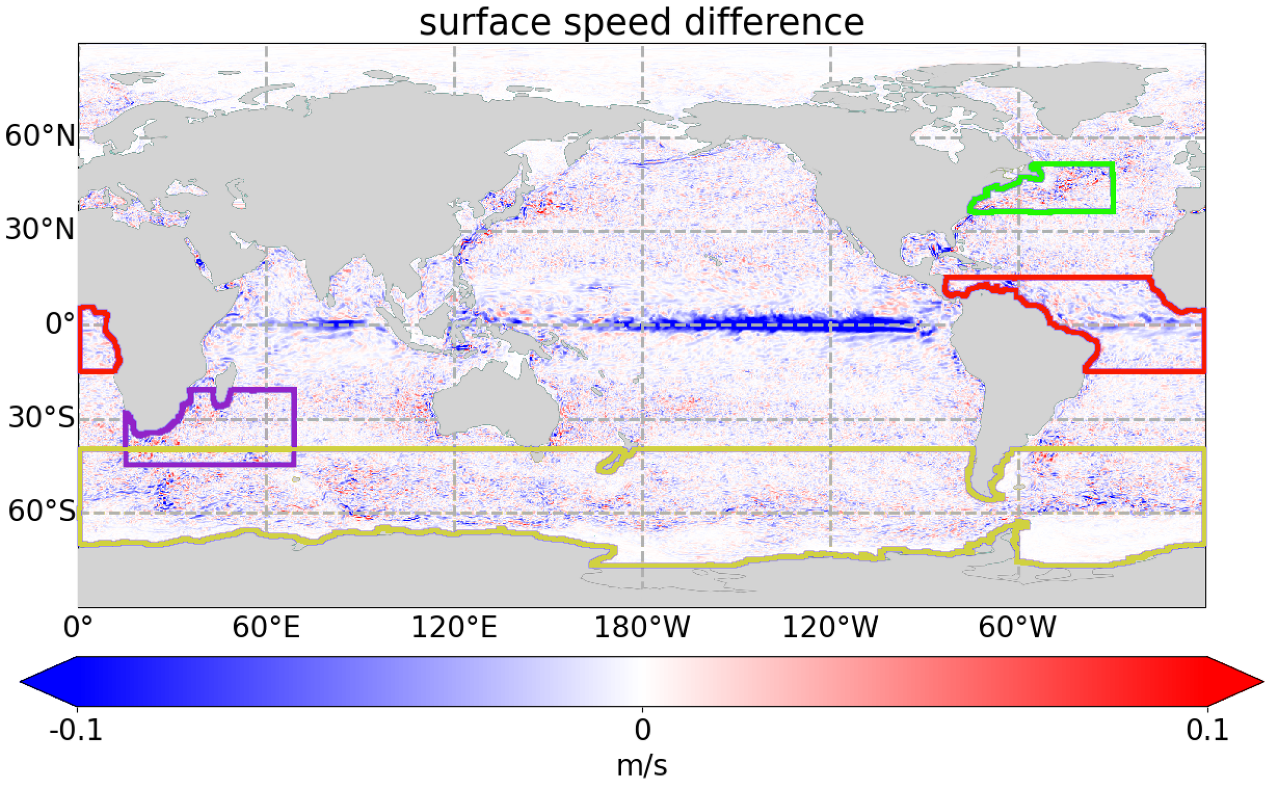
Spatial map of surface speed mean error difference between |A-TSCV Instr Err - NR| and |Control - NR| calculated from 25/02/2009 to 29/12/2009. The blue and red areas indicate that A-TSCV Instr Err or Control, respectively, is closer to NR. The boxes represent the regions of interest: Tropical Atlantic (red), Gulf Stream (green), Aghulas (purple), and Southern Ocean (yellow).
In this section, we report on features seen during the assessment allowing us to suggest possible ways of improvement for the system. Therefore, the assessment focuses on regions (see Figure 5) presenting a specific interest in the dynamics of the surface currents: i) the Tropical Atlantic (red area) for its wind-driven currents; ii) the Gulf Stream (green area) and the Agulhas Current (purple area) as geostrophic Western Boundary Currents (WBCs); iii) and the Antarctic Circumpolar Current (ACC; yellow area) for its barotropic nature.
4.1 Velocity improvement
The velocity RMSE is nicely improved globally at the surface. Even if this is partly due to an overfitting to the TSCV observations, the improvement is still genuine.
4.1.1 Tropical Atlantic
Figure 6 shows the surface velocity mean modeled by the NR for July (Figure 6A). Driven by the trade winds, the South Equatorial Current flows westward in two strong branches in July. The southern branch reaches the Brazilian coast where it carries on along the Northern coast as the North Brazil Current, the Guiana Current, and feeds eventually the Caribbean system. Note that a strong Ekman transport yields a northward current around 60°W. The northern branch retroflects to feed the eastward North Equatorial Counter Current which reaches the African coast and sustains a strong Guinea Current. The surface speed difference with respect to the NR is shown on Figures 6C, E for Control and A-TSCV Instr Err, respectively. We can clearly see that assimilating TSCV data helps reducing the mismatch to the NR for all the currents. Some discrepancy can still be seen in the North Brazil Current around the Amazon outflow, and at 60°W possibly due to an inaccurate Ekman transport. In November (Figure 6B), the South Equatorial Current is weaker. The North Brazil Current feeds the North Equatorial Counter Current that decreases rapidly. It also generates some large rings traveling along the coast as well as eastwards. Again, assimilating TSCV data (Figure 6F) reduces the mean error for all currents compared to the Control (Figure 6D). Apart from the North Brazil Current, the remaining discrepancies are located along the North Equatorial Counter Current although features like the double ring between 30°W and 40°W North of the Equator are well represented. The Hovmöller plots of Figure 7 show the RMSE difference between A-TSCV Instr Err and Control, with respect to NR. Assimilating the TSCV data is clearly beneficial in the upper 100 m (blue area). Around this depth however, the core of the strong Equatorial Undercurrent flows eastward. During the boreal spring, the improvement brought by the TSCV data can be seen down to 350 m. This corresponds to a period when the transport of the Equatorial Undercurrent is minimum. According to Brandt et al. (2014), 2009 was an anomalous year with a particularly weak transport at that time. For the rest of the year, the velocity RMSE is higher than the Control from 100 m depth. This could be due to the vertical projection of the surface velocity correction conflicting with the position and direction of the Equatorial Undercurrent.
Figure 6

Surface speed monthly mean in the Tropical Atlantic modelled by the NR in July (A) and November (B). Surface speed mean difference between Control and NR in July (C) and November (D). Surface speed mean difference between A-TSCV Instr Err and NR in July (E) and November (F).
Figure 7

Hovmöller of the RMSE difference between |A-TSCV Instr Err - NR| and |Control - NR| for zonal (A) and meridional (B) velocity in the first 500 m of Tropical Atlantic. The blue and red areas indicate that A-TSCV Instr Err or Control, respectively, is closer to NR.
4.1.2 Western boundary currents
The Gulf Stream carries warm water from the Tropics toward the north at the western part of the North Atlantic basin on about the first 1000 m of the water column. Figure 8 shows the Hovmöller plots of the velocity RMSE difference between A-TSCV Instr Err and Control, with respect to NR. The corrections brought by the TSCV data assimilation extend to depth, which is consistent with the Gulf Stream depth. A seasonal pattern can be seen with a degradation during fall, more pronounced at depth. This corresponds to the minimum transport of the seasonal variation of the Gulf Stream at depth. Focusing at 500 m depth, zonal (Figure 9A) and meridional (Figure 9B) velocities RMSE are decreased along the jet of the Gulf Stream in May whereas the results are more mixed in September.
Figure 8

Hovmöller of the RMSE difference between |A-TSCV Instr Err - NR| and |Control - NR| for zonal (A) and meridional (B) velocity in the first 1500 m of Gulf Stream. The blue and red areas indicate that A-TSCV Instr Err or Control, respectively, is closer to NR.
Figure 9

Spatial plot of the RMSE difference between |A-TSCV Instr Err - NR| and |Control - NR| for zonal (A) and meridional (B) velocity at 500 m in the Gulf Stream in May (top) and September (bottom). The blue and red areas indicate that A-TSCV Instr Err or Control, respectively, is closer to NR.
Along the eastern coast of South Africa, the Agulhas current flows southward regularly, before retroflecting when it encounters the ACC. Just below, at about 800 m, the deep Agulhas Undercurrent flows equatorward. Figure 10 shows the RMSE profiles of the region. Assimilating TSCV data improves slightly the statistics in the first 300 m, but degrades them below. Other western boundary currents have been studied and show the same kind of results.
Figure 10

RMSE profiles of the difference Control - NR (blue) and A-TSCV Instr Err - NR (orange) for zonal (A) and meridional (B) velocity in the Agulhas region, calculated from 25/02/2009 to 29/12/2009.
Compared to the Tropics, the improvement of the surface velocity RMSE is much smaller in the WBCs. This can be possibly explained by the numerous meanders and rings involving smallest scales. The forecast and analysis vectors are computed on a coarser horizontal grid of 1/2°. This resolution is barely able to capture meso-scale features.
4.1.3 Antarctic Circumpolar Current
In the Southern Ocean, the ACC flows continuously around Antarctica. The TSCV data are provided until 60°S, which covers partially the ACC. Figure 11 shows the profiles of zonal (Figure 11A) and meridional (Figure 11B) velocity for Control (blue) and A-TSCV Instr Err (orange) in the Southern Ocean. Assimilating TSCV data is beneficial along the whole water column, which is consistent with the barotropic nature of the flows. For both zonal and meridional velocities, the RMSE is reduced by 1 cm/s at surface (10% improvement) and is still reduced by a few mm/s at the bottom.
Figure 11

RMSE profile of the difference Control - NR (blue) and A-TSCV Instr Err - NR (orange) for zonal (A) and meridional (B) velocity in the Southern Ocean, calculated from 25/02/2009 to 09/06/2009.
4.1.4 Forecasts
Seven-day forecasts are launched every week at the start of an assimilation window. These forecasts are compared to the NR to evaluate how much of the correction is retained by the model. Figure 12 shows the mean and RMSE surface zonal velocity in the different regions. The benefit of assimilating TSCV data is preserved during the entire forecast. In the Tropical Atlantic, the RMSE of the 7th forecast day for A-TSCV Instr Err is still smaller than the RMSE of the 1st forecast day for Control. In the ACC, the gain is of about 2 days. The RMSE gain in the WBC regions is less than 1 day due to a poor improvement in the analysis. Results are similar for the surface meridional velocity.
Figure 12

7-day forecasts mean (dashed lines) and RMSE (plain lines) for surface zonal velocity for Control (blue) and A-TSCV Instr Err (orange) with respect to NR, in Tropical Atlantic (A), Gulf Stream (B), Agulhas (C) and ACC (D).
4.2 Deteriorations and possible solutions
While the velocity RMSE is improved at the surface and at depth to some extent depending on the region, it is degraded further down. Apart from the Tropics and the Southern Ocean where a small improvement can be spotted at surface and sub-surface, the temperature and salinity RMSEs are slightly degraded (see Figure 13 for temperature). The differences in salinity however, are very small. Regarding SSH, the improvement in RMSE is very small in all regions. This is disappointing, especially in the WBCs, where the geostrophy should lead to a more intense relationship between SSH and velocities. As shown on the example of the Gulf Stream of Figure 14B, improvements and degradations alternate, leading to this regional poor improvement. Interestingly however, a small improvement of about 2 mm can be seen along the Equator (see Figure 14A for Tropical Atlantic), suggesting that covariances include an ageostrophic relationship between the surface currents and SSH.
Figure 13

RMSE temperature profiles of the difference Control - NR (blue) and A-TSCV Instr Err - NR (orange) in the Tropical Atlantic (A) and the Gulf Stream (B) calculated from 25/02/2009 to 09/06/2009.
Figure 14
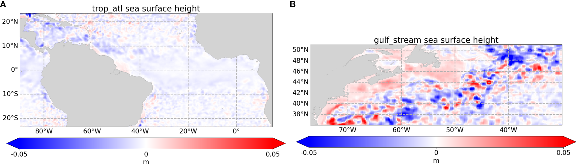
RMSE SSH spatial map of the RMSE difference between |A-TSCV Instr Err - NR| and |Control - NR| in Tropical Atlantic (A) and Gulf Stream region (B). The blue and red areas indicate that A-TSCV Instr Err or Control, respectively, is closer to NR.
As seen in Section 3.5, the vertical RMSE degradations are more or less strong depending on the TSCV observation thinning that is used. This suggests that the vertical projection of the correction brought by the surface data could not be completely appropriate. The vertical background error covariances are not limited in space in contrast to the horizontal covariances. Small univariate and multivariate contributions can therefore act as spurious correlations deteriorating the statistics. A filtering could hence be performed on the background error correlations to set to zero any correlations below a defined threshold. But small contributions are not necessarily spurious and this method might cause a loss of improvement in some regions. A vertical limit could also be applied, depending on some dynamical features. For example, the mixed layer depth could be used to split the stratified waters from the rest of the water column (Waters et al., 2015).
The background error variances are adjusted by computing a coefficient according to the Desroziers innovation diagnostics. However, the observations used to establish the diagnostics are limited to SST and SSH observations. The current networks for these observations allow for a global coverage and their number is dominant in the background error covariance matrix trace when classical observations only are assimilated. When TSCV data are assimilated as well, this is no longer true, and a possible discrepancy can occur, yielding RMSE degradations. Innovations associated with the TSCV data should therefore be accounted for in the diagnostics. However, one should be careful to ensure that their number will not dominate the trace.
The background error structure is calculated from the statistics of anomalies extracted from a long run where only large scale temperature and salinity are corrected by data assimilation. This structure is hence climatological and can sometimes misplace features such as fronts, rings or eddies. It could therefore be beneficial to complement this static structure with a more dynamic structure representing the current situation. This is basically the idea behind ensemble data assimilation. In our case, a possibility could be to associate a structure of the week calculated from anomalies of the 7-day forecast used to calculate the innovations.
To save computing time, the forecast and analysis vectors are computed on a coarser grid at an horizontal resolution of 1/2°. In dynamical regions such as the WBCs, this resolution could be detrimental. To alleviate such issues, the coarser grid could be redefined by eliminating more points in calm regions such as the gyres, and keeping the higher resolution in high variability regions. Sequential analyses accounting for specific ranges of scales could also help resolving these issues.
5 Summary and discussion
The MOI assimilation system has been monitoring and forecasting ocean and sea ice variables for more than twenty years in global and regional configurations. Although the velocities are not constrained by current observations, they are predicted with a satisfying accuracy even if their magnitude is generally underestimated. To answer the challenge of predicting more accurate velocities, OSSEs have been run in the framework of the A-TSCV project to assess the impact of assimilating satellite TSCV data. The TSCV is the sum of different current contributions including the geostrophic and wind-driven currents, the Stokes drift, the tidal signal and the near-inertial oscillations.
For the OSSEs, temperature and salinity vertical profiles, SST maps, SSH and TSCV data are extracted from the NR, a global 1/12° simulation without any data assimilation. Because there is no coupling with wave and tide models in the NR, the TSCV data does not include any Stokes drift nor tidal signal. The OSSEs consist of a Control experiment that assimilates the simulated classical observations but not the TSCV data, and different A-TSCV experiments that assimilate both classical and TSCV observations. The configuration of these experiments is chosen such that it will introduce differences with the NR (model versions, horizontal resolution, atmospheric forcing) so that their statistics are comparable to those of the operational system. An experiment without any assimilation is also run and shows that these differences are significant enough.
A sensitivity analysis has been performed by comparing different TSCV observation density (one over two or one over sixteen observations) and different prescribed observation errors (with or without instrument error). The results of the experiments show that high observation density leads to an overfitting to the TSCV data at the surface. This overfitting is projected vertically by the background error covariances and yields velocity RMSE degradations at depth. Having a higher prescribed observation error (with instrument error) limits these degradations. The lower density observation network associated with the higher prescribed observation error leads to a smaller improvement in the velocity RMSE at the surface (no overfitting) but generally eliminates the degradations at depth.
The assessment is performed in terms of mean and RMSE of the differences between the experiments and the NR. The statistics of the Control and the A-TSCV Instr Err (one over two TSCV observations, prescribed observation error including instrument error) are compared in regions of interest: Tropical Atlantic, Gulf Stream, Agulhas Current and ACC. The global assessment is reported in Waters et al. (2024b). At the surface and down to some depth, assimilating TSCV data reduces the velocity RMSE. This is particularly true in the Tropics. A part of this improvement however, is due to an overfitting to the TSCV data. At depth, the RMSE degradation varies seasonally depending on the dynamics of the currents. Temperature and salinity RMSEs are generally slightly degraded except in the Tropics where they are improved at the surface and sub-surface. SSH results are mixed, often alternating spatial improvements and degradations.
The RMSE degradations have been analyzed and some possible solutions have been provided. They mainly consist at reworking the background error covariances to eliminate possible spurious vertical correlations, and adjust the variances by accounting for the TSCV observations. The current covariances being static, covariances calculated for each assimilation window could lead to improvements. Eventually, the analysis grid could be redefined to preserve the highest resolution in regions with high variability, or sequential analyses for specific ranges of scales could be performed.
In the experiments, the TSCV data is assimilated through its zonal and meridional components as independent variables. This is not ideal but eases the complexity of the observation operator and the covariances to apply. Other ways could be tried such as assimilating speed and angles, stream functions, or current divergence and rotational components.
The OSSEs reported in this paper constitute a first attempt at assimilating satellite surface velocities in the MOI analysis and forecasting system. Apart from a new observation operator, no specific tuning has been done, in order to be able to evaluate the current configuration and setup. This gave us insights on the impact of such data and about aspects of the system that could be improved to make a better use of this data. A next step could be to try and implement some of the suggestions listed above and analyze their effect.
Statements
Data availability statement
The raw data supporting the conclusions of this article will be made available by the authors, without undue reservation.
Author contributions
IM: Formal analysis, Investigation, Methodology, Validation, Visualization, Writing – original draft, Writing – review & editing. ER: Formal analysis, Methodology, Writing – review & editing. J-ML: Methodology, Writing – review & editing. MM: Methodology, Project administration, Writing – review & editing. CD: Funding acquisition, Project administration, Writing – review & editing.
Funding
The author(s) declare financial support was received for the research, authorship, and/or publication of this article. The A-TSCV project, namely Assimilation of Total Surface Current Velocity Measurements (A-TSCV), received funding from the European Space Agency under grant agreement No. 4000130863/20/NL/IA.
Acknowledgments
The authors would like to thank Lucile Gaultier and Clément Ubelmann for providing the SSH and TSCV simulated observations, and Florent Gasparin for providing the simulated in situ and SST observations. They also would like to thank Jennifer Waters for leading the work package about the implementation of the OSSEs and for the useful discussions. The main author is grateful to the Mercator Ocean International team for its help at handling the MOI system.
Conflict of interest
The authors declare that the research was conducted in the absence of any commercial or financial relationships that could be construed as a potential conflict of interest.
Publisher’s note
All claims expressed in this article are solely those of the authors and do not necessarily represent those of their affiliated organizations, or those of the publisher, the editors and the reviewers. Any product that may be evaluated in this article, or claim that may be made by its manufacturer, is not guaranteed or endorsed by the publisher.
References
1
Aijaz S. Brassington G. B. Divakaran P. Regnie C. Drevillon M. Maksymczuk J. et al . (2023). Verification and intercomparison of global ocean eulerian near-surface currents. Ocean Model.186. doi: 10.1016/j.ocemod.2023.102241
2
Ardhuin F. Chapron B. Maes C. Romeiser R. Gommenginger C. Cravatte S. et al . (2019). Satellite doppler observations for the motions of the oceans. Bull. Am. Meteorol. Soc100, ES215–ES219. doi: 10.1175/BAMS-D-19-0039.1
3
Ardhuin F. Marie L. Rascle N. Forget P. Roland A. (2009). Observation and estimation of lagrangian, stokes, and eulerian currents induced by wind and waves at the sea surface. J. Phys. Oceanogr.39, 2820–2838. doi: 10.1175/2009JPO4169.1
4
Benkiran M. Ruggiero G. Greiner E. Le Traon P.-Y. Remy E. Lellouche J.-M. et al . (2021). Assessing the impact of the assimilation of swot observations in a global high-resolution analysis and 567 forecasting system part 1: Mathods. Front. Mar. Sci.8. doi: 10.3389/fmars.2021.691955
5
Bidlot J.-R. (2012). Impact of ocean surface currents on the ecmwf forecasting system for atmosphere circulation and ocean waves. In GlobCurrent Preliminary User Consultation Meeting.
6
Bloom S. C. Takacs L. L. Da Silva A. M. Ledvina D. (1996). Data assimilation using incremental 571 analysis updates. Mon. Weather Rev.124, 1256–1271. doi: 10.1175/1520-0493(1996)124<1256:DAUIAU>2.0.CO;2
7
Brandt P. Funk A. Tantet A. Johns W. E. Fischer J. (2014). The equatorial undercurrent in the central atlantic and its relation to tropical atlantic variability. Clim. Dynam.43, 2985–2997. doi: 10.1007/s00382-014-2061-4
8
Brasseur P. Verron J. (2006). The seek filter method for data assimilation in oceanography: a synthesis. Ocean Dynam.56, 650–661. doi: 10.1007/s10236-006-0080-3
9
Chassignet E. P. Xu X. (2017). Impact of horizontal resolution (1/12° to 1/50°) on gulf stream separation, penetration and variability. J. Phys. Oceanogr.47, 1999–2021. doi: 10.1175/JPO-D-17-0031.1
10
Desroziers G. Berre L. Chapnik B. Poli P. (2005). Diagnosis of observation, background and analysis-errror statistics in observation space. Q. J. R. Meteorol. Soc131, 3385–3396. doi: 10.1256/qj.05.108
11
Drevillon M. Greiner E. Paradis D. Payan C. Lellouche J.-M. Reffray G. et al . (2013). A strategy for producing refined currents in the equatorial atlantic in the context of the search of the af447 wreckage. Ocean Dynam.63, 63–82. doi: 10.1007/s10236-012-0580-2
12
Du Y. Dong X. Jiang X. Zhang Y. Zhu D. Sun Q. et al . (2021). Ocean surface current multiscale observation mission (oscom): Simultaneous measurement of ocean surface current, vector wind, and temperature. Prog. Oceanography193, 102531. doi: 10.1016/j.pocean.2021.102531
13
Duan B. Zhang W. Dai H. (2018). Ascat wind superobbing based on feature box. Advances Meteorology2018. doi: 10.1155/2018/3438501
14
Fichefet T. Morales Maqueda M. A. (1997). Sensitivity of a global sea ice model to the treatment of ice thermodynamics and dynamics. J. Geophys. Res.102, 12609–12646. doi: 10.1029/97JC00480
15
Gasparin F. Greiner E. Lellouche J.-M. Legalloudec O. Garric G. Drillet Y. et al . (2018). A large-scale view of oceanic variability from 2007 to 2015 in the global high resolution monitoring and forecasting system at mercator ocean.´. J. Mar. Syst.187, 260–276. doi: 10.1016/j.jmarsys.2018.06.015
16
Gasparin F. Guinehut S. Mao C. Mirouze I. Remy E. King R. R. et al . (2019). Requirements for an integrated in situ atlantic ocean observing system from coordinated observing system simulation experiments. Front. Mar. Sci.6. doi: 10.3389/fmars.2019.00083
17
Gaultier L. Ubelmann C. (2022). SKIMulator A-TSCV Simulation: System description, configuration and simulations. Report ESA A-TSCV TR-3.
18
Gaultier L. Ubelmann C. Fu L.-L. (2016). The challenge of using future swot data for oceanic field reconstruction. J. Atmos. Ocean. Tech.33, 119–126. doi: 10.1175/JTECH-D-15-0160.1
19
Gommenginger C. Chapron B. Hogg A. Buckingham C. Fox-Kemper B. Eriksson L. et al . (2019). Seastar: A mission to study ocean submesoscale dynamics and small-scale atmosphere-ocean processes 603 in coastal, shelf and polar seas. Front. Mar. Sci.6. doi: 10.3389/fmars.2019.00457
20
Hersbach H. Bell B. Berrisford P. Hirahara S. Horanyi A. Munoz-Sabater J. et al . (2020). The era5 global reanalysis. Q. J. R. Meteorological Soc.146, 1999–2049. doi: 10.1002/qj.3803
21
Hoffman R. N. Atlas R. (2016). Future observing system simulation experiments. Bull. Am. Meteorol. Soc.97, 1601–1616. doi: 10.1175/BAMS-D-15-00200.1
22
Huang B. Wang X. (2018). On the use of cost-effective valid-time-shifting (vts) method to increase 609 ensemble size in the gfs hybrid 4denvar system. Mon. Weather Rev.146, 2973–2998. doi: 10.1175/MWR-D-18-0009.1
23
Isern-Fontanet J. Ballabrera-Poy J. Turiel A. Garcia-Ladona E. (2017). Remote sensing of ocean surface currents: a review of what is being observed and what is being assimilated. Nonlinear Proc. Geoph.24, 613–643. doi: 10.5194/npg-24-613-2017
24
Janjic T. Bormann N. Bocquet M. Carton J. A. Cohn S. E. Dance S. L. et al . (2018). On the representation error in data assimilation. Q. J. R. Meteorolog. Soc144, 1257–1278. doi: 10.1002/qj.3130
25
Krug M. Mouche A. Collard F. Hohannessen J. A. Chapron B. (2010). Mapping the agulhas current from space: an assessment of asar surface current velocities. J. Geophys. Res.115, C10026. doi: 10.1029/2009JC006050
26
Large W. G. Yeager S. G. (2009). The global climatology of an interannually varying air-sea flux data set. Clim. Dynam.33, 341–364. doi: 10.1007/s00382-008-0441-3
27
Laxague N. J. M. Ozgokmen T. M. Haus B. K. Novelli G. Shcherbina A. Sutherland P. et al . (2017). Observations of near-surface current shear help describe oceanic oil and plastic transport. Geophys. Res. Lett.45, 245–249. doi: 10.1002/2017GL075891
28
Lellouche J.-M. Greiner E. Le Galloudec O. Garric G. Regnier C. Drevillon M. et al . (2018). Recent updates to the copernicus marine service global ocean monitoring and forecasting real-time 1/12° high-resolution system. Ocean Sci.14, 1093–1126. doi: 10.5194/os-14-1093-2018
29
Lellouche J.-M. Le Galloudec O. Drevillon M. Regnier C. Greiner E. Garric G. et al . (2013). Evaluation of global monitoring and forecasting systems at mercator ocean.´. Ocean Sci.9, 57–81. doi: 10.5194/os-9-57-2013
30
Liu X. Weinbren A. L. Chang H. Tadic J. M. Mountain M. E. Trudeau M. E. et al . (2021). Data reduction for inverse modeling: an adaptive approach v1.0. Geoscientific Model. Dev.14, 4683–4696. doi: 10.5194/gmd-14-4683-2021
31
Lopez-Dekker P. Rott H. Prts-Iraola P. Chapron B. Scipal K. De Witte E. (2019). “Harmony: an earth explorer 10 mission candidate to observe land, ice and ocean surface dynamics,” in IGARSS 2019 (2019 IEEE International Geoscience and Remote Sensing Symposium, Yokohama, Japan), 8381–8384. doi: 10.1109/IGARSS40859.2019
32
Lumpkin R. Ozgokmen T. Centurioni L. (2017). Advances in the application of surface drifters. Annu. Rev. Mar. Sci.9, 59–81. doi: 10.1146/annurev-marine-010816-060641
33
Madec G. (2008). NEMO ocean engine (Institut Pierre-Simon Laplace, Paris: Tech. Rep. Note du Pole de modelisation´ No 27 ISSN No 1288-1619).
34
Madec G. Bourdalle-Badie R. Bouttier P.-A. Bricaud C. Bruciaferri D. Calvert D. et al . (2017). NEMO ocean engine (Version v3.6). Notes du Poleˆ de Modelisation´ de l’Institut Pierre-Simon Laplace (IPSL) (Tech. rep., Institut Pierre-Simon Laplace (IPSL). doi: 10.5281/zenodo.1472492
35
Madec G. Imbard M. (1996). A global ocean mesh to overcome the north pole singularity. Clim. Dynam.12, 381–388. doi: 10.1007/BF00211684
36
Marie L. Collard F. Nouguier F. Pineau-Guillou L. Hauser D. Boy F. et al . (2020). Measuring ocean total surface current velocity with the kuros and karadoc airborne near-nadir doppler radars: a multi-scale analysis in preparation for the skim mission. Ocean Sci.16, 1399–1429. doi: 10.5194/os-16-1399-2020
37
Ochotta T. Gebhardt C. Saupe D. Wergen W. (2005). Adaptive thinning of atmospheric observations in data assimilation with vector quantization and filtering methods. Q. J. R. Meteorolog. Soc131, 3427–3437. doi: 10.1256/qj.05.94
38
Pham D. T. Verron J. Roubaud C. (1998). A singular evolutive extended Kalman filter for data assimilation in oceanography. J. Mar. Sys.16, 323–340. doi: 10.1016/S0924-7963(97)00109-7
39
Purser R. J. Wu W. S. Parrish D. F. Roberts N. M. (2003). Numerical aspects of the application of recursive filters to variational statistical analysis. part I: Spatially homogeneous and isotropic Gaussian covariances. Mon. Weather Rev.131, 1524–1535. doi: 10.1175//1520-0493(2003)131<1524:NAOTAO>2.0.CO;2
40
Renault L. McWilliams J. C. Masson S. (2017). Satellite observations of imprint of oceanic current on wind stress by air-sea coupling. Sci. Rep.7, 17747. doi: 10.1038/s41598-017-17939-1
41
Rohrs J. Sutherland G. Jeans G. Bedington M. Sperrevik A. K. Dagestad K.-F. et al . (2021). Surface currents in operational oceanography: Key applications, mechanisms, and methods. J. Oper. Oceanogr.16, 60–88. doi: 10.1080/1755876X.2021.1903221
42
Rubio A. Mader J. Corgnati L. Mantovani C. Griffa A. Novellino A. et al . (2017). Hf radar activity in european coastal seas: next steps toward a pan-european hf radar network. Front. Mar. Sci.4. doi: 10.3389/fmars.2017.00008
43
Sandery P. A. Sakov P. (2017). Ocean forecasting of mesoscale features can deteriorate by increasing model resolution towards the submesoscale. Nat. Commun.8, 1566. doi: 10.1038/s41467-017-01595-0
44
Torres H. Wineteer A. Klein P. Lee T. Wang J. Rodriguez E. et al . (2023). Anticipated capabilities of the odysea wind and current mission concept to estimate wind work at the air-sea interface. Remote Sens.15, 3337. doi: 10.3390/rs15133337
45
Vancoppenolle M. Fichefet T. Goose H. Bouillon S. Madec G. Morales Maqueda M. A. (2009). Simulating the mass balance and salinity of arctic and antarctic sea ice. 1. model description and 668 validation. Ocean Model.27, 33–53. doi: 10.1016/j.ocemod.2008.10.005
46
Waters J. Martin M. J. Bell M. M. King R. R. Gaultier L. Ubelmann C. et al . (2024a). Assessing the potential impact of assimilating total surface current velocities in the met office’s global ocean 671 forecasting system. Front. Mar. Sci. doi: 10.3389/fmars.2024.1383522
47
Waters J. Martin M. J. Lea D. J. Mirouze I. Weaver A. T. While J. (2015). Implementing a variational data assimilation system in an operational 1/4 degree global ocean model. Q. J. R. Meteorol. Soc141, 333–349. doi: 10.1002/qj.2388
48
Waters J. Martin M. J. Mirouze I. Remy E. King R. R. Gaultier L. et al (2024b). The impact of simulated total surface current velocity observations on operational ocean forecasting and requirements for future satellite missions. Front. Mar. Sci.11, 1408495. doi: 10.3389/fmars.2024.1408495
49
Yu L. Fennel K. Wang B. Laurent A. Thompson K. R. Shay L. K. (2019). Evaluation of nonidentical versus identical twin approaches for observation impact assessments: an ensemble-kalman-filter-based ocean assimilation application for the gulf of Mexico. Ocean Sci.15, 1801–1814. doi: 10.5194/os-15-1801-2019
Summary
Keywords
ocean currents, SKIM, OSSE, background error covariance, ocean forecast
Citation
Mirouze I, Rémy E, Lellouche J-M, Martin MJ and Donlon CJ (2024) Impact of assimilating satellite surface velocity observations in the Mercator Ocean International analysis and forecasting global 1/4° system. Front. Mar. Sci. 11:1376999. doi: 10.3389/fmars.2024.1376999
Received
26 January 2024
Accepted
08 May 2024
Published
12 June 2024
Volume
11 - 2024
Edited by
Gilles Reverdin, Centre National de la Recherche Scientifique (CNRS), France
Reviewed by
Rick Lumpkin, Atlantic Oceanographic and Meteorological Laboratory (NOAA), United States
Nikki Prive, Morgan State University, United States
Updates
Copyright
© 2024 Mirouze, Rémy, Lellouche, Martin and Donlon.
This is an open-access article distributed under the terms of the Creative Commons Attribution License (CC BY). The use, distribution or reproduction in other forums is permitted, provided the original author(s) and the copyright owner(s) are credited and that the original publication in this journal is cited, in accordance with accepted academic practice. No use, distribution or reproduction is permitted which does not comply with these terms.
*Correspondence: Isabelle Mirouze, imirouze@mercator-ocean.fr
Disclaimer
All claims expressed in this article are solely those of the authors and do not necessarily represent those of their affiliated organizations, or those of the publisher, the editors and the reviewers. Any product that may be evaluated in this article or claim that may be made by its manufacturer is not guaranteed or endorsed by the publisher.