 Linghan Meng1,2
 Haibin Song
94% of researchers rate our articles as excellent or good
Learn more about the work of our research integrity team to safeguard the quality of each article we publish.
Find out more
ORIGINAL RESEARCH article
Front. Mar. Sci., 09 July 2024
Sec. Ocean Observation
Volume 11 - 2024 | https://doi.org/10.3389/fmars.2024.1376945
Seismic oceanography has been widely used in the study of internal solitary waves (ISWs) in recent years, and has achieved remarkable results. In this paper, we analyzed the multi-channel seismic reflection data in the Canterbury Basin offshore New Zealand from January 9 to January 29, 2000, collected by R/V Maurice Ewing. We observed 4 groups of ISWs (labeled ISW1s to ISW4s) on 4 seismic survey lines. We studied their waveforms and propagation speeds in detail. There are two theoretical structures used to describe the vertical waveform of ISWs: the first-order nonlinear vertical structure and the linear vertical structure. We found that ISW1s fit the nonlinear structure well, ISW3s and ISW4s fit the linear structure, and ISW2 does not fit either one. As the water depth increases, the waveforms of all ISWs gradually widen. Two satellite SAR images reveal that all ISWs generally travel shoreward across the isobaths. However, the propagation direction of ISW1s is about 354°-360° (clockwise from due north), different from the propagation directions of other ISWs (about 22°-26°), which explains why ISW1s have the largest characteristic half-height width. The estimated propagation speeds are close to the theoretical speeds, confirming our speed correction method. In the end, we also discuss the interaction of ISWs and eddies.
Internal solitary waves (ISWs) are special internal waves in the ocean with characteristics of nonsinusoidal, nonlinear, large-amplitude, and isolated waveforms. They can be generated by direct excitation in the stratified ocean or by nonlinear evolution in the internal tide propagation (Maxworthy, 1979; Apel et al., 1985; Apel, 1987; Ostrovsky and Stepanyants, 1989; Ramp et al., 2004). ISWs can induce large isopycnal displacements and strong currents, which affect the transfer of ocean kinetic energy and vertical mixing (Munk and Wunsch, 1998; Wunsch, 2004), the transport of sediment and shaping of seabed sedimentary landforms (Geng et al., 2018; Boegman and Stastna, 2019), and threaten offshore construction and engineering, such as drilling platforms, submarine cables, and oil pipelines (Cai et al., 2015).
Nonlinearity and non-hydrostatic dispersion play a critical role in the generation and propagation of ISWs. Nonlinearity tends to steepen the waveforms of ISWs, while dispersion makes them wider. Under the equilibrium of these two effects, ISWs can keep their waveforms and travel far in the ocean. When ISWs move from deep into shallow water, their waveforms gradually change because of the imbalances between nonlinear and dispersion; the slope of their leading edges decreases with increasing wavelength, while the slope of their back edges gets steeper. On the trailing edge, it also makes short-wavelength oscillatory waves (Orr and Mignerey, 2003). During the shoaling process, Kelvin-Helmholtz instability or convective instability may happen (Duda et al., 2004; Lien et al., 2012). Sometimes an ISW grows into a well-organized wave packet (Liao et al., 2014). However, the detailed process is still under intensive research, which is mainly hampered by the lack of high-resolution in-situ observations.
Almost all ocean instruments that measure current, temperature, or other parameters can show the presence of ISWs and can be used to study ISWs. Satellite remote sensing and high-frequency echo sounding are often used. The former detects the surface signatures of ISWs and obtains information such as generation source, spatial distribution, waveform characteristics (wavelength, crest length, wave spacing), and propagation speed. It mainly consists of Synthetic Aperture Radar (SAR) and optical MODIS images (Liu et al., 1998; Jackson, 2007). The high-frequency echo sounding is a backscattering system and can take a picture of the vertical 2D structure of ISWs (Farmer and Armi, 1999; Orr and Mignerey, 2003; Klymak and Gregg, 2004; Reeder et al., 2011; Bai et al., 2019; Feng et al., 2021). However, its application is mainly limited by its shallow investigation depth and difficulty in extracting quantitative information (Tang et al., 2015).
Seismic oceanography (Holbrook, 2003) is a new technique that studies physical ocean phenomena using conventional low-frequency marine seismic reflection. Thanks to the advantages of fast acquisition speed, high horizontal resolution, and full-depth seawater column imaging, seismic oceanography has been widely used in the study of internal waves (Holbrook and Fer, 2005), internal solitary waves (Tang et al., 2014, Tang et al, 2015, Tang et al, 2016; Bai et al., 2017; Buffett et al., 2017; Tang et al., 2018; Geng et al., 2019; Fan et al., 2021; Gong et al., 2021a, Gong et al, 2021a; Song et al., 2021a; Song et al., 2021b; Wei et al., 2022), and eddies (Song et al., 2011; Yang et al., 2022; Zhang et al., 2022). In this paper, we will study ISWs offshore the South Island of New Zealand, where abundant seismic data coincide with a significant oceanographic setting. Also, ISWs have an important impact on local fisheries and marine oil engineering. However, there are few reports about ISWs in this region (Cooper et al., 2021). The original multichannel seismic data acquired in this area has been reprocessed. Several ISWs are observed, and their vertical structures, lateral structures, and propagation speeds are studied.
The rest of this paper is arranged as follows: Section 2 introduces data and methods, including seismic data acquisition and processing, hydrographic information, and the theoretical model of ISWs. The research results are given in Section 3. We study the vertical structural characteristics of ISWs and compare them with two theoretical models. Then, the KdV (Korteweg-de Vries) equation and seismic data are used to calculate the theoretical phase speed, the observed speed, and the related parameters of ISWs. Finally, the lateral structures of ISWs are studied. In Section 4, we discuss the effects of topography, water depth, and amplitude on propagation speed. Data from hydrologic reanalysis and seismic data are also used to study the interaction between ISWs and eddies. Section 5 is a summary.
From January 9 to January 29, 2000 (cruise EW0001), R/V Maurice Ewing collected high-resolution multi-channel seismic reflection data at the shelf and slope of New Zealand’s offshore Canterbury Basin. 84 multi-channel seismic survey lines were acquired during this cruise. The acoustic source consisted of two 45/45 cubic inch GI air guns (pressure 2000 psi), sunk at 2.5 to 3.5 m, and fired every 5 s. The average cruise speed of the ship was about 2.5 m/s during acquisition, which means the source fired at a distance of about 12.5 m. The data were recorded by a cable of 96 or 120 channel hydrophones at a channel space of 12.5 m. The recording time was 3 s, with a sampling time of 1 ms.
Seismic Unix can be used to reprocess the original seismic data to get a seismic oceanography section and make a snapshot of the thermohaline structure of the seawater column at full depth. The main processes include trace editing, the definition of the observation system, de-noising (removal of low-frequency noise and suppression of direct waves), common midpoint gathers (CMPs) sorting, speed analysis, normal move-out (NMO) correction, stacking, and post-stack de-noising. For the convenience of follow-up processing, we usually reconstruct the observation system in the cartesian coordinate system. A high-pass filter suppresses low-frequency noise, such as swell waves below 8 Hz. The near-offset direct waves can directly cover the reflected signals, especially in the shallow water layer. The shallow water is the area with the most abundant physical oceanographic phenomena, so it cannot be directly muted. Therefore, we use the median filtering and matching subtraction method to suppress them effectively. Next, we sort the seismic traces into CMPs, conduct speed analysis and NMO correction, and finally stack the processed CMPs. In post-stack processing, dip-angle filtering is used to further suppress the noise and get a clear reflection seismic image (e.g., Ruddick et al, 2009).
We used the HYCOM (Hybrid Coordinate Ocean Model) reanalysis product and historical CTD data to study the currents and water mass characteristics offshore the South Island of New Zealand (Figure 1). The HYCOM reanalysis is a product developed by the United States Naval Research Laboratory, which has assimilated multi-source observational data using the Navy Coupled Ocean Data Assimilation (NCODA) system. In this paper, we use the hydrography data generated from January 1 to January 30, 2000, by HYCOM. The horizontal resolution of the HYCOM data is 1/12°, and the vertical resolution is 40 layers from 0 to 5000 m.
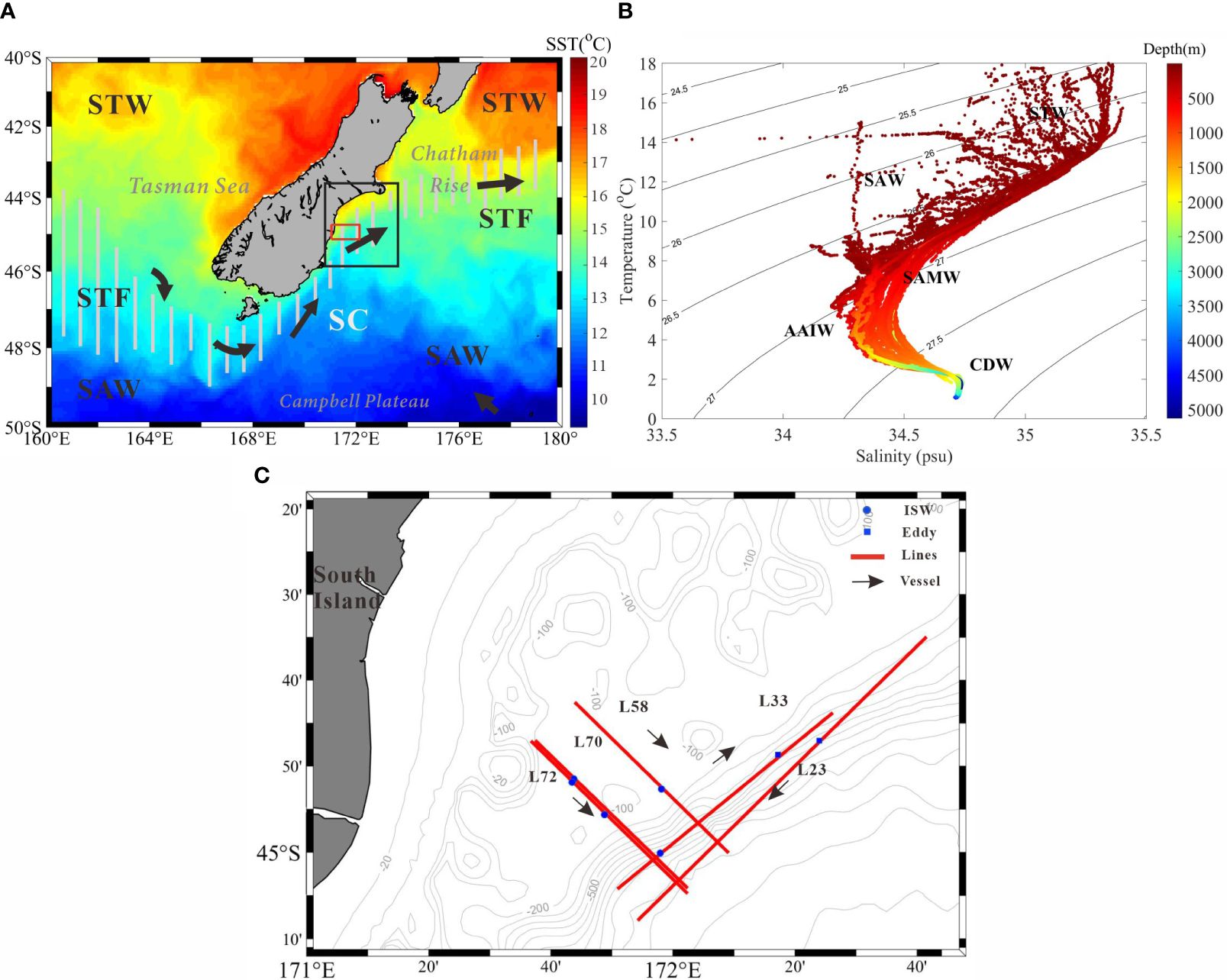
Figure 1 (A) Geographical and oceanographic characteristics offshore South Island, New Zealand (after Gorman et al., 2018). The vertical gray bar shows the location of front zone, the arrows represent currents, and the background colors indicate sea surface temperature. The red rectangle shows the region of seismic survey. The black rectangle represents the region of SAR images (Figure 8). STW, Subtropical Water; STF, Subtropical Front; SAW, Subantarctic Water; SC, Southland Current. (B) Temperature-salinity (T-S) diagram of the study area. (C) Locations of seismic lines L33, L58, L70, and L72 (solid red lines), blue dots represent the position of ISWs, blue squares represent the position of eddies, and arrows represent the direction of the survey ship.
Water masses offshore the South Island of New Zealand can be classified into surface water mass, subsurface water mass, intermediate water mass, and deep water mass. The surface water mass is subtropical water (STW), which is warm and salty. It is located in the Tasman Sea to the west of New Zealand and to the north of the Chatham Rise on the east coast of New Zealand. The subantarctic water (SAW) is slightly cooler and less salty than STW and covers most of the offshore area, south and east of the South Island, and south of the Chatham Rise. The subtropical front (STF) separates the two surface water masses to the north and south (Neil et al., 2004; Chiswell et al., 2015). The subantarctic mode water (SAMW) is a water mass below the surface that has a temperature of 7-9 °C and a salinity of 34.35-34.5 psu. The salinity minimum around the South Island is known as Antarctic intermediate water (AAIW), which centers at 700-1000 m. The Circumpolar Deep Water (CDW) is 1400-3500 m deep. The Southland Current (SC) flows south along the southwest coast of the South Island, then east through the Foveaux Strait, and finally north along the east coast of the South Island (Cooper et al., 2021).
In recent years, with the advent of advanced marine instruments, we have had more and more opportunities to observe and study ISWs in the ocean. In the research process, it is usually necessary to use the relevant theoretical model to obtain the theoretical waveform curve. Among them, the KdV equation is a classic model for studying the structure of weak nonlinear ISWs. In the absence of background flow and frictional dissipation, the KdV equation can be expressed as (Djordjevic and Redekopp, 1978; Ostrovsky and Stepanyants, 1989):
where t is the time and x is the distance along the propagation direction. Under the condition of Boussinesq approximation, is used to describe the evolution of the waveform with time when the wave travels along the x direction. c is the linear phase speed, α and β represent the quadratic nonlinear coefficient and dispersion coefficient, respectively, which can be obtained by the following formula:
and
where H represents the water depth, ϕ the vertical structure function. For the continuous stratification model, these parameters can be calculated by the formula:
where N is the Brunt–Väisälä frequency (, ρ is the density of seawater), ϕ0 = ϕ–H = 0 indicates a rigid top and bottom. We can solve equation (4) using the Thomson-Haskell method proposed by Fliegel and Hunkins (1975) and get the values of ϕ, c, α, and β.
When the nonlinearity is fairly strong, the optimized nonlinear vertical structure can be found by adding the first-order nonlinear correction term T(z) (Liao et al., 2014; Kurkina et al., 2018)
where represents the vertical displacement of ISWs. Since the solution of the classical KdV equation is the waveform of ISWs at the maximum amplitude (), the ISW amplitude follows the solution of equation (4). The depth of maximum amplitude is the depth of the maximum vertical mode (Liao et al., 2014). Therefore, with seismic data, the vertical structure of ISWs can be expressed in two ways: linear vertical structure and nonlinear vertical structure , where is the maximum amplitude of ISWs, which can be obtained from post-stack seismic sections. The calculation method can be referred to in Liao et al. (2014) and Gong et al. (2021b)
In this paper, four seismic survey lines (L33, L58, L70, and L72) are studied in detail. There are four ISWs, or wave packets on these lines (Figure 1C). Specifically, ISW1s (ISW1a, ISW1b, and ISW1c) are on line L33, ISW2 is on L58, ISW3s are on L70, and ISW4s (ISW4a and ISW4b) are on L72 (Figure 1C). All of them belong to the first baroclinic mode of internal waves.
Figure 2A shows the seismic section of L33, and Figure 2B shows the detailed ISW packet images. The solid red lines in Figure 2B indicate the seismic reflection events of the three largest ISWs in the packet. We label them as ISW1a, ISW1b, and ISW1c, respectively. The wave packet moves from left to right (Section 3.2.1). We calculate the amplitude of ISWs by subtracting the water depth from the depth of the trough (the lowest point of the events) (Gong et al., 2021a). If ISWs have symmetrical waveforms, the average depth of the front and rear is taken as the water depth. When ISWs have asymmetrical waveforms, the water depth of the rear is taken as water depth because the rear is relatively stable (Duda et al., 2004). One can see in the seismic section that the waveforms of ISW1s are symmetrical. In the effective seismic data segment, ISW1s mainly distribute at a depth of >130 m. Density and Brunt-Väisälä frequency curves are used for a continuous stratification model. We calculate the theoretical vertical structures, including the linear structure and the nonlinear structure (Equations 1–5), and compare them with the observed amplitudes. Figure 3 shows the vertical structure of ISW1s. The amplitudes observed in the seismic section fit well with the nonlinear vertical structure. The vertical distribution of the amplitudes of ISW1s is consistent. All of them first increase and then decrease with depth and have only one maximum value, belonging to the first baroclinic mode. The maximum amplitudes range from 81 to 125 m. In addition, the maximum amplitude of ISW1a is 43 m, which is larger than the maximum amplitudes of ISW1b and ISW1c. Table 1 gives detailed information on these ISWs and their theoretical values.
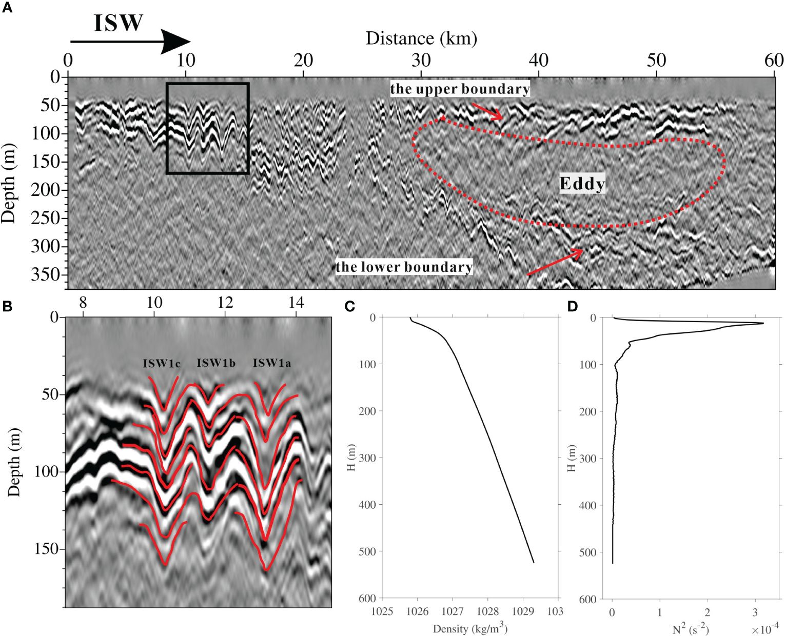
Figure 2 (A, B) The stacked section of L33 and the partial seismic section for ISW1s, respectively. The solid red lines are the picking reflection events, and the red dotted line is an eddy with arrows marking upper and lower boundaries. (C) Density profile. (D) Brunt–Vaisala frequency profile.
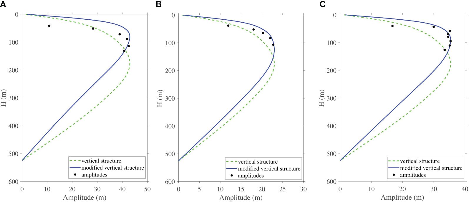
Figure 3 The vertical structures of (A) ISW1a, (B) ISW1b, and (C) ISW1c. The black dots represent the observed amplitudes, the green dotted lines represent the theoretical linear vertical structures, and the solid blue lines represent the theoretical nonlinear vertical structures with a first-order correction term (the corrected vertical structures). The water depth (the depth at which ISWs extend in the seawater) is 525 m.
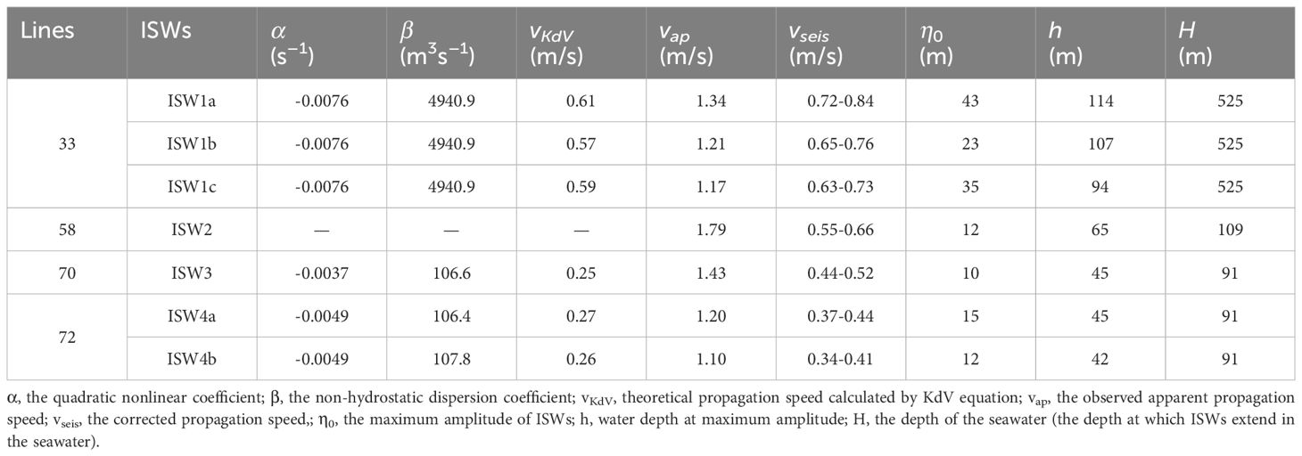
Table 1 The statistics of some characteristic parameters of ISWs.
The vertical structures of ISW3, ISW4a, and ISW4b fit well with the linear vertical structures. Their amplitudes decrease with increasing water depth within the depth range that seismic sections can reach. Figure 4 shows the seismic section and vertical structure of ISW3 on the continental shelf slope of L70. In the seismic section, ISW3 moves to the left along the shelf (Section 3.2.1). The waveform of ISW3 is symmetric. Its maximum amplitude is about 10 m at about 45 m of water depth. It is followed by a series of IWs with small amplitudes or oscillations, which usually means energy dissipation, decreasing the amplitude and speed of ISWs (Orr and Mignerey, 2003; Tang et al., 2018). ISW4a and ISW4b are only about 9 km apart from L72. They both move from left to right (toward the coast) along the direction of the shelf, but their waveform features are inconsistent (Figure 5A). We use corresponding hydrographic data (Figures 5B, C, E, F) to obtain the theoretical vertical amplitudes (Figures 5D, G). The waveform of ISW4b is symmetrical, and its vertical structure (Figure 5G) shows that the maximum amplitude is about 12 m at about 42 m water depth. Near the seafloor (91 m), the seismic event is parallel to the seafloor, and the amplitude is close to zero. It is worth noting that the amplitude of ISW4b increases abnormally near the water depth of 80 m, deviating from the linear vertical structure. ISW4a has an asymmetric waveform, and its front is less steep than its rear, which is directly related to the shoaling effects of ISWs. This process often causes the leading edge of standard depression ISWs to slow, the back edge to steepen, and gradually convert to elevation ISWs (Orr and Mignerey, 2003; Reeder et al., 2011). The calculated amplitude from the seismic section decreases gradually with increasing water depth. At about 45 m, the maximum amplitude is 15 m (Figure 5D). Due to the lack of shallow-water data, the maximum amplitude here is not necessarily the true value. Instead, it is the maximum amplitude that can be captured by the seismic data.
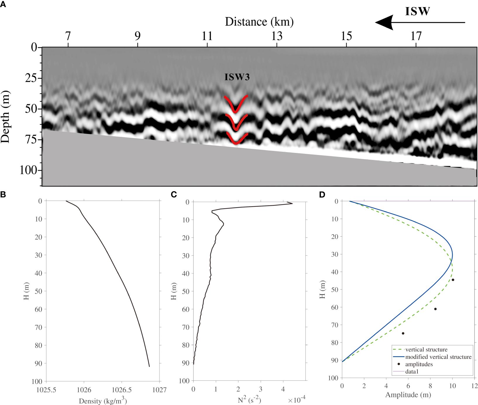
Figure 4 (A) Stacked section for L70. The solid red lines represent the picking reflection events. (B) Density profile. (C) Brunt–Vaisala frequency profile. (D) The vertical structure of ISW3. The black dots represent the observed amplitudes. The green dotted line represents the theoretical linear vertical structure. The solid blue line represents the theoretical nonlinear vertical structure with a first-order correction term. The depth of the seawater (the depth at which ISWs extend in the seawater) is 91 m.
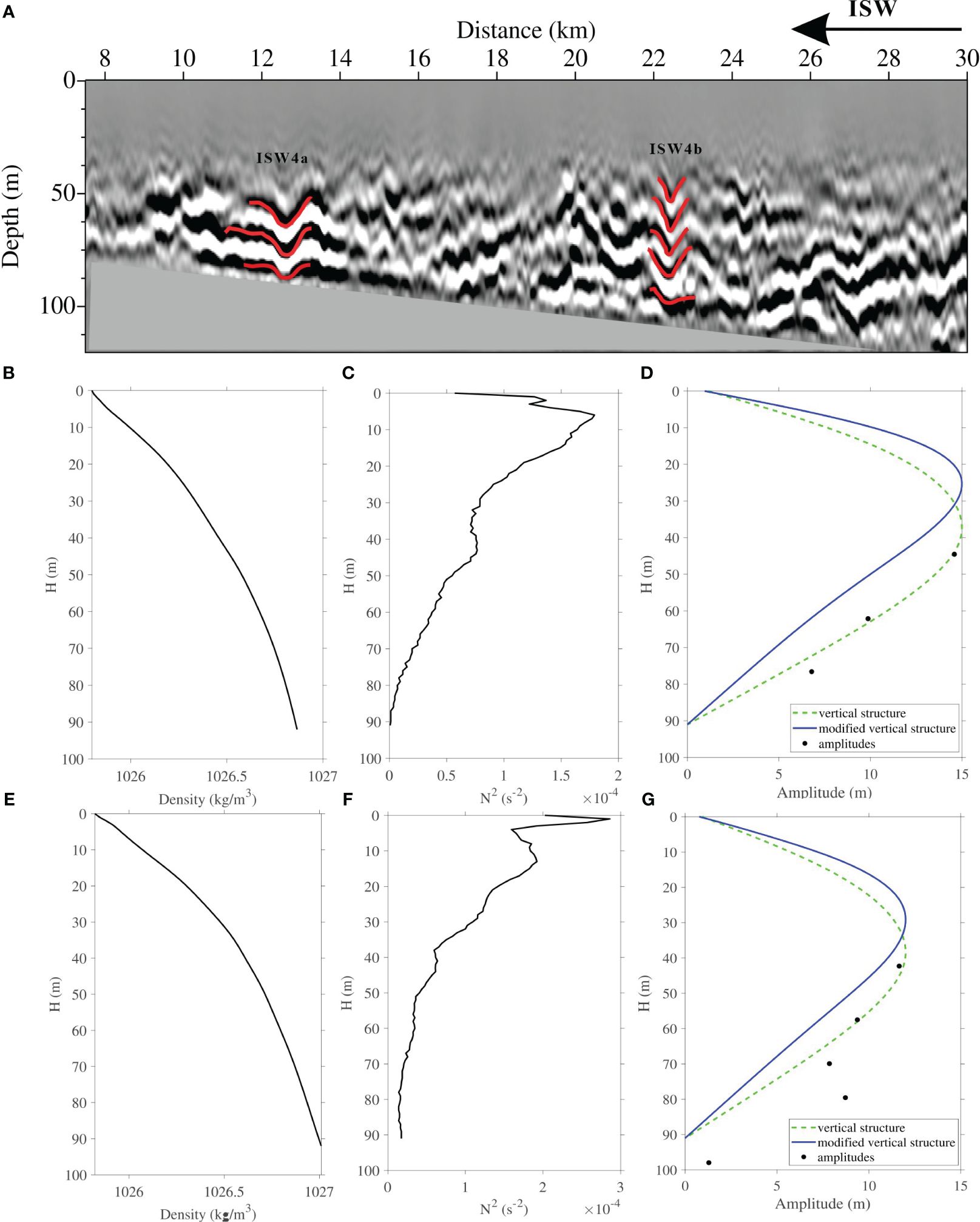
Figure 5 (A) Stacked section for L72. The solid red lines represent the picking reflection events. (B, C), (E, F) are the density and Brunt–Vaisala frequency profiles near ISW4a and ISW4b, respectively. In the vertical structures of (D) ISW4a and (G) ISW4b, the black dots represent the observed amplitudes; the green dotted line represents the theoretical linear vertical structure; the solid blue line represents the theoretical nonlinear vertical structure with a first-order correction term. The water depth (the depth at which ISWs extend in the water) is 91 m.
As Figure 6 shows, ISW2 on L58 does not conform to the linear vertical structure or the optimized nonlinear vertical structure. According to the seismic section, ISW2 is in flat terrain and has a shallow water depth of about 109 m (Figure 6A). The waveform is symmetrical, with the amplitude first increasing and then decreasing with water depth. However, near the seafloor, its amplitude is still about 11 m and has strong nonlinearity, which does not meet the condition of the rigid bottom (Equation 4). Higher-order equations are needed to better describe the dynamic process (Segur and Hammack, 1982; Kao et al., 1985).
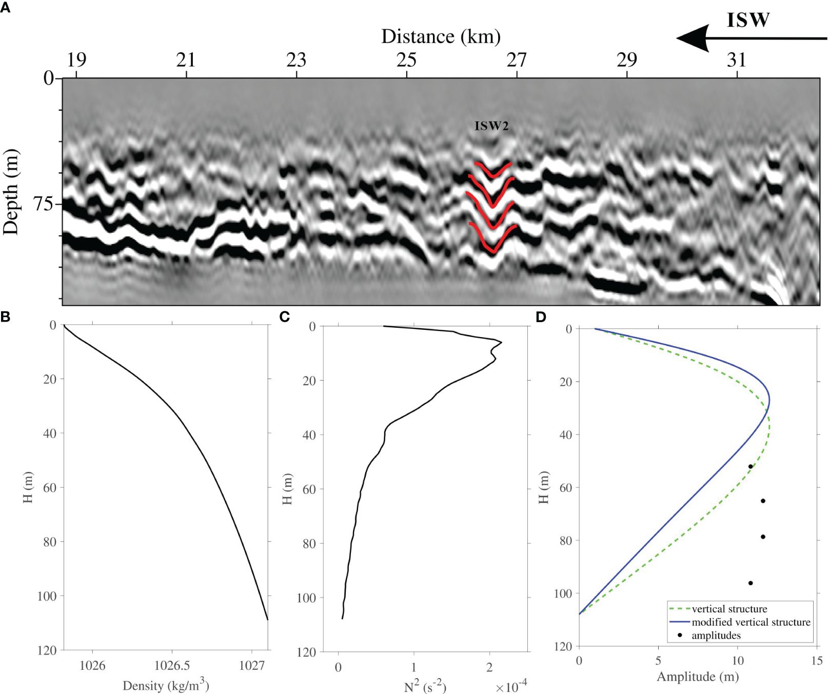
Figure 6 (A) Stacked section for L58. The solid red lines represent the picking reflection events. (B) Density profile. (C) Brunt–Vaisala frequency profile. (D) The vertical structure of ISW2. The black dots represent the observed amplitudes. The green dotted line represents the theoretical linear vertical structure. The solid blue line represents the theoretical nonlinear vertical structure with a first-order correction term. The depth of the seawater (the depth at which ISWs extend in the seawater) is 109 m.
The main difference between the two theoretical vertical structures is whether there is a first-order nonlinear correction term, which means that the nonlinearity of the vertical amplitude distribution is the main factor that determines which theory it fits (Section 2.3). According to the above analysis, ISW1s follow the nonlinear vertical structure with a first-order correction term, and their maximum amplitudes are much larger than other ISWs. ISW3 and ISW4s follow the linear vertical structure with relatively small amplitudes, while ISW2 follows the theoretical equation of higher order due to its strong nonlinearity. Thus, we suggest that, of these ISWs, ISW2 has the highest nonlinearity, followed by ISW1 and ISW3, and then ISW4a and ISW4b. The nonlinear coefficients of these ISWs can be estimated from Equation (2) (Table 1). ISW1s have the largest nonlinear coefficient of -0.0076 s–1, while ISW3, ISW4a, and ISW4b have relatively smaller nonlinear coefficients. As a result, the order of nonlinear strength is as follows: > > > > . Although ISW2, ISW3, and ISW4s have similar water depth, their nonlinearities are completely different. This indicates that, apart from water depth, the nonlinearity is influenced by local buoyancy frequency, and the strength of ocean stratification directly affects the vertical structure function ϕ. We can conclude that the key to keeping the shape of ISWs is the dynamic equilibrium between nonlinearity and dispersion. The strength of nonlinearity plays a dominant role in vertical structure. Also, the amplitude is usually linked to the strength of nonlinearity in a positive way.
In this study, we pick up shot-receiver pairs that capture the trough of ISWs on a series of migration Common Offset Gathers (COGs) with different offsets. This method was first proposed by Tang et al. (2014) to track ISWs with COGs. The slope k, corresponding to the shot-receiver pair curve, is then obtained by linear fitting (Figure 7). Finally, the relation is used to calculate the apparent phase speed vap, where dcmp is the CMP interval and dt is the shot time interval. Figure 7 shows the fitting curves of the 7 ISWs (ISW1a, ISW1b, ISW1c, ISW2, ISW3, ISW4a, and ISW4b) on the survey lines, respectively. Table 1 shows the resulting apparent phase velocities. One can see that the apparent velocities of ISW1s on L33 are arranged according to their magnitude, i.e., > > , and these waves travel in the same direction as the ship. The apparent phase speed of ISW1a is about 1.34 m/s. The apparent phase speed of ISW2 can reach 1.79 m/s. ISW3, ISW4a, and ISW4b are about 1.43, 1.20, and 1.10 m/s, respectively. They (ISW2 to ISW4s) all travel in the opposite direction to the ship. For how to determine the relationship between the direction of ISW and the ship, an interested reader is referred to Tang et al. (2014) and Fan et al. (2020) for more details.
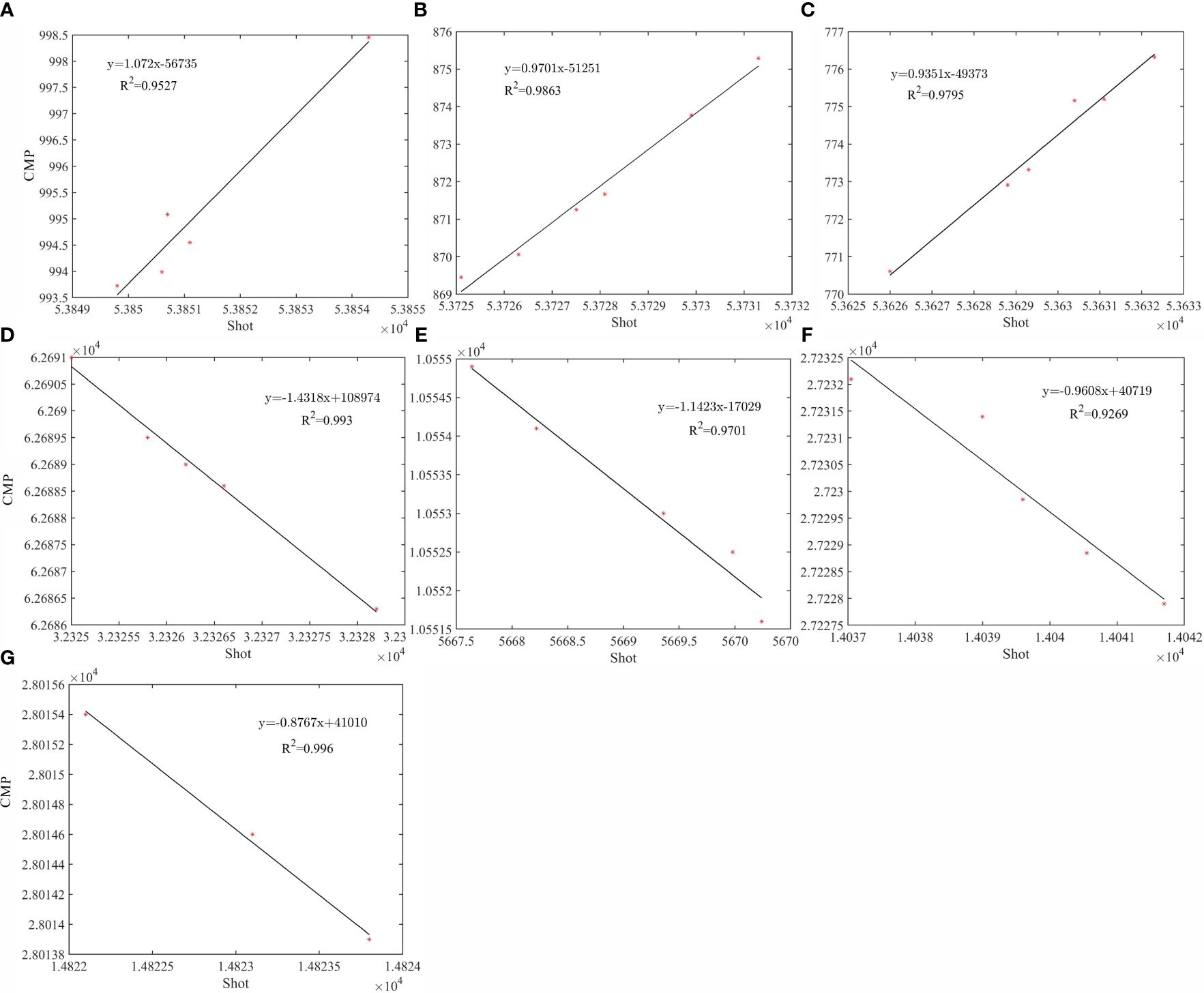
Figure 7 Fitting shot-receiver pairs. (A–G) Correspond to the fitting results of shot-receiver pairs for ISW1a, ISW1b, ISW1c, ISW2, ISW3, ISW4a, and ISW4b, respectively. The red asterisks are the picked shot-receiver pairs. The solid black lines are the fitting curves. R2 is the correlation coefficient (0-1), which describes the anastomoses between the data and the fitting curve. The larger the R2, the higher the degree of anastomoses.
By solving the internal wave vertical mode equation and the KdV equation, the theoretical linear phase speed c, the quadratic nonlinear coefficient α, and the dispersion coefficient β can be obtained. Then, the theoretical propagation speed vkdv is obtained according to equation . Table 1 shows our calculation results. We find that ISW1s have theoretical propagation speeds ranging from 0.57 to 0.61 m/s. The theoretical speed of ISW3 is 0.25 m/s. ISW4a and ISW4b have similar theoretical speeds of 0.26-0.27 m/s, with ISW4a being a little larger than ISW4b. Although ISW2 is unsuitable for low-order KdV equations, and cannot calculate theoretical phase speed, it is generally larger due to its strong nonlinearity.
There is a difference between the observed apparent speed vap and the theoretical phase speed vKdV. Because the propagation direction of the apparent speed vap is parallel to the direction of the seismic survey line, which does not necessarily represent the real propagation direction of ISWs. There is a certain angle between them; therefore, the apparent phase speed vap needs correction.
We use satellite SAR images to determine the actual propagation direction of the ISWs. The date of the seismic acquisition is 2000. We did not find satellite SAR images at that time. Thus, we used satellite SAR images acquired from January 2010 to October 2022 to map the distribution of IWs and ISWs and determine their propagation directions in the study area. Figure 8 shows two satellite SAR images offshore the South Island of New Zealand. We found the waves here had multiple sources, and the propagation directions were mainly about 22°-26° and 354°-360° (clockwise from due north). Combining the directions of the seismic lines shown in Figure 1, we can determine the actual propagation speed vseis following
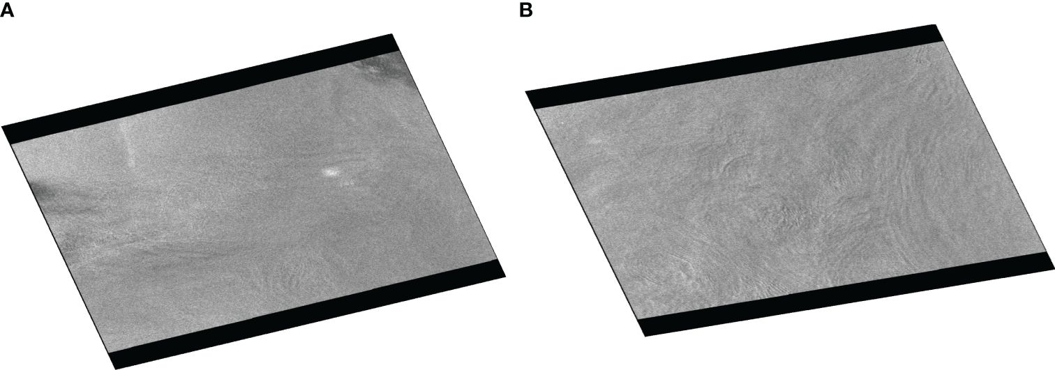
Figure 8 Satellite SAR images within the black rectangle in Figure 1A offshore the South Island of New Zealand from January 2010 to October 2022.
where θ is the angle between the seismic line and the propagation direction of ISWs. Based on the correction results, we found that, although the waves mostly travel across the isobaths toward the coast, their directions are slightly different. The propagation directions of ISW1s are mainly about 354°–360°. ISW2 (ISW3, and ISW4s) are mainly along about 22°–26°. Finally, the corrected propagation speed vseis of ISW1s (Equation 6), which ranges from 0.63 to 0.72 m/s, is close to the theoretical phase speed vKdV. The vseis of ISW3 and ISW4s also match the theoretical speeds.
Figure 9A shows the lateral changes in the amplitude of the ISW1s. The circles with different colors show the amplitude at different water depth ranges. The amplitude of ISW1c is mainly distributed in the horizontal range of 9.5-10 km, and the horizontal range of 11-11.5 km is the amplitude of ISW1b. The amplitude of ISW1a mainly concentrates in the horizontal range of 12-12.5 km. According to Figure 9A, the amplitudes of ISW1s in the same water depth range are in the order of ISW1a> ISW1c> ISW1b. That is, ISW1a has the largest amplitude, followed by ISW1c, and ISW1b has the smallest amplitude. This phenomenon is more obvious with the increase in water depth. But in shallow water, the amplitudes of the three ISWs within the same depth range are similar, and ISW1a is even smaller than the other two solitons. For example, the amplitude of ISW1a is slightly smaller than that of ISW1b when the water depth is 38-41 m.
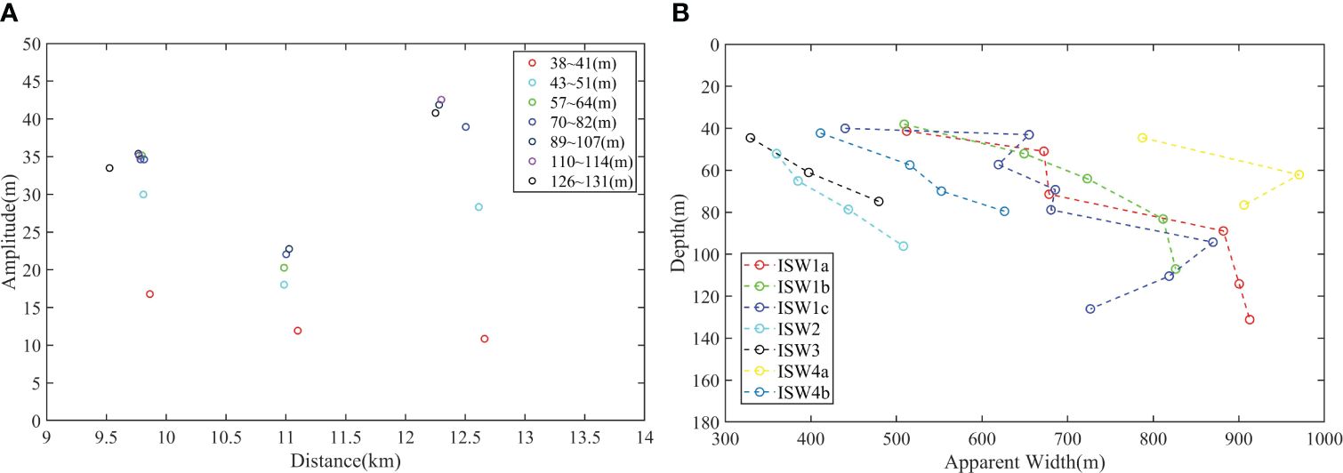
Figure 9 (A) Lateral variation of the amplitudes of ISW1s. Colored circles represent the amplitudes of ISW1s in different depth ranges. (B) Variation of apparent half-height width with depth. Colored marks represent the apparent half-height width of different ISWs. Part of the ISW4b waveform is not calculated due to severe asymmetry.
In addition to the lateral changes of the amplitudes, the apparent characteristic half-height widths of ISWs (the width of the trough at half amplitude) were obtained from the seismic sections. It is worth noting that the lateral information obtained from the seismic sections needs to be corrected. On the one hand, the ship and ISWs have different traveling speeds, which cause the Doppler effect to stretch or shorten the widths. On the other hand, there is an angle between them as mentioned above (Section 3.2). To eliminate the influence, we refer to the equation 1 mentioned by Bai et al. (2015), that is, , where vship is the speed of the ship. Table 2 lists their characteristic width Δ, apparent half-height width Lap, theoretical half-height width Lkdv, corrected half-height width L and Δ/L of at the maximum amplitude of ISWs. After width correction (Bai et al., 2015; Feng et al., 2021), the theoretical characteristic half-height width Lkdv matches L well, which proves that the correction is reasonable. Except for amplitude (Section 3.1), the characteristic half-height widths of ISW1s are also significantly larger than other ISWs, which also reflects the fact that the amplitude and width of ISW1s are positively correlated to some extent in order to maintain waveform stability, maintaining the dynamic equilibrium of the nonlinear effect and dispersion effect. Since this paper only studies the variation law of width with depth, Figure 9B uses the apparent half-height width Lap without width correction. We find that, in general, with increasing water depth, the ISWs waveform gradually widens. This is especially obvious for ISW4s that are close to the seafloor and can’t keep a stable waveform anymore, so their width increases sharply. It can reach a maximum of more than 900 m, and the event becomes roughly parallel to the seabed (Figure 5A).
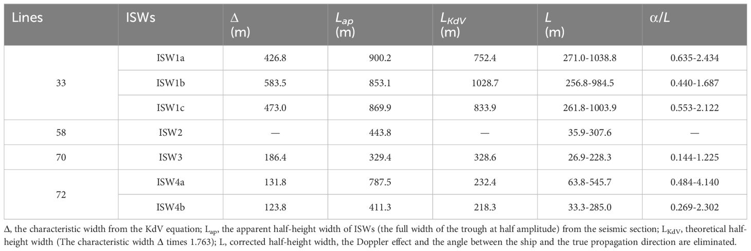
Table 2 Transverse structure characteristics of ISWs.
Combined with the theoretical model and the observation results (Section 3.2), it is considered that the relatively shallow water is more affected by the nonlinearity, which makes the phase speed of ISW2 much larger. However, ISW3 and ISW4s are close to the seafloor and may be affected by the topographic friction, so the corrected propagation speed is relatively small. ISW1s are in relatively deep water (about 525 m); thus, they are mainly affected by stratification and background current. It is barely affected by topography, so the propagation speed is relatively high. Moreover, the strong background currents (e.g., the Southland Current) may have an impact on the ISWs, which needs further dedicated research.
There is an eddy to the right of ISW1s (Figure 2A). The red dotted line region shows the eddy core. The arrows show the upper and lower boundaries of the eddy. They are at 50-90 m and 200-300 m, respectively. The width of the eddy is about 35 km, and its thickness is about 225 m. The eddy tilts to the right, and the reflection layers at the boundaries are developed well. The upper boundary extends horizontally, while the lower boundary is more tilted and has strong fluctuations. The strong fluctuations indicate that IWs are developing here. The seismic reflections of the eddy core are usually weak and chaotic, indicating that the water in the core is well mixed, and the temperature and salinity are homogeneous. Combining with Figure 10, we found that the temperature and salinity present a slanted ellipsoid shape at a depth of 50-250 m on the right side of the section (172.2°E-172.4°E), which is a typical eddy indicator. The temperature (salinity) at the core is about 12°C (34.48 psu). The temperature changes near the upper and lower boundaries are about 0.5-1°C, the salinity changes are 0.2-0.4 psu, and the thermocline deepens to about 125 m. Based on the horizontal distribution diagram of geostrophic speed and sea surface height (SSH) (Figure 11), there are two cyclonic eddies in the northeast direction of ISW1s (red pentagram), which also indicates that eddies in this area are developed.
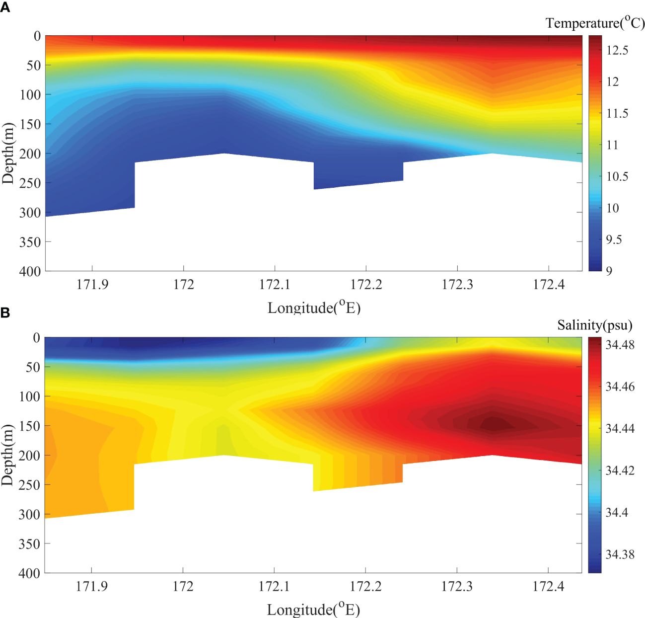
Figure 10 (A) Temperature and (B) Salinity along L33.
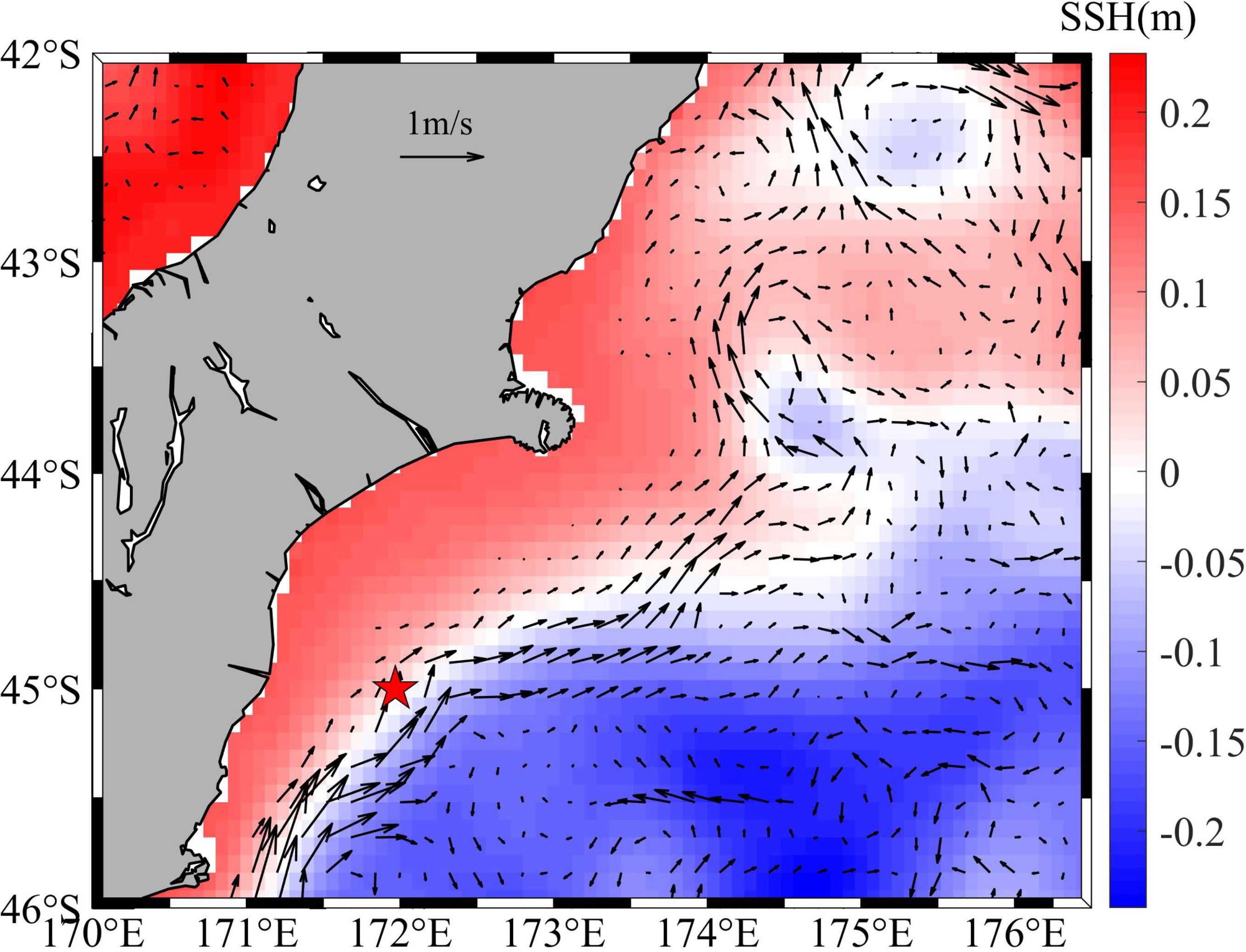
Figure 11 Background colors show sea surface height (SSH), and arrows represent the geostrophic currents at 100 m. The red pentagram represents ISW1s.
As shown in Figure 12A, there is also a right-tilted eddy on the right side of the seismic section of L23. The eddy’s size and shape are identical to those found on L33. Both its upper and lower boundaries have strong reflections. Because the two survey lines are close to each other and the acquisition time is only about 15 days apart, it is presumed to be the same eddy. Compared with the side boundary, the reflection layers of the upper and lower boundaries are stronger and accompanied by strong fluctuations, indicating that IWs (or ISWs) are widely developed. Among them, ISWs (packets) with small amplitudes are developed on the upper boundary of the eddy (Figure 12B), and part of the vertical structures weaken or even disappear when they cross the boundary into the eddy, which is consistent with the observation results (Xu et al., 2020). IWs at the lower boundary are manifested as a series of high-frequency, small-amplitude oscillations, and the overall distribution of the reflection events tilts under the influence of the eddy (Figure 12C). Therefore, compared with other positions of the eddy, the horizontal wavenumber spectrum may be slightly higher than the GM spectrum, with enhanced internal wave energy (Holbrook and Fer, 2005).
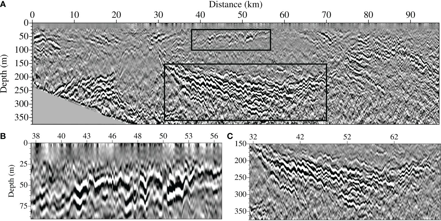
Figure 12 (A) Stacked section for L23. (B, C) Partially enlarged views in the boxes.
IWs and ISWs that pass through the eddy or develop at the boundary of the eddy will more or less affect the eddy. For example, ISWs in this example even affect the inside of the eddy, which may bring seawater into the eddy. Suppose ISWs pass through the eddy. In that case, it also brings a small amount of eddy core water. The exchange of the core water and the surrounding seawater may speed ocean mixing.
In this paper, the original multi-channel seismic data offshore the South Island of New Zealand was reprocessed. On four seismic survey lines, four first baroclinic mode depression ISWs (packets) were found. The amplitudes were extracted from the seismic sections and compared with the two theoretical vertical structures. We found that ISW1s fit the first-order nonlinear vertical structure, ISW3s and ISW4s fit the linear vertical structure well, but ISW2 doesn’t fit either structure. The main difference between these two theoretical vertical structures is whether or not there is a first-order nonlinear correction term. This means that the nonlinearity of the vertical amplitude distribution is the main factor. The nonlinear strength is ranked as follows: > > > > . Due to the strong nonlinearity that does not apply to the low-order KdV equation, ISW2 needs the higher-order equation. ISW1s is more nonlinear than ISW3 and ISW4s, so it fits the nonlinear vertical structure. The amplitude is generally proportional to the nonlinear strength without considering the water depth, background flow, and other conditions. Therefore, the vertical amplitude of ISW1s is much larger than that of other ISWs. We used two different methods to calculate the propagation speed of ISWs. The theoretical propagation speed of ISW1s is 0.57–0.61 m/s, among which ISW1a is the largest. The theoretical propagation speed of ISW3 is about 0.25 m/s, and the theoretical propagation speed of ISW4s is 0.26 to 0.27 m/s. Based on satellite remote sensing images, it is inferred that the propagation direction of ISW1s (about 354°-360°) may be different from other ISWs (about 22°-26°), though they both travel across the isobaths towards the coast. The corrected propagation speed vseis matches the theoretical speed vKdV.
We further investigate the lateral structural changes of ISWs. The amplitude of ISW1a is the largest, followed by ISW1c, and the amplitude of ISW1b is the smallest in the same water depth. This phenomenon becomes more obvious with the increase in water depth. In addition, we found that the half-height width of ISW1s was much larger than other ISWs, and the waveform of ISWs gradually widened with increasing water depth.
The eddy may interact with IWs and ISWs. In this example, the small-amplitude ISWs (packets) are developed on the upper boundary of the eddy, and their vertical amplitudes weaken or even disappear when they cross the boundary into the eddy. IWs at the lower boundary of the eddy are a series of high-frequency oscillations. The overall distribution of the reflection events tilted under the influence of the eddy, which is expected to enhance internal wave energy. IWs and ISWs developed at the edge of the eddy can affect the eddy’s boundary and inside, which may promote the mixing of the core water and the external water, thus changing the thermohaline properties of seawater. Therefore, IWs and ISWs also have a certain degree of influence on the eddy.
The original contributions presented in the study are included in the article/supplementary material. Further inquiries can be directed to the corresponding author.
LM: Conceptualization, Investigation, Methodology, Writing – original draft, Writing – review & editing. KZ: Conceptualization, Methodology, Writing – review & editing. HS: Conceptualization, Funding acquisition, Writing – review & editing. ML: Data curation, Investigation, Validation, Writing – review & editing.
The author(s) declare financial support was received for the research, authorship, and/or publication of this article. This study was supported by the National Natural Science Foundation of China (Grant 42176061, and 41976048).
The authors thank Prof. Zhongxiang Zhao (University of Washington) for his constructive suggestions that greatly improved this study. We are grateful to handling editor Mr. Leonardo Azevedo and two reviewers for their constructive reviews and comments on the manuscript. Thanks to the Marine Geoscience Data System (Marine Geoscience Data System) for providing reflection seismic data (http://www.marine-geo.org/). Thanks to the National Oceanic and Atmospheric Administration (https://www.ncei.noaa.gov/products/world-ocean-database) for providing historical CTD data, and thanks to the U.S. Naval Research Laboratory for providing HYCOM thermohaline reanalysis products (https://www.hycom.org/hycom), and the Marine Environment Monitoring Service Center (Copernicus Marine Environment Monitoring The Service, the thermohaline CMEMS) for presenting analysis data (http://marine.copernicus.eu/services-portfolio/access-to-products/). The SAR data is available for download at the Alaska Satellite News Agency (ASF) (https://search.asf.alaska.edu/#/). The ASF’s support for this study is greatly appreciated.
The authors declare that the research was conducted in the absence of any commercial or financial relationships that could be construed as a potential conflict of interest.
All claims expressed in this article are solely those of the authors and do not necessarily represent those of their affiliated organizations, or those of the publisher, the editors and the reviewers. Any product that may be evaluated in this article, or claim that may be made by its manufacturer, is not guaranteed or endorsed by the publisher.
Apel J. R., Holbrook J. R., Liu A. K., Tsai J. J. (1985). The Sulu Sea internal soliton experiment. J. Phys. Oceanogr. 15, 1625–1651. doi: 10.1175/1520-0485(1985)015<1625:Tssise>2.0.Co;2
Bai X., Liu Z., Zheng Q., Hu J., Lamb K. G., Cai S. (2019). Fission of shoaling internal waves on the northeastern shelf of the south China sea. J. Geophys. Res.-Oceans. 124, 4529–4545. doi: 10.1029/2018jc014437
Bai Y., Song H., Guan Y., Yang S. (2017). Estimating depth of polarity conversion of shoaling internal solitary waves in the northeastern South China Sea. Cont. Shelf Res. 143, 9–17. doi: 10.1016/j.csr.2017.05.014
Bai Y., Song H., Guan Y., Yang S., Liu B., Chen J., et al. (2015). Nonlinear internal solitary waves in the northeast South China Sea near Dongsha Atoll using seismic oceanography. Chin. Sci. Bull. 60, 944–951. doi: 10.1360/N972014-00911
Boegman L., Stastna M. (2019). Sediment resuspension and transport by internal solitary waves. Annu. Rev. Fluid Mech. 51, 129–154. doi: 10.1146/annurev-fluid-122316-045049
Buffett G. G., Krahmann G., Klaeschen D., Schroeder K., Sallarès V., Papenberg C., et al. (2017). Seismic oceanography in the Tyrrhenian Sea: Thermohaline staircases, eddies, and internal waves. J. Geophys. Res.-Oceans. 122, 8503–8523. doi: 10.1002/2017jc012726
Cai S., Xu J., Liu J., Chen Z., Xie J., Li J., et al. (2015). Retrieval of the maximum horizontal current speed induced by ocean internal solitary waves from low resolution time series mooring data based on the KdV theory. Ocean Eng. 94, 88–93. doi: 10.1016/j.oceaneng.2014.11.023
Chiswell S. M., Bostock H. C., Sutton P. J. H., Williams M. J. M. (2015). Physical oceanography of the deep seas around New Zealand: a review. N. Z. J. Mar. Freshw. Res. 49, 286–317. doi: 10.1080/00288330.2014.992918
Cooper J. K., Gorman A. R., Bowman M. H., Smith R. O. (2021). Temporal variability of thermohaline fine-structure associated with the subtropical front off the southeast coast of New Zealand in high-frequency short-streamer multi-channel seismic data. Front. Mar. Sci. 8. doi: 10.3389/fmars.2021.751385
Djordjevic V. D., Redekopp L. G. (1978). The fission and disintegration of internal solitary waves moving over two-dimensional topography. J. Phys. Oceanogr. 8, 1016–1024. doi: 10.1175/1520-0485(1978)008<1016:Tfadoi>2.0.Co;2
Duda T. F., Lynch J. F., Irish J. D., Beardsley R. C., Ramp S. R., Chiu C. S., et al. (2004). Internal tide and nonlinear internal wave behavior at the continental slope in the northern South China Sea. IEEE J. Ocean. Eng. 29, 1105–1130. doi: 10.1109/joe.2004.836998
Fan W., Song H., Gong Y., Sun S., Zhang K., Wu D., et al. (2021). The shoaling mode-2 internal solitary waves in the Pacific coast of Central America investigated by marine seismic survey data. Cont. Shelf Res. 212, 104318. doi: 10.1016/j.csr.2020.104318
Fan W., Song H., Zhang K., HSU H., Gong Y., Sun S. (2020). Seismic oceanography study of internal solitary waves in the northeastern South China Sea Basin. Chin. J. Geophys.-Chinese Ed. 63, 2644–2657. doi: 10.6038/cjg2020N0358
Farmer D., Armi L. (1999). The generation and trapping of solitary waves over topography. Science 283, 188–190. doi: 10.1126/science.283.5399.188
Feng Y., Tang Q., Li J., Sun J., Zhan W. (2021). Internal solitary waves observed on the continental shelf in the northern South China Sea from acoustic backscatter data. Front. Mar. Sci. 8. doi: 10.3389/fmars.2021.734075
Fliegel M., Hunkins K. (1975). Internal wave dispersion calculated using the Thomson-Haskell method. J. Phys. Oceanogr. 5, 541–548. doi: 10.1175/1520-0485(1975)005<0541:Iwdcut>2.0.Co;2
Geng M., Song H., Guan Y., Bai Y. (2019). Analyzing amplitudes of internal solitary waves in the northern South China Sea by use of seismic oceanography data. Deep-Sea Res. Part I-Oceanogr. Res. Pap. 146, 1–10. doi: 10.1016/j.dsr.2019.02.005
Geng M. H., Song H. B., Guan Y. X., Chen J. (2018). Research on the distribution and characteristics of the nepheloid layers in the northern South China Sea by use of seismic oceanography method. Chin. J. Geophys.-Chinese Ed. 61, 636–648. doi: 10.6038/cjg2018L0662
Gong Y., Song H., Zhao Z., Guan Y., Kuang Y. (2021a). On the vertical structure of internal solitary waves in the northeastern South China Sea. Deep-Sea Res. Part I-Oceanogr. Res. Pap. 173, 103550. doi: 10.1016/j.dsr.2021.103550
Gong Y., Song H., Zhao Z., Guan Y., Zhang K., Kuang Y., et al. (2021b). Enhanced diapycnal mixing with polarity-reversing internal solitary waves revealed by seismic reflection data. Nonlinear Process Geophys. 28, 445–465. doi: 10.5194/npg-28-445-2021
Gorman A. R., Smillie M. W., Cooper J. K., Bowman M. H., Vennell R., Holbrook W. S., et al. (2018). Seismic characterization of oceanic water masses, water mass boundaries, and mesoscale eddies SE of New Zealand. J. Geophys. Res.-Oceans. 123, 1519–1532. doi: 10.1002/2017jc013459
Holbrook W. S. (2003). Thermohaline fine structure in an oceanographic front from seismic reflection profiling. Science 301, 821–824. doi: 10.1126/science.1085116
Holbrook W. S., Fer I. (2005). Ocean internal wave spectra inferred from seismic reflection transects. Geophys. Res. Lett. 32, L15604. doi: 10.1029/2005gl023733
Jackson C. (2007). Internal wave detection using the Moderate Resolution Imaging Spectroradiometer (MODIS). J. Geophys. Res.-Oceans. 112, C11012. doi: 10.1029/2007JC004220
Kao T. W., Pan F.-S., Renouard D. (1985). Internal solitons on the pycnocline: generation, propagation, and shoaling and breaking over a slope. J. Fluid Mech. 159, 19–53. doi: 10.1017/S0022112085003081
Klymak J. M., Gregg M. C. (2004). Tidally generated turbulence over the Knight Inlet Sill. J. Phys. Oceanogr. 34, 1135–1151. doi: 10.1175/1520-0485(2004)034<1135:Tgtotk>2.0.Co;2
Kurkina O., Rouvinskaya E., Kurkin A., Giniyatullin A., Pelinovsky E. (2018). Vertical structure of the velocity field induced by mode-I and mode-II solitary waves in a stratified fluid. Eur. Phys. J. E. 41, 47. doi: 10.1140/epje/i2018-11654-3
Liao G., Hua Xu X., Liang C., Dong C., Zhou B., Ding T., et al. (2014). Analysis of kinematic parameters of internal solitary waves in the Northern South China Sea. Deep-Sea Res. Part I-Oceanogr. Res. Pap. 94, 159–172. doi: 10.1016/j.dsr.2014.10.002
Lien R.-C., D’Asaro E. A., Henyey F., Chang M.-H., Tang T.-Y., Yang Y.-J. (2012). Trapped core formation within a shoaling nonlinear internal wave. J. Phys. Oceanogr. 42, 511–525. doi: 10.1175/2011JPO4578.1
Liu A. K., Chang Y. S., Hsu M.-K., Liang N. K. (1998). Evolution of nonlinear internal waves in the east and south China Seas. J. Geophys. Res.-Oceans. 103, 7995–8008. doi: 10.1029/97JC01918
Maxworthy T. (1979). A note on the internal solitary waves produced by tidal flow over a three-dimensional ridge. J. Geophys. Res.-Oceans. 84, 338–346. doi: 10.1029/JC084iC01p00338
Munk W., Wunsch C. (1998). Abyssal recipes II: energetics of tidal and wind mixing. Deep-Sea Res. Part I-Oceanogr. Res. Pap. 45, 1977–2010. doi: 10.1016/S0967-0637(98)00070-3
Neil H. L., Carter L., Morris M. Y. (2004). Thermal isolation of Campbell Plateau, New Zealand, by the Antarctic Circumpolar Current over the past 130 kyr. Paleoceanography 19, PA4008. doi: 10.1029/2003PA000975
Orr M. H., Mignerey P. C. (2003). Nonlinear internal waves in the South China Sea: Observation of the conversion of depression internal waves to elevation internal waves. J. Geophys. Res.-Oceans. 108, 3064. doi: 10.1029/2001JC001163
Ostrovsky L. A., Stepanyants Y. A. (1989). Do internal solutions exist in the ocean? Rev. Geophys. 27, 293–310. doi: 10.1029/RG027i003p00293
Ramp S. R., Tswen Yung T., Duda T. F., Lynch J. F., Liu A. K., Ching-Sang C., et al. (2004). Internal solitons in the northeastern south China Sea. Part I: sources and deep water propagation. IEEE J. Ocean. Eng. 29, 1157–1181. doi: 10.1109/JOE.2004.840839
Reeder D. B., Ma B. B., Yang Y. J. (2011). Very large subaqueous sand dunes on the upper continental slope in the South China Sea generated by episodic, shoaling deep-water internal solitary waves. Mar. Geol. 279, 12–18. doi: 10.1016/j.margeo.2010.10.009
Ruddick B., Song H., Dong C., Pinheiro L. (2009). Water column seismic images as maps of temperature gradient. Oceanography 22, 192–205. doi: 10.5670/oceanog.2009.19
Segur H., Hammack J. L. (1982). Soliton models of long internal waves. J. Fluid Mech. 118, 285–304. doi: 10.1017/S0022112082001086
Song H., Chen J., Pinheiro L. M., Ruddick B., Fan W., Gong Y., et al. (2021a). Progress and prospects of seismic oceanography. Deep-Sea Res. Part I-Oceanogr. Res. Pap. 177, 103631. doi: 10.1016/j.dsr.2021.103631
Song H., Gong Y., Yang S., Guan Y. (2021b). Observations of internal structure changes in shoaling internal solitary waves based on seismic oceanography method. Front. Mar. Sci. 8. doi: 10.3389/fmars.2021.733959
Song H., Pinheiro L. M., Ruddick B., Teixeira F. C. (2011). Meddy, spiral arms, and mixing mechanisms viewed by seismic imaging in the Tagus Abyssal Plain (SW Iberia). J. Mar. Res. 69, 827–842. doi: 10.1357/002224011799849309
Tang Q., Hobbs R., Wang D., Sun L., Zheng C., Li J., et al. (2015). Marine seismic observation of internal solitary wave packets in the northeast South China Sea. J. Geophys. Res.-Oceans. 120, 8487–8503. doi: 10.1002/2015jc011362
Tang Q., Hobbs R., Zheng C., Biescas B., Caiado C. (2016). Markov Chain Monte Carlo inversion of temperature and salinity structure of an internal solitary wave packet from marine seismic data. J. Geophys. Res.-Oceans. 121, 3692–3709. doi: 10.1002/2016jc011810
Tang Q., Wang C., Wang D., Pawlowicz R. (2014). Seismic, satellite, and site observations of internal solitary waves in the NE South China Sea. Sci. Rep. 4, 5374. doi: 10.1038/srep05374
Tang Q., Xu M., Zheng C., Xu X., Xu J. (2018). A locally generated high-mode nonlinear internal wave detected on the shelf of the northern South China Sea from marine seismic observations. J. Geophys. Res.-Oceans. 123, 1142–1155. doi: 10.1002/2017jc013347
Wei J., Gunn K. L., Reece R. (2022). Mid-ocean ridge and storm enhanced mixing in the central south atlantic thermocline. Front. Mar. Sci. 8. doi: 10.3389/fmars.2021.771973
Wunsch C. (2004). Vertical mixing, energy, and the general circulation of the oceans. Annu. Rev. Fluid Mech. 36, 281–314. doi: 10.1146/annurev.fluid.36.050802.122121
Xu J., He Y., Chen Z., Zhan H., Wu Y., Xie J., et al. (2020). Observations of different effects of an anti-cyclonic eddy on internal solitary waves in the South China Sea. Prog. Oceanogr. 188, 102422. doi: 10.1016/j.pocean.2020.102422
Yang S., Song H., Coakley B., Zhang K., Fan W. (2022). A mesoscale eddy with submesoscale spiral bands observed from seismic reflection sections in the Northwind Basin, Arctic Ocean. J. Geophys. Res.-Oceans. 127, e2021JC017984. doi: 10.1029/2021jc017984
Keywords: internal solitary waves, KdV equation, waveform, propagation speed, eddies, seismic oceanography
Citation: Meng L, Zhang K, Song H and Liu M (2024) Seismic oceanography of internal solitary waves offshore the South Island, New Zealand. Front. Mar. Sci. 11:1376945. doi: 10.3389/fmars.2024.1376945
Received: 26 January 2024; Accepted: 24 June 2024;
Published: 09 July 2024.
Edited by:
Juan Jose Munoz-Perez, University of Cádiz, SpainReviewed by:
Zhuangcai Tian, China University of Mining and Technology, ChinaCopyright © 2024 Meng, Zhang, Song and Liu. This is an open-access article distributed under the terms of the Creative Commons Attribution License (CC BY). The use, distribution or reproduction in other forums is permitted, provided the original author(s) and the copyright owner(s) are credited and that the original publication in this journal is cited, in accordance with accepted academic practice. No use, distribution or reproduction is permitted which does not comply with these terms.
*Correspondence: Haibin Song, aGJzb25nQHRvbmdqaS5lZHUuY24=
Disclaimer: All claims expressed in this article are solely those of the authors and do not necessarily represent those of their affiliated organizations, or those of the publisher, the editors and the reviewers. Any product that may be evaluated in this article or claim that may be made by its manufacturer is not guaranteed or endorsed by the publisher.
Research integrity at Frontiers
Learn more about the work of our research integrity team to safeguard the quality of each article we publish.