A hybrid CEEMDAN-VMD-TimesNet model for significant wave height prediction in the South Sea of China

Accurate prediction of significant wave height is of great reference value for wave energy generation. However, due to the non-linearity and non-stationarity of significant wave height, traditional algorithms face difficulties in achieving satisfactory prediction results. In this study, a hybrid CEEMDAN-VMD-TimesNet model is proposed for non-stationary significant wave height prediction. Based on the significant wave height in the South Sea of China, the performance of the SVM model, the GRU model, the LSTM model, the TimesNet model, the CEEMDAN-TimesNet model and the CEEMDAN-VMD-TimesNet model are compared in terms of multi-step prediction. It is found that the prediction accuracy of the TimesNet model is higher than that of the SVM model, the GRU model and the LSTM model. The non-stationarity of significant wave height is reduced by CEEMDAN decomposition. Thus, the CEEMDAN-TimesNet model performs better than the TimesNet model in predicting significant wave height. The prediction accuracy of the CEEMDAN-VMD-TimesNet model is further improved by employing VMD for the secondary decomposition of components with high and moderate complexity. Additionally, the CEEMDAN-VMD-TimesNet model can accurately predict trends and extreme values of significant wave height with minimal phase shifts even during typhoon periods. The results demonstrate that the CEEMDAN-VMD-TimesNet model exhibits superiority in predicting significant wave height.

1 Introduction

More than 70% of the world is composed of oceans. Wave energy, as a clean and renewable energy source (Reikard et al., 2015), is crucial for addressing the energy crisis. For wave energy generation, the significant wave height is a crucial metric (Ali and Prasad, 2019). As a result, there has always been a great deal of focus on accurately predicting significant wave height (Deo et al., 2001). However, predicting significant wave height is challenging. In particular, during extreme weather conditions such as typhoons, the significant wave height undergoes rapid changes, posing a significant challenge to accurate prediction.

So far, experts and researchers from various countries have attempted to establish numerical models to simulate significant wave height (Reikard et al., 2017). Reikard and Rogers (2011) tried to predict significant wave height in the Pacific region and the Gulf of Mexico using the SWAN model. It was found that when the forecast time exceeds 6 hours, the SWAN model’s prediction accuracy surpasses that of mathematical models. Chen et al. (2018) created a wave-current system that combined FVCOM with SWAN. This system allowed for on-line, two-way coupling and was also more computationally efficient and user-friendly for simulating wave-current interactions near the coast. Amunugama et al. (2020) employed the COAWST model to simulate multiple intense typhoons in Japan and found that the COAWST model effectively reproduced typhoon phenomena, storm surges, and wave height. Vijayan et al. (2023) utilized the dynamic coupling of SWAN and ADCIRC to simulate Hurricane Michael. They observed that the accuracy of the simulation was significantly improved by the dynamic coupling model of SWAN and ADCIRC.

However, traditional physics models often require high accuracy in terrain and boundary conditions and also require a significant amount of computing time (Wang et al., 2018). Consequently, as computer technology advances, an increasing number of researchers have shown a strong interest in machine learning. Soares and Cunha (2000) utilized a bivariate AR model incorporating significant wave height and average wave period to predict significant wave height at two adjacent stations in Portugal. Agrawal and Deo (2002) employed ARMA and ARIMA models to predict significant wave height at a nearshore location in India at intervals of 3, 6, 12, and 24 hours. By using Support Vector Machine (SVM), Mahjoobi and Mosabbeb (2009) successfully predicted significant wave height in Lake Michigan with acceptable accuracy.

Neural networks, known for the superiority in handling non-linear problems, have gained popularity among researchers. A growing number of experts have adopted the usage of neural networks for the purpose of predicting significant wave height. Chang et al. (2011) developed an Artificial Neural Network (ANN) model for typhoon waves, using local wind and simulated waves as the two critical factors for the proposed ANN model’s input parameters. With the development of deep learning, long short-term memory (LSTM) network (Hochreiter and Schmidhuber, 1997) has gained attention. LSTM network can effectively capture the long-term dependencies in time series sequences and utilize historical data for prediction. Fan et al. (2020) used the wind speed data from the last 4 hours, together with the wave height and wind direction data from the previous 1 hour, as input variables to predict significant wave height at 10 distinct stations with varying oceanic environmental circumstances. The findings demonstrated that the LSTM model was capable of attaining precise prediction outcomes. Bethel et al. (2022) utilized LSTM to predict significant wave height during hurricanes Dorian, Sandy, and Igor. They found that the LSTM model is highly suitable for swiftly forecasting hurricane-forced wave height, with significantly lower computational expenses when compared to numerical wave models. Song et al. (2022) developed a high spatial and temporal resolution regional significant wave height prediction model based on the ConvLSTM model. Additionally, the Mask method and Replace mechanism were applied to improve the model’s long-term forecasting capabilities. Gate recurrent unit (GRU), as a variant of LSTM, has also been put into use. Meng et al. (2021) proposed a BiGRU network for wave height prediction during TC. The prediction by BiGRU of 10 buoys during a new typhoon was compared with machine learning models. The findings indicated that the BiGRU’s predictive ability is stable, particularly for predicting 24 hours in advance. Li et al. (2022) predicted significant wave height at six stations along the coast of China. The experimental results showed that for a 3-hour forecast, the GRU network exhibited stronger robustness compared to the LSTM network. The prediction accuracy of significant wave height has been improved by the application of these deep learning techniques.

Unlike traditional convolutional neural networks and recurrent neural networks, the transformer utilized the attention mechanism to capture data features and has achieved good results (Vaswani et al., 2017). Shortly after, the Informer was proposed, which greatly reduced the computation time through the ProbSparse self-attention mechanism and the self-attention distilling (Zhou et al., 2021). Based on the Auto-Correlation mechanism, the Autoformer was successfully proposed. The accurate prediction was achieved using the Autoformer (Wu et al., 2021). Recently, the one-dimensional time series was transformed into a two-dimensional tensor to capture intra-period and inter-period changes. Following this approach, the TimesNet model was constructed, which achieved significant progress in time series prediction (Wu et al., 2022).

Due to the non-stationarity of significant wave height data, simply altering the network structure often fails to solve the problem effectively. Therefore, scholars have considered decomposing the significant wave height data to reduce the non-stationarity. Empirical mode decomposition (EMD) has demonstrated excellent performance in handling non-linear and non-stationary data (Huang et al., 1998). Duan et al. (2016) utilized EMD-AR to predict significant wave height. The results proved the effectiveness of EMD in handling non-linear and non-stationary significant wave height. Hao et al. (2022) decomposed significant wave height using EMD and then used the LSTM to predict the decomposed components. They found that the EMD-LSTM model significantly improves prediction accuracy. Compared to EMD, ensemble empirical mode decomposition (EEMD) exhibits greater robustness in terms of sampling and noise (Wu and Huang, 2009). EEMD and LSTM were used to propose a real-time TC wave height forecasting system (ATDNNS). The experimental findings revealed that ATDNNS performed much better compared to the baseline model and had the potential to address the issue of poor initial forecast performance in numerical models (Meng et al., 2022). The significant wave height in the Indian Ocean region was predicted using EEMD-LSTM. It was found that the prediction results by EEMD-LSTM were more accurate compared to the prediction results by EMD-LSTM (Song et al., 2023). Variational mode decomposition (VMD) is another improved version of EMD, demonstrating enhanced signal processing capabilities (Dragomiretskiy and Zosso, 2013). Yang and Huang (2022) introduced an approach using VMD to estimate the significant wave height from X-band marine radar images. They found that VMD-based linear fitting technique outperformed the conventional EEMD-based linear fitting technique in terms of accuracy. Sharma et al. (2023) incorporated a hybrid VMD-BiLSTM into the ship’s autopilot system. The experimental results showed that deep learning models were able to more correctly capture the observable variational components in the data due to VMD-based data decomposition. Zhao et al. (2023) established a VMD-LSTM/GRU hybrid model to predict significant wave height in the east coast of China accurately. The finding demonstrated that VMD can handle non-linear and non-stationary significant wave height effectively.

Although previous prediction models based on single decomposition such as VMD have achieved notable outcomes, there is potential for further improvement. This article proposes a CEEMDAN-VMD-TimesNet model that combines the two-layer decomposition framework with the TimesNet model. We first decompose the original significant wave height into IMFs and a residual component by using complete ensemble empirical mode decomposition with adaptive noise (CEEMDAN). Next, we reconstruct each IMF and residual with sample entropy algorithm and K-means clustering algorithm. The VMD is used to decompose the high and medium complexity components that cause the main errors. Compared to the single decomposition, the secondary decomposition can better reduce the non-stationarity of significant wave height. In addition, we adopt TimesNet model as the main model for wave height prediction. This is due to the fact that the TimesNet model can capture the short-term temporal patterns within a period and the long-term trends of different periods well, which is conducive to improving the prediction accuracy.

The present article is organized in the following manner. Section 2 provides an introduction to the fundamental ideas behind the TimesNet model, the CEEMDAN algorithm, the Sample Entropy algorithm, the K-means clustering algorithm and the VMD algorithm. In Section 3, the dataset employed in the study and the data processing procedure are delineated. Section 4 of this article shows the prediction results obtained by the suggested approaches, followed by a comprehensive discussion of these findings. Finally, Section 5 provides a conclusion to this article.

2 Methodology

2.1 TimesNet

The temporal variations in the natural world are complex and intertwined. The changes at each time point are not only related to short-term temporal patterns within a period but also highly related to long-term trends of different periods. The former represents intra-period changes, while the latter represents inter-period changes. TimesNet can decompose the temporal variations into intra-period and inter-periodic changes, and identify the long-term patterns and short-term features of the time series, so as to enhance the accuracy of prediction. Significant wave height as a time series, we think that TimesNet can well extract the deep information of significant wave height and apply it in the prediction model.

To capture both types of changes, it is important to identify the period of the time series. Fast Fourier Transform can be used for frequency domain analysis of time. X_1D represents the original 1D data, which is the input of the TimesNet model. For the direct TimesNet model, X_1D represents significant wave height. For the CEEMDAN-TimesNet model, X_1D represents H(t) generated in 2.4. For the CEEMDAN-VMD-TimesNet model, X_1D represents the subsequences generated by the secondary decomposition of significant wave height by CEEMDAN and VMD. The entire process is as follows

$\begin{array}{ll}A=\text{Avg }(\text{Amp }(\text{FFT }(X_{1\text{D}}))),\left\{f_1,\cdots ,f_k\right\}=\underset{f_{*}\in \left\{1,\cdots ,[\frac{T}{2}]\right\}}{\text{arg Topk }}(A),p_i=\lceil \frac{T}{f_i}\rceil ,i\in \left\{1,\cdots ,k\right\}& (1)\end{array}$

where FFT(·) refers to the FFT, and Amp(·) represents the computation of amplitude values, A is the amplitude of each frequency.

Meaningless high frequencies often introduce noise. To acquire the most prominent frequencies and the unnormalized amplitudes, the top-k amplitudes will be selected. Due to the conjugate nature of frequencies, only frequencies within $\left\{1,\cdots , \left[\frac{T}{2}\right]\right\}$will be chosen. The Equation (1) can be summarized as follows:

$\begin{array}{ll}A,\left\{f_1,\cdots ,f_k\right\},\left\{p_1,\cdots ,p_k\right\}=\text{Period }(X_{1\text{D}})& (2)\end{array}$

Based on the selected frequency and period, a one-dimensional time series is transformed into multiple two-dimensional time tensors using the following equation:

$\begin{array}{ll}{X}_{2\text{D}}^i={\text{Reshape}}_{pi,f_i}(\text{Padding }(X_{1\text{D}})),i\in \left\{1,\cdots ,k\right\}& (3)\end{array}$

where $X_{2\text{D}}^i$ is the i-th reshaped time series, $Padding(·)$ is to extend the time series by zeros along temporal dimension to make it compatible for $Reshap{e}_{p_i,f_i}$, pi and fi represent the number of rows and columns of the transformed 2D tensors respectively.

TimesNet is stacked by TimesBlocks in a residual way (He et al., 2016). The structure of the TimesNet model is illustrated in Figure 1. For a one-dimensional input time series of length T, the original input is first projected into deep features using an embedding layer $X_{1\text{D}}^0=\text{ Embed}(X_{1\text{D}})$. For the l-th layer of TimesNet $X_{1\text{D}}^l$, the process can be formalized as:

Figure 1

Figure 1 Structure of the TimesNet model.

$\begin{array}{ll}{X}_{1\text{D}}^l=\text{TimesBlock }\left(X_{1\text{D}}^{l-1}\right)+X_{1\text{D}}^{l-1}& (4)\end{array}$

A parameter-efficient inception block in 2D space allows TimesBlocks to collect diverse temporal 2D-variations from k different reshaped tensors. The procedure is codified in the following way:

$\begin{array}{ll}\begin{array}{l}{A}^{l-1},\left\{f_1,\cdots ,f_k\right\},\left\{p_1,\cdots ,p_k\right\}=\text{Period }(X_{1\text{D}}^{l-1})\\ X_{2\text{D}}^{l,i}={\text{Reshape}}_{p_i,f_i}\left(\text{Padding }\left(X_{1\text{D}}^{l-1}\right)\right),i\in \left\{1,\cdots ,k\right\}\\ {\widehat{X}}_{2\text{D}}^{l,i}=\text{Inception }\left(X_{2\text{D}}^{l,i}\right),i\in \left\{1,\cdots ,k\right\}\\ {\widehat{X}}_{1\text{D}}^{l,i}=\text{Trunc }\left({\text{Reshape}}_{1,(p_i,f_i)}\left({\widehat{X}}_{2\text{D}}^{l,i}\right)\right),i\in \left\{1,\cdots ,k\right\}\end{array}& (5)\end{array}$

where $X_{2\text{D}}^{l,i}$ is the transformed 2D tensor, ${\widehat{X}}_{2\text{D}}^{l,i}$ is the representation processed by the parameter-efficient inception block, and ${\widehat{X}}_{1\text{D}}^{l,i}$ is transformed from ${\widehat{X}}_{2\text{D}}^{l,i}$ for aggregation.

Given that amplitude is able to indicate the significance of a certain frequency and period, aggregation can be performed based on amplitude for one-dimensional representation. The process is formalized as follows:

$\begin{array}{ll}\begin{array}{ll}{\widehat{A}}_{f_1}^{l-1},\cdots ,{\widehat{A}}_{f_k}^{l-1}\hfill & =\text{Softmax }\left(A_{f_1}^{l-1},\cdots ,A_{f_k}^{l-1}\right)\hfill \\ \hfill & X_{1\text{D}}^l={\displaystyle \sum _{i=1}^k{\widehat{A}}_{f_i}^{l-1}\times {\widehat{X}}_{1\text{D}}^{l,i}}\hfill \end{array}& (6)\end{array}$

It should be noted that the parameters representing the input and the output to the TimesNet model are X_1D and $X_{1\text{D}}^l$ respectively.

2.2 CEEMDAN algorithm

By including IMF components with auxiliary noise after EMD decomposition, rather than simply introducing Gaussian white noise to the initial signal, the CEEMDAN algorithm overcomes the mode mixing problem and the transfer of white noise from high to low frequencies during signal decomposition (Torres et al., 2011). As a result, the CEEMDAN algorithm can better handle non-linear and non-stationary data, reduce the complexity of the original data, and improve the accuracy of prediction compared to EMD. Significant wave height is non-linear and non-stationary data. Therefore, we adopt CEEMDAN for the primary decomposition of significant wave height. However, there are a few drawbacks to using CEEMDAN. For example, in the beginning of the decomposition process, CEEMDAN could generate some “pseudo” modes, and it is difficult to fully extract the information from components with high and moderate complexity.

f (t) is the input of CEEMDAN algorithm, which represents significant wave height. The steps of the algorithm are as follows:

1. By adding Gaussian white noise to the original signal f(t) under decomposition, a new signal y_i(t) is obtained:

$\begin{array}{ll}{y}_i(t)=f(t)+{\epsilon }_0{\delta }_i(t),i=1,2,\dots ,K& (7)\end{array}$

where K is the number of white Gaussian noises, ε₀ is a coefficient of intensity.

2. By taking the average of all the first decomposition components of EMD, the first IMF, denoted as, $\overline{Im{f}_1}(t)$ is obtained

$\begin{array}{ll}\begin{array}{l}\overline{Im{f}_1}(t)=\frac{1}{K}{\displaystyle \sum _{i=1}^{K}EM{D}_1(y_i(t))}\\ r_1(t)=f(t)-\overline{Im{f}_1}(t)\end{array}& (8)\end{array}$

where $EM{D}_1(·)$ denotes the first IMF component produced by EMD method, $r_1(t)$ indicates the residual for the first stage.

3. To get the second IMF component, the signal $r_1(t)+{\epsilon }_{1}EM{D}_1({\delta }_i(t))$ can be further decomposed and combined:

$\begin{array}{ll}\begin{array}{l}\overline{Im{f}_2}(t)=\frac{1}{K}{\displaystyle \sum _{i=1}^{K}EM{D}_1(r_1(t)+{\epsilon }_{1}EM{D}_1({\delta }_i(t)))}\hfill \\ r_2(t)=r_1(t)-\overline{Im{f}_2}(t)\hfill \end{array}& (9)\end{array}$

where r₂(t) is the residual of the second stage.

4. The j th IMF component and j th residual can be calculated as:

$\begin{array}{ll}\begin{array}{l}\overline{Im{f}_j}(t)=\frac{1}{K}{\displaystyle \sum _{i=1}^{K}EM{D}_1(r_{j-1}(t)+{\epsilon }_{j-1}EM{D}_{j-1}({\delta }_i(t)))}\hfill \\ r_j(t)=r_{j-1}(t)-\overline{Im{f}_j}(t)\hfill \end{array}& (10)\end{array}$

where r_j(t) is the residual after the j th decomposition.

5. The algorithm terminates when the residual signal obtained cannot be further decomposed. The number of intrinsic mode components obtained at this time is N. The original signal f(t) is decomposed into:

$\begin{array}{ll}f(t)={\displaystyle \sum _{i=1}^N{}^N\overline{Im{f}_i}(t)+r_N(t)}& (11)\end{array}$

2.3 Sample entropy algorithm

Sample entropy is a metric that assesses the complexity of a time series by assessing the probability of producing novel patterns in the signal (Richman and Moorman, 2000). A lower value of sample entropy indicates higher self-similarity in the sequence, while a higher value indicates greater complexity in the sample sequence. Both $\overline{Im{f}_i}(t)$($i=1,2,\dots ,N$) and $r_N(t)$ generated in 2.2 need to calculate the sample entropy separately. $\overline{Im{f}_1}(t)$ is used as an example to illustrate the sample entropy algorithm. $n$ represents the total number of data points in $\overline{Im{f}_1}(t)$. For $\overline{Im{f}_1}(t)=[x(1),x(2),\dots ,x(n)]$, the steps for calculating sample entropy are as follows:

1. The vectors $x_m(i)$ can be calculated as follows:

$\begin{array}{ll}{x}_m(i)=[x(i),x(i+1),\dots ,x(i+m-1)],i=1,2,\dots ,n-m+1& (12)\end{array}$

where m denotes the length of sequences to be compared.

2. The distance between $x_m(i)$ and $x_m(j)$ is defined to be $d_m$:

$\begin{array}{ll}{d}_m[x_m(i),x_m(j)]=\max [x_m(i+k)-x_m(j+k)],0\le k\le m-1& (13)\end{array}$

3. Let $r$ be the tolerance for accepting matrices. For a given $x_m(i)$, count the number of distances between $x_m(i)$ and $x_m(j)$ that are less than or equal to $r$ and denote them as $B_i$. $B^m(r)$ is the probability of two sequences matching $m$ points, which is defined as:

$\begin{array}{ll}{B}^m(r)=\frac{1}{n-m}{\displaystyle \sum _{i=1}^{n-m}\frac{1}{n-m+1}{B}_i}& (14)\end{array}$

4. Increase the dimension to m + 1, count the number of distances between x_m+1(i) and x_m+1(j) that are less than or equal to r and denote them as A_i. A^m(r) is the probability of two sequences matching m + 1 points, which is defined as:

$\begin{array}{ll}{A}^m(r)=\frac{1}{n-m}{\displaystyle \sum _{i-1}^{n-m}\frac{1}{n-m+1}{A}_i}& (15)\end{array}$

5. Finally, the Sample Entropy is defined as $SampEn(m,r)$:

$\begin{array}{ll}SampEn(m,r)=\underset{n\to \infty }{\lim }\left(-\ln \frac{A^m(r)}{B^m(r)}\right)& (16)\end{array}$

Sample Entropy can be defined using the following equation when n is a finite value:

$\begin{array}{ll}SampEn(m,r,n)=-\ln \frac{A^m(r)}{B^m(r)}& (17)\end{array}$

The sample entropy of $\overline{Im{f}_i}(t)$($i=2,\dots ,N$) and $r_N(t)$ is computed just like $\overline{Im{f}_1}(t)$. All the calculated sample entropy is combined to form the sequence $s(N)$.

2.4 K-means clustering algorithm

The K-means clustering technique is a common unsupervised learning algorithm which uses the degree of similarity between samples to place them in appropriate groupings. A typical metric for comparing two objects’ similarities is the Euclidean distance, which can be expressed as:

$\begin{array}{ll}d(x,y)=\sqrt{{\displaystyle \sum _{i=1}^n{(x_i-y_i)}^2}}& (18)\end{array}$

The sequence s(N) formed in 2.3 is the input of K-means clustering algorithm, the steps for K-means clustering algorithm are as follows:

1. K samples are chosen as the first cluster centers $a_j(I)$. Set $I=1$.

2. Compute the distance between each sample in the dataset $s(N)$ and the K cluster centers $a_j(I)$, then assign it to the class associated with the cluster center that has the shortest distance.

3. Determine the new cluster center using the following formula:

$\begin{array}{ll}{a}_j(I+1)=\frac{1}{\left|c_i\right|}{\displaystyle \sum _{s(i)\in c_i}s(i)}& (19)\end{array}$

where c_i is the cluster, |c_i| is the number of data points in the cluster, and s(i) is the data points in the cluster.

4. The clustering evaluation metrics J are computed based on the formula provided below:

$\begin{array}{ll}J(I)={\displaystyle \sum _{i=1}^n{\displaystyle \sum _{j=1}^k{(\Vert s_i-a_j(I)\Vert )}^2}}& (20)\end{array}$

5. Exit the algorithm if $\left|J(I+1)-J(I)\right|\le \xi$ is met; otherwise, set $I=I+1$ and return to step 2.

After completing the clustering, $\overline{Im{f}_i}(t)$($i=1,2,\dots ,N$) and $r_N(t)$ that are in the same category are added together to form COIMF, which is denoted as the parameter $H(t)$.

2.5 VMD algorithm

VMD is a non-recursive signal processing method that decomposes time series data into a series of IMFs with finite bandwidth. It iteratively searches for the optimal solution of the variational mode.

By addressing a variational issue, the VMD method efficiently transforms decomposition into optimization. Hence, we think that VMD can extract the information in components with high and moderate complexity that CEEMDAN fails to extract completely, and further reduce the complexity of the data. Therefore, we use VMD for the secondary decomposition of significant wave height.

The procedure may be partitioned into two stages the formulation of the variational issue and its subsequent resolution.

VMD has redefined the intrinsic mode functions:

$\begin{array}{ll}{u}_k(t)=A_k(t)\cos ({\varphi }_k(t))& (21)\end{array}$

where $k$ is the mode number, $A_k(t)$ is the amplitude of the $k$ mode, ${\varphi }_k(t)$ is the phase of the $k$ mode, $u_k(t)$ is the $k$ mode function.

H (t) is the data generated in 2.4, which is the input of VMD algorithm. The formulated constrained variational problem is as follows:

$\begin{array}{ll}\{\begin{array}{c}\min {}_{\left\{u_k\right\}\left\{{\overline{\omega }}_k\right\}}\left\{{\displaystyle \sum _{k=1}^K{\Vert {\partial }_t\left[\left(\delta (t)+\frac{j}{\pi t}\right)*u_k(t)\right]e^{-j{\overline{\omega }}_{k}t}\Vert }_2^2}\right\}\\ \begin{array}{c}\text{s}.\text{t}.{\displaystyle \sum _{k=1}^K{u}_k(t)=H(t)}\end{array}\end{array}& (22)\end{array}$

where u_k represents the respective mode functions, while ${\overline{\omega }}_k$ represents the respective mode center frequencies.

It is necessary to convert the constrained variational problem into an unconstrained variational problem in order to solve the described constrained optimization issue. By leveraging the advantages of quadratic penalty terms and the Lagrange multiplier method, an augmented Lagrangian function is introduced (Bertsekas, 1976).

$\begin{array}{ll}\begin{array}{l}L(\left\{u_k\right\},\left\{{\overline{\omega }}_k\right\},\lambda )=\alpha {\displaystyle \sum _{k=1}^K{\Vert {\partial }_t\left[\left(\delta (t)+\frac{j}{\pi t}\right)*u_k(t)\right]e^{-j{\overline{\omega }}_{k}t}\Vert }_2^2}\\ \begin{array}{c}+{\Vert H(t)-{\displaystyle \sum _{k=1}^K{u}_k(t)}\Vert }_2^2+\langle \lambda (t),H(t)-{\displaystyle \sum _{k=1}^K{u}_k(t)}\rangle \end{array}\end{array}& (23)\end{array}$

where α represents the variance regularization parameter, while λ represents the Lagrangian multiplier.

To address the aforementioned variational problem, the ADMM is employed (Hestenes, 1969).

The procedure is outlined as follows:

1. Initialize $u_k^1$, ${\overline{\omega }}_k^1$, ${\lambda }_k^1$ and $n$.

2. The variable n is incremented by 1, and the program proceeds to enter the loop.

3. According to the Equation (24), the variables $u_k$ and ${\overline{\omega }}_k$ are updated. The updating process stops when the number of iterations reaches $k$.

$\begin{array}{ll}\{\begin{array}{c}{\widehat{u}}_k^{n+1}(\omega )=\frac{\widehat{H}(\omega )-{\displaystyle {\sum }_{i<k}{\widehat{u}}_i^{n+1}(\omega )+{\displaystyle {\sum }_{i>k}{\widehat{u}}_i^n(\omega )+\frac{{\widehat{\lambda }}^n(\omega )}{2}}}}{1+2\alpha {(\omega -{\overline{\omega }}_k^n)}^2}\\ {\overline{\omega }}_k^{n+1}=\frac{{\displaystyle {\int }_0^{\infty }\omega {\left|{\widehat{u}}_k^{n+1}(\omega )\right|}^{2}d\omega }}{{\displaystyle {\int }_0^{\infty }{\left|{\widehat{u}}_k^{n+1}(\omega )\right|}^{2}d\omega }}\end{array}& (24)\end{array}$

4. According to the Equation (25), the variable λ is updated.

$\begin{array}{ll}{\widehat{\lambda }}^{n+1}(\omega )={\widehat{\lambda }}^n(\omega )+\tau \left(\widehat{H}(\omega )-{\displaystyle \sum _{k=1}^K{\widehat{u}}_k^{n+1}(\omega )}\right)& (25)\end{array}$

5. If the user-defined variable ε satisfies the stopping condition (Equation 26), the loop is terminated, otherwise it proceeds to step 2 and continues the iteration.

$\begin{array}{ll}{\displaystyle \sum _{k=1}^K\frac{{\Vert {\widehat{u}}_k^{n+1}(\omega )-{\widehat{u}}_k^n(\omega )\Vert }_2^2}{{\Vert {\widehat{u}}_k^n(\omega )\Vert }_2^2}<\epsilon }& (26)\end{array}$

In fact, $H(t)$ after decomposition still has the residual. The residual is denoted as $r_k(t)$.

$\begin{array}{ll}{r}_k(t)=H(t)-{\displaystyle \sum _{k=1}^K{u}_k(t)}& (27)\end{array}$

$u_k(t)$ and $r_k(t)$ are the output of VMD algorithm.

2.6 CEEMDAN-TimesNet

The CEEMDAN-TimesNet model for predicting significant wave height involves four distinct phases. The entire process is illustrated in Figure 2.

1. The initial action involves decomposing significant wave height $f(t)$ using the CEEMDAN algorithm. This process produces IMFs $\overline{Im{f}_i}(t)$ as well as a residual component $r_N(t)$.

2. For each IMF and residual component, the sample entropy is calculated using the sample entropy algorithm. All the calculated sample entropy is combined to form the sequence $s(N)$. Then, the K-means clustering technique is used to categorize $\overline{Im{f}_i}(t)$ and $r_N(t)$ into three distinct groups COIMF1, COIMF2 and COIMF3 based on $s(N)$.

3. The TimesNet model is utilized to independently predict COIMF1, COIMF2 and COIMF3.

4. Ultimately, the final result is achieved by the combination of the prediction outcomes of COIMF1, COIMF2 and COIMF3.

Figure 2

Figure 2 Flow chart of the hybrid CEEMDAN-TimesNet significant wave height prediction model.

2.7 CEEMDAN-VMD-TimesNet

The process of predicting significant wave height via the CEEMDAN-VMD-TimesNet model has five distinct stages. The complete procedure is depicted in Figure 3.

1. The significant wave height $f(t)$ is decomposed through the utilization of the CEEMDAN algorithm, resulting in the generation of IMFs $\overline{Im{f}_i}(t)$ as well as a residual component $r_N(t)$.

2. The sample entropy algorithm is used to calculate the entropy values of each IMF and residual component. By combining all the computed sample entropy, the sequence $s(N)$ is formed. Based on $s(N)$, the K-means clustering algorithm is then applied to cluster $\overline{Im{f}_i}(t)$ and $r_N(t)$ into three categories COIMF1, COIMF2 and COIMF3.

3. The COIMF1 and COIMF2 are decomposed again using VMD to generate new IMFs $u_k(t)$ and a residual component $r_k(t)$.

4. The TimesNet model is employed to predict COIMF3 and new subsequences generated from COIMF1 and COIMF2 individually.

5. In the final stage, the prediction results of COIMF3 and new subsequences generated from COIMF1 and COIMF2 are added together to form the ultimate result.

Figure 3

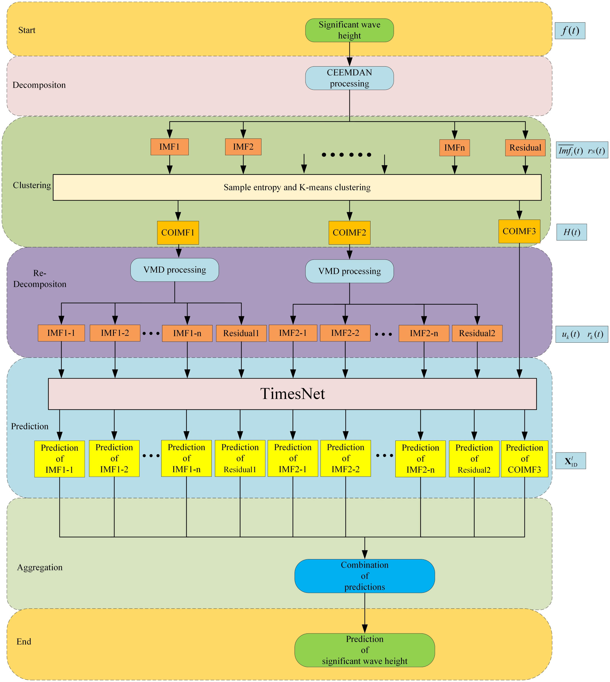
Figure 3 Flow chart of the hybrid CEEMDAN-VMD-TimesNet significant wave height prediction model.

2.8 Evaluation metrics

R², MSE, RMSE, and MAE are the four metrics used to quantify the errors between the predicted values and the actual values, which are used to evaluate the model’s performance in this research. R² is used to evaluate the degree of agreement. MSE is used to quantify the average squared difference. RMSE is used to measure the average difference. MAE is the mean of the absolute errors. The formulas are as follows:

$\begin{array}{ll}{R}^2=1-\frac{{\displaystyle {\sum }_{i=1}^n{({\widehat{y}}_i-y_i)}^2}}{{\displaystyle {\sum }_{i=1}^n{({\overline{y}}_i-y_i)}^2}}& (28)\end{array}$

$\begin{array}{ll}MSE=\frac{1}{n}{\displaystyle \sum _{i=1}^n{(y_i-{\widehat{y}}_i)}^2}& (29)\end{array}$

$\begin{array}{ll}RMSE=\sqrt{\frac{1}{n}{\displaystyle \sum _{i=1}^n{(y_i-{\widehat{y}}_i)}^2}}& (30)\end{array}$

$\begin{array}{ll}MAE=\frac{1}{n}{\displaystyle \sum _{i=1}^n\left|y_i-{\widehat{y}}_i\right|}& (31)\end{array}$

where ${\widehat{y}}_i$ represents the predicted value, y_i represents the actual value, ${\overline{y}}_i$ represents the mean of the actual values, and n represents the number of data samples.

The larger R² indicates better agreement between the predicted values and the actual values, demonstrating stronger predictive capacity of the model. In contrast, the smaller MSE, RMSE, and MAE reflect the lower error and the better predictive performance.

3 Wave datasets preprocessing

3.1 Research area

The South Sea of China was chosen for this study. The original data for significant wave height was sourced from ERA5 of the European Centre for Medium-Range Weather Forecasts (ECMWF) and covered the period from January 1, 2010, 00:00:00 UTC to December 31, 2018, 23:00:00 UTC. The time interval for significant wave height was one hour. There were a total of 78,888 valid data points. The dataset1 was selected at position 1, and the dataset2 was selected at position 2. The coordinates of position 1 were (21.50°N,113.00°E), and the coordinates of position 2 were (23.00°N,117.50°E). The location of the selected position in this paper is presented in Figure 4. The dataset1 and the dataset2 are illustrated in Figures 5, 6, respectively. The occurrence time of Typhoon Hato was from August 20, 2017, 14:00:00 UTC to August 24, 2017, 17:00:00 UTC. During the occurrence of Typhoon Hato, the maximum wind speed at position 1 is 25.08 m/s, and at position 2 is 20.84 m/s.

Figure 4

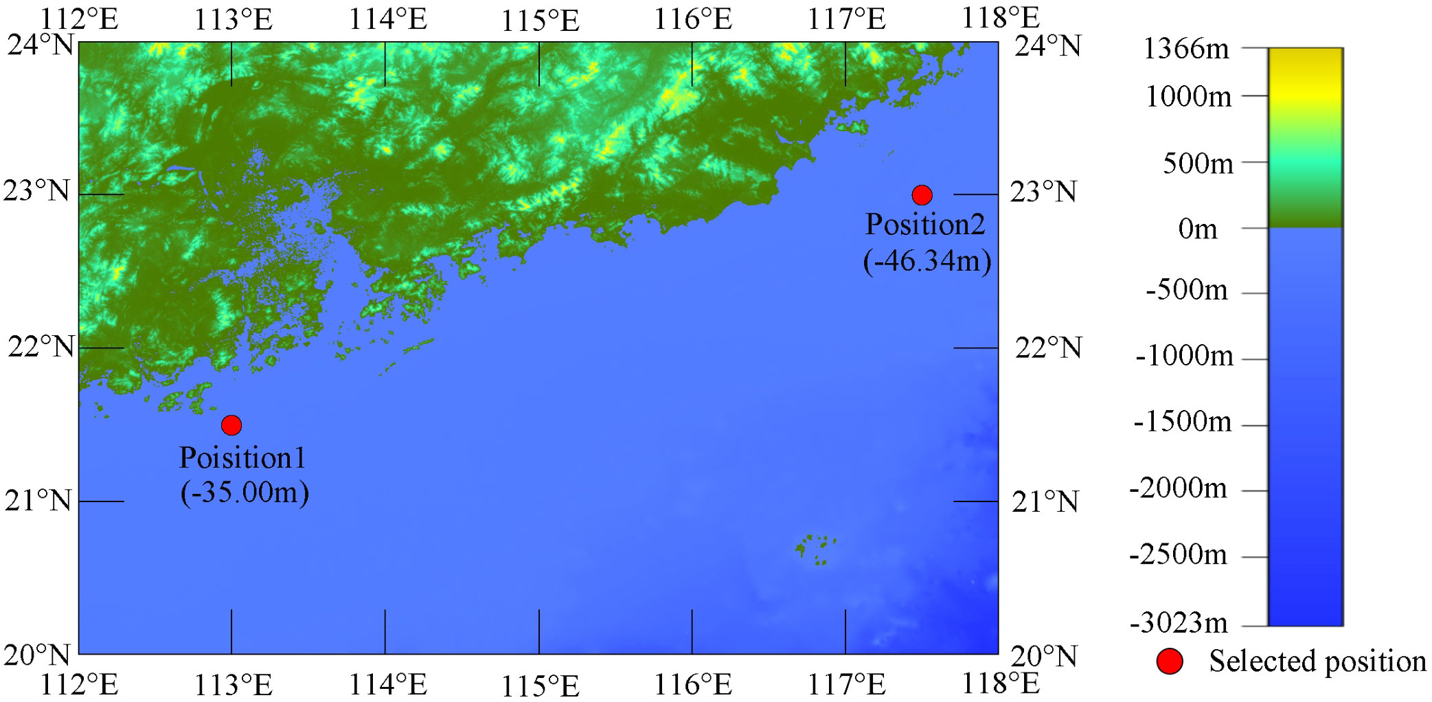
Figure 4 Distribution of the selected position in the South Sea of China.

Figure 5

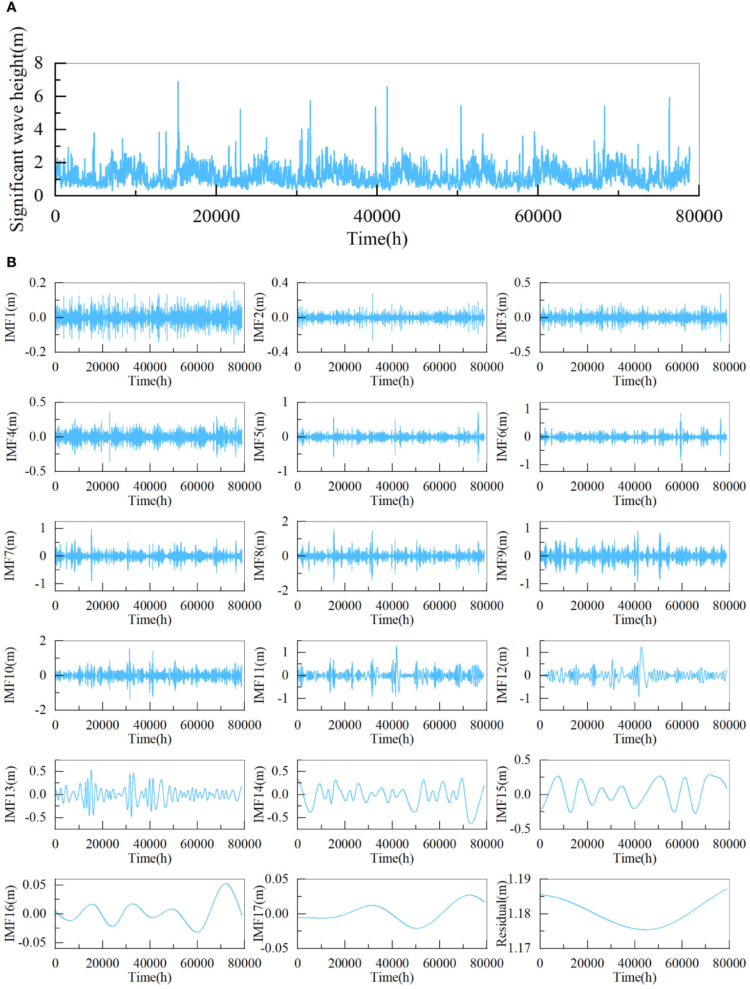
Figure 5 Significant wave height time series and decomposition results of dataset1 (A) significant wave height time series, (B) decomposition results.

Figure 6

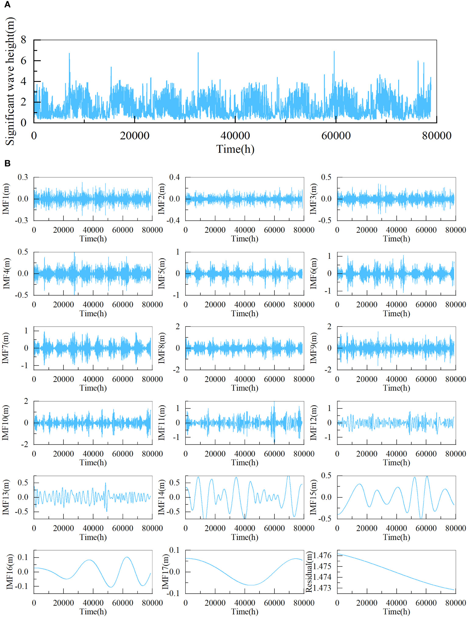
Figure 6 Significant wave height time series and decomposition results of dataset2 (A) significant wave height time series, (B) decomposition results.

3.2 Data processing

3.2.1 Siginificant wave height decomposed by CEEMDAN

This study used the pyEMD package to implement the CEEMDAN. Figures 5, 6 depict the decomposed outcomes. As shown in Figures 5, 6, the dataset1 and the dataset2 are both decomposed into 18 subsequences. It can be observed that the dataset becomes stationary through CEEMDAN decomposition.

3.2.2 Clustering decomposed sub-sequences by Sample Entropy and K-means clustering

Sample Entropy was used to measure the complexity of each IMF by the Python sample module. During the computational process, mm and r were set to 1 and 0.1, respectively. Then the Kmeans clustering algorithm was then applied to cluster subsequences into three categories. We think this classification method effectively captures the information of various component types and saves computational time. Figures 7, 8 display the calculated sample entropy values and the newly clustered IMFs, where IMF18 is the residual. As shown in Figures 7, 8, for dataset1, these IMFs can be integrated into three new COIMFs: COIMF0 (IMF1-5), COIMF1 (IMF6-8), and COIMF2 (IMF9-18). For dataset2, these IMFs can also be integrated into three new COIMFs: COIMF0 (IMF1-4), COIMF1 (IMF5-8), and COIMF2 (IMF9-18). It is clear that COIMF1 is composed of highly complex IMF components, COIMF2 is composed of moderately complex IMF components, and COIMF3 is composed of lowly complex IMF components.

Figure 7

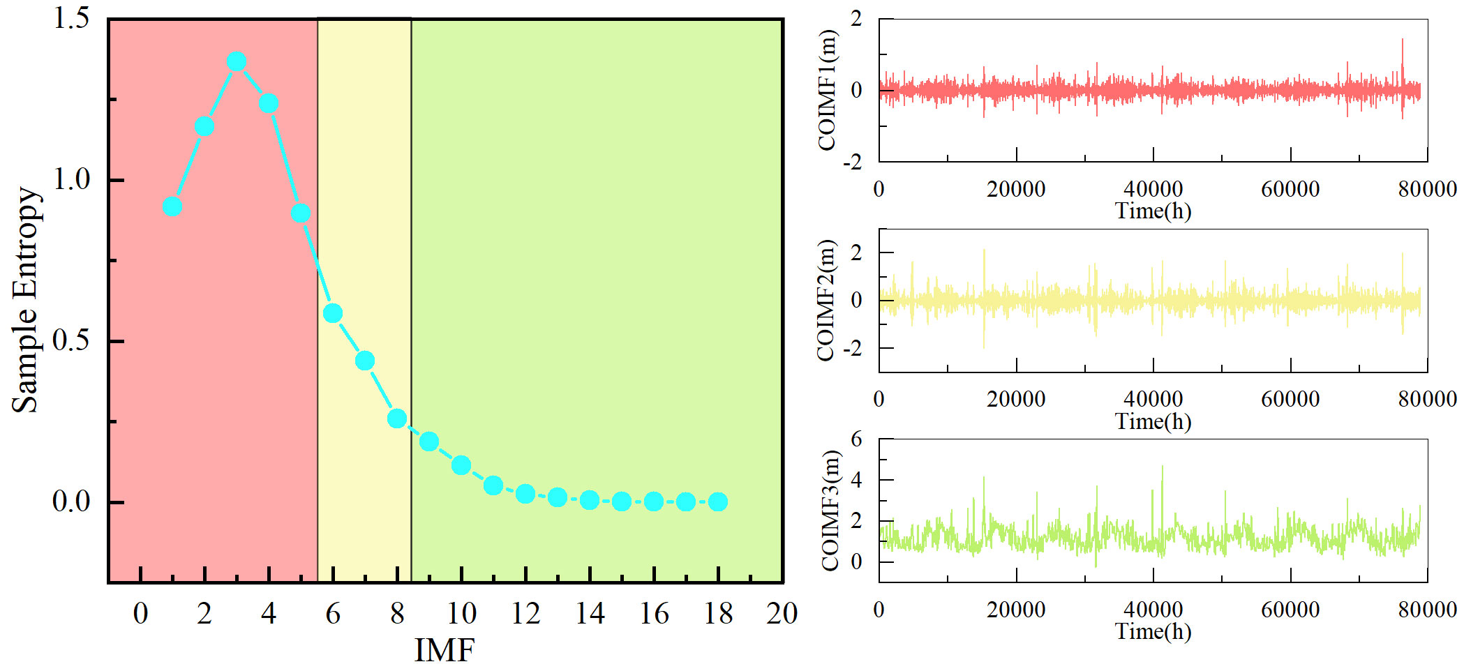
Figure 7 Sample entropy and clustering results of dataset1.

Figure 8

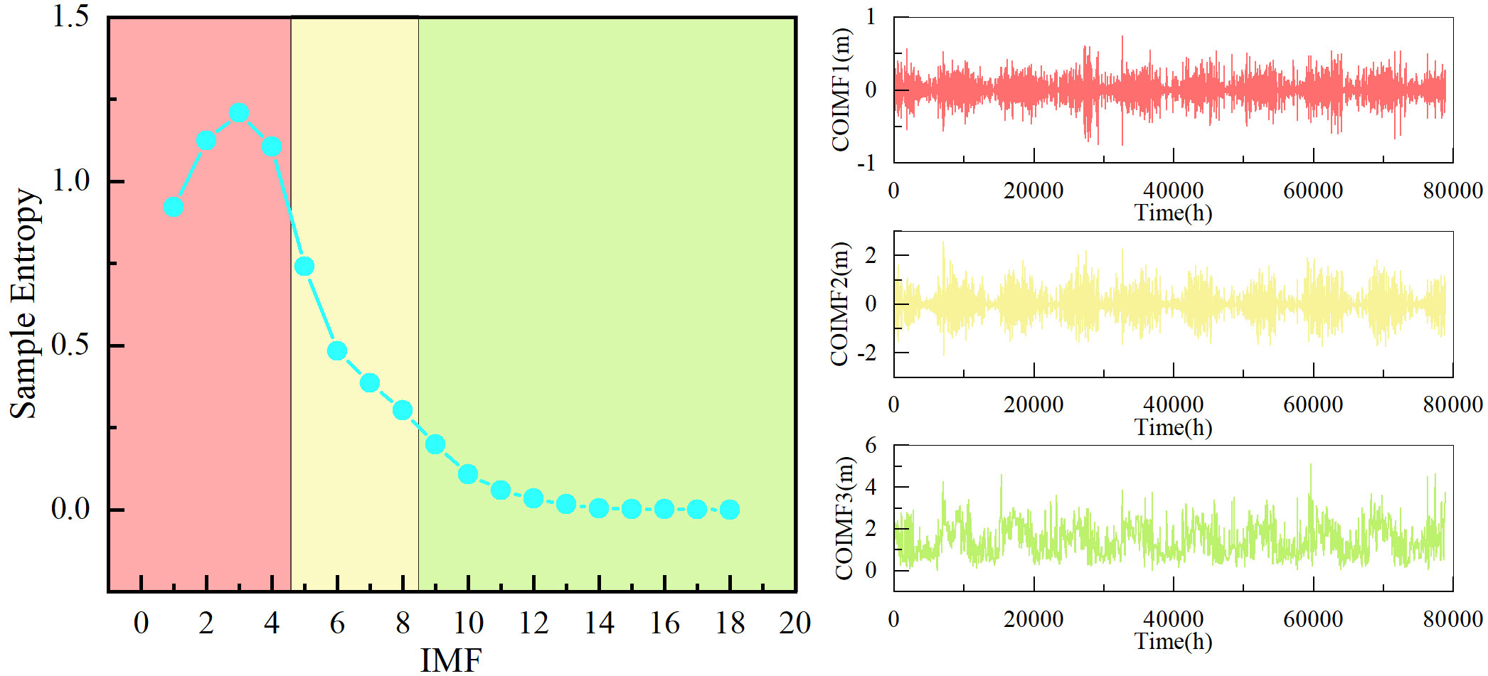
Figure 8 Sample entropy and clustering results of dataset2.

3.2.3 COIMF1 and COIMF2 decomposed by VMD

Following the first decomposition and reconstruction, the VMD was used again to decompose COIMF1 and COIMF2, aiming to enhance the stationarity and decrease the complexity of the data. Based on previous research and experience (Zhao et al., 2023), both COIMF1 and COIMF2 were decomposed into 10 IMFs and 1 residual. COIMF3 and new subsequences generated from COIMF1 and COIMF2 were subjected to maximum-minimum normalization. Then the data after normalization were predicted by TimesNet.

4 Results and discussion

4.1 Setup of model

First, the dataset partitioning should be emphasized. The dataset was partitioned into three subsets a training set including the initial 70% of the data consisting of 55221 samples, a validation set including the 10% of the data consisting of 7889 samples, and a testing set comprising the last 20% consisting of 15778 samples.

The SVM model, the GRU model, and the LSTM model are all commonly used for significant wave height prediction and are regularly employed in various studies for conducting comparative analyses (Meng et al., 2021; Song et al., 2022). Thus, in this research, we selected these models to assess the performance of our proposed model.

The experiment was conducted in a Python 3.7 environment. Based on previous research and experimental results (Meng et al., 2021), the kernel of the SVM model was Radial Basis Function(RBF). The tol, C and gamma of the SVM model were 0.001, 1 and 0.1, respectively. The remaining parameters were set by default in the scikit-learn.

Based on previous experience and multiple experiments, the GRU model and the LSTM model were both divided into three layers input layer, hidden layer, and output layer. The hidden layer consisted of 32 neurons. The MSE was chosen as the loss function, and the Adam optimizer was used. Dropout was set to 0.2. The batch size was set to 32, and the number of epochs was set to 100. To prevent overfitting, early stopping was implemented with a patience of 10. The timestep was set to 7, meaning that the significant wave height of the current hour was considered to be related to the previous seven hours.

For the TimesNet model, the sequence length and label length were both set to 12 based on previous experience and multiple experiments. The loss function remained as MSE, and the optimizer was still Adam. The batch size and number of epochs were set to 32 and 7, respectively. Dropout was set to 0.2. To prevent overfitting, early stopping was implemented with a patience of 3. The number of heads was set to 8, the dimension of models was set to 16, and the attention factor was set to 5.

In order to facilitate the analysis, this study selected 400 data points to create comparative figures.

The time span covered was from August 18, 2017, 00:00:00 UTC to September 3, 2017, 15:00:00 UTC. It is worth noting that Typhoon Hato occurred during this time period.

4.2 Multi-step prediction results by different models

To evaluate the accuracy of the predictions, Tables 1, 2 record the error statistics of the results of the dataset by each model. Tables 3, 4 record the error statistics of the results of COIMF1, COIMF2 and COIMF3 by different models. Figures 9, 10 present the comparison between the predicted and actual values for both models. “1h” in Figures 9, 10 represents August 18, 2017, at 00:00:00 UTC. The occurrence time of Typhoon Hato in Figures 9, 10 is from 63h to 162h, which is between the dotted lines. Figure 11 shows comparison of RMSE during the typhoon period in different prediction lead time.

Table 1

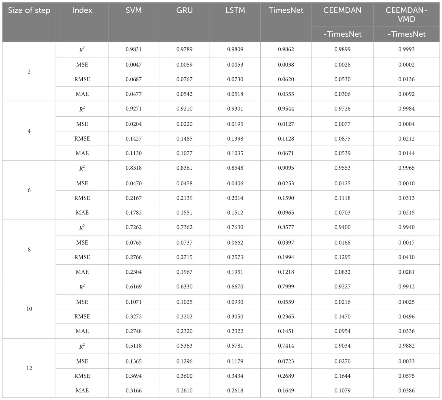
Table 1 Error measures of multi-step predictions of dataset1 by different models.

Table 2

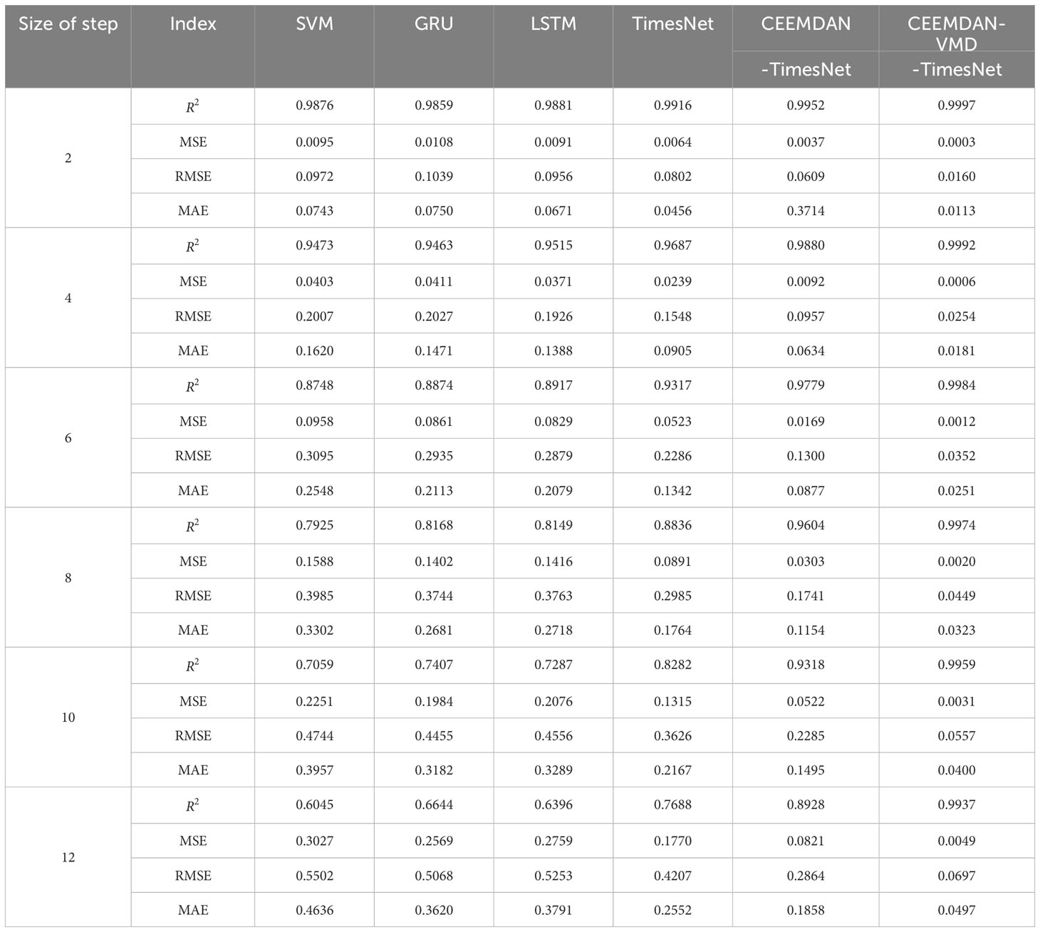
Table 2 Error measures of multi-step predictions of dataset2 by different models.

Table 3

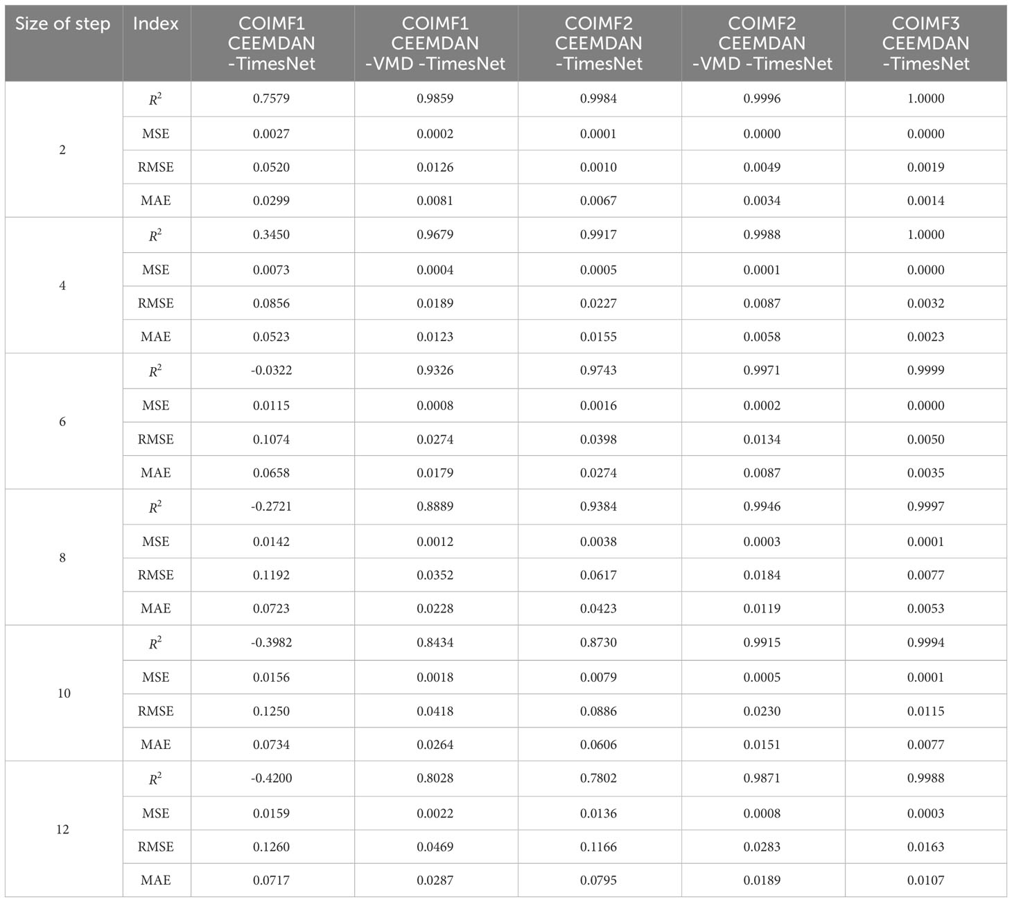
Table 3 Error measures of multi-step predictions of COIMFs for dataset1 by different models.

Table 4

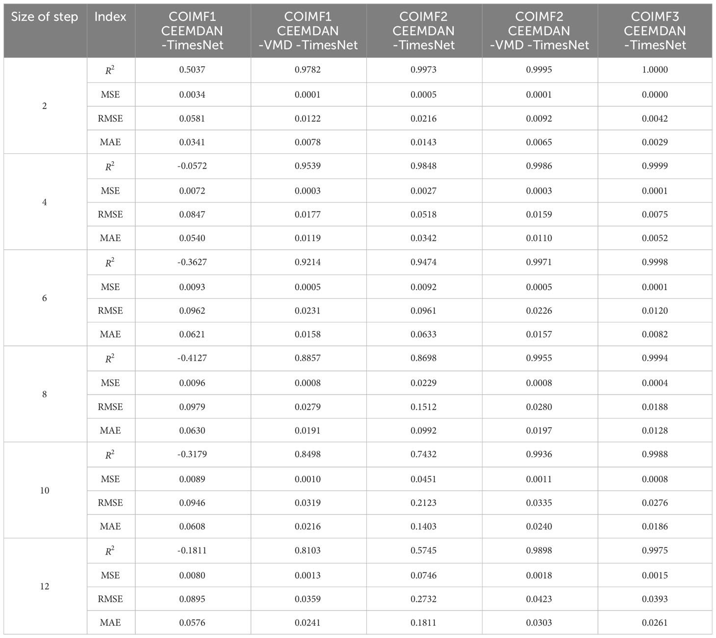
Table 4 Error measures of multi-step predictions of COIMFs for dataset2 by different models.

Figure 9

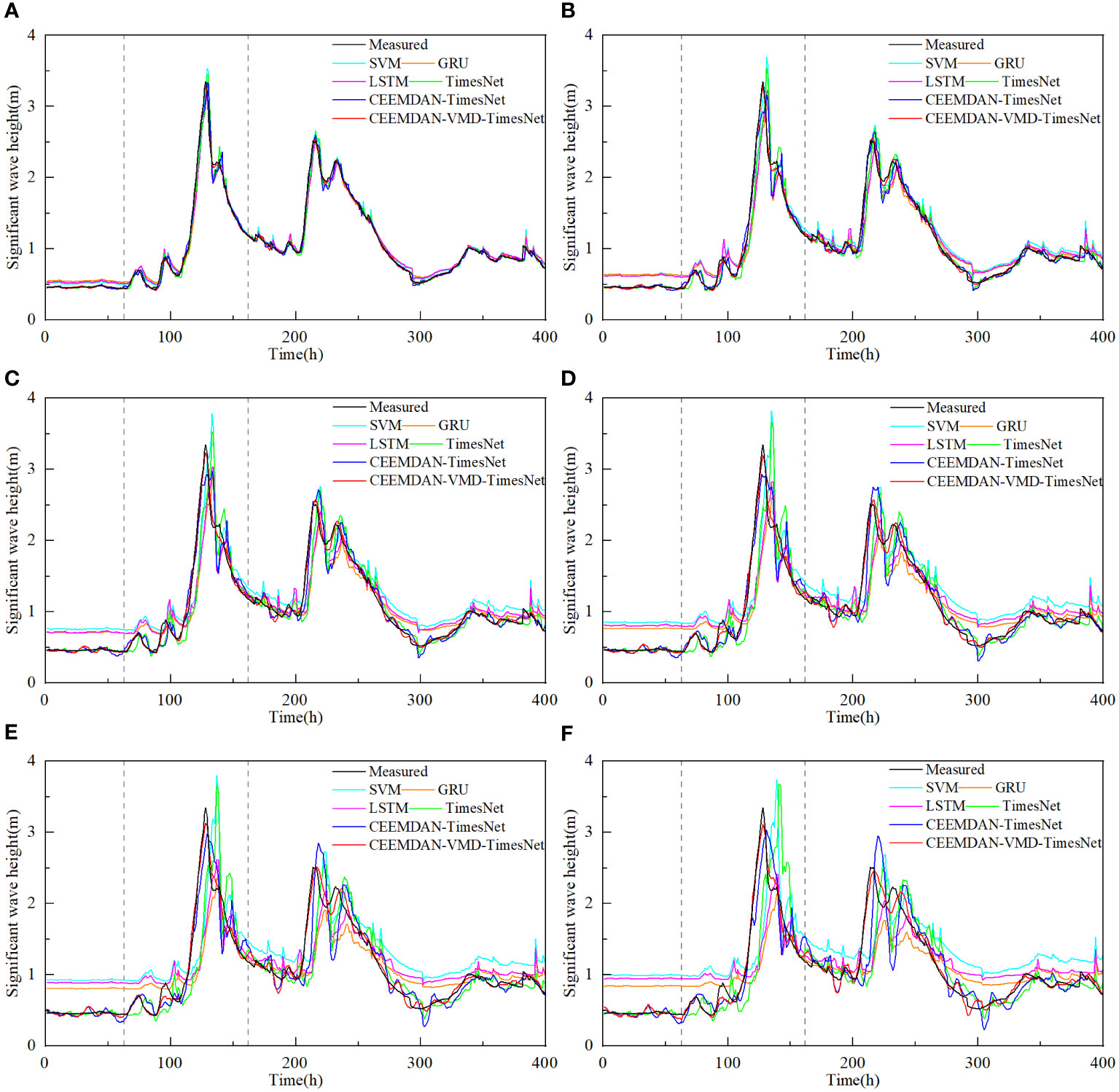
Figure 9 Predictions of significant wave height of dataset1 by different models for several future hours (A) 2 hours, (B) 4 hours, (C) 6 hours, (D) 8 hours, (E) 10 hours and (F) 12 hours.

Figure 10

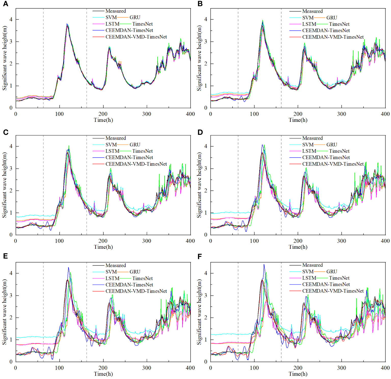
Figure 10 Predictions of significant wave height of dataset2 by different models for several future hours (A) 2 hours, (B) 4 hours, (C) 6 hours, (D) 8 hours, (E) 10 hours and (F) 12 hours.

Figure 11

Figure 11 Comparison of RMSE during the typhoon period in different prediction lead time for dataset1 and dataset2 (A) dataset1, (B) dataset2.

4.3 Discussion of the prediction results

From Tables 1, 2, it can be observed that all models have shown good performance when the number of prediction steps is small, and the accuracy of the prediction results by the TimesNet model is higher compared to that of other models. Furthermore, as the number of steps increases, the difference becomes more pronounced. For dataset1, when the number of prediction steps becomes twelve, R² of prediction results by the SVM model, the GRU model and the LSTM model are only 0.5118, 0.5363 and 0.5781, respectively. While R² of prediction results by the TimesNet model can reach 0.7414. This phenomenon occurs because the SVM model, the GRU model and the LSTM model all need to calculate the value of the current time before using it to predict the next value. This process introduces cumulative errors, which accumulate and become larger as the number of steps increases. On the other hand, the TimesNet model avoids cumulative errors by connecting each point in the time series with other points. Additionally, the TimesNet model can effectively capture intraperiod- and interperiod-variations, resulting in a minimal decrease in the accuracy of the predictions with an increasing number of steps. Wu et al. (2022) conducted research on both short-term and long-term forecasting for time series data and found that the TimesNet model outperformed the LSTM model in terms of prediction accuracy, which aligns with the findings of this study. Considering the advantages of the TimesNet model, this study chooses to conduct further research using the TimesNet model.

Observing Tables 1, 2, it is found that there has been a substantial improvement in the accuracy of the predictions after decomposing the original significant wave height with CEEMDAN and clustering IMFs. The decrease in accuracy of the CEEMDAN-TimesNet model is lower compared to the TimesNet model. For the 12-step ahead prediction results of dataset1, R² of the prediction results by the CEEMDAN-TimesNet model is improved by 21.85% compared to the prediction results by the TimesNet model. MSE, RMSE and MAE are decreased by 62.66%, 38.86% and 34.57%, respectively. For the 12-step ahead prediction results of dataset2, R² of the prediction results by the CEEMDAN-TimesNet model is improved by 16.13% compared to the prediction results by the TimesNet model. MSE, RMSE and MAE are decreased by 53.62%, 31.92% and 27.19%, respectively. The wave time series has non-stationary properties (Londhe and Panchang, 2006), which affects the prediction accuracy. Applying CEEMDAN and clustering improves prediction accuracy by reducing the non-stationarity of the original significant wave height.

A more detailed analysis is required for the prediction results of COIMFs for further enhancements to the CEEMDAN-TimesNet model. From Tables 3, 4, it is evident that the main source of error is COIMF1 and COIMF2. The prediction results of COIMF1 are not satisfactory even for the small step-ahead prediction. As the prediction duration increases, the accuracy becomes worse. R² of the prediction results is even negative, which is unacceptable. COIMF2 performs better than COIMF1 in terms of prediction accuracy when the prediction steps are small. However, as the prediction steps increase, the prediction accuracy of COIMF2 also decreases noticeably. Surprisingly, COIMF3 maintains a relatively stable level, showing consistently outstanding performance in prediction. The reason for this phenomenon is that COIMF1 is formed by combining IMFs with high sample entropy, resulting in the highest complexity and non-stationarity, which introduces significant errors in the prediction results. COIMF3, on the other hand, is composed of IMF components with low complexity, making it stationary and highly accurate in prediction. COIMF2 consists of IMFs with moderate complexity. Therefore, COIMF2 falls between COIMF1 and COIMF3 in terms of prediction accuracy.

Given the poor prediction results of COIMF1 and COIMF2, COIMF1 and COIMF2 are decomposed by VMD again, while COIMF3 remains unchanged. From Tables 3, 4, it can be observed that prediction results of COIMF1 and COIMF2 exhibit a significant improvement after decomposition, regardless of the number of prediction steps. The enhancement in the prediction of COIMF1 and COIMF2 has resulted in an overall improvement in prediction results of significant wave height. For the 12-step ahead prediction results of dataset1, R² of the prediction results by the CEEMDAN-VMD-TimesNet model is improved by 33.29% compared to the prediction results by the TimesNet model. MSE, RMSE and MAE are decreased by 95.44%, 78.62% and 76.59%, respectively. For the 12-step ahead prediction results of dataset2, R² of the prediction results by the CEEMDAN-VMD-TimesNet model is improved by 29.25% compared to the prediction results by the TimesNet model. MSE, RMSE and MAE are decreased by 97.23%, 83.43% and 80.53%, respectively. The accuracy of the CEEMDAN-VMD-TimesNet model far surpasses all the models mentioned earlier. The analysis leads to the conclusion that the CEEMDAN-VMD-TimesNet model has a clear advantage in prediction, especially when predicting multiple steps, significantly improving the prediction results.

Figures 9, 10 illustrate the performance of all models in predicting typhoons. When the number of prediction steps is small, all models perform well by capturing the overall characteristics of the original significant wave height and accurately predicting wave peaks and troughs without massive phase shifts. However, as the prediction duration increases, the SVM model, the GRU model, the LSTM model and the TimesNet model show noticeable phase shifts in the predictions of wave peaks and troughs due to the effects of non-stationarity. On the other hand, the CEEMDAN-TimesNet model provides more accurate predictions compared to these models, greatly alleviating the occurrence of phase shifts. The CEEMDAN-VMD-TimesNet model stands out among all the models. The twelve-step-ahead prediction results by the CEEMDAN-VMD-TimesNet model remain highly consistent with the original significant wave height in terms of both trend and extreme values, with minimal phase shifts. Figure 11 shows the comparison of RMSE during the typhoon period in different prediction lead time between the CEEMDAN-VMD-TimesNet model and other models. Regardless of the prediction lead time, the CEEMDAN-VMD-TimesNet model consistently maintains the lowest RMSE. As the prediction lead time increases, RMSE grows at the slowest rate. When the prediction lead time is twelve, RMSE is much lower than other models, resulting in quite satisfactory accuracy. Thus, it can be inferred that the application of the CEEMDAN-VMD-TimesNet model for typhoon prediction is feasible.

5 Conclusion

Wave energy is a significant and environmentally friendly source of energy that has a wide range of applications. Accurate prediction of significant wave height plays a crucial role in wave energy generation. However, due to the complexity of significant wave height data, accurate prediction of significant wave height remains a challenge. In this study, a hybrid model called CEEMADN-VMD-TimesNet was proposed for predicting significant wave height. The significant wave height used was sourced from ERA5 of the European Centre for Medium-Range Weather Forecasts (ECMWF), and two positions in the South Sea of China were selected. The SVM model, the GRU model, the LSTM model, the TimesNet model, the CEEMADN-TimesNet model and the CEEMDAN-VMD-TimesNet model were built to predict significant wave height. By comparing the performance of these models, the following findings were obtained:

The SVM model, the GRU model and the LSTM model exhibit high accuracy for the small step-ahead prediction, but as the prediction steps increase, the prediction accuracy rapidly declines. Regardless of the number of prediction steps, the TimesNet model outperforms the SVM model, the GRU model and the LSTM model in terms of prediction accuracy, and this advantage becomes more pronounced for the large step-ahead prediction.

The non-stationarity of the original significant wave height is reduced by decomposing the original significant wave height with CEEMDAN and clustering IMFs. The CEEMADN-TimesNet model demonstrates superior accuracy in terms of prediction compared to the TimesNet model.

Components with high and moderate complexity are the main source of prediction errors. The accuracy of prediction results of significant wave height can be greatly improved by decomposing the components with high and moderate complexity using VMD. The CEEMADN-VMD-TimesNet model has the strongest prediction capability among the models used in this study.

The CEEMADN-VMD-TimesNet model can accurately predict trends and extreme values of significant wave height with minimal phase shifts during the Typhoon Hato period even for the large step-ahead prediction.

Although the proposed hybrid model achieves good accuracy, it still leaves questions for us to ponder. We did not compare the computation time of the secondary decomposition model with other models. The effect of the secondary decomposition on the computation time needs to be further investigated. Besides, we did not compare the results of the CEEMADN-VMD-TimesNet model with the NWP model, which is a limitation of our study. In future, this will be the focus of our research.

Data availability statement

The raw data supporting the conclusions of this article will be made available by the authors, without undue reservation.

Author contributions

TD: Conceptualization, Methodology, Software, Writing – original draft. DW: Data curation, Funding acquisition, Supervision, Writing – review & editing. YL: Data curation, Software, Validation, Writing – review & editing. LS: Data curation, Software, Supervision, Writing – review & editing. XZ: Software, Validation, Writing – review & editing, Investigation.

Funding

The author(s) declare that financial support was received for the research, authorship, and/or publication of this article. The present work is sponsored by the National Natural Science Foundation of China (Grant No.42176166; No.41776024) and Major Project of Power Construction Corporation of China, Ltd (DJ-ZDXM-2022-28; KJXMWW-2023-01).

Acknowledgments

The significant wave height used was sourced from ERA5 of the European Centre for Medium-Range Weather Forecasts (ECMWF). We would like to acknowledge the ECMWF.

Conflict of interest

Authors YL and LS were employed by the company Municipal Engineering Corporation Limited. Author XZ was employed by the company Power China Kunming Engineering Corporation Limited.

The remaining authors declare that the research was conducted in the absence of any commercial or financial relationships that could be construed as a potential conflict of interest.

Publisher’s note

All claims expressed in this article are solely those of the authors and do not necessarily represent those of their affiliated organizations, or those of the publisher, the editors and the reviewers. Any product that may be evaluated in this article, or claim that may be made by its manufacturer, is not guaranteed or endorsed by the publisher.

References

Agrawal J., Deo M. (2002). On-line wave prediction. Mar. struct. 15, 57–74. doi: 10.1016/S0951-8339(01)00014-4

CrossRef Full Text | Google Scholar

Ali M., Prasad R. (2019). Significant wave height forecasting via an extreme learning machine model integrated with improved complete ensemble empirical mode decomposition. Renewableand Sustain. Energy Rev. 104, 281–295. doi: 10.1016/j.rser.2019.01.014

CrossRef Full Text | Google Scholar

Amunugama M., Suzuyama K., Manawasekara C., Tanaka Y., Xia Y. (2020). Typhoon-induced storm surge analysis with coast on different modelled forcing. J. Japan Soc. Civil Eng. Ser. B3 (Ocean Engineering) 76, I_210–I_215. doi: 10.2208/jscejoe.76.2_I_210

CrossRef Full Text | Google Scholar

Bertsekas D. P. (1976). Multiplier methods A survey. Automatica 12, 133–145. doi: 10.1016/S1474-6670(17)67759-0

CrossRef Full Text | Google Scholar

Bethel B. J., Sun W., Dong C., Wang D. (2022). Forecasting hurricane-forced significant wave heights using a long short-term memory network in the Caribbean sea. Ocean Sci. 18, 419–436. doi: 10.5194/os-18-419-2022

CrossRef Full Text | Google Scholar

Chang H.-K., Liou J.-C., Liu S.-J., Liaw S.-R. (2011). Simulated wave-driven ANN model for typhoon waves. Adv. Eng. Softw. 42, 25–34. doi: 10.1016/j.advengsoft.2010.10.014

CrossRef Full Text | Google Scholar

Chen T., Zhang Q., Wu Y., Ji C., Yang J., Liu G. (2018). Development of a wave-current model through coupling of fvcom and swan. Ocean Eng. 164, 443–454. doi: 10.1016/j.oceaneng.2018.06.062

CrossRef Full Text | Google Scholar

Deo M. C., Jha A., Chaphekar A., Ravikant K. (2001). Neural networks for wave forecasting. Ocean Eng. 28, 889–898. doi: 10.1016/S0029-8018(00)00027-5

CrossRef Full Text | Google Scholar

Dragomiretskiy K., Zosso D. (2013). Variational mode decomposition. IEEE Trans. Signal Process. 62, 531–544. doi: 10.1109/TSP.2013.2288675

CrossRef Full Text | Google Scholar

Duan W. Y., Huang L. M., Han Y., Huang D. T. (2016). A hybrid emd-ar model for nonlinear and non-stationary wave forecasting. J. Zhejiang University-SCIENCE A 17, 115–129. doi: 10.1631/jzus.A1500164

CrossRef Full Text | Google Scholar

Fan S., Xiao N., Dong S. (2020). A novel model to predict significant wave height based on long short-term memory network. Ocean Eng. 205, 107298. doi: 10.1016/j.oceaneng.2020.107298

CrossRef Full Text | Google Scholar

Hao W., Sun X., Wang C., Chen H., Huang L. (2022). A hybrid emd-lstm model for non-stationary wave prediction in offshore China. Ocean Eng. 246, 110566. doi: 10.1016/j.oceaneng.2022.110566

CrossRef Full Text | Google Scholar

He K., Zhang X., Ren S., Sun J. (2016). “Deep residual learning for image recognition,” in Proceedings of the IEEE conference on computer vision and pattern recognition. (Las Vegas, NV, USA: IEEE) 770–778. doi: 10.1109/CVPR.2016.90

CrossRef Full Text | Google Scholar

Hestenes M. R. (1969). Multiplier and gradient methods. J. optim. Theory Appl. 4, 303–320. doi: 10.1007/BF00927673

CrossRef Full Text | Google Scholar

Hochreiter S., Schmidhuber J. (1997). Long short-term memory. Neural Comput. 9, 1735–1780. doi: 10.1162/neco.1997.9.8.1735

PubMed Abstract | CrossRef Full Text | Google Scholar

Huang N. E., Shen Z., Long S. R., Wu M. C., Shih H. H., Zheng Q., et al. (1998). The empirical mode decomposition and the hilbert spectrum for nonlinear and non-stationary time series analysis. Proc. R. Soc. London. Ser. A mathematic. Phys. Eng. Sci. 454, 903–995. doi: 10.1098/rspa.1998.0193

CrossRef Full Text | Google Scholar

Li X., Cao J., Guo J., Liu C., Wang W., Jia Z., et al. (2022). Multi-step forecasting of ocean wave height using gate recurrent unit networks with multivariate time series. Ocean Eng. 248, 110689. doi: 10.1016/j.oceaneng.2022.110689

CrossRef Full Text | Google Scholar

Londhe S., Panchang V. (2006). One-day wave forecasts based on artificial neural networks. J. Atmos. ocean. Technol. 23, 1593–1603. doi: 10.1175/JTECH1932.1

CrossRef Full Text | Google Scholar

Mahjoobi J., Mosabbeb E. A. (2009). Prediction of significant wave height using regressive support vector machines. Ocean Eng. 36, 339–347. doi: 10.1016/j.oceaneng.2009.01.001

CrossRef Full Text | Google Scholar

Meng F., Song T., Xu D., Xie P., Li Y. (2021). Forecasting tropical cyclones wave height using bidirectional gated recurrent unit. Ocean Eng. 234, 108795. doi: 10.1016/j.oceaneng.2021.108795

CrossRef Full Text | Google Scholar

Meng F., Xu D., Song T. (2022). Atdnns: An adaptive time–frequency decomposition neural network-based system for tropical cyclone wave height real-time forecasting. Future Gen. Comput. Syst. 133, 297–306. doi: 10.1016/j.future.2022.03.029

CrossRef Full Text | Google Scholar

Reikard G., Robertson B., Bidlot J.-R. (2015). Combining wave energy with wind and solar: Short-term forecasting. Renewable Energy 81, 442–456. doi: 10.1016/j.renene.2015.03.032

CrossRef Full Text | Google Scholar

Reikard G., Robertson B., Bidlot J.-R. (2017). Wave energy worldwide Simulating wave farms, forecasting, and calculating reserves. Int. J. Mar. Energy 17, 156–185. doi: 10.1016/j.ijome.2017.01.004

CrossRef Full Text | Google Scholar

Reikard G., Rogers W. E. (2011). Forecasting ocean waves Comparing a physics-based model with statistical models. Coast. Eng. 58, 409–416. doi: 10.1016/j.coastaleng.2010.12.001

CrossRef Full Text | Google Scholar

Richman J. S., Moorman J. R. (2000). Physiological time-series analysis using approximate entropy and sample entropy. Am. J. physiology-heart Circulatory Physiol. 278, H2039–H2049. doi: 10.1152/ajpheart.2000.278.6.H2039

CrossRef Full Text | Google Scholar

Sharma T., Bedi J., Anand A., Aggarwal A. (2023). Wave height prediction in maritime transportation using decomposition based learning. IEEE Trans. Intell. Transport. Syst. 1–10. doi: 10.1109/TITS.2023.3322192

CrossRef Full Text | Google Scholar

Soares C. G., Cunha C. (2000). Bivariate autoregressive models for the time series of significant wave height and mean period. Coast. Eng. 40, 297–311. doi: 10.1016/S0378-3839(00)00015-6

CrossRef Full Text | Google Scholar

Song T., Han R., Meng F., Wang J., Wei W., Peng S. (2022). A significant wave height prediction method based on deep learning combining the correlation between wind and wind waves. Front. Mar. Sci. 9. doi: 10.3389/fmars.2022.983007

PubMed Abstract | CrossRef Full Text | Google Scholar

Song T., Wang J., Huo J., Wei W., Han R., Xu D., et al. (2023). Prediction of significant wave height based on eemd and deep learning. Front. Mar. Sci. 10. doi: 10.3389/fmars.2023.1089357

CrossRef Full Text | Google Scholar

Torres M. E., Colominas M. A., Schlotthauer G., Flandrin P. (2011). “A complete ensemble empirical mode decomposition with adaptive noise,” in 2011 IEEE international conference on acoustics, speech and signal processing (ICASSP). (Prague, Czech Republic: IEEE) 4144–4147. doi: 10.1109/ICASSP.2011.5947265

CrossRef Full Text | Google Scholar

Vaswani A., Shazeer N., Parmar N., Uszkoreit J., Jones L., Gomez A. N., et al. (2017). “Attention is all you need,” in Advances in neural information processing systems. (Long Beach, california, USA: Neural Information Processing Systems Foundation, Inc. (NeurlPS)), 30. doi: 10.48550/arXiv.1706.03762

CrossRef Full Text | Google Scholar

Vijayan L., Huang W., Ma M., Ozguven E., Ghorbanzadeh M., Yang J., et al. (2023). Improving the accuracy of hurricane wave modeling in Gulf of Mexico with dynamically-coupled swan and adcirc. Ocean Eng. 274, 114044. doi: 10.1016/j.oceaneng.2023.114044

CrossRef Full Text | Google Scholar

Wang W., Tang R., Li C., Liu P., Luo L. (2018). A bp neural network model optimized by mind evolutionary algorithm for predicting the ocean wave heights. Ocean Eng. 162, 98–107. doi: 10.1016/j.oceaneng.2018.04.039

CrossRef Full Text | Google Scholar

Wu H., Hu T., Liu Y., Zhou H., Wang J., Long M. (2022). Timesnet: Temporal 2d-variation modeling for general time series analysis. arXiv preprint arXiv. doi: 10.48550/arXiv.2210.02186

CrossRef Full Text | Google Scholar

Wu Z., Huang N. E. (2009). Ensemble empirical mode decomposition: a noise-assisted data analysis method. Adv. adapt. Data Anal. 1, 1–41. doi: 10.1142/S1793536909000047

CrossRef Full Text | Google Scholar

Wu H., Xu J., Wang J., Long M. (2021). Autoformer: Decomposition transformers with auto-correlation for long-term series forecasting. Adv. Neural Inf. Process. Syst. 34, 22419–22430. doi: 10.48550/arXiv.2106.13008

CrossRef Full Text | Google Scholar

Yang Z., Huang W. (2022). Wave height estimation from x-band radar data using variational mode decomposition. IEEE Geosci. Remote Sens. Lett. 19, 1–5. doi: 10.1109/LGRS.2022.3195675

CrossRef Full Text | Google Scholar

Zhao L., Li Z., Qu L., Zhang J., Teng B. (2023). A hybrid vmd-lstm/gru model to predict non-stationary and irregular waves on the east coast of China. Ocean Eng. 276, 114136. doi: 10.1016/j.oceaneng.2023.114136

CrossRef Full Text | Google Scholar

Zhou H., Zhang S., Peng J., Zhang S., Li J., Xiong H., et al. (2021). “Informer Beyond efficient transformer for long sequence time-series forecasting,” in Proceedings of the AAAI conference on artificial intelligence. (Palo Alto, California USA: AAAI), Vol. 35. 11106–11115. doi: 10.1609/aaai.v35i12.17325

CrossRef Full Text | Google Scholar